
the Creative Commons Attribution 4.0 License.
the Creative Commons Attribution 4.0 License.
 | 14 Jul 2026
Opposing entrainment effects of cloud droplet sedimentation during the pre-breakup stage of the stratocumulus to cumulus transition
Moritz Schnelke
Maike Ahlgrimm
Anna Possner
Cloud droplet sedimentation is known to influence the evolution of the stratocumulus-topped boundary layer by reducing entrainment. Although this mechanism is well studied regarding the early evolution of stratocumuli, its sustained effects over longer time scales remain largely unexplored. Here, we use large-eddy simulations to investigate how sedimentation influences stratocumulus development in the context of the stratocumulus to cumulus transition. We conduct 48 h long simulations of 10 transects in the Northeast Pacific, covering the full deepening stage before cloud breakup. All sedimentation cases show the previously reported initial reduction in entrainment, whereas the later stages reveal different effects depending on the cloud's liquid water path (LWP). While the more frequent precipitating, high-LWP (LWP ) cases continue to exhibit weaker entrainment, the non-precipitating, low-LWP (LWP ) cases reverse the initial effect and show stronger entrainment. In those radiatively unsaturated low-LWP clouds, the increase in LWP due to the initial entrainment reduction initiates a feedback chain that amplifies LWP, longwave cooling, and turbulent circulations in the boundary layer, ultimately leading to increased entrainment. Initial studies showed that droplet sedimentation reduces entrainment in short (≤6 h) simulations of low-LWP clouds, which has been extrapolated in the literature to all stratocumuli on much longer time scales. Our results suggest that this extrapolation is indeed correct in common high-LWP clouds, although it had previously been inferred from the rare low-LWP regime, where the opposite is found. Meanwhile, we find that cloud breakup remains largely unaffected across the transition.
- Article
(8805 KB) - Full-text XML
- BibTeX
- EndNote


Stratocumulus clouds are an important contributor to Earth's cooling, as they reflect a high amount of incoming shortwave radiation and have only little effect on outgoing longwave radiation (Wood, 2012). The marine type occurs frequently over the midlatitude oceans as well as the eastern basins of subtropical oceans (Klein and Hartmann, 1993; Wood, 2012). Subtropical stratocumulus clouds often organise in vast semi-permanent decks near the coasts, which gradually break up as they are advected over warmer waters in the direction of the free ocean (Klein and Hartmann, 1993; Sandu et al., 2010). This phenomenon is known as the stratocumulus to cumulus transition (SCT). The SCT has been studied extensively in the past decades using observations (e.g. Zhou et al., 2015; Eastman and Wood, 2016; Wood et al., 2018; Bretherton et al., 2019; Mohrmann et al., 2019; Sarkar et al., 2019; Christensen et al., 2020) as well as numerical simulations (e.g. Krueger et al., 1995; Bretherton and Wyant, 1997; Wyant et al., 1997; Sandu et al., 2010; Sandu and Stevens, 2011; van der Dussen et al., 2013; de Roode et al., 2016; Yamaguchi et al., 2017; Blossey et al., 2021; Erfani et al., 2022; Kurowski et al., 2025). The main dynamical driver is the rising sea surface temperature (SST) that promotes decoupling of the stratocumulus deck from the surface. Cumulus clouds start to form in a mixed layer below cloud-base and subsequently penetrate into the above-lying deck. Increased entrainment together with overshooting cumuli eventually leads to the dissipation of the stratocumulus deck and its replacement by shallow cumuli (Bretherton and Wyant, 1997; Wyant et al., 1997). It has further been demonstrated recently that the diurnal cycle is profoundly impacting the SCT, as the coupling of the boundary layer to the moisture supply differs between day-time and night-time conditions. While the stratocumulus deck is mostly coupled to the moisture supply at night, either directly or through the mixed layer cumuli, solar insolation drives decoupling throughout the day (van der Dussen et al., 2013; Kurowski et al., 2025).
While the dynamical mechanism is widely accepted, it has been shown in recent years that the SCT is also influenced by microphysically induced processes like precipitation. Numerical studies utilising large-eddy simulations (LES) are largely in agreement that precipitation can have an accelerating impact on the SCT (Sandu and Stevens, 2011; Yamaguchi et al., 2017; Blossey et al., 2021; Erfani et al., 2022). In Yamaguchi et al. (2017), the authors even found a precipitation-driven transition through drizzle formation in the sub-cloud layer cumuli, that cleanses the stratocumuli from aerosols in a positive feedback loop. In contrast, most observational studies remain inconclusive about the effect of precipitation due to the challenge of disentangling individual mechanisms (Zhou et al., 2015; Eastman and Wood, 2016; Mohrmann et al., 2019; Sarkar et al., 2019).
One mechanism impacting two key drivers of the SCT, precipitation and cloud-top entrainment (hereafter entrainment), is cloud droplet sedimentation. This process has been neglected until Ackerman et al. (2004) reported on the reduction of the entrainment velocity in stratocumulus clouds in LES, when including droplet sedimentation. This was confirmed and further quantified by Bretherton et al. (2007), Wyant et al. (2007), Ackerman et al. (2009), and Hill et al. (2009). The main reason is that the removal of cloud droplets from the entrainment zone reduces the evaporation rate, which in turn slows down the entrainment rate. More recently, the analysis was extended using direct numerical simulations (DNS) by de Lozar and Mellado (2017), Schulz and Mellado (2019), and Pistor and Mellado (2025). The study of de Lozar and Mellado (2017) revealed that additionally to the reduction of evaporation, a positive buoyancy flux is introduced through the sedimenting droplets, further reducing entrainment. Moreover, cloud droplet sedimentation acts on precipitation development, as shown by Wyant et al. (2007), Savic-Jovcic and Stevens (2008), and Ackerman et al. (2009). They found that precipitation rates are reinforced at cloud-base as well as the surface in the presence of cloud droplet sedimentation, leading to an overall counteracting effect regarding the stratocumulus to cumulus transition: While droplet sedimentation reduces entrainment, impeding the SCT, it also enhances precipitation, that can cause an acceleration of the SCT.
Although there have been individual investigations with regards to both effects, to our knowledge, none of the previous studies considered the impact of cloud droplet sedimentation on stratocumulus in the context of the SCT. That is, all of the comparable studies targeting droplet sedimentation in subtropical stratocumuli simulate periods of at most six hours (Ackerman et al., 2004; Bretherton et al., 2007; Wyant et al., 2007; Ackerman et al., 2009; Hill et al., 2009; de Lozar and Mellado, 2017; Schulz and Mellado, 2019; Pistor and Mellado, 2025). Note that we do not include the 12 h study by Igel (2024) here, as it focuses on the individual mechanisms instead of the combined effect on the cloud evolution. This implies that slower adjustments at the time scale of one day or more have not been examined. While six hours is enough for the initial stratocumulus evolution, it does not capture the deepening process until the breakup.
In this study, we address this gap by conducting 48 h long LES of 10 different cases, studying the impact of cloud droplet sedimentation on the pre-breakup stage of the SCT. Including multiple cases into our analysis is another novelty, as the aforementioned studies mostly focus on only one and at most up to three different cases. Here, we cover a variety of meteorological conditions of different seasons by selecting 10 transects from the Marine ARM GPCI Investigation of Clouds (MAGIC) ship campaign. The MAGIC campaign was executed in the Northeast Pacific from October 2012 until the end of September 2013 with a specific focus on the SCT. Hereby, the second ARM mobile facility was installed on the container ship Horizon Spirit, which conducted multiple transects between Los Angeles (California) and Honolulu (Hawaii). During these transects, comprehensive measurements of atmospheric, but also oceanic conditions like sea surface temperature were performed, that can serve as input for numerical simulations (Zhou et al., 2015).
Based on these observations, McGibbon and Bretherton (2017) demonstrated that modelling full MAGIC transects using high-resolution LES is possible in a ship-following frame of reference. Here, we employ a similar approach in order to simulate two full days covering the pre-breakup stage of the SCT. This paper is organised as follows: First, we describe the model characteristics and classify the chosen cases in Sect. 2. We then briefly evaluate two representative simulations in Sect. 3.1, after which the impact of sedimentation on the inversion height is discussed in Sect. 3.2. In Sect. 3.3, we propose a process chain to explain the observed behaviour and wrap up the analysis by presenting some sensitivity experiments in Sect. 4. Lastly, we summarise and contextualise our findings within the existing literature in Sect. 5.
2.1 Simulation setup
In this study, we conduct idealised large-eddy simulations (LES) using the Icosahedral Nonhydrostatic (ICON) model (Zängl et al., 2015; Dipankar et al., 2015). To enable periodic boundary conditions, the simulations are run on a planar torus grid, which automatically connects the respective boundaries. ICON uses a two-time level predictor-corrector scheme to integrate the dynamical core every dynamical time step, while diffusion, advection and the fast physics parametrisations are computed on a larger basic time step dt. Slow physics parametrisations as the ecRad radiation scheme by Hogan and Bozzo (2018) are called on a multiple of the basic time step. Sub-grid scale turbulence is modelled using the Smagorinsky-Lilly scheme (Smagorinsky, 1963; Lilly, 1962; Dipankar et al., 2015). Moreover, the two-moment bulk microphysics scheme by Seifert and Beheng (2006) without ice physics is employed, with some additions regarding droplet sedimentation as outlined in Sect. 2.2. Note that ICON uses a saturation adjustment instead of prognostic supersaturation.
In our study, we run idealised simulations of 10 outbound MAGIC transects, called “A” legs. We simulate one control run (control) and one run with active droplet sedimentation parametrisation (drop_sed) for each leg for 48 h in an 8 km by 8 km domain with 50 m horizontal resolution. Hereby, the drop_sed configuration is identical to the control configuration, with the only difference being the activation of cloud droplet sedimentation in the ICON microphysics directly from the start of the simulation. The vertical grid spacing is 9 m until 2.8 km, after which it is stretched to the model top at 20 km, with a total of 400 vertical levels. Here, it should be noted that the model resolution can influence the strength of the sedimentation impact, as shown by the DNS studies of de Lozar and Mellado (2017) and Pistor and Mellado (2025). However, considering the consistency of the signal also in our sensitivity experiments, we are confident that this impact would be small and only quantitative. The first 6 h are disregarded as spinup with the exception of the analysis presented in Sect. 3.3, where the spinup period is shortened to 2 h.
Our setup closely follows that described in McGibbon and Bretherton (2017), so we will here only repeat important features or deviations. As the transect covers around 2000 km, high-resolution simulations are only feasible in a ship-following configuration, that is, the geographical location of the small domain needs to follow the ship track. The original ICON version lacked this feature, so it was added manually. The simulations are initialised using the first applicable ship-launched sounding and forced using geostrophic winds, ship-following advective tendencies for temperature and humidity and the large-scale vertical velocity. These forcings were adapted for ICON based on the original ones from McGibbon and Bretherton (2017). Furthermore, the sea surface temperature is prescribed and used to compute the surface fluxes in a version of the Louis (1979) parametrisation. On top of that, we employ the same relaxation strategy as McGibbon and Bretherton (2017). We nudge the horizontal mean wind towards the observed sounding wind every 12 h, whereas we nudge humidity and temperature every 30 min, but only from 3 km upwards. In addition, McGibbon and Bretherton (2017) prescribed the cloud droplet number concentration Nd based on ship measurements of cloud condensation nuclei (CCN), which is not possible in a two-moment microphysics scheme, as both mass and number concentrations are predicted. Instead, in ICON's two-moment scheme, a uniform background CCN concentration is prescribed below 4 km, which decays exponentially above this threshold. We choose the pre-existing intermediate concentration of 250 cm−3 for all legs to simplify the analysis, but conduct a sensitivity experiment addressing this choice in Sect. 4.3.
It should be noted, that this ship-following setup is not truly Lagrangian. With an average speed of 10 m s−1, the ship moves faster than the mean wind speed of 6.9 m s−1 identified in Lagrangian SCT trajectories (Eastman and Wood, 2016). This was explored in sensitivity experiments (not shown), which used a reduced (halved) update frequency of the large-scale forcing mimicking a slower-moving idealised trajectory. Our results were not qualitatively affected, and our conclusions remain unchanged.
2.2 Cloud droplet sedimentation
The original ICON two-moment microphysics scheme does not contain the process of sedimenting cloud droplets due to their low sedimentation velocity of a few cm s−1, compared to other hydrometeors like rain, snow or graupel that can reach up to 10 m s−1 (Pruppacher and Klett, 1997). As Seifert and Beheng (2006) is a standard microphysics scheme, we only present a brief overview of the necessary equations for sedimentation and refer to the paper for details.
Hydrometeor masses x are assumed to follow the generalised Γ-distribution
with the hydrometeor-specific shape parameters μ,ν and the coefficients
The latter depend on the first two moments Mm of the distribution, which can be obtained by evaluating
for . Since f(x) describes the hydrometeor mass distribution, the m=0 integration over the whole mass spectrum yields the number density N of the respective hydrometeor species, i.e. M0:=N. Analogously, the first moment is written as the mass density L of the respective hydrometeor species, i.e. M1:=L. In a two-moment scheme, both initial moments N and L are predicted. Sedimentation is addressed by solving the partial differential equation
with the mean sedimentation velocity of each moment and species individually. itself can be obtained by computing the respective velocity-weighted moment
using the sedimentation velocity v(x) of each hydrometeor species. Apart from rain, the latter are assumed to follow a power-law relationship
with , hydrometeor-specific constants and a density correction to account for the change in atmospheric density. For cloud droplets, and γ=0.2, where the density correction exponent γ is smaller than the original γ=0.4 for the other hydrometeors due to the considerably lower mass.
The present formulation features two key differences from Bretherton et al. (2007). Firstly, while Seifert and Beheng (2006) assume a generalised Γ-distribution for the hydrometeor masses (cf. Eq. 1), Bretherton et al. (2007) assume that cloud water follows a lognormal radius (r) distribution. For the terminal fall velocity, both approaches describe it via a Stokes velocity, but Seifert and Beheng (2006) also introduce a density correction to account for the change in atmospheric density with height. Secondly, in the study of Bretherton et al. (2007), cloud droplet number concentration is prescribed at a constant value of Nd=140 cm−3, that fits to their case study. In the two-moment microphysics of the present study, Nd is prognostic, so it varies over the course of the transect.
Transforming the velocity-mass relation from Eq. (6) to a velocity-radius relation using the diameter D(x)=axb yields the same Stokes terminal velocity as reported by Bretherton et al. (2007):
Inserting and for cloud droplets and an air density of yields in the present study. Comparing this to the value from Bretherton et al. (2007) reveals a deviation of about 19 %, implying that the fall velocity in the latter is slightly higher than in this setup.
The ICON two-moment microphysics offers two options to calculate hydrometeor sedimentation, a semi-implicit approach and an explicit approach. Apart from the different numerical implementations, which we will not discuss here, the main physical difference between them stems from the calculation of the sedimentation flux. In the semi-implicit scheme, the sedimentation flux is calculated by taking into account the updated inflow from all overlying levels within the current time step. By contrast, the explicit scheme only considers the state from the previous time step and does not account for the inflow from above (A. Seifert, personal communication, 2024). In the present study, we opted for the explicit approach, as the impact of including inflow from the current time step is very limited. Even for heavy rainfall, which is not likely to occur in marine stratocumulus, a terminal velocity of (Pruppacher and Klett, 1997) would lead to a Courant number of
with our settings dt=0.5 s and Δz=9 m, implying that even fast settling rain would not be able to reach the next grid box.
For more technical details on the numerical implementation of the explicit scheme, we refer to Blahak (2020) or Bolt and Omanovic (2026).
2.3 WTG correction
In order to keep the simulated inversion height close to the observed one over the course of multiple days, McGibbon and Bretherton (2017) employed a weak temperature gradient (WTG) correction based on Blossey et al. (2009). In the WTG framework, it is assumed that horizontal temperature gradients in the free troposphere are small. Thus, temperature perturbations can be connected directly to vertical motion in the atmospheric column. Blossey et al. (2009) achieved this through a damped gravity wave approach. Treating the observed temperature as the reference profile, it is possible to calculate a correction ω′ to the vertical velocity ω in pressure coordinates using the partial differential equation:
Here, is the deviation of the virtual temperature from the reference profile (analogously ω′), Rd is the dry gas constant, is the wavenumber of the gravity wave, f is the Coriolis parameter and is the momentum damping rate. The reference virtual temperature is computed from the large-scale forcings. Furthermore, it is assumed that ω′ vanishes at the surface and the tropopause (Blossey et al., 2009). This yields a correction term that acts to lower (raise) the LES inversion through increased (decreased) subsidence, in case it starts to drift upwards (downwards).
In the setup of McGibbon and Bretherton (2017), this correction was calculated during the simulations to adjust the vertical velocity dynamically. We cannot adopt this procedure in our study, since we want to compare the outcome of control and drop_sed targeting the cloud droplet sedimentation mechanism. Applying a dynamical correction would distort the sedimentation effect, as in both cases the simulations would be drawn to the reference profiles. To nevertheless obtain results, that qualitatively fit to the observations, we opt for an offline WTG correction. Before performing the main runs that are presented in this study, we conduct control runs no_wtg for each leg with the original large-scale forcings based on McGibbon and Bretherton (2017) (called lsf_no_wtg), but without an application of the WTG correction during the runs. We do this in a low resolution setup on a 4 km by 4 km domain with around 132 m horizontal resolution. Moreover, we only use 200 vertical levels with a layer thickness of at most 25 m below 3 km and stretched above. Lastly, we strictly nudge the simulation state to the reference temperature and humidity above 3 km on a time scale of 1 min to ensure that reference and simulation are correctly synced above the boundary layer. Note that this coarser setup produces results that are qualitatively similar to those obtained at finer resolution.
Using the no_wtg outputs, we compute the WTG correction offline for all time steps based on Eq. (9), add it to the original vertical velocity from the large-scale forcings and obtain new large-scale forcings lsf_wtg_1. Using the latter, we perform first iteration control runs wtg_1, completely identical to before, but with the adapted vertical velocity. Clearly, this approach will not work flawlessly, as changes from previous time steps are not taken into account this way and thus, overcorrections can occur in the later stages. To account for this, we repeat our procedure and compute the offline WTG correction for the wtg_1 runs, thus obtaining lsf_wtg_2. Using this, we perform second iteration runs wtg_2, compare them to wtg_1 and choose the best fit iteration for the forcings (i.e. lsf_wtg_1 or lsf_wtg_2) for each leg based on the development of the inversion height. This (leg-dependent) forcing configuration is fixed and serves as input for the main runs of both control and drop_sed, respectively. The individual choices for the iterations can be found in Table 1. This approach yields a consistent outcome for all cases, exhibiting the characteristic deepening and the sub-cloud layer cumulus evolution, which is the main point of interest in our study (cf. Fig. A1).
2.4 Case classification
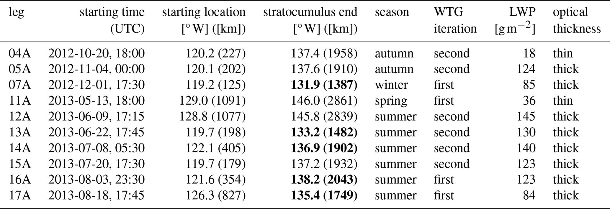
Before we present the results, we provide a short overview of the individual legs, collected in Table 1. As aforementioned, our study contains cases from all seasons including a variety of meteorological conditions. The broad majority of transects was executed in warmer months, where the large lower tropospheric stability leads to a stable situation, in which stratocumulus decks can readily form under a strong inversion (Klein and Hartmann, 1993; Wood, 2012). The third column demonstrates that while most of the cases begin close to the North American coast, three start further offshore than 126° W (or 800 km). Note that the distance in km is the great-circle distance from Los Angeles (LA), which was computed based on the ship's geographical position, and is a solid approximation of the ship's path (Zhou et al., 2015).
In the subsequent analysis, if not stated otherwise, we focus on the stratiform stages where a domain-averaged cloud fraction fc of at least 40 % exists. We chose this particular threshold to eliminate periods of non-existing stratocumulus decks as well as to cut legs that have already completed the transition and have broken up irreversibly. On the grid-scale, fc is binary with either 100 % or 0 %, which is determined by a cloud water mixing ratio threshold of . Note that the cloud water hydrometeors and the rain water hydrometeors in ICON are separated by a mass threshold of . In this study, liquid water content qc, liquid water path (LWP) and the subscript c refer to cloud water, whereas rain water path (RWP) and the subscript r refer to rain water, unless stated otherwise. The final location of the stratocumulus deck in the control runs can be found in the fourth column of Table 1, where legs that transitioned before the end of the simulation are highlighted in bold font. As the fc threshold is applied for each leg individually, this can yield small time periods where one run is still in a stratiform stage, while the other is not. To make the analysis more comparable, we use the more conservative outcome for both runs, as these events occur only infrequently.
We divide all 10 cases into two categories: optically thick (or simply thick) and optically thin (or simply thin), respectively. This classification is based on the amount of liquid water in the cloud deck and targets the blackbody behaviour of a cloud regarding its longwave emissivity. It is well-known that a cloud's longwave emissivity (and thus, its integrated radiative cooling) is approximately constant at LWP ≳ 30–50 g m−2 (e.g. Stephens, 1978; Turner et al., 2007; Williams and Igel, 2021). However, at lower values, this emissivity increases with LWP and so does the radiative cooling that drives stratocumulus development. In the following, LWP denotes the in-cloud liquid water path, which is computed by weighting the domain-averaged liquid water path by the corresponding area cloud fraction based on fc. As summarised in the last two columns of Table 1, eight legs fall in the thick category, while two belong to thin with maximum liquid water paths well below 50 g m−2 in the first 6 h. Note also, that rain water contributes to longwave emissivity in principle, however, its impact is negligible during the early stages of the thin legs (e.g. Fig. 3). For consistency, Table 1 therefore reports LWP without RWP, as including rain water would not affect the outcome.
Table 1Summarised information about the simulated MAGIC legs: The leg numbers, the simulation starting time, the ship's location at the starting time, the final location of the stratocumulus period in the control run depending on whether the simulation ended before the breakup or the cloud deck broke up midway (bold), the season of the transect, the number of WTG iterations performed, the maximum liquid water path (LWP) of the first 6 h of the control run with a horizontal mean cloud fraction of at least 40 %, as well as the resulting optical thickness classification. The locations are given in both longitude and distance from Los Angeles.
3.1 Qualitative evaluation of the deepening evolution
Before we focus on the impact of cloud droplet sedimentation, we will briefly evaluate the quality of our simulations. In doing so, we first compare control runs of two representative legs of each category to MAGIC ship observations regarding inversion height and cloud-base height, and assess the overall development of the SCT. The simulated inversion height zinv in this study is determined by the height of maximum gradient of liquid water potential temperature θl in the boundary layer. It is computed at each time step and each grid cell and averaged over the domain afterwards. The observed inversion height is computed using profiles of potential temperature θ instead of θl, as no condensate was measured in the regular ship radiosonde launches.
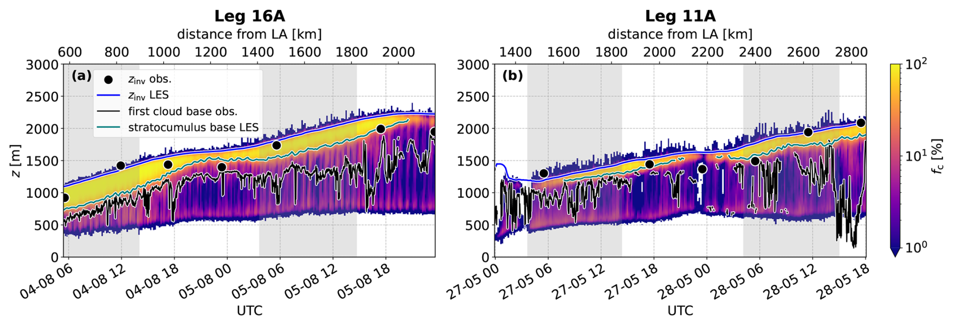
Figure 1Domain-averaged cloud fraction fc of the control runs of (a) Leg 16A and (b) Leg 11A as a function of height z over the course of the simulation. The bottom x-axis marks the respective time of the transect, while the top x-axis marks the distance from Los Angeles. The blue line shows the LES inversion, while the teal line shows the lowest height of fc=40 %, if it exists. The black dots symbolise the observed inversion height based on the ship radiosonde launches (Keeler et al., 2022), whereas the black line depicts the observed first cloud-base based on the ship ceilometer (Zhang et al., 1996). The latter was resampled to a time step of 1 min for better visibility. Grey shading marks local night-time.
Figure 1 depicts the evolution of the domain-mean fc of the thick Leg 16A as well as the thin Leg 11A, excluding the 6 h spinup window. The expected course of the SCT is nicely visible for the thick leg in panel (a). Starting with a low-lying thick stratocumulus deck of high fc, zinv increases continuously, until cloud breakup occurs in the very end. During this process, the stratocumulus deck decouples from the surface and cumulus clouds form below the main deck, indicated by a low fc below the stratiform cloud deck. This behaviour is consistent with the initial stages of the deepening-warming mechanism (Bretherton and Wyant, 1997; Wyant et al., 1997), where the rise in sea surface temperature drives decoupling from the surface. Analogous simulation results for the initial stages of the SCT in MAGIC transects could be obtained by McGibbon and Bretherton (2017) and Zheng et al. (2020). The influence of the diurnal cycle is also identifiable, with episodes of continuous cloud thickening and inversion rise during night-times in contrast to cloud thinning and inhibited growth during day-times during solar insolation. The LES inversion tracks the observed inversion quite well, apart from a bias during day-times, where the inversion seems to decline in the observations. Moreover, the observed first cloud-base from the ship ceilometer (hereafter cloud-base) follows the stratocumulus base relatively steadily in the beginning. Afterwards, it starts oscillating between the stratocumulus base and the underlying cumuli, depending on whether the ship passes under a cumulus cloud or only the stratocumulus deck. Overall, the vertical extension and location of the cloudy layer as a whole is captured well.
In panel (b), the thin Leg 11A is depicted. It is noticeable that the cloud deck is absent at first, forming during the first night. The simulated transect begins more than 1000 km off the coast, leading to an immediately (semi-) decoupled stratocumulus deck with underlying cumuli. The second obvious difference to Leg 16A is the thickness of the deck accompanied by a brief day-time breakup in the middle of the transect. Apart from that, both the deepening process and the diurnal cycle are similar. Furthermore, the observed inversion as well as the observed cloud-base exhibit the same features as in panel (a). They are tracked quite well by the simulated cloud, apart from the day-time bias of the inversion. The cloud-base also shows brief disruption episodes, pointing at the structure of a thinner, more broken-up stratocumulus deck. At the end of the second night, the observed cloud-base drops abruptly to around 200 m, which is not reproduced by the LES. In total, our simulations successfully capture the initial SCT development regarding the deepening of the boundary layer as well as the decoupling from the surface together with the formation of underlying cumuli.
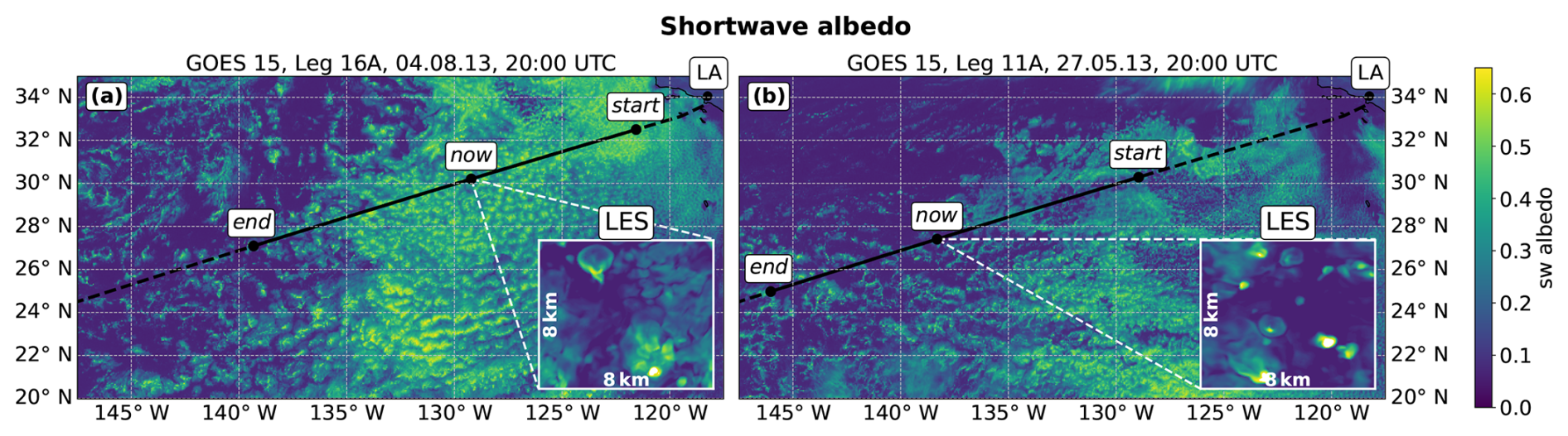
Figure 2GOES 15 broadband shortwave (sw) albedo snapshot of (a) Leg 16A and (b) Leg 11A around midday of the respective day. The dashed black line shows the full MAGIC transect starting from the Los Angeles harbour, while the solid black line shows the simulated part (enclosed by start and end). The midpoint (now) indicates the ship's position during the snapshot. For comparison, the LES pseudo-albedo of this time step is depicted in the small rectangle.
Secondly, we want to evaluate the simulations by comparing them to satellite observations. Figure 2 depicts the domain albedo for the same two representative legs, 16A for thick and 11A for thin. The background plot shows a midday snapshot of the broadband shortwave albedo from the Fifteenth Geostationary Operational Environmental Satellite (GOES 15), obtained using the techniques described in Minnis et al. (2002, 2008, 2011) at a pixel resolution of 4 km. The image during Leg 16A in panel (a) represents a prime example of a subtropical SCT. It is by an extensive, contiguous stratocumulus deck of high albedo, that starts to break up at around 134° W and transitions into free ocean cumuli. In contrast, the cloud deck during Leg 11A in panel (b) is more fragmented, has lower albedo and breaks up earlier. The small embedded rectangle shows the LES pseudo-albedo A of the 8 km by 8 km domain at the time of satellite snapshot, which serves as a proxy for the real albedo. We adopt the approach outlined in Kurowski et al. (2025) based on Meador and Weaver (1980) to include the solar zenith angle. Note that while Fig. 2 only displays a snapshot, we will briefly address the albedo susceptibility in the discussion, where we excluded angles >80° when the sun is located near the horizon. A is computed as
with the ocean albedo αsfc=0.06 and the cloudy albedo Ac. The latter is computed using the individual albedo of a cloudy layer αcld (Stephens, 1984):
Furthermore, we calculate the optical depth τ for αcld using the approach of Stephens (1978):
summing over the individual contributions of cloud and rain water. ρ represents the local air density, represents the density of water, reff and q denote the effective radius and the mixing ratio of the respective liquid hydrometeor. reff is obtained directly from the ICON output (parametrised after Eq. (32) of Seifert and Beheng, 2006). For the sake of brevity, we refer to Appendix A of Kurowski et al. (2025) for the details of the computation of αcld.
The magnitude of the pseudo-albedo largely matches the satellite in both cases. Similarly, both simulation domains capture the qualitative differences in cloud morphology between the two cases described above. The thick Leg 16A case exhibits a broad cloud deck covering most of the LES domain, whereas Leg 11A is far less extensive and features more isolated cumuli, consistent with conditions in the breakup region. In both cases peak albedos inside individual cumuli exceed observed albedo ranges. Furthermore, the simulated cloud deck during Leg 16A seems to be a little more broken than observed. However, it is important to be aware of the scales. The LES domain corresponds to only two by two pixels in the satellite image, which thus (by design) cannot capture any scales of mesoscale organisation. Overall, it is encouraging that the individual simulations exhibit analogous differences to those shown in the satellite images.
3.2 The impact on the inversion height
A common measure for analysing boundary layer growth is the entrainment velocity
originally introduced by Lilly (1968). The calculation involves the change in zinv and the subsidence velocity wsub at the inversion. In the following, we decide against the usage of we in illustrating plots and instead discuss zinv directly. The reason is that we oscillates considerably due to the temporal derivative, requiring substantial smoothing to become interpretable, whereas zinv itself is smooth. However, we continue to use the exact we when comparing changes with values reported in the literature, in order to enable a quantitative evaluation. Qualitatively, variations in zinv mirror those in we, as deviations in the subsidence velocity at the inversion are small between drop_sed and control for the majority of the time, and thus
holds. In the following, all differences Δ are computed as drop_sed − control.
To enable a more compact analysis, we distribute the legs in the two categories as in Table 1. While the optically thin category only consists of two legs, the optically thick one contains eight legs, complicating an individual assessment. Due to their similar behaviour, we opt for a composite analysis in the latter. We use the great-circle distance to Los Angeles for each leg, bin the data in 25 km intervals and then average over all legs in the category in order to acquire one distance-binned dataset. Obviously, the physical interpretation has changed in this setup, as this results in average quantities of all respective transects. However, for our purpose, this is the preferred outcome, since we aim to compare drop_sed and control, which consist of the same transects. Thus, in the subsequent analysis, we deal with averaged quantities in the thick category, while we stick to the two thin legs individually, as also their distance overlap is small.
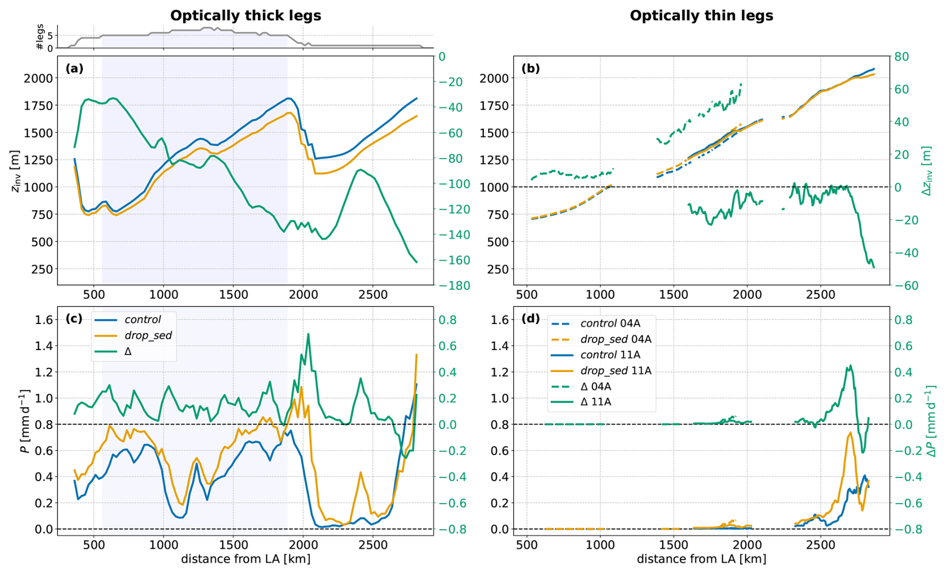
Figure 3Binned distance plots of the inversion height zinv (top panels) and the surface precipitation rate P (bottom panels), separated by category. Panels (a) and (c) represent the thick legs, whereas panels (b) and (d) represent the thin legs. The former are combined into one curve with the leg contribution depicted above the panels in grey, whereas the latter are depicted individually using dashed (solid) lines for Leg 04A (Leg 11A). The left y-axis corresponds to the absolute magnitude of both control (blue) and drop_sed (orange), while the right y-axis corresponds to the difference Δ (green). The light blue shading indicates the core region, where at least five legs are contributing. In all panels save for (b), a rolling mean of roughly 75 km was applied.
The top panels of Fig. 3 show the development of zinv in both categories. In panel (a), the averaged inversion of the eight thick legs follows the expected continuous increase in the direction of the free ocean. However, there are two sharp drops, one in the beginning and another at around 2000 km. Both can be explained by the number of legs contributing to these intervals. The former originates from Leg 07A, being the only leg this close to the coast, but having a relatively high stratocumulus deck, while the latter comes from Leg 12A, which starts very late compared to all other thick legs and has a strong low-lying deck (see Fig. A1). Δzinv is becoming more negative, apart from the very beginning and a considerable period around 2300 km, indicating reduced entrainment in the drop_sed runs. While the initial increase is an artifact of the averaging procedure, when new legs are added (cf. the distribution above panel (a)), the sharp increase in the later stage is a distinct feature of Leg 12A, which will be discussed in Sect. 4.1. The increasing negative divergence in the core region between 550 and 1900 km (indicated by the blue shading) corresponds to a mean reduction in we of around 9 %, which is in good agreement with previous studies. The non-precipitating LES studies of Bretherton et al. (2007) and Hill et al. (2009) yielded a reduction in we of around 7 %, while Ackerman et al. (2009) reported a decrease of up to 25 % in their precipitating case. de Lozar and Mellado (2017) and Pistor and Mellado (2025) found even stronger reductions of 20 % to 50 % in their DNS, as these simulations generally observe more pronounced effects through their fine resolutions. It is important to acknowledge that the present value of 9 % is an average over different transects and also includes diurnal cycle effects, while the other LES studies consist of one specific case in nocturnal conditions. Here, we observe individual periods of reduced entrainment that can be as large as 20 % in precipitating cases, consistent with Ackerman et al. (2009).
In contrast, the thin cases in panel (b) show a different behaviour. While the development of the deepening boundary layer is the same for both Leg 04A (solid) and Leg 11A (dashed), the behaviour of control compared to drop_sed differs crucially. For Leg 04A, Δzinv is constantly increasing after 1000 km, implying that entrainment is enhanced in the drop_sed run. In this case, this even leads to a 60 m deeper boundary layer at the end of the simulation. In this period, a mean entrainment amplification of 10 % is observed, which is of comparable magnitude to the previously reported reductions in LES studies. For Leg 11A, this effect is not as pronounced, but still noticeable. The inversion in the drop_sed run starts roughly 10 m below the control one after the delayed cloud formation (cf. Fig. 1b). After a brief increase of this deviation, the trend is a slow, but steady decrease, which can be quantified to a mean entrainment amplification of 2 % in the drop_sed case. As soon as Δzinv reaches 0 m, an abrupt drop occurs, that can be attributed to the sudden formation of drizzle (cf. panel (d), details in Sect. 4.2). To our knowledge, enhancement of entrainment in stratocumulus due to cloud droplet sedimentation has not been reported before.
The bottom panels of Fig. 3 depict the corresponding precipitation rates in both categories. The thick cases in panel (c) develop relatively strong precipitation throughout the majority of the transects, which is comparable to the heavy drizzle rates of 1 mm d−1 in Stevens et al. (1998) and Savic-Jovcic and Stevens (2008). The reason for the seemingly lower values and the oscillatory behaviour is the averaging over multiple legs, leading to a mix of day-time and night-time. It is evident that the precipitation rates are considerably increased in the presence of droplet sedimentation, in accordance with Ackerman et al. (2009). In contrast, the precipitation rates of the thin cases in panel (d) are very small. Leg 04A develops almost no surface precipitation at all, independent of the type of simulation. Leg 11A also shows very limited precipitation, apart from the final stage of the simulation, where a sharp enhancement can be observed. This increase is greatly reinforced in the drop_sed case, directly affecting zinv in panel (b). From that, we can conclude that precipitation is a strong factor in the boundary layer development of the present cases.
3.3 The turbulence feedback mechanism
The observations from the previous section raise two main questions. First, how can droplet sedimentation lead to enhanced entrainment and second, why does this predominantly occur in the thin legs. In this section we aim to disentangle the primary process chain by examining the temporal evolution of the sedimentation effect in two stages: the short-term effect in the initial hours and the long-term effect afterwards.
Sedimentation acts to remove cloud water from the cloud-top layer and thereby reduces evaporation. This reduction in evaporation impedes entrainment and directly leads to an increase in LWP (Bretherton et al., 2007; Wyant et al., 2007; Ackerman et al., 2009; Pistor and Mellado, 2025). The initial reduction in entrainment is visible in all our simulations, not only the thick ones, but also the thin ones. To quantify this, we computed the mean Δzinv in the hours 2 to 5 for each leg, except Leg 11A, where we used the hours 13 to 16 due to the delayed cloud formation. This way, we discard only the two initial hours as spinup, after which the simulations have mostly stabilised. For Leg 04A, the reduction occurs mainly in the first 4 h, which is not displayed in Fig. 3 due to the discarded spinup window of 6 h. To verify that the observed effect is not an artifact of model spinup, we conduct another simulation for this leg. In doing so, we start with the control settings, but activate droplet sedimentation after 15 h and let the simulation evolve until the end. We chose this particular activation time step, as the cloud deck's properties such as thickness or LWP, are comparable to the initial hours. A plot for the resulting zinv for Leg 04A can be found in the appendix Fig. A2.
Table 2Leg-wise mean quantities of the first 3 h after cloud formation, excluding 2 h of spinup. The first row shows the inversion height zinv, whereas the second row shows the mean cloud-top height zct, with the results for the spinup experiment of Leg 04A in brackets. The third (fifth) and fourth (sixth) row represent the liquid (rain) water path (LWP; RWP) and its difference Δ, respectively, while the last row lists the sedimentation velocity vsed,75 of the drop_sed run in the 75 m below zinv. Recall that for all variables x.
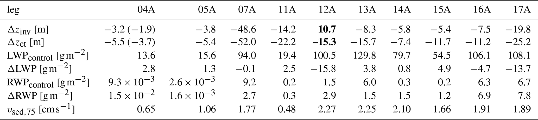
The results for all legs are summarised in Table 2 with the sensitivity result for Leg 04A in brackets. The first two rows present the difference of two measures for the stratocumulus top: zinv and the mean cloud-top height zct. The latter is calculated from the maximum height of the cloud water mixing ratio in each column (Ackerman et al., 2009) and is averaged over the domain afterwards. It serves as an additional tool to check if zinv behaves as expected in the initial hours of the simulation. Note that Δzct evidently leads to larger differences than Δzinv, as it is directly driven by the sedimenting droplets. Both approaches yield an overall negative difference for all legs, apart from Leg 12A (marked in bold), confirming the reduced entrainment in the initial hours. For Leg 12A, only zct confirms the reduced entrainment, whereas zinv disagrees. However, in this case, the thermodynamic inversion clearly does not fit to the top of the cloud in the early hours of the simulation (cf. Fig. A3), which is further indicated by its actual high sedimentation velocity. Considering this, we conclude that also in this case, entrainment is indeed reduced in the initial hours.
Regarding the sedimentation velocity, it is clear that legs with a low initial LWP also have substantially lower sedimentation velocities due to their smaller effective radii. Comparing LWP control to the LWP in Table 1, it is noticeable that some of the optically thick legs (especially Leg 05A and Leg 15A) would be categorised as optically thin. However, this is simply an artifact of the initial cloud formation, that vanishes shortly. The expected increase in LWP in the drop_sed runs (i.e. positive ΔLWP values in the fourth row) is not observed uniformly for all legs. Instead, a decrease is observed for the legs 07A, 12A, 16A and 17A. However, taking into account the change in RWP in the sixth row, this deviation can be readily explained by the considerable amplification of rain water in these cases. The excess is at least 2.7 g m−2, while the other legs have a maximum excess of 1.5 g m−2. The rain water depletes the cloud by collecting droplets and removes them through precipitation, which is enhanced in drop_sed by the sedimenting cloud droplets (Ackerman et al., 2009). In the other cases, this enhancement does not (yet) dominate and thus, the reduction in entrainment yields an increase in LWP.
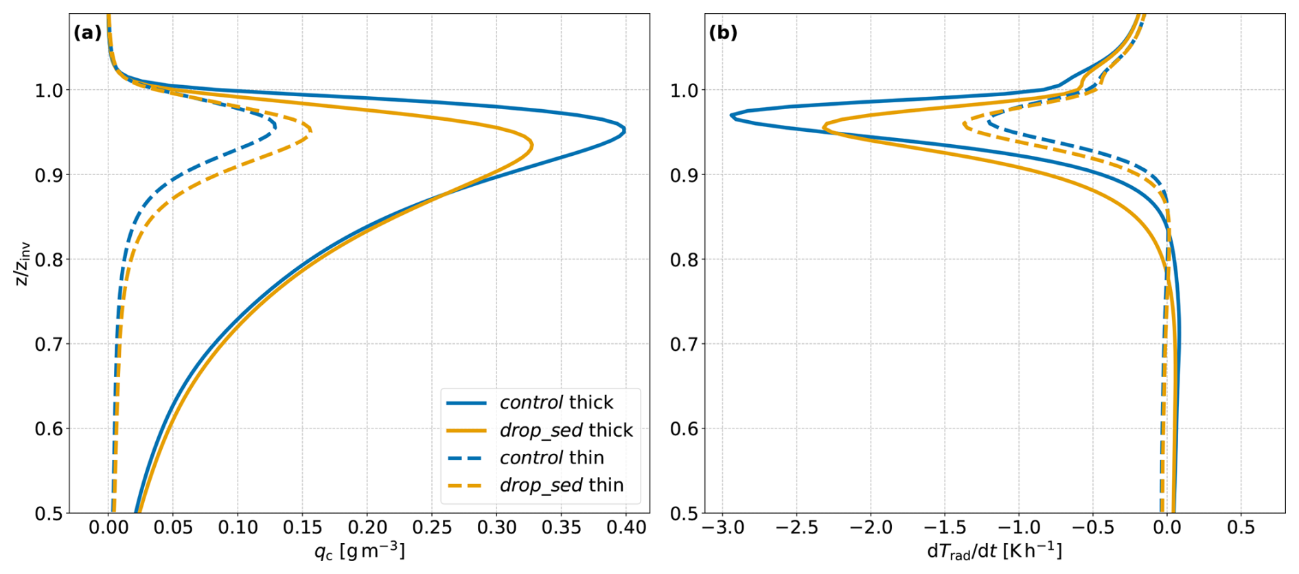
Figure 4Total mean relative profiles of (a) liquid water content qc and (b) radiative heating rate . The profiles were normalised to the inversion height zinv at each time step before computing the mean. The thick (thin) legs are represented by solid (dashed) lines. Note that the y-axis is cut at 0.5. Colours as in Fig. 3.
So far, we have seen that the initial stages indeed yield the expected reduction in entrainment accompanied by an increase in LWP, if the simultaneous increase in RWP is not too strong. Rain formation in general is obviously crucial, as drizzle in stratocumulus can have a substantial effect on boundary layer dynamics by, among other things, depleting the cloud of liquid water or reducing turbulent kinetic energy (TKE) (e.g., Stevens et al., 1998; Savic-Jovcic and Stevens, 2008). For now, we will restrict our analysis to the general cases, but we will treat the impact of precipitation in a sensitivity experiment in Sect. 4.2.
Next, we focus on the impact of sedimentation after the initial period, continuing with the amount of liquid water in the cloud. Figure 4 shows the mean relative qc profile, as well as the mean relative radiative heating rate profile, split up into the two categories. These profiles (and all subsequent ones) were obtained as follows: For each leg at each time step after the 6 h of spinup, the height coordinate was normalised by the corresponding zinv. After that, the corresponding legs were merged and a normalised mean profile over all time steps was computed in both categories. Starting with the thick legs, the decline in LWP, which was already foreshadowed in Table 2, is also visible in the overall mean in panel (a). The stratocumulus region around the maximum of the profile shows a clear decrease, while there is a slight increase in the sub-cloud areas in the drop_sed runs. Moreover, the maximum also dropped considerably due to the sedimenting droplets. In contrast, the thin legs retain and even amplify their initial liquid water increase throughout the entire cloud layer. One reason behind that is the lack of drizzle in the thin cases, which only only forms towards the end of the simulation in both legs (cf. Fig. 3d), and thus, does not drain the cloud of liquid water.
This behaviour is also reflected in the radiative heating rate in panel (b). The peaks in both drop_sed curves have shifted to lower relative heights. In the thick cases, the peak cooling rate declined substantially. However, most of it was simply transferred to lower heights, where a comparable strengthening can be observed. In contrast, the thin cases show an amplification in longwave cooling across the full cloud layer, consistent with the qc profile in panel (a). The reason for the overall increase, instead of a shift as for the thick legs, is the LWP dependence of the longwave cooling, which was the mean criterion for our categorisation in Sect. 2.4. For the thin legs, an enhancement in LWP still leads to an enhancement in integrated longwave cooling, which is why the cooling rate is amplified across the entire layer (Stephens, 1978; Turner et al., 2007).
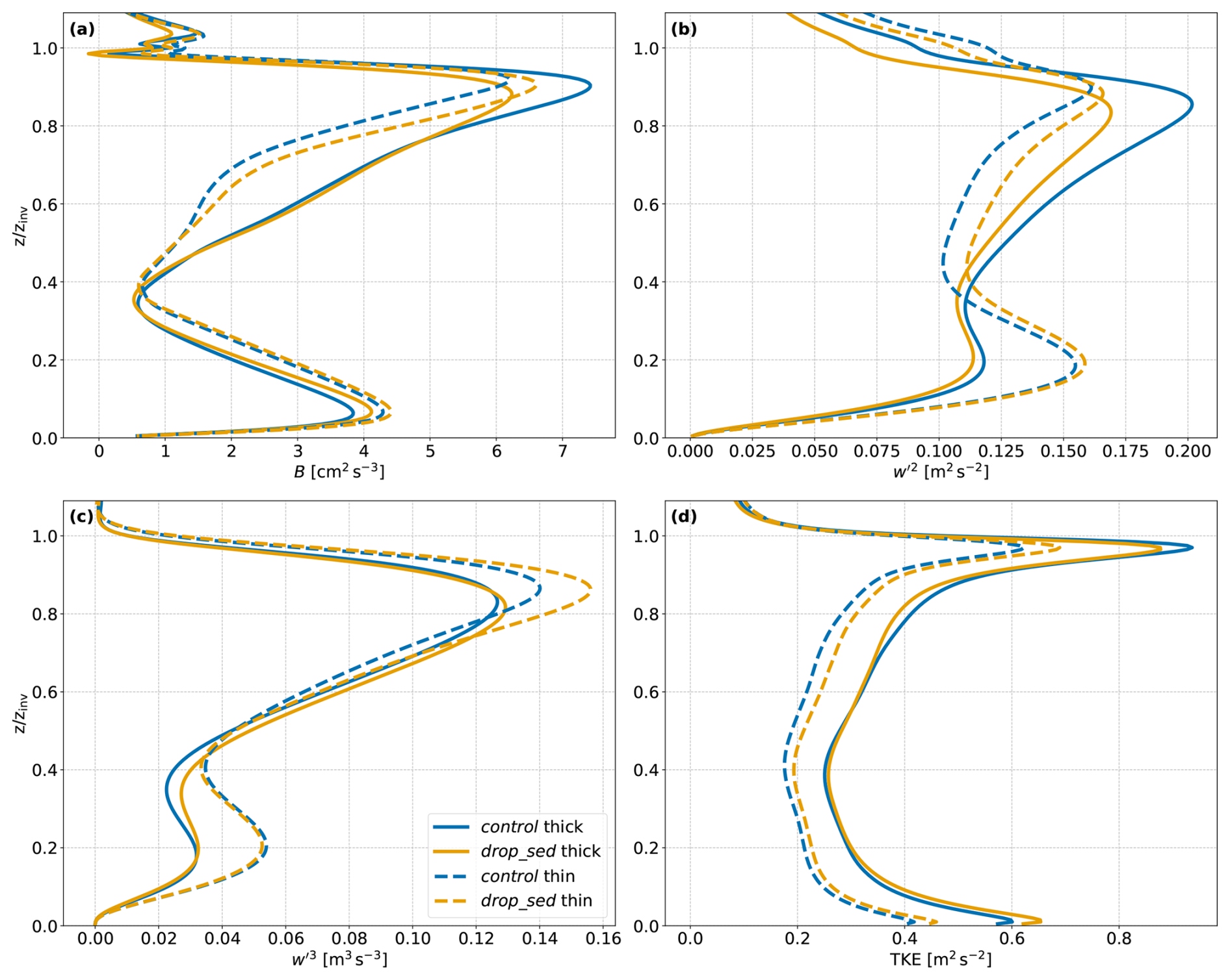
Figure 5Total mean relative profiles of the (a) buoyancy flux B, (b) vertical wind variance , (c) third moment of the vertical wind and (d) turbulent kinetic energy (TKE). Lines and colours as in Fig. 4.
Figure 5 presents analogous profiles of selected turbulence quantities. In the thin case, the overall increased qc, combined with enhanced longwave cooling, is expected to amplify turbulent circulations in the boundary layer (e.g. Feingold et al., 2015). Panel (a) shows the buoyancy flux, which is indeed enhanced in the drop_sed case throughout the cloud layer, while it remains relatively unchanged below. In contrast, the thick legs exhibit the opposite behaviour. Buoyancy production is considerably decreased in the upper cloud layer and relatively constant elsewhere, apart from an increase near the surface. The former decrease can be attributed to several stabilising factors. The removal of liquid water from the top due to the rain yields not only a decrease in longwave cooling, but also in latent heat release and less cloud-top evaporation overall. Both categories consistently display a minimum buoyancy of around 0.5 cm2 s−3 in the sub-cloud layer, which is characteristic of the decoupling process, that occurs during the course of the SCT. Note that while no full buoyancy flux reversal is visible, this is a mean profile of eight cases over a period of 42 h. Full individual decoupling represented by negative buoyancy fluxes does in fact occur in the later stages of the simulation of each leg.
The corresponding minimum is also apparent in the vertical wind variance in panel (b), although less distinctive in the thick category. The same overall observations can be made here. While the thin legs show an increase in across nearly the entire boundary layer, the thick legs display a consistent decline in , indicating that turbulence is increased in the former and reduced in the latter. Comparing the profiles of and qc in Fig. 4, they follow the same trend. In the thin cases, both quantities increase, while in the thick cases, both quantities decrease in the stratiform cloud layer. This correlation between qc and in the presence of cloud water sedimentation was also found in other studies. Bretherton et al. (2007) and Pistor and Mellado (2025) simulated a non-precipitating, low-LWP case and observed an enhancement of both qc as well as , aligning with the results of our thin cases. On the other hand, Ackerman et al. (2009) found a qc profile similar to that of our thick cases, along with a reduction in in their drizzling, high-LWP simulation. This resulted in an overall increased LWP, in contrast to the LWP reduction in our thick cases. However, this apparent contradiction can be resolved by the respective amounts of precipitation. In the case of Ackerman et al. (2009), surface precipitation was around 0.2 mm d−1, while almost all of our thick legs reach precipitation rates of , consistent with the magnitude of Stevens et al. (1998) and Savic-Jovcic and Stevens (2008). This much stronger precipitation quickly overwhelms the initial LWP increase, resulting in both reduced LWP and .
In panel (c), the third moment of the vertical velocity is depicted. While the second moment of the vertical wind characterises the strength of turbulent fluctuations, the third moment describes the asymmetry between upward and downward motions. Positive (negative) indicates strong and narrow updrafts (downdrafts), in the presence of generally weak and broad downdrafts (updrafts). For both categories, is consistently positive throughout the boundary layer, implying that there is an overall weak subsidence disrupted by narrow updrafts. In the thin cases, it increases in the presence of cloud droplet sedimentation across the cloud layer, pointing at even stronger, more concentrated updrafts. Together with , we can confidently say that in drop_sed, stronger updrafts drive vertical motions in the cloud. In contrast, is only slightly enhanced in the thick cases, and even unaffected in the upper levels of the cloud.
The full resolved TKE profile is presented in panel (d). The sub-grid scale contribution is small and exhibits the same behaviour, which is why it is omitted here. All profiles show the characteristic peaks near the inversion and at the surface, where the impact of shear is the strongest. Overall, it reinforces all our observations regarding control and drop_sed from before. In the thin cases, the TKE is considerably increased in the entire boundary layer. In contrast, it is decreased in the cloud layer in the thick cases and slightly enhanced towards the surface.
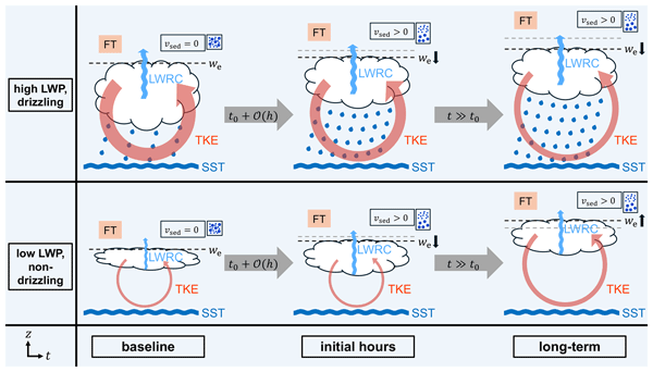
Based on these previous findings, we can construct the following process chain to explain the differences in entrainment outcomes among the two categories in the presence of sedimentation. In the initial stages, cloud droplet sedimentation leads to the expected and often observed result in all cases: entrainment is lowered, as droplets are removed from the inversion layer, reducing the potential for evaporative cooling. Accordingly, this is accompanied by an increase in LWP. After this initial period of a few hours, the individual cases split.
In the heavily precipitating optically thick cases, the trend of reduced boundary layer growth continues, as droplet sedimentation enhances rain formation. Rain acts to lower convective intensity, as latent heat release near the top and latent heat consumption below cloud-base impede turbulent circulations. Furthermore, it drains the cloud of liquid water, which overwhelms the initial increase in the present cases. Thus, the initial weaker boundary layer growth is amplified and continues until the end of the simulation (or the breakup of the cloud deck).
In the optically thin cases without strong precipitation, neither the TKE reduction nor the liquid water depletion occurs. Rather, the initial LWP increase induces additional longwave cooling, which is not yet saturated due to the small overall LWP. This leads to more potent turbulent circulations in the boundary layer, especially stronger and narrower updrafts, that can redistribute moisture from the ocean surface and thereby enable more liquid water production. This turns into a feedback loop of more liquid water leading to more cooling leading to more turbulence leading to more liquid water, that counteracts the weak stabilising effect of rain. Since the sedimentation velocities in the thin legs are low due to their small effective radii, the additional turbulence is able to transport liquid water all the way to cloud-top. This re-enables stronger evaporative cooling, which, in combination with the longwave cooling, adds to the total cooling. As long as rain formation remains limited and the LWP is small enough for the radiative cooling to be unsaturated, this turbulence intensification prevails. Altogether, the enhanced convective intensity, supported by the evaporative cooling, promotes stronger entrainment and allows it to persist over an extended period of time.
In our proposed mechanism, we identified drizzle formation as well as the amount of liquid water with regard to longwave cooling as the two crucial drivers. We now want to test the robustness and importance of these factors during individual periods as well as additional sensitivity experiments.
4.1 Leg 12A, optically thin period
The previous investigations involving the averaged profiles evidently resemble overall behaviour, however, certain periods of individual deviations can be shadowed. Since we simulate two full days, the effect of the diurnal cycle is included in our runs. Especially the day-time thinning of the cloud deck in the thick legs can have a profound impact on the LWP, and also potentially shift the leg from the thick to the thin category. One example, which is even visible in panel (a) of Fig. 3, is the period between 2200 and 2400 km. Here, the continuous decline of Δzinv is interrupted by a period of strong increase, indicating enhanced entrainment. As evident from Table 1, only Leg 12A contributes this far off the coast, implying this is an individual feature of this leg, that we can analyse.
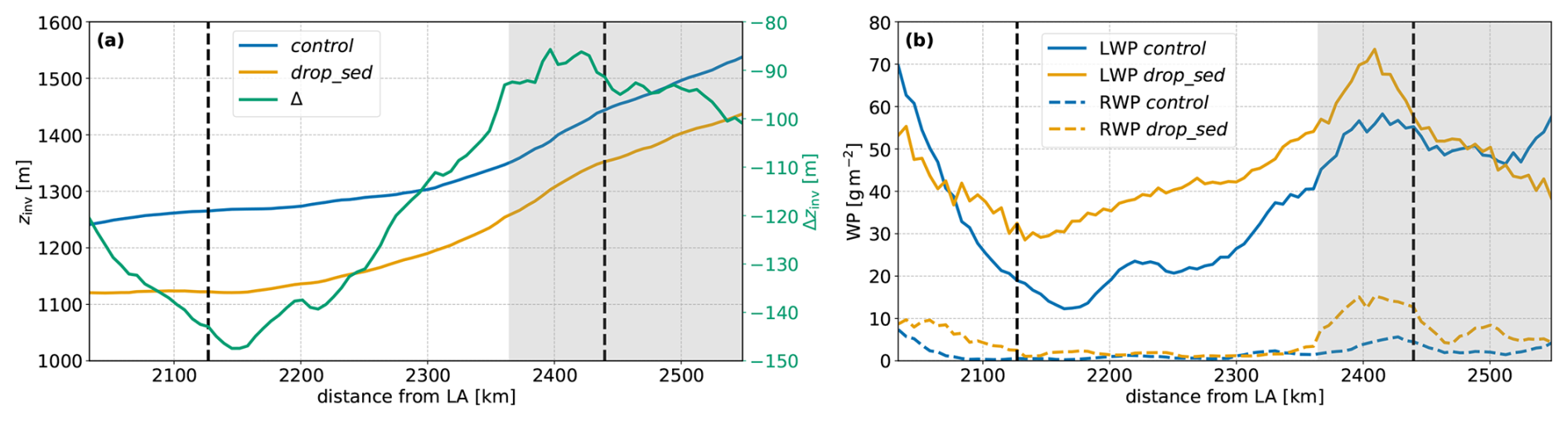
Figure 6Time evolution of the (a) inversion height zinv and (b) water paths (WP) of Leg 12A in the hours 26 to 40 of the simulation. The vertical dashed lines enclose the analysis period for this section. In panel (b), the solid lines depict the liquid water path (LWP), while the dashed ones depict the rain water path (RWP). For the water paths, a 1 h rolling mean was applied. Colours as in Fig. 3 and grey shading marks local night-time.
For clarification, we displayed zinv of Leg 12A in this time period in panel (a) of Fig. 6. The vertical dashed lines mark the interval of increased entrainment in the drop_sed run, that we analyse in the following. We decided to extend this interval a little further than the extremes to also capture the initial and final stages more accurately. The steady increase between the two extremes of Δzinv corresponds to a mean acceleration of we of 18 % over the course of 7 h. This acceleration is not only substantially larger than the previous amplification of around 10 % in the case of Leg 04A, but also in the vicinity of the strongest individual reduction of an individual leg of around 20 %. In panel (b), both LWP and RWP in this period are depicted. The overall amount of LWP is well within the range, where longwave cooling is not saturated, until the beginning of the second night. The low values are the result of the day-time thinning through solar insolation. The RWP declines simultaneously and arrives at almost no rain at the start of the chosen interval. While the LWP was larger in the control run before, this flips and reaches values more than twice as high in the drop_sed run. At the end of the day, the overall magnitude of the LWP increases again, supporting the rain formation in drop_sed. As soon as the RWP is substantially increased in drop_sed, the corresponding LWP declines and becomes once again lower than in control, marking the end of the interval.
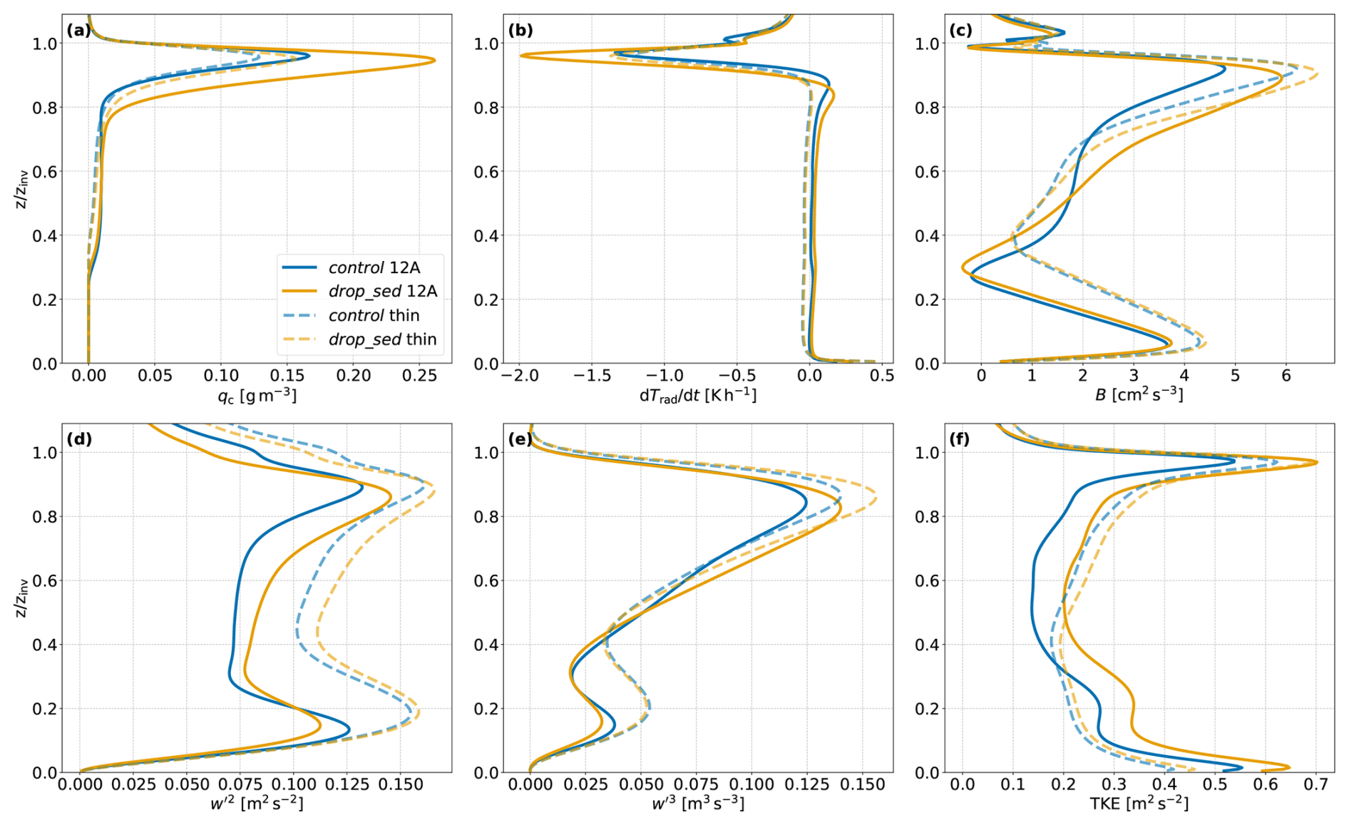
Figure 7Total mean relative profiles of the (a) liquid water content qc, (b) radiative heating rate , (c) buoyancy flux B, (d) vertical wind variance , (e) third moment of the vertical wind and (f) turbulent kinetic energy (TKE). The solid lines represent Leg 12A in the thin period, while the transparent dashed lines represent the full thin profiles for comparison. Colours as in Fig. 4.
Following the analysis in Sect. 3.3, Fig. 7 shows the different relative profiles. The solid lines represent the relative profiles for Leg 12A in the selected period marked by the dashed vertical lines in Fig. 6. Furthermore, we added the full thin profiles from Figs. 4 and 5 in fainter dashed lines as a reference. Without repeating the details regarding individual profiles, it is evident that all six Leg 12A profiles behave analogously to the thin cases. During this period, qc, longwave cooling as well as the turbulence quantities are considerably increased. Especially the former two show an even stronger amplification for Leg 12A than for the thin legs, which is possible thanks to the absence of rain. This leads to a pronounced increase in TKE throughout the entire boundary layer, promoting entrainment in the drop_sed run. These results firmly support the proposed feedback loop from Sect. 3.3, confirming that enhanced longwave cooling is a main driver in regions of low LWP. Furthermore, this demonstrates that the categorisation into optically thick and optically thin is not rigid. Especially initially thick legs can become thin over the course of one diurnal cycle, when solar insolation dries out the cloud deck during the day (as we saw here for Leg 12A), highlighting the importance of the diurnal cycle in the context of the SCT.
4.2 Non-precipitating cases
In order to further evaluate the proposed mechanism, we conduct three more sensitivity experiments, the first one targeting precipitation. Precipitation in stratocumuli has a profound impact on boundary layer dynamics. Stevens et al. (1998) showed that heavy drizzle substantially reduces entrainment through a reduction in turbulent kinetic energy. As drizzle forms, latent heat is released in the cloud through condensation, warming the cloud layer. When the rain drops sediment out of the cloud, evaporation leads to cooling in the sub-cloud layer. This combination restrains deep circulations and supports the formation of cumuli below the original stratocumulus deck. These results were largely confirmed in the large-domain LES study by Savic-Jovcic and Stevens (2008), where also a reduction in TKE as well as boundary layer growth was observed in the presence of strong drizzle.
In our simulations, all optically thick cases are strongly drizzling for a certain period of time, whereas only very limited drizzle forms in the optically thin ones. This can be directly attributed to the differences in the amount of liquid water in the clouds. The surface precipitation rates for the representative legs can be found in panels (a) and (b) of Fig. 8, respectively. Leg 16A features substantial drizzle rates from the beginning, with a considerable drop during the first day due to the day-time thinning of the cloud deck. Moreover, in the drop_sed runs, precipitation formation is generally enhanced because of the sedimenting droplets, which was also observed by Ackerman et al. (2009). In contrast, Leg 11A only develops a sizeable amount at the end of the second night, which is again substantially larger in the drop_sed run. This strong increase is also responsible for the abrupt drop in the drop_sed inversion shown in panel (d), since the rain drops not only reduce the available TKE, but also simply deplete the cloud of liquid water (Stevens et al., 1998; Savic-Jovcic and Stevens, 2008; Ackerman et al., 2009).
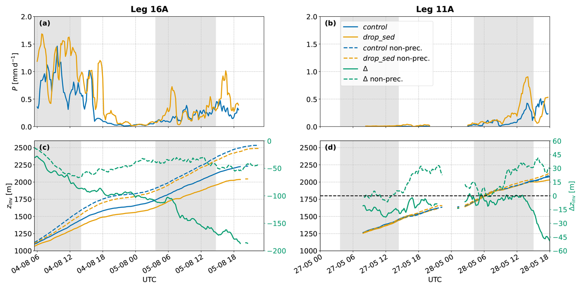
Figure 8Comparison of the representative legs for the thick category (Leg 16A, left) and thin category (Leg 11A, right). The top panels (a) and (b) show the surface precipitation rates P, while the bottom panels (c) and (d) show the results for the inversion height zinv, respectively. For the precipitation rates, a 1 h rolling mean was applied. The solid lines represent the precipitating runs, whereas the dashed lines represent the non-precipitating runs. Colours are the same as in Fig. 3 and the grey shading marks local night-time.
To rule out the possibility that the absence of drizzle alone is responsible for the observed behaviour in the thin cases, we performed two non-precipitating sensitivity runs for the representative legs. The resulting zinv together with the precipitating runs can be found in the bottom panels (c) and (d) of Fig. 8. Comparing the impact during Leg 16A, there is a clear difference after the first night. While the precipitating case shows only a weakened divergence in Δzinv during the first day, the non-precipitating case actually shows a weak, but continuous, enhanced boundary layer growth in the drop_sed case. After this period of faster growth, it roughly stabilises until the end, leading to an overall lower boundary layer in the non-precipitating drop_sed run. So after the strong initial decrease in entrainment, Δzinv in the non-precipitating runs remains similar, with periods of slightly increased or reduced boundary layer growth. This reflects the counteracting effect of the sedimenting droplets and the enhanced turbulence, where the latter is now not affected by precipitation. During the stronger entrainment phase, there is a lot more liquid water near cloud-top (cf. Fig. 10b, green line) leading to enhanced evaporative cooling and thus, stronger turbulence in the entrainment zone. Furthermore, during the day, the LWP drops substantially into the regime of unsaturated longwave cooling, while still being considerably enhanced in drop_sed (cf. Fig. A4). This way, the overall cooling is not only redistributed, but also magnified and the amplified turbulence can work against the sedimenting droplets. After that period, the sedimentation balances out the increased turbulence, as the cloud enters the thick regime during the second night again and cloud water is not longer enhanced in the cloud-top region. This situation can be seen as an unstable equilibrium of the sedimenting droplets reducing entrainment and the enhanced LWP counteracting it by amplifying turbulent circulations.
For Leg 11A, the situation is different. Both runs commence around the same zinv, followed by two episodes of strongly increasing Δzinv, with an intermission of decreasing Δzinv. So even though almost no drizzle drops are present in the beginning, the inclusion of rain processes alters the base state of the stratocumulus deck. Furthermore, the lack of rain enables even faster entrainment in the drop_sed case until the middle of the first day, after which solar insolation dries out the deck. The fact that the control inversion grows faster in this period might by a consequence of the almost vanishing cloud. After the reformation is complete, drop_sed entrains faster again, resulting in a net raised cloud-top height after the full 48 h.
In summary, the overall impact of precipitation can mask and overwhelm the enhanced entrainment effect of sedimentation in the thin cases, if substantial amounts of drizzle form. However, we can infer from the analysis of Leg 16A, that even though drizzle plays a large role in reducing entrainment, it is not solely responsible for reduced entrainment in simulations with activated cloud droplet sedimentation. Rather, sedimentation reinforces drizzle that decreases entrainment, while the non-precipitating thick case shows that the additional liquid water can balance out the original sedimentation-entrainment feedback after the initial period. In contrast to the consistent entrainment increase in Leg 04A, this outcome is unstable, since it lacks the amplification of longwave cooling as an additional driver of turbulence.
4.3 Optically thin case with low background CCN
The second sensitivity experiment examines the influence of the CCN background in the individual transects. CNN are among the important factors regulating precipitation onset, as the amount of cloud droplets is directly dependent on the number of CCN. In general, higher CCN concentrations yield more and smaller cloud droplets and thus, thicker clouds (e.g., Twomey, 1977; Twomey et al., 1984; Albrecht, 1989). In the Northeast Pacific, the CCN concentration declines towards the open ocean, as the influence of continental pollution diminishes. This westward decrease has also been observed during the MAGIC campaign (Painemal et al., 2015; Brendecke et al., 2022). As mentioned in Sect. 2.1, we used a background CCN concentration of 250 cm−3 for all legs, which is a solid approximation for the thick legs in our 48 h window (Painemal et al., 2015). Apart from Leg 12A, these simulations either terminate or the stratocumulus deck breaks up no later than 138.2° W (cf. Table 1). However, for parts of Leg 04A and especially for Leg 11A, this value exceeds the acceptable range. The latter leg starts outside the continental influence and is further a low CCN leg (Painemal et al., 2015). To address this issue, we repeated the Leg 11A runs with the ICON maritime setting of a background CCN concentration of 100 cm−3. We did this both in the precipitating and the non-precipitating setup to observe possible changes in both cases. Before discussing the results, it is worth noting that CCN concentrations are not the primary driver behind the observed thick and thin categories. The likely more important drivers are large-scale synoptic conditions impacting temperature and humidity. Most of the thick legs form under a strong inversion with cold and moist inflow from the North. In contrast, this inflow is considerably attenuated in the thin legs, yielding thinner cloud decks with weaker inversions.
The resulting zinv can be found in Fig. 9. The precipitating case shown in panel (a) exhibits a similar evolution in the low CCN scenario with a weaker growing zinv in the drop_sed case. However, on closer inspection, the period of continuously stronger entrainment during the first day in the drop_sed case of the standard CCN scenario is not distinctly present in the low CCN one. Rather, an overall weaker growing boundary layer with brief intermittent bursts of stronger entrainment is observed, resulting in a decreasing trend of Δzinv. It can also be seen from the disappearance of the dashed line in the second night, that the cloud fraction of the stratocumulus deck drops below 40 % and does not recover until the end. This development can be explained by the altered precipitation behaviour. The maximum drop_sed surface precipitation rate of below 1 mm d−1 is reached at the end of the second night in the standard CCN scenario (cf. Fig. 8b). In the new experiment, this value is surpassed at the beginning of the second night and increases up to almost 1.5 mm d−1 in both control and drop_sed (not shown). The lower CCN concentrations facilitate rain formation due to the larger droplets, which is in accordance with earlier findings from e.g. Feingold et al. (1999). The resulting strengthened decoupling leads to the observed reduced boundary layer growth in the low CCN scenario. Additionally, the continuous negative divergence of Δzinv can be explained by the overall enhanced rain formation in the drop_sed case. As for the thick legs, the reinforcement of rain in combination with the sedimenting droplets is stronger than the amplified turbulence and we observe overall less entrainment. It should be noted that this effect is less pronounced than during the thick legs, because drizzle formation is still suppressed in the beginning due to the low overall LWP. Thus, the latter is still periodically enhanced in drop_sed and the resulting stronger circulations can (partially) balance out the slow sedimentation velocity combined with the weak drizzle.
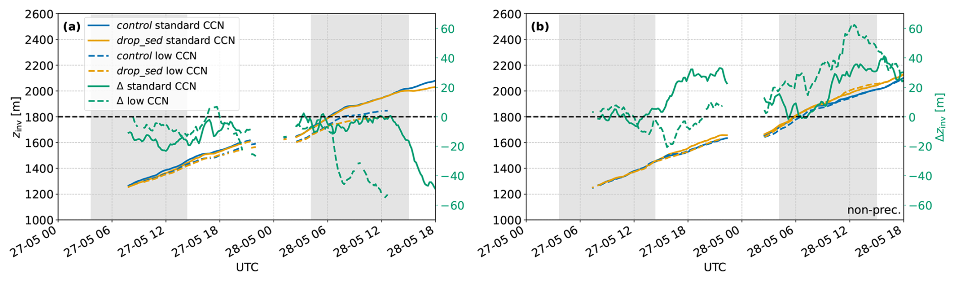
Figure 9Inversion heights zinv of the (a) precipitating and (b) non-precipitating low CCN sensitivity experiments for Leg 11A. Colours and shading as in Fig. 8. The solid lines represent the standard CCN scenario (250 cm−3), while the dashed lines represent the low CCN scenario (100 cm−3).
In the non-precipitating scenario of the different CCN cases in panel (b), the dashed blue and orange lines remain close to the solid ones, in contrast to panel (a). This is because rain is absent and cannot interfere with the cloud dynamics, which leads to a very similar development of the dashed and the solid curves. Comparing Δzinv, the evolution of the dashed and the solid line is slightly different. Instead of the exchanging periods of increased and decreased entrainment, there is an initial decline in entrainment in the drop_sed run, followed by a continuous amplification and a final decline. While less CCN clearly influence the quantitative cloud development, the overall stronger entrainment in the drop_sed run, even leading to a deeper boundary layer, remains unchanged.
In general, we can conclude that the low CCN scenario does not yield structurally different outcomes. It slightly modified the course in the non-precipitating setup and reinforced drizzle formation in the precipitating one. This does produce a considerably different outcome in the latter, but this is not in conflict with our proposed process chain. It rather shifts this leg into the regime, where precipitation-induced stabilisation additionally works against the enhanced turbulence feedback loop and takes over earlier.
4.4 Optically thick case with reduced sedimentation velocity
The last sensitivity experiment targets the magnitude of the sedimentation velocity. As sedimentation reduces entrainment, higher sedimentation velocities should evidently lead to a stronger reduction (Bretherton et al., 2007; Ackerman et al., 2009; Pistor and Mellado, 2025). Table 3 summarises the mean cloud droplet sedimentation velocities in the top 75 m of the representative legs. For Leg 11A, vsed,75 is about two thirds of Leg 16A in the precipitating case, and half of it in the non-precipitating case. As the cloud in the non-precipitating Leg 16A run contains much more liquid water (cf. Fig. A4), the effective radii are larger and the sedimentation velocities are higher compared to the precipitating case. In contrast, Leg 11A lacks this feature, as there is almost no precipitation anyway. In general, the thin cases have substantially smaller sedimentation velocities due to their lower effective radii.
Table 3Mean cloud droplet sedimentation velocities vsed,75 in the 75 m below the inversion over the whole course of the individual transects. The subscript vsed refers to the sensitivity experiment where the sedimentation velocity was halved.

To emulate the impact of the sedimentation strength of an thin leg on a thick leg, we conducted two sensitivity runs (precipitating and non-precipitating) for Leg 16A. In these simulations, we artificially halved the sedimentation velocity in the ICON microphysics. The resulting mean sedimentation velocity can be found in the respective third columns of Table 3. Clearly, the manual scaling by a factor of 0.5 does not yield a precise halving of the individual sedimentation velocities, as this introduces additional feedbacks. However, on average, the overall mean reduction is around 50 %, which is similar or even smaller than vsed,75 of Leg 11A.
Panel (a) of Fig. 10 shows the corresponding Δzinv, that are each calculated with the respective control run (i.e. either precipitating or non-precipitating). Comparing the precipitating cases, the reduced sedimentation difference (orange) follows the same course as the original one (blue). On closer inspection, it is noticeable that this remarkably occurs at almost exactly half the value for the entire transect. Similarly, the precipitation rate differences (dashed) are also roughly halved, confirming the direct impact of vsed on drizzle production (Ackerman et al., 2009). This further implies that, even in the case of lower sedimentation speeds, drizzle dominates boundary layer deepening in the thick cases and yields a constantly slower boundary layer growth rate. However, the amount of drizzle production seems to be directly determined by the sedimentation velocity. The drizzle dominance is also visible, when comparing the precipitation curves to Δqc,75 in panel (b). All four main periods, where blue is clearly above orange in the former, largely coincide with an inverse behaviour of the latter. This is the direct effect of strong drizzle depleting cloud-top of liquid water.
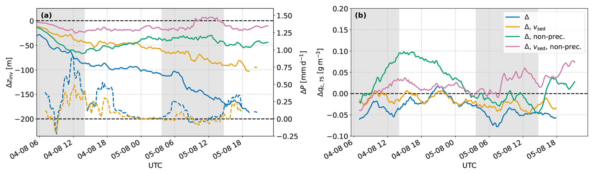
Figure 10Leg 16A difference plots for (a) the inversion height zinv (solid) as well as the surface precipitation rate P (dashed) and (b) the mean liquid water content in the top 75 m of the cloud qc,75. The blue line and the green line are the respective differences in the default precipitating and the default non-precipitating setup (cf. Fig. 8c for zinv). The orange line and the magenta line are the analogous respective differences, but with a halved sedimentation velocity in the drop_sed run. All lines apart from zinv were smoothed by a 3 h rolling mean. Shading as in Fig. 8.
For both non-precipitating cases (green, magenta), the only consistent decrease of Δzinv occurs during the initial period until the end of the first night. Analogously to the precipitating cases, this is weakened in the halved vsed case (magenta), which roughly stabilises afterwards, implying that both runs entrain similarly. At the end of the second night, the stable period is interrupted by a period of increased entrainment in the drop_sed run, that even briefly yields a higher net cloud-top height. Taking into account panel (b), the latter can be explained by a sudden excess in Δqc,75 during the second night, enabling stronger entrainment in the drop_sed run through evaporation. Furthermore, we can disentangle the other individual differences in the non-precipitating simulations. Interestingly, until the end of the first day, the simulation with the halved sedimentation speed ends up at lower amounts of liquid water near cloud-top (magenta below green) and also less LWP overall (cf. Fig. A4, dashed green vs. dashed orange). We can infer from this that the second-order liquid water reinforcement effect of the sedimenting droplets seems to be more powerful than the net loss of liquid water near cloud-top directly through sedimentation. In other words, even if vsed is higher and should deplete cloud-top more efficiently, the increased qc through the turbulent moisture redistribution can overcome this in the present thick case and yield a higher amount of liquid water near the top, strengthening the potential for evaporative cooling. These differences between green and magenta in panel (b) account for the steady rise of the green curve and the relatively stable magenta curve in panel (a). We can conclude that the initial decrease in Δzinv is evidently driven by vsed. After the initial stages, its major impact on precipitation continues, which drives the evolution in the drizzling simulations. In contrast, in the non-precipitating runs, it seems that after the initial period an unstable equilibrium is reached. This equilibrium appears to be largely unaffected by the magnitude of the sedimentation velocity in a direct way. It is, however, dependent on the base states of cloud liquid water near the top, which critically depend on the initial sedimentation speeds.
In this study, we investigated the effect of cloud droplet sedimentation on the initial deepening stage of the stratocumulus to cumulus transition in 10 cases of the MAGIC campaign. While we could confirm the previously known entrainment reduction (Bretherton et al., 2007; Wyant et al., 2007; Ackerman et al., 2009; Hill et al., 2009; de Lozar and Mellado, 2017; Pistor and Mellado, 2025) in the initial hours for all simulated legs, we found a different development on longer time scales. After the initial stage, the cases split into groups of precipitating, high-LWP legs (optically thick) versus non-precipitating, low-LWP legs (optically thin). The general evolution throughout the transect for either category in the drop_sed cases is illustrated in Fig. 11, with the inversion of the respective control case shown in grey dashed lines for comparison. It is assumed for simplicity that the thick (thin) legs always (never) precipitate.
The top panels summarise the evolution of the thick legs. In the initial stages after the activation of sedimentation, the cloud droplets sediment away from cloud-top, leading to reduced evaporative cooling and thus, reduced entrainment compared to control. Furthermore, this enhances drizzle formation, which is why the expected increase in LWP is turned into a net decrease. The drizzle production impedes turbulent circulations, which further works against boundary layer growth. In the intermediate to long-term stages, this behaviour continues. The amplified drizzle reduces LWP as well as turbulence and together with the sedimentation-evaporation feedback, the entrainment rate is lowered. The total longwave cooling is roughly unaffected, as the cloud is optically thick in every stage. The course of the thin legs in the bottom panels starts in a similar way. The sedimenting droplets naturally reduce entrainment, which in this case yields an increase in LWP, as no drizzle is present. This in turn increases the total longwave cooling rate, since it is not saturated in these legs. From here, the initial phase smoothly transitions to the long-term phase. The additional longwave cooling introduces stronger turbulent circulations that maintain and also amplify the moisture supply from the ocean surface. This enhances LWP production, which completes the feedback chain of LWP, longwave cooling and turbulence. The resulting amplification of TKE in the boundary layer counteracts the sedimentation flux from the top and is able to push liquid upwards, which increases the potential for evaporative cooling. Eventually, this yields increased entrainment and can even lead to a higher boundary layer compared to the control case. In our simulations, we observe that this cycle can persist for more than one day and is strongly dependent on the amount of liquid water in the cloud and the strength of drizzle production.
In Fig. 11, the separation from the initial phase to the long-term phase is denoted by a time scale t≫t0. It is tempting to quantify this time scale, which is terminated by the onset of the turbulence feedback mechanism. Deriving a universal value proves difficult, as we only have two thin cases to work with, one of which only starts to form a cloud late in the simulation. Furthermore, it is clear that this time scale is highly sensitive to various factors. The deciding factor here is the thickness of the cloud at the time of the activation of sedimentation, as not only the sedimentation velocity directly depends on it through droplet size, but also the increase in LWP and longwave cooling indirectly through the feedback mechanism. As evident from Fig. 9, the CCN concentration does not seem to interact with the initial decrease window, but suppressing precipitation does in the standard CCN scenario. Large-scale environmental conditions as e.g. the strength of the inversion (Sandu and Stevens, 2011) are likely to have an impact as well. With that in mind, we can extract the observed time scale for both thin legs. For Leg 11A, the initial decrease in zinv in the drop_sed run starts after the initial cloud formation at around 27 May, 06:00 and ends at 27 May, 12:00, yielding a 6 h period (e.g. Fig. 8d). Remarkably, this agrees pretty well with the spinup experiment of Leg 04A (cf. Fig. A2) starting at 21 October, 09:00 and roughly terminating between 21 October, 14:00 and 21 October, 15:00, yielding a 5 to 6 h period.
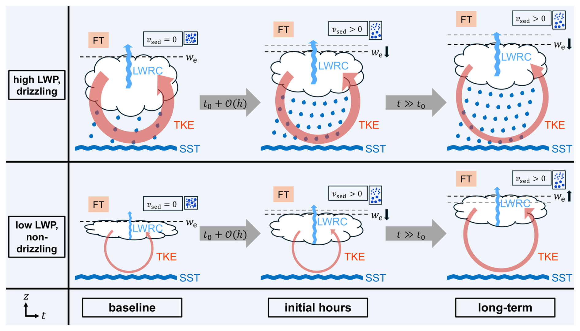
Figure 11Schematic to illustrate to impact of droplet sedimentation on the two different idealised cloud categories (top: optically thick and precipitating, bottom: optically thin and non-precipitating). Both show a similar initial effect regarding entrainment, but evolve structurally different afterwards. The first stage is the baseline state at time t0 before sedimentation is activated (indicated by vsed). The middle stage is the state in the initial hours and the last stage is the state after a longer period of time. The cloud thickness is a rough measure of the liquid water path (LWP), the light blue arrows indicate longwave radiative cooling (LWRC), while the red arrows indicate turbulent circulations (turbulent kinetic energy, TKE). The ocean surface is illustrated by blue waves (sea surface temperature, SST). Dashed lines represent the inversion height zinv under the dry free troposphere (FT), where entrainment occurs (marked by we), with the control inversion in grey for comparison, while the arrow thickness represents the strength of the respective quantity. Note that the light blue arrows are intentionally placed in the middle (bottom) of the cloud, if radiative cooling is saturated (unsaturated).
We identify this as the main difference from the simulations of Bretherton et al. (2007) and Pistor and Mellado (2025), both of which simulated active droplet sedimentation for 6 h. Their case from the first research flight (RF01) of the Second Dynamics and Chemistry of Marine Stratocumulus (DYCOMS-II) field campaign (Stevens et al., 2005) also belongs to the thin category with a LWP of around 40 g m−2. Note here that due to the specific setup, the DNS study of de Lozar and Mellado (2017) does not belong to the thin, but the thick category, even though they also took DYCOMS-II RF01 as a reference case (A. de Lozar, personal communication, 2026). As for Bretherton et al. (2007) and Pistor and Mellado (2025), we would expect an increase in entrainment in the presence of droplet sedimentation after the initial period based on our results. The observed reduction in both studies is not in contrast to our findings, if we take into account the identified initial phase of roughly 6 h, where entrainment is also reduced in our MAGIC simulations. So given that droplet sedimentation yields increased entrainment after a somewhat different time scale, it is likely not yet visible in the above relatively short simulations. This also serves as an explanation for the fact that Bretherton et al. (2007) and Pistor and Mellado (2025) found a negligible influence of longwave cooling. The short simulations are not able to capture the period, where the initial dominant impact of sedimentation is replaced by the turbulence feedback chain, with longwave cooling as a main contributor. Apart from that, there is also the third moment of the vertical wind, that structurally differs to our cases. While the profile in Pistor and Mellado (2025) turns negative below cloud-base, it is also mostly reduced in the presence of sedimentation. In the present cases the mean profile is always positive and increased (cf. Figs. 5, 7), pointing to a different organisation of up- and downdrafts. In contrast, we would not expect the LES result of Ackerman et al. (2009) to flip from the observed reduced to strengthened entrainment, if one would extend the simulation time. These simulations are not only precipitating, but also based on a different research flight (RF02) of DYCOMS-II with a LWP of around 100 g m−2, which is well in the saturated regime of longwave cooling.
Kurowski et al. (2025) also investigated the impact of cloud water sedimentation in a sensitivity experiment. While they did not directly study disabled sedimentation versus enabled sedimentation, they conducted a low sedimentation versus high sedimentation experiment in a precipitating case (i.e. comparable to our thick cases). They found that stronger sedimentation leads to a reduction in entrainment together with an increase in rain water, which aligns well with our findings in the optically thick category. We also observe increased precipitation rates as well as reduced boundary layer growth in our simulations, when comparing drop_sed to control (cf. Fig. 3a and c).
While cloud albedo susceptibility to aerosol perturbations is not the primary focus of this study, we would like to point out that the opposing changes in LWP between the two regimes lead to a mean decrease of −6.6 % in the pseudo-albedo when the cloud is saturated in the longwave, and a respective increase of 13.2 % when the longwave flux at cloud-top is not yet saturated. Even though this is only an overall mean, it underlines again that the effects in the optically thin cases are opposite, but of similar strength as in the optically thick cases. Thus, the mechanism suggested by Bretherton et al. (2007) regarding droplet sedimentation impacts on the LWP adjustment is still found to hold in more common thick clouds on time scales exceeding 6 h.
This time scale is consistent with the long time scales of around 10 h (Glassmeier et al., 2021) required for the full LWP adjustment to manifest as based on multiple LES runs of nocturnal stratocumuli. Also the processes identified here, namely longwave cooling and evaporative cooling, which impact entrainment and the response to droplet sedimentation, are consistent with identified leading processes driving these LWP equilibrium states in Hoffmann et al. (2020) and Glassmeier et al. (2021). The equilibrium states themselves are governed by large-scale drivers, such as low-troposphere divergence, surface fluxes, and the background aerosol concentration. The impact of droplet sedimentation may either accelerate or decelerate the rate at which a given equilibrium is approached. We do not quantify this here, as aerosol-cloud interactions and the LWP adjustment are not the focus of this study; instead, our primary objective is to examine the direction of cloud response induced by droplet sedimentation itself. Nonetheless, the impact on adjustment time scales is relevant to explore in future work, as characteristic time scales of changing external parameters and the time scale of LWP adjustments covary along the SCT. The impacts of which for quantifying the LWP adjustment are discussed in Feingold et al. (2025).
In addition, the diurnal cycle has been shown to drive distinct responses in LWP under day-time and night-time conditions (Smalley et al., 2024; Pugsley et al., 2025). In Sect. 4.1 we also found non-monotonic responses in entrainment speed to droplet sedimentation driven by shortwave heating during the day. This demonstrates the necessity for a more refined analysis of these processes with respect to the diurnal cycle. This was not done here, as our simulation set is too small to stratify for time of day in addition to their position along the SST gradient. While we can stratify for the spatial dimension (i.e. similar conditions in surface forcing), the legs do not coincide in time. For such analysis a much larger set of simulations (or multiple diurnal cycles) would be required.
Extending the discussion of high vs low LWP, we can address the importance of the two categories in reality. In doing so, we analyse one year of post-processed GOES 15 retrievals (Minnis et al., 2002, 2008, 2011) during the MAGIC period in the Northeast Pacific between [20° N, 35° N] and [117° W, 160° W]. We choose this region to include the full MAGIC transects between Los Angeles at [118.2° W, 34.1° N] and Honolulu at [157.9° W, 21.3° N]. Half-hourly day-time LWP data from 18:00 to 00:00 UTC are filtered for stratiform low clouds using the ISCCP thresholds of optical depth >3.6 and cloud-top pressure >680 hPa (Rossow and Schiffer, 1999). Separating them by the LWP threshold of 50 g m−2 as in Table 1, we obtain roughly 23 % in the thin category and 77 % in the thick category. This result is in good agreement with the corresponding LWP distribution for the Northeast Pacific, as well as with those observed in other subtropical stratocumulus decks (Murakami et al., 2021). This highlights the prevalence of the thick category, which also aligns with the present observation of eight thick and two thin cases. Thus, the majority of studies focusing on droplet sedimentation effects not only neglect longer time scales, but also concentrate on low-LWP cases, which constitute the minority of subtropical stratiform clouds (Bretherton et al., 2007; Schulz and Mellado, 2019; Igel, 2024; Pistor and Mellado, 2025).
Lastly, we can speculate about the impact of droplet sedimentation on the complete transition of stratocumulus to cumulus. The present 48 h runs are not enough to capture a full SCT. However, there are some thick legs, where the stratocumulus deck partially breaks up, indicated by its cloud fraction dropping below the 40 % threshold, and does not recover (cf. Table 1). As can be seen from Fig. A1, only for 07A, 13A, 14A and 17A this breakup occurs considerably before the end of the simulation. While all drop_sed runs consistently break up later, pointing at the enhanced sustainability of the cloud at low LWP, the specific timing is only marginally affected. The average delay of ≈40 km is strongly driven by the unstable winter case 07A, that shifts roughly 100 km, while the three summer legs vary below 25 km. Regarding the full deepening period of roughly 2000 km, we observe only little change. Extending this to a potential reformation of the stratocumulus deck during night-times, we can use Leg 17A as a proxy, where we also observe no considerable alterations in drop_sed compared to the control run (not shown). We cautiously interpret this as the aforementioned counteracting effects of enhanced precipitation and enhanced turbulence balancing each other, as soon as the cloud deck enters the low LWP regime. In fact, the amplified drizzle through sedimentation is not enough to lead to a runaway precipitation-driven SCT, as was observed by Yamaguchi et al. (2017). Thus, we conclude that the impact of cloud droplet sedimentation on the SCT in the thick legs regarding the qualitative initial deepening period is insubstantial and likely remains so in the later stages. There might be more substantial changes in the thin legs, as they are more strongly affected by the presented mechanism. However, this heavily depends on the onset of drizzle, as found for Leg 11A. So while these effects might be more potent, we still expect them to be minor overall, also due to the powerful influence of the large-scale conditions or the diurnal cycle.
This study addressed the impact of cloud droplet sedimentation in stratocumuli regarding longer time scales in the context of the stratocumulus to cumulus transition. We performed 48 h long large-eddy simulations in ICON along 10 selected MAGIC transects in the Northeast Pacific, conducting one control run and one with active cloud droplet sedimentation parametrisation for each case. We found the well-known entrainment reduction due to reduced evaporation in the initial hours of all cases, after which they show contrasting behaviour depending on their drizzle amount and LWP. The boundary layer in cases with high LWP (optically thick) and substantial precipitation continues to grow slower, reinforced by the stabilising effect of precipitation, while it rises faster in cases with low LWP (optically thin) and no precipitation. In the latter, the initial increase in LWP serves as the initiator for a feedback mechanism consisting of longwave radiative cooling, turbulent mixing and LWP. As the low-LWP clouds are not yet saturated in the longwave, the increase in LWP leads to an increase in net longwave cooling, which amplifies turbulent circulations. Those sustain the moisture supply for the cloud and further push liquid back to the entrainment zone, counteracting the direct depletion through the sedimenting droplets. As our simulations include two full days, we could demonstrate that high-LWP cases can transition to the other regime due to day-time thinning and experience the same mechanism, pointing towards a more robust and fundamental mechanism.
Sensitivity experiments disabling precipitation revealed that this effect is not solely a result of amplified drizzle in the drop_sed case. The LWP increase in the high-LWP cases does not have a strong impact on the already saturated longwave cooling, so that the feedback chain is suppressed and both the control run and the drop_sed run entrain similarly. Furthermore, we could show that the magnitude of the sedimentation velocity only drives the initial entrainment reduction, but has little impact on the longer time scales. In a third sensitivity experiment, we found that the background CCN concentration does not change the qualitative process chain either.
There are two important implications of our findings. Firstly, it is difficult to generalise results from a limited amount of cases, when studying the impact of a specific process. Regarding droplet sedimentation in subtropical stratocumuli, the majority of studies simulate one case with low LWP, while neglecting that this regime only represents the minority in reality. We acknowledge that the present 10 cases are not a large sample either, however, we could include synoptic variability and provide some statistics, that revealed clear regime differences. In general, it is important to incorporate various cases in the analysis in order to capture different mechanisms. Secondly, the common approach of studying the impact of droplet sedimentation in simulations of only a few hours obscures the long-term effect, which we have shown can be profoundly different from the initial hours.
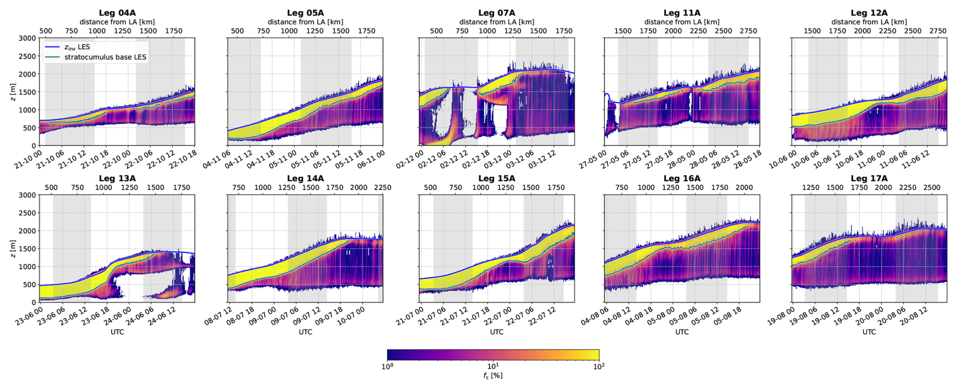
Figure A1Domain-averaged cloud fraction fc of the control runs for all legs. Colours and shading as in Fig. 1.
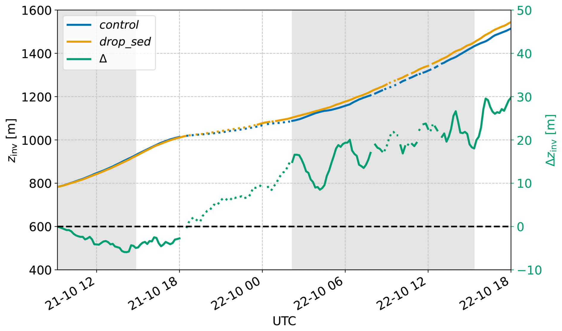
Figure A2Leg 04A inversion height zinv of the long spinup experiment, where droplet sedimentation is activated only after 15 h. Colours and shading as in Fig. 3. The dotted periods correspond to the stages where the mean cloud fraction is below 40 %.
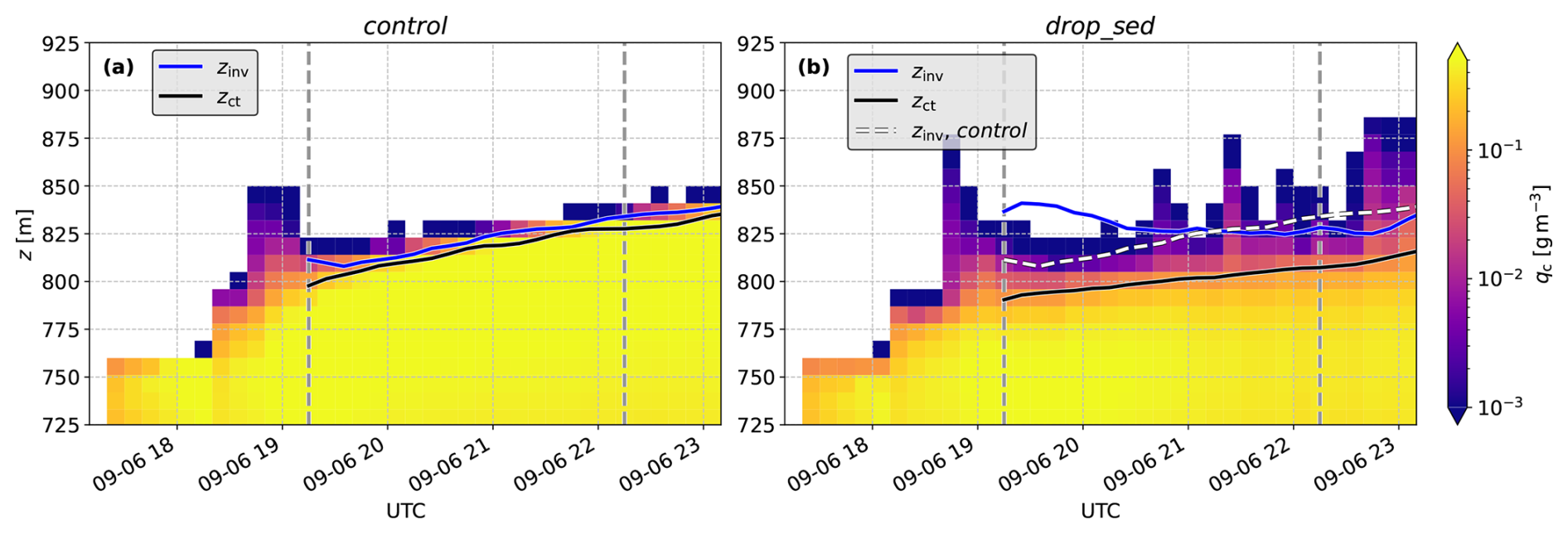
Figure A3Leg 12A liquid water content qc together with inversion height zinv and cloud-top height zct for the (a) control and (b) drop_sed simulation. The grey dashed lines mark the period analysed in Table 2. For clarity, the control inversion is shown as a white dashed line in panel (b).
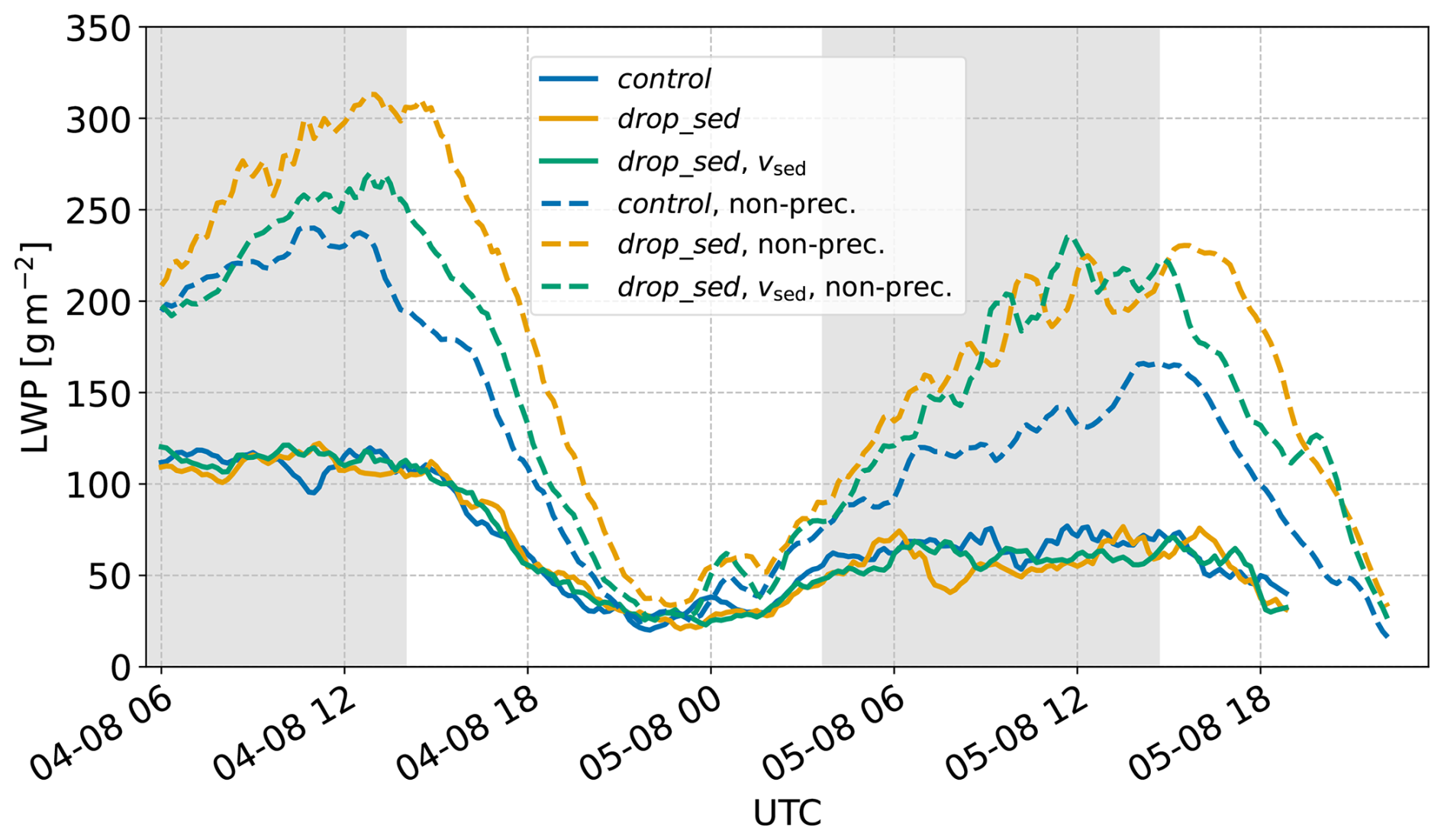
The ICON model is open source and can be downloaded from https://www.icon-model.org/ (last access: 29 June 2026). The specific version used in this study together with the input can be obtained from the authors upon request. The initial conditions and the large-scale forcings are based on the original forcings by McGibbon and Bretherton (2017) (https://github.com/GdR-DEPHY/DEPHY-SCM/tree/master/MAGIC, Roehrig et al., 2022) and were adapted for ICON. The data from the MAGIC campaign are available at https://www.arm.gov/ (last access: 30 October 2025), while the post-processed GOES 15 data are available from armarchive@arm.gov upon request. The data to create the plots are available from the Zenodo repository https://doi.org/10.5281/zenodo.21132428 (Schnelke, 2026).
MS conducted the simulations, analysed the data and wrote the initial draft. MA and MS designed the simulation setup. AP conceived the project and acquired the funding. All authors commented on the manuscript.
At least one of the (co-)authors is a member of the editorial board of Atmospheric Chemistry and Physics. The peer-review process was guided by an independent editor, and the authors also have no other competing interests to declare.
Publisher's note: Copernicus Publications remains neutral with regard to jurisdictional claims made in the text, published maps, institutional affiliations, or any other geographical representation in this paper. The authors bear the ultimate responsibility for providing appropriate place names. Views expressed in the text are those of the authors and do not necessarily reflect the views of the publisher.
MS would like to thank Axel Seifert for his expertise regarding the implementation of droplet sedimentation in ICON and Peter Blossey for his valuable assistance with the creation of the large-scale forcings. MS and AP appreciate support from the Hans Ertel Centre for Weather Research (Hans-Ertel-Zentrum für Wetterforschung; HErZ) funded by the Federal Ministry of Transport (grant number: 4823DWDP7). MA acknowledges support from HErZ and the German Weather Service (Deutscher Wetterdienst, DWD). This work used resources of the German Climate Computing Centre (Deutsches Klimarechenzentrum, DKRZ) granted by its Scientific Steering Committee (WLA) under project ID 1358.
This research has been supported by the Hans Ertel Centre for Weather Research funded by the Federal Ministry of Transport (grant number: 4823DWDP7), as well as the German Weather Service.
This open-access publication was funded by Goethe University Frankfurt.
This paper was edited by Guy Dagan and reviewed by two anonymous referees.
Ackerman, A. S., Kirkpatrick, M. P., Stevens, D. E., and Toon, O. B.: The Impact of Humidity above Stratiform Clouds on Indirect Aerosol Climate Forcing, Nature, 432, 1014–1017, https://doi.org/10.1038/nature03174, 2004. a, b
Ackerman, A. S., vanZanten, M. C., Stevens, B., Savic-Jovcic, V., Bretherton, C. S., Chlond, A., Golaz, J.-C., Jiang, H., Khairoutdinov, M., Krueger, S. K., Lewellen, D. C., Lock, A., Moeng, C.-H., Nakamura, K., Petters, M. D., Snider, J. R., Weinbrecht, S., and Zulauf, M.: Large-Eddy Simulations of a Drizzling, Stratocumulus-Topped Marine Boundary Layer, Mon. Weather Rev., 137, 1083–1110, https://doi.org/10.1175/2008MWR2582.1, 2009. a, b, c, d, e, f, g, h, i, j, k, l, m, n, o, p, q
Albrecht, B. A.: Aerosols, Cloud Microphysics, and Fractional Cloudiness, Science, 245, 1227–1230, https://doi.org/10.1126/science.245.4923.1227, 1989. a
Blahak, U.: New implementation of explicit hydrometeor sedimentation in the Seifert-Beheng 2-moment bulk microphysical scheme, https://www.cosmo-model.org/content/model/documentation/core/docu_sedi_twomom.pdf (last access: 1 September 2025), 2020. a
Blossey, P. N., Bretherton, C. S., and Wyant, M. C.: Subtropical Low Cloud Response to a Warmer Climate in a Superparameterized Climate Model. Part II: Column Modeling with a Cloud Resolving Model, J. Adv. Model. Earth Sy., 1, https://doi.org/10.3894/JAMES.2009.1.8, 2009. a, b, c
Blossey, P. N., Bretherton, C. S., and Mohrmann, J.: Simulating Observed Cloud Transitions in the Northeast Pacific during CSET, Mon. Weather Rev., https://doi.org/10.1175/MWR-D-20-0328.1, 2021. a, b
Bolt, S. and Omanovic, N.: Evaluation of semi-implicit and explicit sedimentation approaches in the two-moment cloud microphysics scheme of ICON, Geosci. Model Dev., 19, 595–619, https://doi.org/10.5194/gmd-19-595-2026, 2026. a
Brendecke, J., Dong, X., Xi, B., and Zheng, X.: Maritime Aerosol and CCN Profiles Derived From Ship-Based Measurements Over Eastern North Pacific During MAGIC, Earth Space Sci., 9, e2022EA002319, https://doi.org/10.1029/2022EA002319, 2022. a
Bretherton, C. S. and Wyant, M. C.: Moisture Transport, Lower-Tropospheric Stability, and Decoupling of Cloud-Topped Boundary Layers, J. Atmos. Sci., 54, 148–167, https://doi.org/10.1175/1520-0469(1997)054<0148:MTLTSA>2.0.CO;2, 1997. a, b, c
Bretherton, C. S., Blossey, P. N., and Uchida, J.: Cloud Droplet Sedimentation, Entrainment Efficiency, and Subtropical Stratocumulus Albedo, Geophys. Res. Lett., 34, 2006GL027648, https://doi.org/10.1029/2006GL027648, 2007. a, b, c, d, e, f, g, h, i, j, k, l, m, n, o, p, q
Bretherton, C. S., McCoy, I. L., Mohrmann, J., Wood, R., Ghate, V., Gettelman, A., Bardeen, C. G., Albrecht, B. A., and Zuidema, P.: Cloud, Aerosol, and Boundary Layer Structure across the Northeast Pacific Stratocumulus–Cumulus Transition as Observed during CSET, Mon. Weather Rev., 147, 2083–2103, https://doi.org/10.1175/MWR-D-18-0281.1, 2019. a
Christensen, M. W., Jones, W. K., and Stier, P.: Aerosols Enhance Cloud Lifetime and Brightness along the Stratus-to-Cumulus Transition, P. Natl. Acad. Sci. USA, 117, 17591–17598, https://doi.org/10.1073/pnas.1921231117, 2020. a
de Lozar, A. and Mellado, J. P.: Reduction of the Entrainment Velocity by Cloud Droplet Sedimentation in Stratocumulus, J. Atmos. Sci., 74, 751–765, https://doi.org/10.1175/JAS-D-16-0196.1, 2017. a, b, c, d, e, f, g
de Roode, S. R., Sandu, I., van der Dussen, J. J., Ackerman, A. S., Blossey, P., Jarecka, D., Lock, A., Siebesma, A. P., and Stevens, B.: Large-Eddy Simulations of EUCLIPSE–GASS Lagrangian Stratocumulus-to-Cumulus Transitions: Mean State, Turbulence, and Decoupling, J. Atmos. Sci., 73, 2485–2508, https://doi.org/10.1175/JAS-D-15-0215.1, 2016. a
Dipankar, A., Stevens, B., Heinze, R., Moseley, C., Zängl, G., Giorgetta, M., and Brdar, S.: Large eddy simulation using the general circulation model ICON, J. Adv. Model. Earth Sy., 7, 963–986, https://doi.org/10.1002/2015MS000431, 2015. a, b
Eastman, R. and Wood, R.: Factors Controlling Low-Cloud Evolution over the Eastern Subtropical Oceans: A Lagrangian Perspective Using the A-Train Satellites, J. Atmos. Sci., 73, 331–351, https://doi.org/10.1175/JAS-D-15-0193.1, 2016. a, b, c
Erfani, E., Blossey, P., Wood, R., Mohrmann, J., Doherty, S. J., Wyant, M., and O, K.-T.: Simulating Aerosol Lifecycle Impacts on the Subtropical Stratocumulus-to-Cumulus Transition Using Large-Eddy Simulations, J. Geophys. Res.-Atmos., 127, e2022JD037258, https://doi.org/10.1029/2022JD037258, 2022. a, b
Feingold, G., Cotton, W. R., Kreidenweis, S. M., and Davis, J. T.: The Impact of Giant Cloud Condensation Nuclei on Drizzle Formation in Stratocumulus: Implications for Cloud Radiative Properties, J. Atmos. Sci., 56, 4100–4117, https://doi.org/10.1175/1520-0469(1999)056<4100:TIOGCC>2.0.CO;2, 1999. a
Feingold, G., Koren, I., Yamaguchi, T., and Kazil, J.: On the reversibility of transitions between closed and open cellular convection, Atmos. Chem. Phys., 15, 7351–7367, https://doi.org/10.5194/acp-15-7351-2015, 2015. a
Feingold, G., Glassmeier, F., Zhang, J., and Hoffmann, F.: Opinion: Inferring process from snapshots of cloud systems, Atmos. Chem. Phys., 25, 10869–10885, https://doi.org/10.5194/acp-25-10869-2025, 2025. a
Glassmeier, F., Hoffmann, F., Johnson, J. S., Yamaguchi, T., Carslaw, K. S., and Feingold, G.: Aerosol-Cloud-Climate Cooling Overestimated by Ship-Track Data, Science, 371, 485–489, https://doi.org/10.1126/science.abd3980, 2021. a, b
Hill, A. A., Feingold, G., and Jiang, H.: The Influence of Entrainment and Mixing Assumption on Aerosol–Cloud Interactions in Marine Stratocumulus, J. Atmos. Sci., 66, 1450–1464, https://doi.org/10.1175/2008JAS2909.1, 2009. a, b, c, d
Hoffmann, F., Glassmeier, F., Yamaguchi, T., and Feingold, G.: Liquid Water Path Steady States in Stratocumulus: Insights from Process-Level Emulation and Mixed-Layer Theory, J. Atmos. Sci., 77, 2203–2215, https://doi.org/10.1175/JAS-D-19-0241.1, 2020. a
Hogan, R. and Bozzo, A.: A flexible and efficient radiation scheme for the ECMWF model: A flexible radiation scheme for the ECMWF model, J. Adv. Model. Earth Sy., 10, https://doi.org/10.1029/2018MS001364, 2018. a
Igel, A. L.: Processes Controlling the Entrainment and Liquid Water Response to Aerosol Perturbations in Nonprecipitating Stratocumulus Clouds, J. Atmos. Sci., 81, 1605–1616, https://doi.org/10.1175/JAS-D-23-0238.1, 2024. a, b
Keeler, E., Burk, K., and Kyrouac, J.: Balloon-Borne Sounding System (SONDEWNPN), 2012-10-01 to 2013-10-03, ARM Mobile Facility (MAG), Los Angeles, CA to Honolulu, HI – container ship Horizon Spirit; AMF2 (M1), Atmospheric Radiation Measurement (ARM) User Facility [data set], https://doi.org/10.5439/1595321, 2022. a
Klein, S. A. and Hartmann, D. L.: The Seasonal Cycle of Low Stratiform Clouds, J. Climate, 6, 1587–1606, https://doi.org/10.1175/1520-0442(1993)006<1587:TSCOLS>2.0.CO;2, 1993. a, b, c
Krueger, S. K., McLean, G. T., and Fu, Q.: Numerical Simulation of the Stratus-to-Cumulus Transition in the Subtropical Marine Boundary Layer. Part II: Boundary-Layer Circulation, J. Atmos. Sci., 52, 2851–2868, https://doi.org/10.1175/1520-0469(1995)052<2851:NSOTST>2.0.CO;2, 1995. a
Kurowski, M. J., Lebsock, M. D., and Smalley, K. M.: The diurnal susceptibility of subtropical clouds to aerosols, Atmos. Chem. Phys., 25, 15329–15342, https://doi.org/10.5194/acp-25-15329-2025, 2025. a, b, c, d, e
Lilly, D. K.: On the numerical simulation of buoyant convection, Tellus, 14, 148–172, https://doi.org/10.3402/tellusa.v14i2.9537, 1962. a
Lilly, D. K.: Models of cloud-topped mixed layers under a strong inversion, Q. J. Roy. Meteor. Soc., 94, 292–309, https://doi.org/10.1002/qj.49709440106, 1968. a
Louis, J.-F.: A parametric model of vertical eddy fluxes in the atmosphere, Bound.-Lay. Meteorol., 17, 187–202, https://doi.org/10.1007/BF00117978, 1979. a
McGibbon, J. and Bretherton, C. S.: Skill of ship-following large-eddy simulations in reproducing MAGIC observations across the northeast Pacific stratocumulus to cumulus transition region, J. Adv. Model. Earth Sy., 9, 810–831, https://doi.org/10.1002/2017MS000924, 2017. a, b, c, d, e, f, g, h, i, j
Meador, W. E. and Weaver, W. R.: Two-Stream Approximations to Radiative Transfer in Planetary Atmospheres: A Unified Description of Existing Methods and a New Improvement, J. Atmos. Sci., 37, 630–643, https://doi.org/10.1175/1520-0469(1980)037<0630:TSATRT>2.0.CO;2, 1980. a
Minnis, P., Nguyen, L., Doelling, D. R., Young, D. F., Miller, W. F., and Kratz, D. P.: Rapid Calibration of Operational and Research Meteorological Satellite Imagers. Part I: Evaluation of Research Satellite Visible Channels as References, J. Atmos. Ocean. Tech., 19, 1233–1249, https://doi.org/10.1175/1520-0426(2002)019<1233:RCOOAR>2.0.CO;2, 2002. a, b
Minnis, P., Nguyen, L., Palikonda, R., Heck, P. W., Spangenberg, D. A., Doelling, D. R., Ayers, J. K., Jr., W. L. S., Khaiyer, M. M., Trepte, Q. Z., Avey, L. A., Chang, F.-L., Yost, C. R., Chee, T. L., and Szedung, S.-M.: Near-real time cloud retrievals from operational and research meteorological satellites, in: Remote Sensing of Clouds and the Atmosphere XIII, edited by: Picard, R. H., Comeron, A., Schäfer, K., Amodeo, A., and van Weele, M., International Society for Optics and Photonics, SPIE, 7107, 710703, https://doi.org/10.1117/12.800344, 2008. a, b
Minnis, P., Sun-Mack, S., Young, D. F., Heck, P. W., Garber, D. P., Chen, Y., Spangenberg, D. A., Arduini, R. F., Trepte, Q. Z., Smith, W. L., Ayers, J. K., Gibson, S. C., Miller, W. F., Hong, G., Chakrapani, V., Takano, Y., Liou, K.-N., Xie, Y., and Yang, P.: CERES Edition-2 Cloud Property Retrievals Using TRMM VIRS and Terra and Aqua MODIS Data – Part I: Algorithms, IEEE T. Geosci. Remote S., 49, 4374–4400, https://doi.org/10.1109/TGRS.2011.2144601, 2011. a, b
Mohrmann, J., Bretherton, C. S., McCoy, I. L., McGibbon, J., Wood, R., Ghate, V., Albrecht, B., Sarkar, M., Zuidema, P., and Palikonda, R.: Lagrangian Evolution of the Northeast Pacific Marine Boundary Layer Structure and Cloud during CSET, Mon. Weather Rev., 147, 4681–4700, https://doi.org/10.1175/MWR-D-19-0053.1, 2019. a, b
Murakami, Y., Kummerow, C. D., and van den Heever, S. C.: On the Relation among Satellite-Observed Liquid Water Path, Cloud Droplet Number Concentration, and Cloud-Base Rain Rate and Its Implication to the Autoconversion Parameterization in Stratocumulus Clouds, J. Climate, 34, 8165–8180, https://doi.org/10.1175/JCLI-D-20-0473.1, 2021. a
Painemal, D., Minnis, P., and Nordeen, M.: Aerosol Variability, Synoptic-Scale Processes, and Their Link to the Cloud Microphysics over the Northeast Pacific during MAGIC, J. Geophys. Res.-Atmos., 120, 5122–5139, https://doi.org/10.1002/2015JD023175, 2015. a, b, c
Pistor, R. and Mellado, J. P.: Resolving Droplet Sedimentation Effects in Stratocumulus Clouds, J. Adv. Model. Earth Sy., 17, e2025MS004 966, https://doi.org/10.1029/2025MS004966, 2025. a, b, c, d, e, f, g, h, i, j, k, l, m
Pruppacher, H. R. and Klett, J. D.: Microphysics of Clouds and Precipitation, Springer Dordrecht, ISBN 9780792342113, 1997. a, b
Pugsley, G., Gryspeerdt, E., and Nair, V.: Cloud Fraction Response to Aerosol Driven by Nighttime Processes, P. Natl. Acad. Sci. USA, 122, e2509949122, https://doi.org/10.1073/pnas.2509949122, 2025. a
Roehrig, R., Vignon, E., Couvreux, F., Hourdin, F., Rio, C., and Lefebvre, M.-P.: GdR-DEPHY/DEPHY-SCM, Github [data set], https://github.com/GdR-DEPHY/DEPHY-SCM/tree/master (last access: 2 April 2024), 2022 a
Rossow, W. B. and Schiffer, R. A.: Advances in Understanding Clouds from ISCCP, B. Am. Meteorol. Soc., 80, 2261–2288, https://doi.org/10.1175/1520-0477(1999)080<2261:AIUCFI>2.0.CO;2, 1999. a
Sandu, I. and Stevens, B.: On the Factors Modulating the Stratocumulus to Cumulus Transitions, J. Atmos. Sci., 68, 1865–1881, https://doi.org/10.1175/2011JAS3614.1, 2011. a, b, c
Sandu, I., Stevens, B., and Pincus, R.: On the transitions in marine boundary layer cloudiness, Atmos. Chem. Phys., 10, 2377–2391, https://doi.org/10.5194/acp-10-2377-2010, 2010. a, b
Sarkar, M., Zuidema, P., Albrecht, B., Ghate, V., Jensen, J., Mohrmann, J., and Wood, R.: Observations Pertaining to Precipitation within the Northeast Pacific Stratocumulus-to-Cumulus Transition, Mon. Weather Rev., 148, 1251–1273, https://doi.org/10.1175/MWR-D-19-0235.1, 2019. a, b
Savic-Jovcic, V. and Stevens, B.: The Structure and Mesoscale Organization of Precipitating Stratocumulus, J. Atmos. Sci., 65, 1587–1605, https://doi.org/10.1175/2007JAS2456.1, 2008. a, b, c, d, e, f
Schnelke, M.: Dataset to reproduce the figures of“Opposing entrainment effects of cloud droplet sedimentation during the pre-breakup stage of the stratocumulus to cumulus transition”, Zenodo [data set], https://doi.org/10.5281/zenodo.21132428, 2026. a
Schulz, B. and Mellado, J. P.: Competing Effects of Droplet Sedimentation and Wind Shear on Entrainment in Stratocumulus, J. Adv. Model. Earth Sy., 11, 1830–1846, https://doi.org/10.1029/2019MS001617, 2019. a, b, c
Seifert, A. and Beheng, K. D.: A two-moment cloud microphysics parameterization for mixed-phase clouds. Part 1: Model description, Meteorol. Atmos. Phys., 92, 45–66, https://doi.org/10.1007/s00703-005-0112-4, 2006. a, b, c, d, e
Smagorinsky, J.: General Circulation Experiments with the Primitive Equations, Mon. Weather Rev., 91, 99–164, https://doi.org/10.1175/1520-0493(1963)091<0099:GCEWTP>2.3.CO;2, 1963. a
Smalley, K. M., Lebsock, M. D., and Eastman, R.: Diurnal Patterns in the Observed Cloud Liquid Water Path Response to Droplet Number Perturbations, Geophys. Res. Lett., 51, e2023GL107323, https://doi.org/10.1029/2023GL107323, 2024. a
Stephens, G. L.: Radiation Profiles in Extended Water Clouds. II: Parameterization Schemes, J. Atmos. Sci., 35, 2123–2132, https://doi.org/10.1175/1520-0469(1978)035<2123:RPIEWC>2.0.CO;2, 1978. a, b, c
Stephens, G. L.: The Parameterization of Radiation for Numerical Weather Prediction and Climate Models, Mon. Weather Rev., 112, 826–867, https://doi.org/10.1175/1520-0493(1984)112<0826:TPORFN>2.0.CO;2, 1984. a
Stevens, B., Cotton, W. R., Feingold, G., and Moeng, C.-H.: Large-Eddy Simulations of Strongly Precipitating, Shallow, Stratocumulus-Topped Boundary Layers, J. Atmos. Sci., 55, 3616–3638, https://doi.org/10.1175/1520-0469(1998)055<3616:LESOSP>2.0.CO;2, 1998. a, b, c, d, e
Stevens, B., Moeng, C.-H., Ackerman, A. S., Bretherton, C. S., Chlond, A., de Roode, S., Edwards, J., Golaz, J.-C., Jiang, H., Khairoutdinov, M., Kirkpatrick, M. P., Lewellen, D. C., Lock, A., Müller, F., Stevens, D. E., Whelan, E., and Zhu, P.: Evaluation of Large-Eddy Simulations via Observations of Nocturnal Marine Stratocumulus, Mon. Weather Rev., 133, 1443–1462, https://doi.org/10.1175/MWR2930.1, 2005. a
Turner, D. D., Vogelmann, A. M., Austin, R. T., Barnard, J. C., Cady-Pereira, K., Chiu, J. C., Clough, S. A., Flynn, C., Khaiyer, M. M., Liljegren, J., Johnson, K., Lin, B., Long, C., Marshak, A., Matrosov, S. Y., McFarlane, S. A., Miller, M., Min, Q., Minimis, P., O'Hirok, W., Wang, Z., and Wiscombe, W.: Thin Liquid Water Clouds: Their Importance and Our Challenge, B. Am. Meteorol. Soc., 88, 177–190, https://doi.org/10.1175/BAMS-88-2-177, 2007. a, b
Twomey, S.: The Influence of Pollution on the Shortwave Albedo of Clouds, J. Atmos. Sci., 34, 1149–1152, https://doi.org/10.1175/1520-0469(1977)034<1149:TIOPOT>2.0.CO;2, 1977. a
Twomey, S. A., Piepgrass, M., and Wolfe, T. L.: An assessment of the impact of pollution on global cloud albedo, Tellus B, 36B, 356–366, https://doi.org/10.1111/j.1600-0889.1984.tb00254.x, 1984. a
van der Dussen, J. J., de Roode, S. R., Ackerman, A. S., Blossey, P. N., Bretherton, C. S., Kurowski, M. J., Lock, A. P., Neggers, R. A. J., Sandu, I., and Siebesma, A. P.: The GASS/EUCLIPSE model intercomparison of the stratocumulus transition as observed during ASTEX: LES results, J. Adv. Model. Earth Sy., 5, 483–499, https://doi.org/10.1002/jame.20033, 2013. a, b
Williams, A. S. and Igel, A. L.: Cloud Top Radiative Cooling Rate Drives Non-Precipitating Stratiform Cloud Responses to Aerosol Concentration, Geophys. Res. Lett., 48, e2021GL094740, https://doi.org/10.1029/2021GL094740, 2021. a
Wood, R.: Stratocumulus Clouds, Mon. Weather Rev., 140, 2373–2423, https://doi.org/10.1175/MWR-D-11-00121.1, 2012. a, b, c
Wood, R., O, K.-T., Bretherton, C. S., Mohrmann, J., Albrecht, Bruce, A., Zuidema, P., Ghate, V., Schwartz, C., Eloranta, E., Glienke, S., Shaw, R. A., Fugal, J., and Minnis, P.: Ultraclean Layers and Optically Thin Clouds in the Stratocumulus-to-Cumulus Transition. Part I: Observations, J. Atmos. Sci., 75, 1631–1652, https://doi.org/10.1175/JAS-D-17-0213.1, 2018. a
Wyant, M. C., Bretherton, C. S., Rand, H. A., and Stevens, D. E.: Numerical Simulations and a Conceptual Model of the Stratocumulus to Trade Cumulus Transition, J. Atmos. Sci., 54, 168–192, https://doi.org/10.1175/1520-0469(1997)054<0168:NSAACM>2.0.CO;2, 1997. a, b, c
Wyant, M. C., Bretherton, C. S., Chlond, A., Griffin, B. M., Kitagawa, H., Lappen, C.-L., Larson, V. E., Lock, A., Park, S., de Roode, S. R., Uchida, J., Zhao, M., and Ackerman, A. S.: A Single-Column Model Intercomparison of a Heavily Drizzling Stratocumulus-Topped Boundary Layer, J. Geophys. Res.-Atmos., 112, https://doi.org/10.1029/2007JD008536, 2007. a, b, c, d, e
Yamaguchi, T., Feingold, G., and Kazil, J.: Stratocumulus to Cumulus Transition by Drizzle, J. Adv. Model. Earth Sy., 9, 2333–2349, https://doi.org/10.1002/2017MS001104, 2017. a, b, c, d
Zängl, G., Reinert, D., Rípodas, P., and Baldauf, M.: The ICON (ICOsahedral Non-hydrostatic) modelling framework of DWD and MPI-M: Description of the non-hydrostatic dynamical core, Q. J. Roy. Meteor. Soc., 141, 563–579, https://doi.org/10.1002/qj.2378, 2015. a
Zhang, D., Ermold, B., and Morris, V.: Ceilometer (CEIL), 2012-10-01 to 2013-09-26, ARM Mobile Facility (MAG), Los Angeles, CA to Honolulu, HI – container ship Horizon Spirit; AMF2 (M1), Atmospheric Radiation Measurement (ARM) User Facility [data set], https://doi.org/10.5439/1181954, 1996. a
Zheng, X., Klein, S. A., Ghate, V. P., Santos, S., McGibbon, J., Caldwell, P., Bogenschutz, P., Lin, W., and Cadeddu, M. P.: Assessment of Precipitating Marine Stratocumulus Clouds in the E3SMv1 Atmosphere Model: A Case Study from the ARM MAGIC Field Campaign, Mon. Weather Rev., 148, 3341–3359, https://doi.org/10.1175/MWR-D-19-0349.1, 2020. a
Zhou, X., Kollias, P., and Lewis, E. R.: Clouds, Precipitation, and Marine Boundary Layer Structure during the MAGIC Field Campaign, J. Climate, 28, 2420–2442, https://doi.org/10.1175/JCLI-D-14-00320.1, 2015. a, b, c, d