
the Creative Commons Attribution 4.0 License.
the Creative Commons Attribution 4.0 License.
 | 08 Jul 2026
Improved constraints on ammonia emissions and deposition from co-assimilating NH3 and NO2 satellite observations over the Netherlands
Enrico Dammers
Arjo Segers
Mark W. Shephard
Pierre Coheur
Lieven Clarisse
Martin Van Damme
Henk Eskes
Roy Wichink Kruit
Shelley van der Graaf
Martijn Schaap
Ammonia (NH3) and nitrogen dioxide (NO2) are key components of reactive nitrogen, strongly affecting air quality and ecosystem health. However, long-term constraints on ammonia emissions and deposition remain uncertain due to sparse in situ measurements and limitations of individual satellite products. We jointly assimilate five years (2018–2022) of NH3 and NO2 satellite observations over the Netherlands to improve constraints on reactive nitrogen concentrations, emissions, and deposition. NH3 retrievals from the Infrared Atmospheric Sounding Interferometer (IASI) and the Cross-Track Infrared Sounder (CrIS) are combined with NO2 observations from the TROPOspheric Monitoring Instrument (TROPOMI) within the LOTOS-EUROS chemical transport model using a Local Ensemble Transform Kalman Filter. The co-assimilation produces coherent year-to-year adjustments in modeled NH3 concentration, emission, and deposition fields. Validation against measurements from the Dutch National Air Quality Monitoring Network (LML) shows reduced biases, clearer diurnal cycles, and improved correlations. Sensitivity experiments demonstrate that including TROPOMI NO2 alongside IASI and CrIS NH3 yields the lowest NH3 surface bias vs. LML, highlighting the added value of coupling chemically related satellite observations. Comparisons with monthly Measurements of Ammonia in Nature (MAN) observations showed improved correlations but persistent spatial biases due to representativeness differences, while MAN sensors co-located with LML stations exhibited consistent improvements. These results demonstrate that co-assimilating complementary satellite observations can substantially improve constraints on ammonia emissions and deposition, with direct relevance for air-quality assessment and nitrogen policy applications.
- Article
(26468 KB) - Full-text XML
- BibTeX
- EndNote


Ammonia (NH3) and nitrogen dioxide (NO2) are key reactive nitrogen species that play central roles in atmospheric chemistry and air quality. Through dry and wet deposition, these gases contribute substantially to the transfer of reactive nitrogen to the Earth's surface, where they influence both terrestrial and aquatic ecosystems. Although reactive nitrogen is essential for plant growth and ecosystem functioning, excessive deposition can cause environmental degradation, including soil acidification, eutrophication, and biodiversity loss (Galloway et al., 2008; Sutton et al., 2011).
NH3 is the most abundant alkaline gas in the atmosphere, primarily emitted from agricultural activities such as livestock farming and fertilizer application (Erisman et al., 2011; Galloway et al., 2008). In agriculture, NH3 is released through the decomposition of animal waste and the volatilization from nitrogen-rich fertilizers applied to soils (Erisman et al., 2008, 2011; Sutton et al., 2011; Paulot et al., 2014). This gas plays a vital role in the formation of secondary inorganic aerosols (SIAs) by reacting with acidic compounds such as sulfuric and nitric acids to form ammonium sulfate and ammonium nitrate (Erisman et al., 2011). SIAs contribute to fine particulate matter (PM2.5), which affects atmospheric visibility and poses significant health risks, including respiratory and cardiovascular diseases (Pope and Dockery, 2006; Pope et al., 2009).
NO2 in the atmosphere originates primarily from nitric oxide (NO), which is emitted during fossil fuel combustion in vehicles, power plants, and industrial processes and rapidly oxidized in air. Together, NO and NO2 form the NOx family, a key precursor to tropospheric ozone and nitrate aerosols (Crutzen, 1979; Ojeda-Castillo et al., 2025; Zara et al., 2021). NO2 participates in photochemical reactions leading to the formation of ozone and particulate nitrates, contributing to air pollution and smog formation (Zhang et al., 2011). In addition, NO2 indirectly influences the atmospheric lifetime of NH3 by modulating the production of nitric acid (HNO3): increased oxidation of NO2 enhances HNO3 formation, which in turn promotes the partitioning of NH3 into ammonium nitrate. Elevated levels of NO2 and its reaction products are associated with respiratory problems such as asthma and decreased lung function, and contribute to environmental degradation through acid deposition and nutrient imbalances in ecosystems (Eum et al., 2022; Jonson et al., 2017; Liu et al., 2021).
Understanding the spatial and temporal distributions of NH3 and NO2 is essential for accurate atmospheric modeling and the development of effective emissions control strategies and regulations. However, the reactive nature and short atmospheric lifetimes of NH3 and NO2 pose significant challenges to monitoring and modeling of these species. Emissions inventories derived from bottom-up approaches often have large uncertainties associated with them, particularly in the case of NH3 where these uncertainties can be greater than 100 % for some emissions sectors (Kuenen et al., 2022). Ground-based measurement networks provide high-accuracy observations but differ greatly in spatial density; NO2 is routinely monitored at hundreds of sites across Europe, whereas NH3 is measured at far fewer locations, resulting in much sparser spatial coverage and limited temporal resolution. Moreover, these networks generally measure surface concentrations and do not provide full atmospheric column information. Space-based observations from instruments such as IASI on the MetOp series, CrIS on the Suomi-NPP and NOAA-20/21 platforms, and TROPOMI on Sentinel-5 Precursor offer broader spatial coverage, but with limited temporal sampling due to discrete overpass times. Satellite measurements of this type can be subject to errors resulting from, for example, instrumental noise, retrieval biases, and residual cloud cover.
Inverse modeling methods present a powerful approach to overcome these limitations by integrating observational data into chemical transport models to yield optimized estimates of atmospheric constituents. By assimilating large numbers of NH3 and NO2 measurements, it is possible to improve the accuracy of simulated concentrations, diurnal cycles, and associated emission and deposition fields. Assimilating NO2 observations in particular helps to better constrain the NOx budget, which in turn reduces uncertainties in the formation and loss of nitric acid (HNO3) and thus indirectly constrains the NH3 fields through their chemical coupling. Through such an approach, air quality predictions can be improved and policy-relevant insights can be gained for mitigating the impacts of reactive nitrogen on ecosystems and human health.
In this paper, we perform a co-assimilation of measurements of NH3 from IASI, CrIS and NO2 from TROPOMI in the LOTOS-EUROS local ensemble transform Kalman filter (LETKF) over a model domain encompassing the Netherlands and adjacent parts of northwestern Germany. This is a particularly relevant region for studying atmospheric NH3, as it forms a major reactive nitrogen hot-spot in Europe due to intensive agriculture, especially livestock production and fertilizer use. At the same time, accurate quantification of NH3 is particularly important for the Netherlands given the ongoing nitrogen crisis and the associated pressures of nitrogen deposition on sensitive ecosystems. Including the neighboring German source regions is also necessary because NH3 and secondary inorganic nitrogen are influenced by cross-border transport, such that concentrations and deposition over the Netherlands cannot be interpreted from domestic emissions alone. We evaluate resulting optimized emissions and deposition fields, with a focus on NH3, and we compare the results against independent observations from ground-based measurement networks.
2.1 The LOTOS-EUROS model
In this study, we utilized the LOTOS-EUROS (LOng Term Ozone Simulation-EURopean Operational Smog) v2.2.009 chemical transport model to simulate atmospheric concentrations over the study region (Manders et al., 2017). LOTOS-EUROS is a three-dimensional Eulerian model designed for regional air quality assessments and operational forecasting in Europe. It effectively simulates the dispersion, chemical transformation, and deposition of atmospheric pollutants, including gases and aerosols. LOTOS-EUROS is part of the Copernicus Atmospheric Monitoring Service (CAMS) European air quality ensemble (Colette et al., 2025). This service provides forecasts for the main air pollutants using an ensemble of state-of-the-science CTMs. Within CAMS, LOTOS-EUROS is regularly validated against in-situ observations and TROPOMI satellite data, as well as evaluation against the other ensemble members (Peuch et al., 2022; Colette et al., 2025). LOTOS-EUROS also has participated in numerous model inter-comparisons, typically showing a strong performance (Bessagnet et al., 2016; Colette et al., 2017; Vivanco et al., 2017).
The model incorporates detailed representations of atmospheric processes such as advection, diffusion, bi-directional fluxes, and chemical reactions. It uses the Carbon Bond Mechanism IV (CBM-IV) for gas-phase chemistry, which includes a comprehensive set of reactions relevant to ozone formation and other photochemical oxidants. Aerosol dynamics are modeled using size-resolved modules that account for primary emissions, secondary formation, and processes like coagulation and deposition.
Model outputs, including concentrations of key pollutants such as NH3, NO2, ozone (O3), and particulate matter (PM10 and PM2.5), are regularly validated against observational data from the Dutch LML air quality monitoring network, measurements from the German environmental agency (the Umweltbundesamt; UBA) and the EBAS network throughout the European Union. The NH3, NO2 and particulate matter components from the model are also frequently validated against the EMEP model and other models within the CAMS model ensemble (Schaap et al., 2008; Manders et al., 2017; Tsyro et al., 2022).
2.1.1 The Local ensemble transform Kalman filter
The Ensemble Kalman filter (EnKF; Evensen, 2003) is a sequential data assimilation method in which uncertainties in the model state are represented by an ensemble of simulations, which is updated using observations. In this study, we use the Local Ensemble Transform Kalman Filter (LETKF), a localized formulation of the EnKF that updates the model state by combining the ensemble forecast with observations within a defined spatial neighborhood. The LOTOS-EUROS LETKF v3.0.7 applied here has previously been used in studies of particulate matter (Lopez-Restrepo et al., 2020), NO2 (Timmermans et al., 2019), and NH3 (Van Der Graaf et al., 2022). The formulation is described in Hunt et al. (2007), and the implementation used here follows Shin et al. (2016). Compared with the standard Ensemble Kalman Filter, the LETKF is more computationally efficient and performs the analysis on a per-grid-cell basis using only nearby observations, which are determined using a specified spatial localization length (discussed in further detail in Sect. 2.1.2).
In the present application, the LETKF uses an augmented state vector,
where c denotes the three-dimensional trace-gas concentration fields and β denotes one or more two-dimensional emission perturbation fields for the optimized species. The primary objective of the filter is to estimate β, which defines multiplicative per-grid-cell scaling factors applied to the prior emissions. The perturbed emissions are computed as
where Ebase is the prior emission field. This clipping ensures that the updated emissions remain non-negative and prevents non-physical emission sinks. The concentration field c is included in the augmented state because it provides the dynamical link between the emission perturbations and the observations. During the forecast step, the model propagates the concentration fields forward using emissions modified by the current β values, so that free-running simulations, or simulations in regions without recently assimilated observations, remain influenced by earlier analysis updates.
The temporal variability in the emissions is specified in the assimilation through the temporal correlation length τ (set to 3 d for NH3 based on Van Der Graaf et al., 2022, and 1 d for NO2), with the temporal correlation coefficient α defined as Lopez-Restrepo et al. (2020), Van Der Graaf et al. (2022):
where tk and tk−1 are successive hourly analysis times. This formulation ensures that, in the absence of new observations for an extended period, the influence of past updates diminishes and the system progressively returns toward the a priori emission state. The LETKF analysis is applied at hourly analysis times throughout the simulation period. At each analysis time tk, only the emission state corresponding to the current time step is updated; emissions from previous time steps are not retrospectively adjusted. The temporal correlation coefficient αk in Eq. (3) therefore does not define a multi-time assimilation window, but instead controls the persistence of emission adjustments between successive hourly analysis times.
In the main co-assimilation configuration used in this study, species-specific emission perturbation factors are optimized simultaneously for both NH3 and NO2. As a result, assimilated NO2 observations constrain the NOx emission field directly rather than allowing their signal to be attributed to NH3 emissions alone. The uncertainty in this system is represented by an ensemble of N members. In this study, N=12 was used following Van Der Graaf et al. (2022), who applied the same LOTOS-EUROS LETKF framework. This relatively modest ensemble size is feasible here because the analysis is strongly localized in space and the short atmospheric lifetimes of NH3 and NO2 lead to comparatively compact, local covariance structures. For the initialization of the ensemble, the emission perturbation factors are sampled from a normal distribution with a mean of 1.0 and a standard deviation of 0.5, corresponding to 50 % uncertainty around the prior emissions. The resulting emissions are then constrained through Eq. (2), such that perturbation factors that would otherwise produce negative emissions instead yield zero.
The LETKF operates in two sequential steps, the forecast and the analysis. In the forecast step, the state vector ensemble is propagated forward in time using the model dynamics, where represents the ith forecast ensemble member. Each analyzed ensemble member at time tk−1 is propagated forward to tk according to Van Der Graaf et al. (2022):
where the model operator Mk−1 describes the forward model simulation from tk−1 to tk, including the application of the emission perturbation factors to the prior emissions and the persistence of β between successive analysis times through the temporal correlation coefficient αk. Here, denotes the ith analyzed ensemble member at time tk−1. Once the ensemble has been propagated forward in time, the ensemble mean and forecast error covariance Pf are calculated as
When new observations yobs are available, the analysis ensemble Xa is obtained by updating each ensemble member according to Van Der Graaf et al. (2022):
Here, denotes the model-simulated equivalent of the satellite retrieval, H is the linearized observation operator, R is the observation error covariance matrix, and Pa is the analysis error covariance, which is computed from Shin et al. (2016):
The simulated satellite observations are computed following the averaging kernel formalism of Rodgers (2000) and Rodgers and Connor (2003). First, the model state is interpolated to the retrieval grid using the gridding operator G:
To ensure that the comparison with the satellite product is made at the same effective vertical resolution as the retrieval, the averaging kernel A is applied:
where xa is the a priori profile used in the retrieval. In the linear approximation, the observation operator becomes:
The observations are assumed to satisfy
with R taken from the retrieval error covariance matrices of the satellite data products and represents both measurement and representativeness errors (Van Der Graaf et al., 2022). Once the update is complete, the analyzed ensemble Xa becomes the initial condition for the next forecast step.
2.1.2 Spatial localization
To ensure computational efficiency and avoid spurious correlations, the LETKF applies spatial and temporal localization in a per-grid-cell approach following Shin et al. (2016). In contrast to approaches that apply covariance localization directly to the background error covariance matrix, the LETKF implementation used here applies localization in observation space by selecting and weighting nearby observations for each local analysis. As a result, the localization length in this framework should be interpreted as application-specific and is not expected to match the much larger values used in numerical weather prediction studies such as Shin et al. (2016), where the analyzed variables exhibit broader synoptic-scale spatial correlations. The temporal localization was described in the previous section, and is applied using Eq. (3). For the spatial localization, the simulated observations are first computed for all ensemble members, and then for the given grid cell to be analyzed, all observations (both simulated and real) within 3.5ρ distance are gathered, with ρ being the specified localization length (in units of km). The analysis is then performed using the collected observations, with the contribution of each observation to the local analysis decreasing smoothly with distance from the analyzed grid cell. In the present implementation, this distance weighting is represented using a Gaussian decay function:
where Δd is the distance (in km) between the observation and the model grid point. Thus, observations closest to the analyzed grid cell have the largest influence, while the contribution of more distant observations decreases smoothly with distance. This is consistent with the localized observation-space LETKF framework described by Shin et al. (2016), although the functional form shown here corresponds to the implementation used in the present study. In this study, the spatial correlation lengths are chosen to be consistent with the horizontal representativeness of the corresponding satellite retrievals and are therefore guided by the mean footprint sizes. This also reflects the relatively local emission-concentration relationships of short-lived reactive gases such as NH3 and NO2. Using a localization length much larger than the footprint would allow a single observation to influence the analysis over spatial scales that are not resolved by the measurement, potentially producing spurious long-range increments and unrealistically smooth updates. To ensure spatial consistency between the retrieval resolution and its influence in the LETKF, we use ρ=15 km for CrIS and IASI NH3 and a smaller ρ=5 km for TROPOMI NO2, reflecting the higher spatial resolution of the latter.
2.1.3 Model configuration
In this section, a short summary of the most important model inputs and configuration parameters are provided. For a more detailed description of the LOTOS-EUROS model we direct the reader to Manders et al. (2017). The LETKF v3.0.7 is coupled to version 2.2.009 of the LOTOS-EUROS model. An initial long simulation covering the period of 2018–2022 was performed on a domain that covers the majority of Europe (15° W–35° E; 35–70° N) with a resolution of approximately 25 km×25 km, and the output from this run was utilized as boundary conditions for the assimilation run which was performed on a domain covering most of North-western Europe (2–16° E; 47–56° N) with a resolution of 7 km×7 km. The model is driven by meteorological fields obtained from the ECMWF short-term forecast model at a 3-hourly temporal resolution which is then interpolated to an hourly frequency within the model. The simulations were conducted using 12 vertical levels, extending from the ground to about 10 km above the earth's surface, matching the vertical layer structure of the ECMWF meteorology dataset.
The base emission dataset used in the model simulations combines the European-scale CAMS-REG-v5.1 inventory (Kuenen et al., 2022) with higher-resolution national inventories for the Netherlands (Emissieregistratie; ER) and Germany (Gridding Emission Tool for ArcGIS; GRETA). This combined CAMS GRETA-ER emissions dataset was developed within the National Kennisprogramma Stikstof (NKS) funded by the Dutch Ministry of Agriculture, Fisheries, Food Security and Nature (LVVN). The base emission dataset was compiled using the corresponding inventory year where available; for years after 2019, the 2019 emission totals were used as the baseline because 2019 was the most recent year available in the harmonized CAMS-GrETa-ER emissions dataset, and these emissions were then adjusted dynamically according to meteorological conditions. As a result, year-to-year variations in the base emissions remain relatively small and primarily reflect meteorological influences rather than structural changes in activity or policy. Temporally, the emissions are distributed using hourly time factors specific to aggregated source categories. For agricultural NH3 emissions, a meteorologically dependent parameterization is applied that accounts for weather-driven shifts in fertilizer application timing, following the approach of Ge et al. (2020). Emissions are also vertically distributed according to sector-specific release heights, which is particularly relevant for industrial and power-generation sources where average stack heights determine the initial plume elevation.
The model output for all major nitrogen species consists of simulated concentrations (surface, and all vertical layers) and wet and dry deposition, as well as concentrations matched at the footprints of all satellite products (i.e. IASI, CrIS, TROPOMI). To match the model with the satellite footprints, and for the ingestion of these observations in the LETKF, the CAMS Satellite Operator (CSO) is used. CSO (https://ci.tno.nl/gitlab/cams/cso, last access: 6 July 2026) is an open-access tool developed at the Netherlands Organisation for Applied Scientific Research (TNO) and implemented to facilitate fast intercomparisons between modelled and satellite concentrations. The tool consists of two entities: a pre-processor to download, select, and convert satellite observations into a common format, accompanied by post-processing tools to aggregate and visualize the data; and a source code that can be used within regional air quality modelling and assimilation systems such as LOTOS-EUROS. The CSO module is able to read the files created by the pre-processor, simulate satellite observations using model variables, and apply observational operators where applicable.
2.2 Satellite datasets
In the LETKF configuration used in this study, the assimilated satellite observations consist of NH3 total columns from IASI and CrIS, and NO2 tropospheric vertical column densities from TROPOMI.
2.2.1 IASI NH3
The IASI instruments onboard the MetOp-A, -B, and -C satellites are in sun-synchronous orbits, with Equator crossing times at approximately 09:30 and 21:30 LT (Clerbaux et al., 2009). Although the three platforms fly in the same local-time orbit, they are phased along that orbit and therefore do not acquire measurements simultaneously over the same ground location; the temporal separation between the platforms is on the order of 45 min. The data products of IASI-A, -B, and -C span the periods October 2007–October 2021 (IASI-A), March 2013 onward (IASI-B), and September 2019 onward (IASI-C), with the latter two instruments still operational. Each of the three IASI instruments has an observational swath width exceeding 2000 km, with a pixel footprint of approximately 12 km in diameter at nadir, increasing to around at the swath edges. In this study, we utilize the most recent IASI product, the Artificial Neural Network for IASI (ANNI)v4 (Clarisse et al., 2023), which is an updated version of the earlier IASI-NNv2 and LUT products (Van Damme et al., 2014, 2017).
Similar to its predecessors, the IASI-ANNIv4 retrieval involves two steps. First, the hyperspectral range index (HRI) is calculated to characterize the NH3 signal strength in each spectrum (Van Damme et al., 2017; Clarisse et al., 2023). The second step utilizes a neural network trained on a large dataset of modeled data, which links the HRI to the NH3 total column. The primary improvement in this version is the addition of a column averaging kernel to facilitate comparisons with in-situ and model data, enabling the effects of the a-priori profile shape to be considered. Earlier ANNI NH3 products were evaluated in previous studies by Dammers et al. (2016), Guo et al. (2021), Kutzner et al. (2021), Herrera et al. (2022), including against ground-based FTIR observations from the Network for the Detection of Atmospheric Composition Change (NDACC). The validation of IASI NH3 against NDACC measurements by Dammers et al. (2016) showed on average favorable correlations (R=0.80), with a mean low bias on the order of 35 %.
In the current study, we apply the recommended data quality filters, namely, with the pre-filter and post-filter set to 1, and only observations with a cloud_fraction <25 % are used.
2.2.2 CrIS NH3
The CrIS-1 instrument on the Suomi-NPP and CrIS-2 on NOAA-20 were launched in October 2011 and November 2017, respectively, with CrIS-Fast Physical Retrieval (CFPR) NH3 data products starting in May 2012 and March 2019. Both instruments are in sun-synchronous orbits, providing global coverage twice daily at around 13:30 and 01:30 local solar time, with overpasses within 45 min of each other. They offer observations with circular pixel footprints of approximately 14 km at nadir over a 2200 km wide swath. This study utilizes the CFPR NH3 product version 1.6.4 (Shephard and Cady-Pereira, 2015; Shephard et al., 2020). The CFPR method involves a physical retrieval based on the Rodgers (2000) optimal estimation method combined with a fast optimal spectral sampling forward model (Moncet et al., 2008), minimizing the residual between measured and simulated spectra. The excellent signal-to-noise ratio (∼1600) of the CrIS instrument in the ammonia spectral region enables detection sensitivities of approximately 0.5 ppbv near the surface, or 3.5×10¹⁵ for total columns, under typical atmospheric conditions (∼50 % detection rate). Under highly favorable infrared remote sensing conditions (e.g. strong thermal contrast) the detection limit can improve to about 0.2 ppbv, corresponding to a ∼10 % detection rate (Shephard et al., 2025). Since the last major validation study by Dammers et al. (2017), the product has undergone several iterations, including the addition of a cloud flag based on VIIRS data, non-detects, and a quality flag (White et al., 2023). The validation study by Dammers et al. (2017) reported a good correlation between FTIR and satellite observations (R≈0.8) with a slight high bias (slope=1.02). For higher column concentrations, CrIS observations showed a small positive difference with the ground-based FTIR measurements around 25 %–50 %, while for lower concentrations, the bias increased to 2.5×10¹⁵ with a standard deviation of around 50 %–100 %. This study only includes observations with a quality_flag of ≥3, thereby excluding failed or lower-confidence retrievals, and with a cloud_flag equal to 0 (clear-sky scenes). Only daytime observations are assimilated. It should be noted that the CrIS-1 instrument suffered a failure of its mid-wave IR (MWIR) band from 26 March to 24 June 2019, leading to a data gap in this period (Iturbide-Sanchez et al., 2022).
2.2.3 TROPOMI NO2
The TROPOMI instrument, aboard the Sentinel-5 Precursor (S5P) polar-orbiting satellite, is a nadir-viewing spectrometer designed for atmospheric observations. It crosses the equator at approximately 13:30 LT. The instrument measures radiation across the ultraviolet, visible, and infrared spectral ranges, enabling the monitoring of atmospheric trace gases and aerosols (Veefkind et al., 2012). TROPOMI has a swath width of approximately 2600 km, and the NO2 product has a nadir spatial resolution of 7.2 km in the along-track direction and 3.6 km in the across-track direction, improving to 5.6 km×3.6 km after 6 August 2019 (van Geffen et al., 2022). The retrieval of NO2 columns follows a three-step process. First, the NO2 slant column density is calculated from the L1b spectra recorded by TROPOMI using a DOAS fitting algorithm. This slant column is then separated into stratospheric and tropospheric components through data assimilation using the TM5-MP model, which operates at a horizontal resolution of 1°×1° (Williams et al., 2017). Finally, slant column densities are converted to vertical column densities (VCD) by applying total and altitude-dependent air mass factors (AMFs). These AMFs are influenced by several factors, including NO2 vertical profiles obtained from TM5-MP, the satellite's viewing geometry, surface albedo, surface pressure, and characteristics of clouds and aerosols. Further details on the retrieval process can be found in van Geffen et al. (2022) and in the algorithm theoretical baseline document (van Geffen et al., 2024).
Routine validation of TROPOMI NO2 measurements against ground-based MAX-DOAS observations from 29 stations has revealed a mean bias of −28 %, increasing to −40 % in regions with heavy pollution (Lambert et al., 2024). This bias largely stems from the TM5-MP vertical profiles, which inadequately resolve high-concentration hot-spots and show deviations in the profile shape, particularly near the surface (Chan et al., 2020; Verhoelst et al., 2021). To address these discrepancies, the a-priori vertical profile can be updated using one derived from a higher-resolution air quality model, which has been shown to partially mitigate biases (Griffin et al., 2019; Zhao et al., 2020; Judd et al., 2020; Douros et al., 2023). This correction process employs TROPOMI averaging kernels and is described in detail in the TROPOMI NO2 Product User Manual (Eskes et al., 2024).
In this study, we used the VCDs from the reprocessed TROPOMI NO2 version 2.4.0 dataset. To ensure data reliability, observations with a quality assurance value below 0.75 were excluded. This threshold effectively eliminates pixels with cloud radiance fractions exceeding 0.5, thereby reducing the impact of uncertain retrievals (van Geffen et al., 2022).
2.3 Ground-based in-situ measurements
2.3.1 The LML network
The Dutch National Air Quality Monitoring Network, known as the “Landelijk Meetnet Luchtkwaliteit” (LML) (Elskamp, 1989; Elzakker and Buijsman, 1999), is a comprehensive ground-based measurement network designed to monitor air quality across the Netherlands. Operated by Rijksinstituut voor Volksgezondheid en Milieu (RIVM), the LML network consists of a large number of monitoring stations distributed across urban, suburban, and rural areas. These stations continuously collect data on various air pollutants, including PM10, PM2.5, NO2, NH3, O3, sulfur dioxide (SO2), carbon monoxide (CO), and volatile organic compounds (VOCs).
The network provides real-time data, which is crucial for assessing the air quality in different regions and understanding the impact of pollution on public health and the environment. LML stations employ state-of-the-art sensors and analytical techniques to ensure high data accuracy and consistency, enabling authorities to monitor trends, detect exceedances of air quality standards, and develop policy interventions when necessary. NH3 measurements are made using the miniDOAS, an active instrument that utilizes the differential optical absorption spectroscopy (DOAS) measurement technique. These instruments have an NH3 detection limit of roughly 0.25 µg m−3 and an estimated precision of 0.1 µg m−3 for hourly averaged observations (Berkhout et al., 2017), however, no measurement uncertainties are provided in the dataset.
Data from the LML are publicly accessible (http://www.luchtmeetnet.nl, last access: 6 July 2026), allowing citizens, researchers, and policymakers to track air quality levels in near real-time. This transparency helps raise awareness about air pollution issues and supports efforts toward improving air quality across the country. The LML network is also integrated with broader European air quality initiatives, contributing to the wider understanding of transboundary pollution and climate change mitigation efforts. The LML NH3 measurements were previously applied to study long-term trends in the Netherlands by van Zanten et al. (2017).
Ten LML sites were selected in total for the comparisons with the model simulations, and the coordinates, details, and species measured for each of these sites are provided in Table 1. The locations of the sites within the Netherlands are shown on a map in Fig. 1. Six of the chosen LML sites provide hourly NH3 surface concentration measurements; De Zilk-Vogelaarsdreef, Valthermond-Noorderdiep, Vredepeel-Vredeweg, Wekerom-Riemterdijk, Wieringerwerf-Medeblikkerweg, and Zegveld-Oude Meije. These sites were selected because they provided hourly NH3 measurements over a long period (>1 year). In addition to the NH3 measurements, wet deposition measurements of dissolved ammonium () concentrations in precipitation are made periodically (i.e. at irregular intervals) at Biest Houtakker-Biestsestraat, De Bilt-Wilheminalaan, Philippine-Stelleweg, Speuld-Garderenseweg, Valthermond-Noorderdiep, Vredepeel-Vredeweg, and Wieringerwerf-Medemblikkerweg. Wet deposition is also measured at the De Zilk-Vogelaarsdreef site, which serves as a European Monitoring and Evaluation Programme (EMEP) location where dissolved ammonium is monitored on a daily basis. The observed measurements were paired with the model output and converted to monthly mean fluxes using the corresponding measured and modeled precipitation amounts. The modeled and observed precipitation agreed well on average, though some transient mismatches occurred. To minimize the influence of transient precipitation mismatches on the wet-deposition comparison, a relatively strict filter was applied: cases where the mean absolute deviation of the measured and modeled precipitation differed by more than 1σ were excluded, as were measurements with very low precipitation (<0.1 mm). Sensitivity tests with looser thresholds (2σ and 3σ) led to poorer agreement and increased spread in the deposition comparison, so the 1σ filter was adopted for the final wet-deposition evaluation.
Table 1Locations and details of LML sites used for comparisons with the LOTOS-EUROS LETKF simulations.
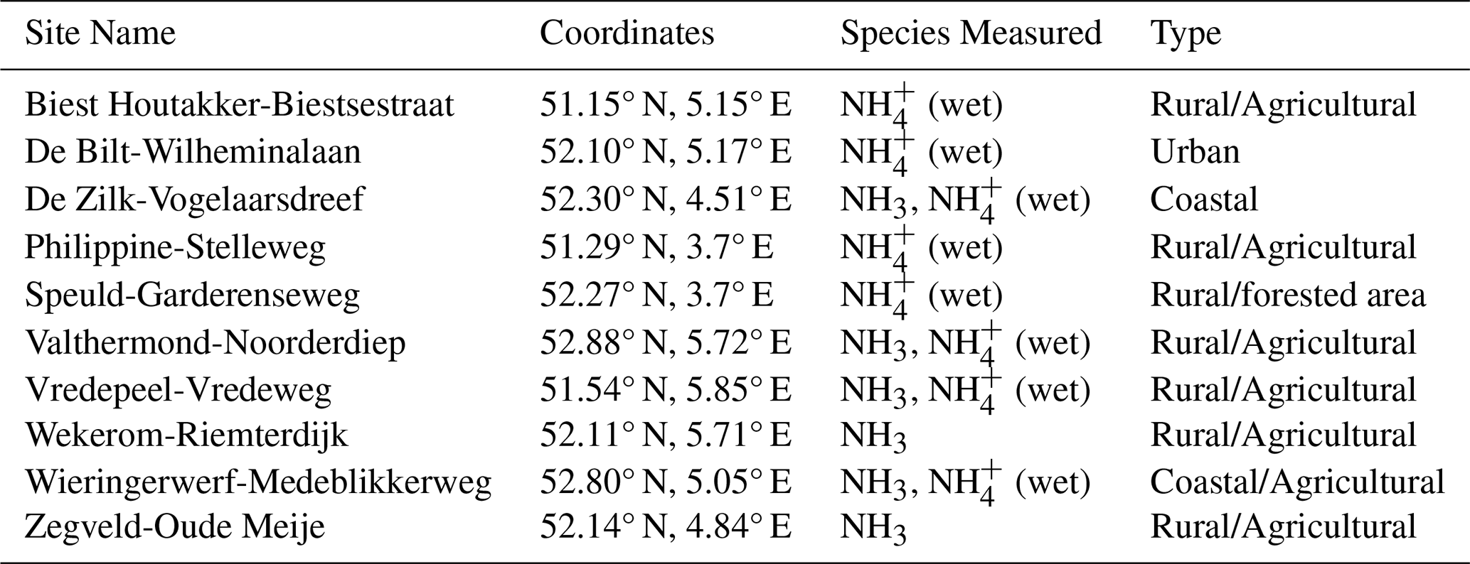
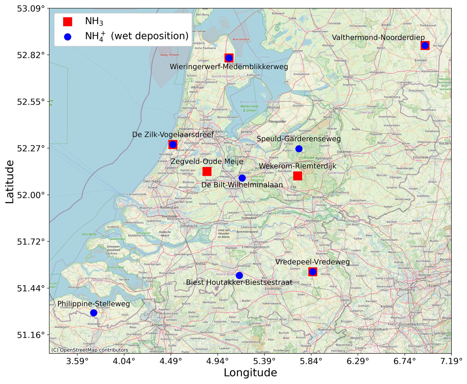
Figure 1Map of the locations of the selected LML sites in the Netherlands used for comparisons with the model simulations. Underlying basemap data sourced from OpenStreetMap contributors (2017).
The NH3 measurement sites occasionally experience local-scale enhancement events (i.e. nearby manure dumping events), which are not spatially representative of the model resolution. For 2020 onward, official flags are provided in the LML dataset to enable the filtering of such events, but for the years prior to this no such information is available. As a result, additional filtering was manually applied, and any hourly NH3 observations with concentrations exceeding 100 µg m−3 are removed and excluded from the comparisons.
2.3.2 The MAN network
The “Measuring Ammonia in Nature” (MAN) network was established in 2005 to monitor atmospheric ammonia concentrations in nature reserve areas across the Netherlands, with a particular focus on nitrogen-sensitive Natura 2000 areas (Lolkema et al., 2015). The network provides essential data for assessing national ammonia concentration trends, validating air quality models, and analyzing regional variability.
The network employs commercial Gradko passive ammonia samplers, which are cost-effective, easy to deploy, and well-suited for large-scale monitoring (Lolkema et al., 2015; Noordijk et al., 2020). These samplers are calibrated monthly using active ammonia sampling devices within the LML network (Lolkema et al., 2015). Local volunteers, often conservation wardens, handle the monthly exchange of samplers, ensuring consistent data collection across diverse habitats.
Currently, the MAN network includes over 300 sampling sites across the Netherlands. The ammonia concentration data gathered by the network facilitates the identification of spatial concentration patterns and regional anomalies throughout the country. Note that in comparison to LML, the MAN samplers are typically placed in nature areas and away from source regions.
The MAN network's data plays a critical role in assessing the effectiveness of environmental policies aimed at reducing nitrogen emissions and in analyzing long-term trends in nitrogen deposition. The network can detect annual trends as low as 3 % over extended time series, making it a valuable tool for air quality management and biodiversity conservation in nitrogen-sensitive areas (Lolkema et al., 2015).
To reduce meteorological influences on the passive samplers, the MAN network is calibrated against high-performance reference instruments for NH3 at six locations in the Netherlands (see Berkhout et al., 2017). The calibration process is detailed in Noordijk et al. (2020). The uncertainty in the MAN measurements consists of two components: the measurement uncertainty and the calibration uncertainty. The random uncertainty is approximately 0.9 µg m−3 for a single monthly value and 0.32 µg m−3 for annual averages. The systematic uncertainty is estimated at 28 % for monthly values and 10 % for annual averages (Noordijk et al., 2020).
For comparison with the LETKF simulations, all available MAN data from the period 2018–2022 was used, comprising a total of 309 standard sites, and 6 additional MAN calibration sensors located at LML measurement sites. While not all sites provide uninterrupted time series over the full period, the large number of sites and monthly measurements ensures statistically robust results.
3.1 Optimized emission fields
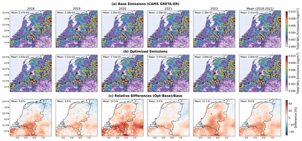
We first examine the NH3 emission fields pre- and post-assimilation to evaluate the impact of ingesting satellite observations on the model simulation. The base and LETKF-optimized NH3 yearly total emissions for each individual year and for the mean over 2018–2022 are shown in Fig. 2. Unless otherwise stated, the LETKF-optimized simulation refers to the main co-assimilation run using NH3 observations from IASI and CrIS together with NO2 observations from TROPOMI. The relative-difference plots in Fig. 2c reveal a consistent spatial pattern: increases across much of the south and east of the Netherlands and decreases in the north and the adjacent regions of Germany. The largest mean increase occurred in 2020 (+14.3 %), the smallest in 2021 (+3.0 %), with a period-average change of +8.0 %. The relative-difference panels in Fig. 2c should therefore be interpreted together with the underlying base and optimized emission fields in Fig. 2a and b, since large percentage changes can still correspond to modest absolute changes where baseline emissions are low. It should be noted that 2020 was an exceptional year, with unusually warm and sunny summer months, which in turn led to increased volatilization of NH3 and higher emissions. This is likely one of the key factors contributing to the higher emissions change post-assimilation in that particular year.
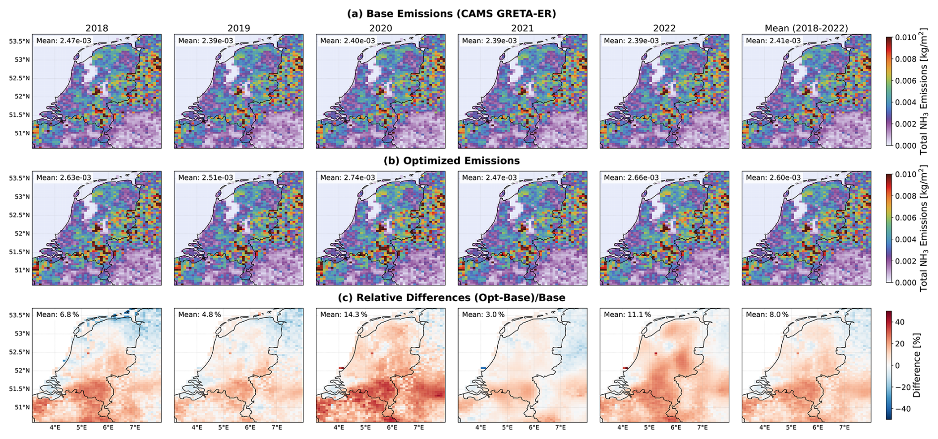
Figure 2(a) The total NH3 emissions by year and the mean emissions 2018–2022 period from the base CAMS GRETA-ER inventory, (b) the same but for the optimized emissions from the LETKF analysis, and (c) the mean relative differences between the base and the optimized emission fields.
The persistent increases in the south-eastern Netherlands mirror the patterns reported by Ge et al. (2020), who found that incorporating detailed agricultural activity data into the Monitoring Atmospheric Composition and Climate (MACC) inventory led to higher emissions in this region due to improved spatial allocation of sources, more accurate representation of manure management and application timing, and region-specific regulatory constraints. They also showed that emissions here are disproportionately influenced by intensive pig and poultry farming, whereas dairy cattle dominate in much of the rest of the country. In contrast, the decreases we find in the north are consistent with their observation that refined allocation can reduce emissions where earlier inventories overestimated activity, particularly for dairy cattle. These parallels suggest that the positive adjustments in our assimilation likely reflect structural biases in the base inventory, both in the spatial distribution and the livestock-sector partitioning of emissions, rather than being solely an artifact of the assimilation.
Meteorological effects can also have a significant impact on NH3 emissions, with temperature, precipitation, and wind speed strongly influencing volatilization rates and atmospheric transport (Søgaard et al., 2002; Gyldenkærne et al., 2005; Ge et al., 2023). Warm, dry conditions can substantially enhance emissions above climatological norms, while precipitation events may suppress them or trigger post-event peaks. Such variability may contribute to the year-to-year differences in our assimilation adjustments, and could help explain the particularly large increase in 2020, when the Netherlands experienced a very sunny spring and an unusually warm, dry summer.
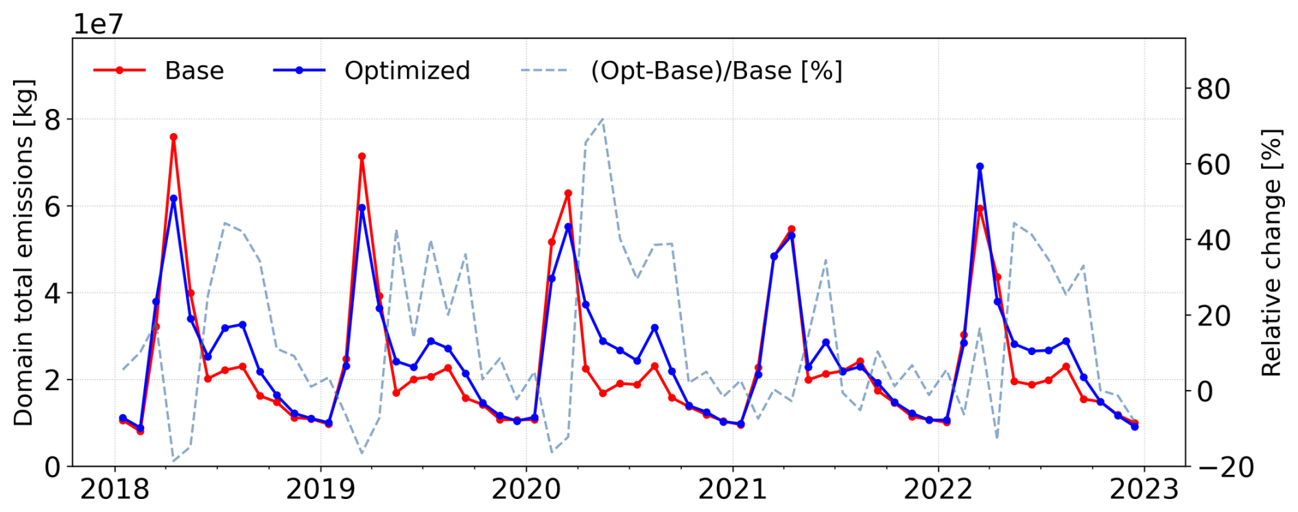
Figure 3A time-series of monthly total NH3 emissions calculated over the model domain shown in Fig. 2 for the 2018–2022 period from the base simulation and the optimized LETKF simulation. The relative difference (optimized – base)/base in % is shown by the dashed line.
In addition to the annual emission changes, it is also informative to examine the temporal evolution of emissions at finer timescales. Figure 3 presents the time series of monthly NH3 emission totals, aggregated over the same region shown in Fig. 2, and provides further insight into how the assimilation influences variability across individual months. The base emissions show a similar seasonal cycle in all years, characterized by a pronounced spring peak and a smaller secondary peak in summer. This double-peaked seasonal cycle likely reflects the combination of the prescribed seasonal timing in the agricultural NH3 emission parameterization and meteorologically driven variability in NH3 volatilization under warmer conditions. Relative to the base simulation, the optimized emissions show a broadly consistent pattern of changes across all years, with a reduction in the spring peak and a corresponding increase during the summer months. Particularly large decreases in the spring peaks are seen for 2018–2020, whereas only a minimal decrease occurs in 2021 and a slight increase is found in 2022. As seen in Fig. 3, 2020 exhibits the largest emissions changes, with particularly large increases in the emissions (on the order of +70 %) in the LETKF-optimized simulation between April and September. In contrast, 2021 shows the smallest emissions changes, with a smaller-than-average increase in the emissions in the optimized simulation in May and June, but mostly minor changes throughout the remainder of the year.
Similar NH3 seasonal cycles to that of the optimized simulation have been presented in recent modeling and observational studies of the region. The updated temporal emission profiles presented by Ge et al. (2020), and which are implemented in the model simulations used in this study, show shifts in the early-year emission peaks to later in the springtime, and increases in the overall summertime emissions. A long-term time-series (2008–2020) of IASI NH3 total column measurements over the Netherlands in Van Damme et al. (2022) displays a springtime peak in April and a slightly smaller but somewhat comparable secondary peak in July to August. A similar pattern of reduced spring peaks and enhanced summertime emissions was also found by Ding et al. (2024) after assimilating CrIS NH3 observations into the DECSO system. In addition, a recent two-year field campaign in key agricultural regions of the Netherlands by Lô et al. (2025) observed strong peaks in surface NH3 concentrations during the summer months, driven by increased volatilization under warmer conditions. Despite the inclusion of the Ge et al. (2020) temporal profiles, the model simulations in this study still underestimate summertime emissions relative to these independent datasets, suggesting that the seasonal emission distribution in LOTOS-EUROS may require a further upward adjustment during summer. The broadly consistent pattern of change across most years in Fig. 3 supports the need to shift emissions from early spring toward the summer months to better align the model with satellite and in-situ observations.
3.2 Impact on NHx deposition fields
Maps of the total NHx deposition for the base and optimized simulations are shown in Fig. 4a and b. The relative-difference plots in Fig. 4c display a similar general spatial pattern as for emissions, whereby the largest increases in the modeled deposition occur in the south and east of the Netherlands, while smaller or negative differences are found in the north of the country. The largest changes in the total deposition are seen in 2020 and 2022 with differences of +10.4 % and +9.6 %, respectively. Very small relative differences are seen in 2019 and 2021 of +3.8 % and +2.7 %, respectively. The mean relative change in the NHx deposition over the full 2018–2022 period is +6.3 %. It should be noted that a large relative difference is seen over the area of the IJsselmeer and along the Dutch coastline that is caused by the dry re-emission of NHx , which is derived from standard maps in the LOTOS-EUROS model. However, the absolute differences (in terms of kg m−2) in these areas are negligible. The reduced sensitivity of deposition to the assimilation is expected, since part of the emitted NH3 is exported offshore.
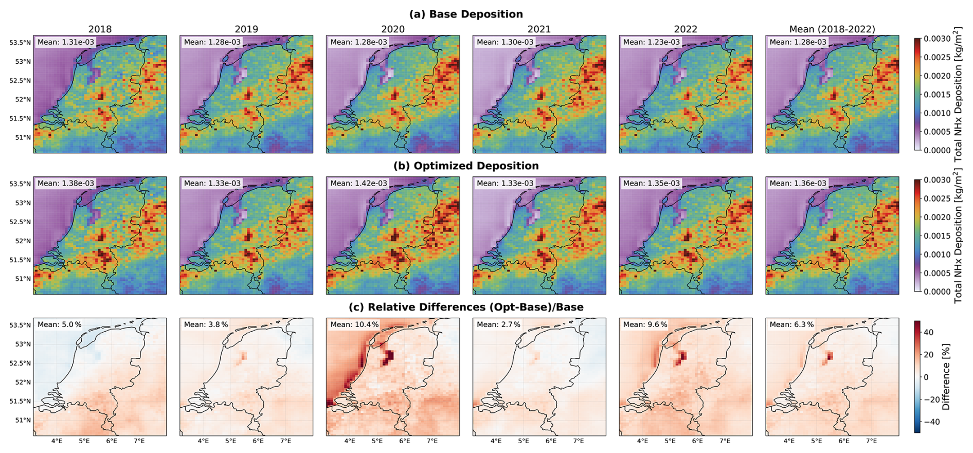
Figure 4(a) The modeled total NHx deposition (dry + wet) by year and the mean for the 2018–2022 period from the base simulation, (b) the same but for the optimized deposition from the LETKF assimilation run, and (c) the mean relative differences between the base and the optimized deposition fields.
3.3 Spatial distribution of NH3 Concentrations
In this section, we evaluate the effects of the assimilation on the spatial distribution of NH3 concentrations. Figure 5 shows the spatial distribution of NH3 total column concentrations over the model domain from 2018 to 2022, comparing the base and optimized simulations. Panels a on the top row present the NH3 total columns from the base model, panels b on the middle row show the updated concentration fields after integrating satellite observations, and panels c on the bottom row display the relative differences, highlighting the assimilation's impact on simulated NH3 concentrations. Across all years, both the baseline and optimized NH3 total column fields exhibit similar large-scale spatial patterns, with elevated NH3 levels concentrated in regions known for intensive agricultural activity, such as northwestern Germany, and the south-eastern Netherlands. However, clear differences emerge between the prior and assimilated estimates, with the assimilation generally increasing NH3 concentrations across most regions, as shown by the predominantly positive relative differences in panels c. The largest change in the total columns between the base and optimized simulations is seen in 2020, where a mean increase of 29.3 % is found, while the years with the smallest differences were 2019 and 2021 where an increase in the columns across the domain of roughly 3.5 % in both years was found. The mean differences over the 2018–2022 period indicate a systematic increase in mean NH3 column concentrations within the model domain of approximately 10.4 %, with the largest increases seen over the south eastern Netherlands, suggesting that the base model likely underestimates emissions or overestimates deposition processes there. Likewise, the relative-difference panels in Fig. 5c should be interpreted in the context of the underlying base and optimized total-column fields in Fig. 5a and b, since the largest percentage changes do not always coincide with the largest absolute concentration changes. In some areas, namely in the northern and southern western parts of the domain in 2018 and 2019, slight reductions in the NH3 total columns are seen after assimilation, which is likely due to an overestimation in the a priori emissions, and this broadly mirrors the pattern of the emissions changes from Fig. 2. For 2020 and 2022, the mean differences in NH3 total columns are positive across the domain, whereas the corresponding emission difference maps show localized decreases, particularly in the northeastern part of the model domain. This apparent mismatch likely reflects the influence of atmospheric transport, as NH3 emitted in one region can be advected and deposited elsewhere, so column enhancements do not necessarily coincide spatially with the emission sources. The mean of the differences for all years reveals a relatively consistent year-to-year pattern of enhancement, reinforcing the robustness of these corrections over multiple years. The systematic increases in NH3 after assimilation suggest that satellite-derived observations are providing important constraints to correct for underestimation in the base model and emissions, particularly in regions where agricultural sources dominate. These adjustments likely reflect the assimilation compensating for structural model biases such as underestimated volatilization, overly rapid deposition, spatial misallocation in emission inventories, or the fact that the current temporal NH3 agricultural emission profiles do not take meteorological conditions sufficiently into account (Ge et al., 2023). As discussed in Sect. 2.2, satellite retrievals can carry systematic biases arising from factors such as a priori assumptions, poor observational conditions (e.g. low thermal contrast), or cloud screening, which may influence the resulting analysis fields. By assimilating several satellite datasets, the impact of biases in individual datasets can be reduced to some extent, and this will be explored in further detail in Sect. 3.5.2. Additional support for the temporal behavior of the optimized NH3 concentration fields is provided by the monthly MAN time series shown in Appendix Figs. B2 and B4, although these comparisons are discussed in detail later in Sect. 3.5.4.
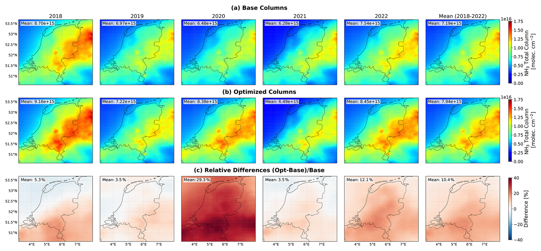
Figure 5(a) The mean NH3 total column concentrations by year and for the full 2018–2022 period for the LOTOS-EUROS baseline simulation, (b) the same but for the LETKF optimized simulation, and (c) the mean relative differences between optimized and baseline simulations.
3.4 Averaging kernel sensitivity and observation density
To evaluate the impact of the number of available satellite observations on the assimilation, we examine the local observational constraint on the NH3 emission adjustment factors using the averaging kernel sensitivity. Following Chen et al. (2023), the averaging kernel matrix is defined as
where I is the identity matrix, is the posterior error covariance matrix, and Sa is the a priori error covariance matrix, both of which are directly output per time step from the LETKF. In the scalar case considered here, this reduces locally to the diagonal element , where sa and sf are the local analysis and forecast error variances, respectively. The mapped values shown below therefore represent the local averaging kernel sensitivity at each grid cell and time step, expressed as percentages. Strictly speaking, the degrees of freedom for signal (DOFS) are given by the trace of A (Chen et al., 2023).
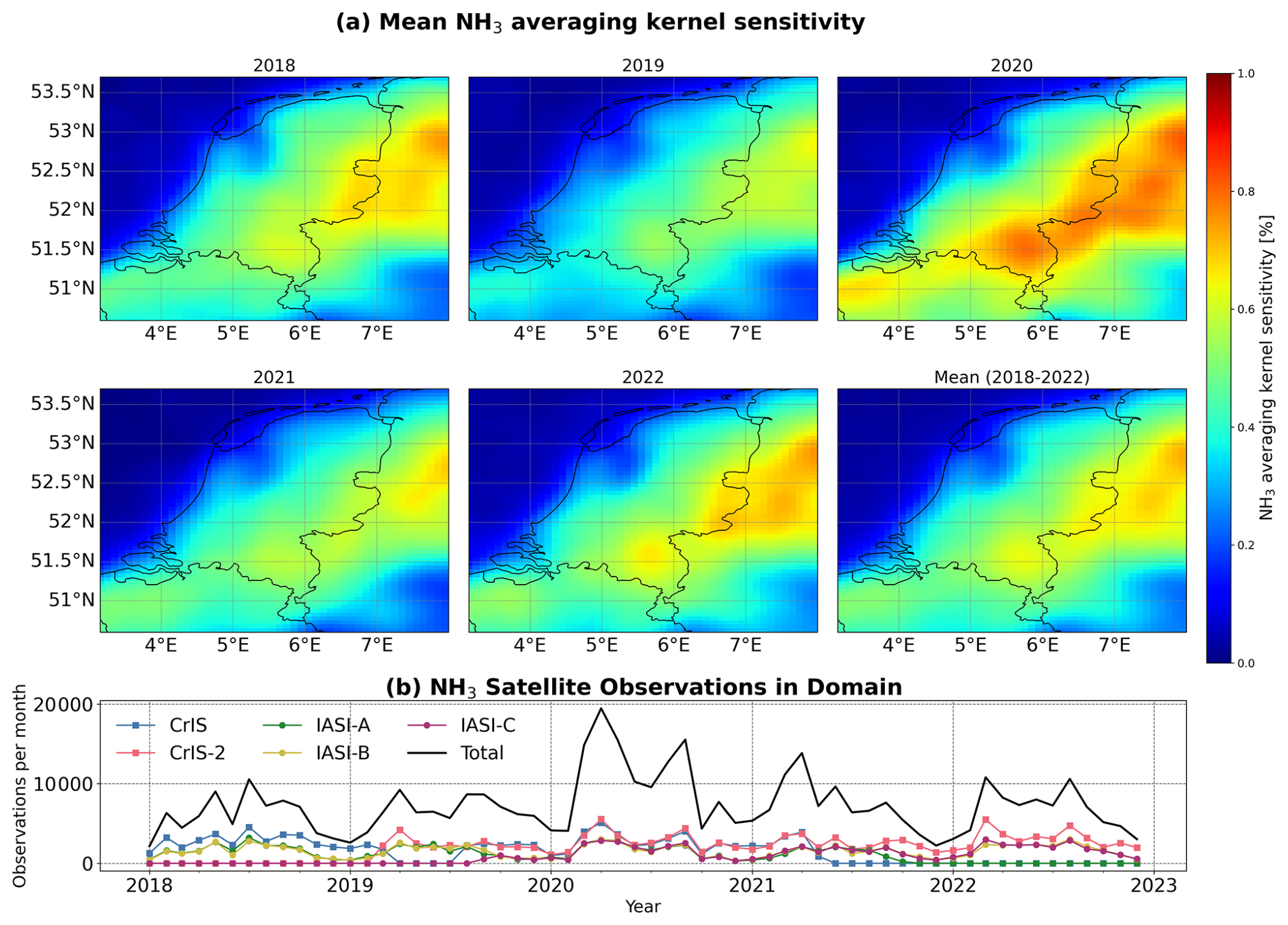
Figure 6(a) The mean NH3 averaging kernel sensitivity (%) in the model domain, and (b) a time series of the number of NH3 satellite observations per month within the domain. The total number of observations per month is shown by the solid black line.
Figure 6a presents the mean spatial distribution of the averaging kernel sensitivity for each simulation year, as well as the mean over the full 2018–2022 period. Regions with broad observation coverage and high sampling density, particularly over areas with higher NH3 concentrations, where retrieval sensitivity is generally greater and retrieval uncertainties are lower, exhibit elevated averaging kernel sensitivity values, indicating a stronger observational influence. Conversely, regions with sparse observations, such as areas with lower retrieval sensitivity, show lower values, implying a stronger dependence on the model prior. A consistent pattern of higher averaging kernel sensitivity is seen in the northwestern German border region and throughout much of the Netherlands, particularly along the western half of the country, in all years. In addition, higher mean averaging kernel sensitivity is seen in 2020, when the overlap between the CrIS and IASI instruments was greatest, as reflected in Fig. 6b. The CrIS-2 NH3 data product begins in March 2019 and CrIS-1 observations end in mid-2021 as a result of the instrument being decommissioned, while the IASI-C NH3 data product starts in September 2019 and the IASI-A product ended in October 2021 due to the MetOp-A platform reaching the end of its operational lifetime.
To assess the relationship between averaging kernel sensitivity and observation density, a time series of the total number of observations in the model domain is shown in Fig. 6b. The higher mean averaging kernel sensitivity in 2020 coincides with the period of greatest overlap in CrIS and IASI availability, suggesting that increased observation coverage contributed to stronger observational constraint in that year. This impact is also consistent with Figs. 2 and 5, where the largest adjustments in emissions and total column concentrations relative to the original simulation were observed in 2020. It is possible that in years with more limited observations, the post-analysis emission changes are underestimated because less observational information is available to constrain the system. However, as discussed earlier, 2020 was also an exceptional year with very warm summer months and particularly high NH3 emissions, which likely also contributed to the higher averaging kernel sensitivity. The relationship is therefore not strictly linear, since the averaging kernel sensitivity depends not only on observation count, but also on the prior and posterior error covariance structure and on the relative uncertainty of the satellite retrievals. This means that the assimilation can be limited both by the density of available retrievals and by their accuracy: high observational coverage with large uncertainties provides limited benefit, whereas accurate retrievals at low coverage can still meaningfully constrain the system, but are less able to capture transient emission events or resolve daily and diurnal cycles. In practice, both factors act together, and the results emphasize the importance of maintaining dense, accurate satellite observations, ideally from multiple instruments, to more effectively constrain NH3 emissions and capture interannual variability.
3.5 Comparisons with ground-based observations
Although the assimilation produces consistent adjustments to the modeled emissions, concentrations, and to a lesser extent the deposition fields across the simulation period, independent evaluation against ground-based observations is needed to assess the extent to which these optimized fields represent an improvement over the original simulation.
3.5.1 LML hourly surface concentrations
To accurately assess the impact of the assimilation of the satellite observations, and to evaluate whether the optimized concentration fields represent more realistic estimates of the true spatio-temporal distribution of NH3, it is important to compare the results against an independent dataset. The surface concentrations from the base and optimized model runs were compared against ground-based surface observations from six sites in the LML network that were described in Sect. 2.3.1. These sites were selected because they provide hourly NH3 surface concentration measurements and have significant time-series (i.e. >1 year) of data. As the primary focus of this study is NH3, detailed discussion of the corresponding NO2 assimilation results is beyond the scope of the present study. These results will be presented separately in a forthcoming paper to allow for a more comprehensive treatment.
A correlation plot of the monthly temporal comparison is shown in Fig. 7, and a corresponding plot of the spatial means (i.e. all sites averaged for a given month) is provided in Fig. 8. These two summary views are shown separately to distinguish temporal agreement at individual sites from agreement in the spatial pattern across the Dutch monitoring network. They provide compact statistical summaries, while complementary temporal and spatial context is given by the diurnal-cycle analysis and the mapped concentration fields shown elsewhere in the manuscript. All linear regressions were performed using an ordinary least squares fitting approach. Uncertainty estimates are reported for the statistical quantities shown in the model–observation scatter-plot comparisons. Unless otherwise stated, uncertainties correspond to one standard error. For the mean bias, μ, the uncertainty was estimated as , where sd is the sample standard deviation of the model–observation differences and N is the number of paired data points. For the standard deviation of the differences, σ, the standard error was approximated as , assuming normally distributed differences. For the Pearson correlation coefficient, R, uncertainties were estimated using the Fisher transformation, with standard error in Fisher-z space and then transformed back to correlation space. Uncertainties in linear regression slopes were estimated from the ordinary least-squares covariance matrix. These uncertainty estimates assume independent paired samples and should therefore be interpreted as approximate, particularly for comparisons involving repeated monthly values across sites. For changes between the base and optimized simulations, statistical robustness was assessed using paired bootstrap resampling of the matched observation, base-model, and optimized-model triplets; changes were considered statistically significant when the 95 % bootstrap confidence interval did not include zero. The main surface NH3 comparison statistics are summarized in Table 2, while the full surface-concentration uncertainty estimates and bootstrap confidence intervals are provided in Appendix Tables C1 and C2. Corresponding uncertainty estimates and bootstrap confidence intervals for the wet deposition comparisons are provided in Appendix Tables C3 and C4. Uncertainty estimates for the 2020 satellite-subset sensitivity experiments are provided in Appendix Table C5.
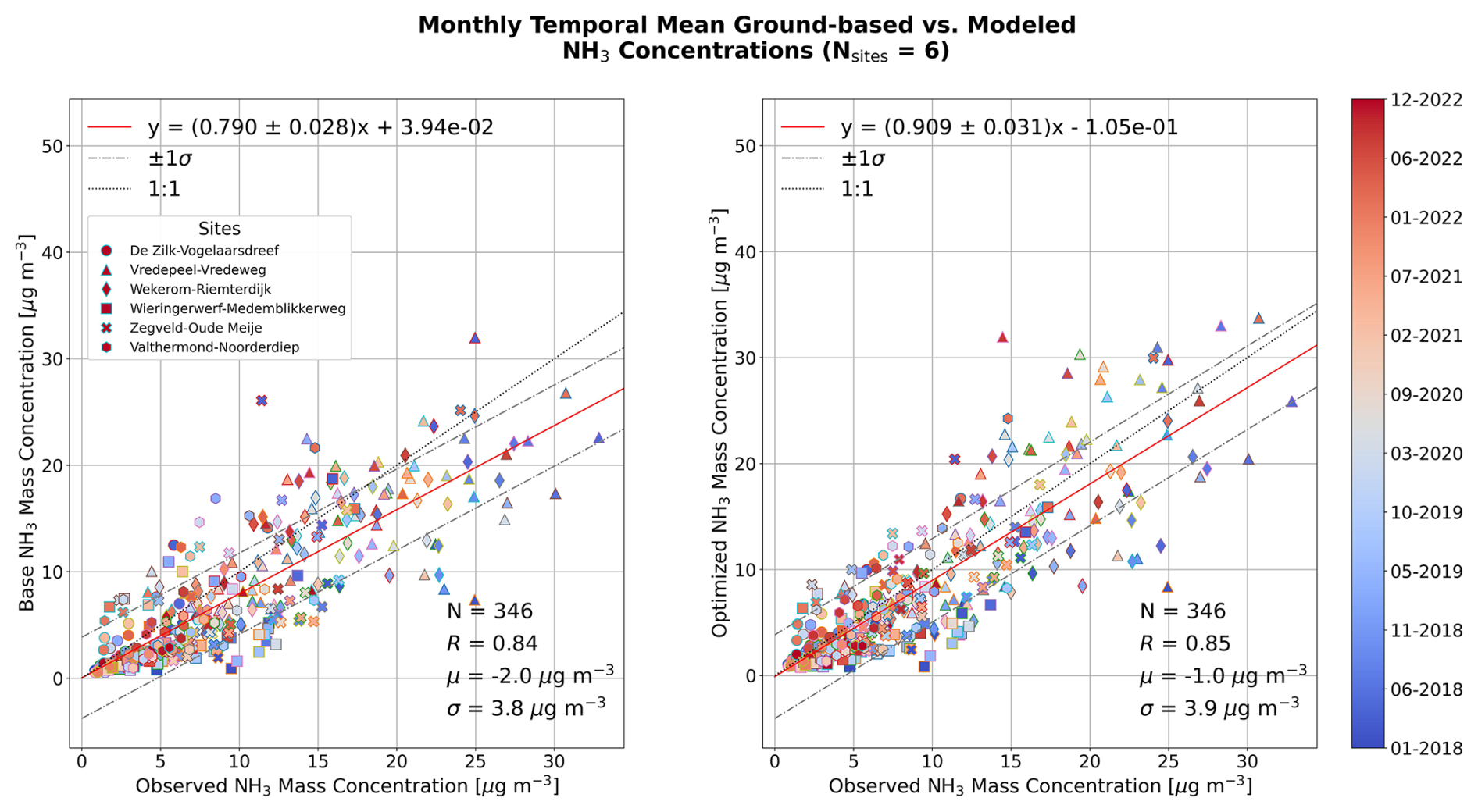
Figure 7Scatter plot of monthly temporal means of (left) LOTOS-EUROS base NH3, and (right) LOTOS-EUROS LETKF optimized NH3 vs. LML observed NH3 surface concentrations for the period of January 2018–December 2022. Uncertainty estimates for the reported statistics and paired bootstrap confidence intervals for optimized-minus-base changes are provided in Appendix Tables C1 and C2.
Table 2Summary of model performance statistics for NH3 surface concentration comparisons against LML and MAN observations for the 2018–2022 period. Reported values correspond to monthly spatial-mean comparisons. Values for the slope, mean bias (μ), and spread of model–observation differences (σ) are reported as estimate ± one standard error. Confidence intervals for R correspond to the 95 % interval obtained using the Fisher transformation.
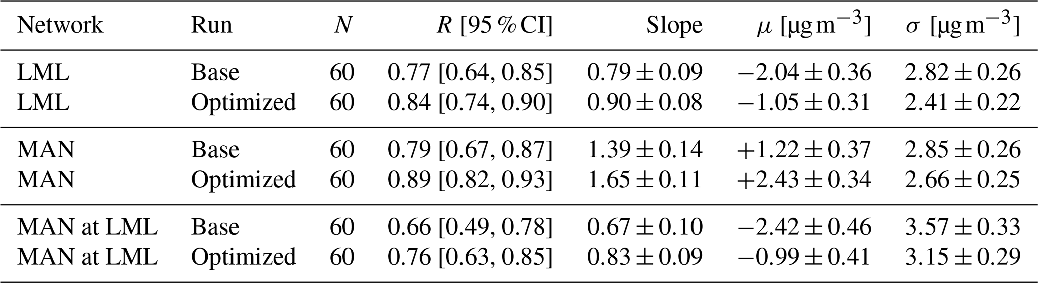
Not all LML sites provided data for all months, leading to a total of 346 data points compared with the expected 360 in Fig. 7. For the LML temporal comparison, the assimilation produces a statistically robust reduction in mean bias and a significant improvement in the regression slope, while the already high temporal correlation remains statistically similar before and after assimilation. The bias decreases from to µg m−3, and paired bootstrap resampling indicates that this change is significant at the 95 % level ( µg m−3, 95 % CI: +0.74–+1.25 µg m−3). The regression slope increases from 0.790±0.028 to 0.909±0.031, also representing a statistically significant improvement (, 95 % CI: +0.062–+0.173). In contrast, the change in correlation from R=0.836 [0.801, 0.865] to R=0.846 [0.813, 0.874] is not statistically significant (, 95 % CI: −0.012–+0.040). For the monthly spatial means shown in Fig. 8, the assimilation again produces a statistically significant reduction in mean bias, from to µg m−3 ( µg m−3, 95 % CI: +0.54–+1.44 µg m−3). The Pearson correlation and regression slope also increase, from R=0.765 [0.635, 0.853] to R=0.837 [0.740, 0.900] and from 0.787±0.087 to 0.895±0.077, respectively. However, paired bootstrap confidence intervals for these changes include zero (, 95 % CI: −0.002–+0.146; , 95 % CI: −0.028–+0.236), so these increases should be interpreted as suggestive rather than statistically significant at the 95 % level. The LML comparison therefore indicates that the most robust improvement is the reduction of systematic underestimation, with additional but weaker evidence for improved spatial agreement.
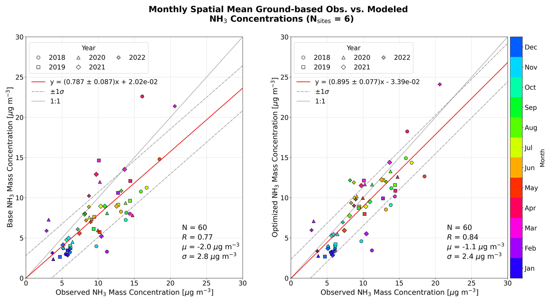
Figure 8Scatter plot of monthly spatial means of (left) LOTOS-EUROS base NH3, and (right) LOTOS-EUROS LETKF optimized NH3 vs. LML observed NH3 surface concentrations for the period of January 2018–December 2022. Each data-point represents the mean calculated across all LML sites for a given month, and are colored corresponding to the month while the marker style indicates the year. Uncertainty estimates for the reported statistics and paired bootstrap confidence intervals for optimized-minus-base changes are provided in Appendix Tables C1 and C2.
A Taylor diagram illustrating the measurement-model comparisons for the base and optimized simulations at each individual LML site is shown in Fig. 9. In general, the correlations between the measured and modeled surface NH3 concentrations are higher for the optimized run at all LML sites except Wekerom-Riemterdijk, with the clearest increases seen at Zegveld Oude-Meije and Valthermond-Noorderdiep. The correlation shows a small improvement at Vredepeel-Vredeweg and this was accompanied by a substantial reduction in the bias from −3.10 to 0.20 µg m−3, but a large increase in the relative standard deviation is also seen that is driven by an apparent larger number of short-term enhancement events being captured in the modeled time-series in the optimized simulation (shown in Appendix Fig. A1). The mean over all sites displays a small improvement in the correlation, but also a small increase in the standard deviation (also shown earlier in Fig. 7).
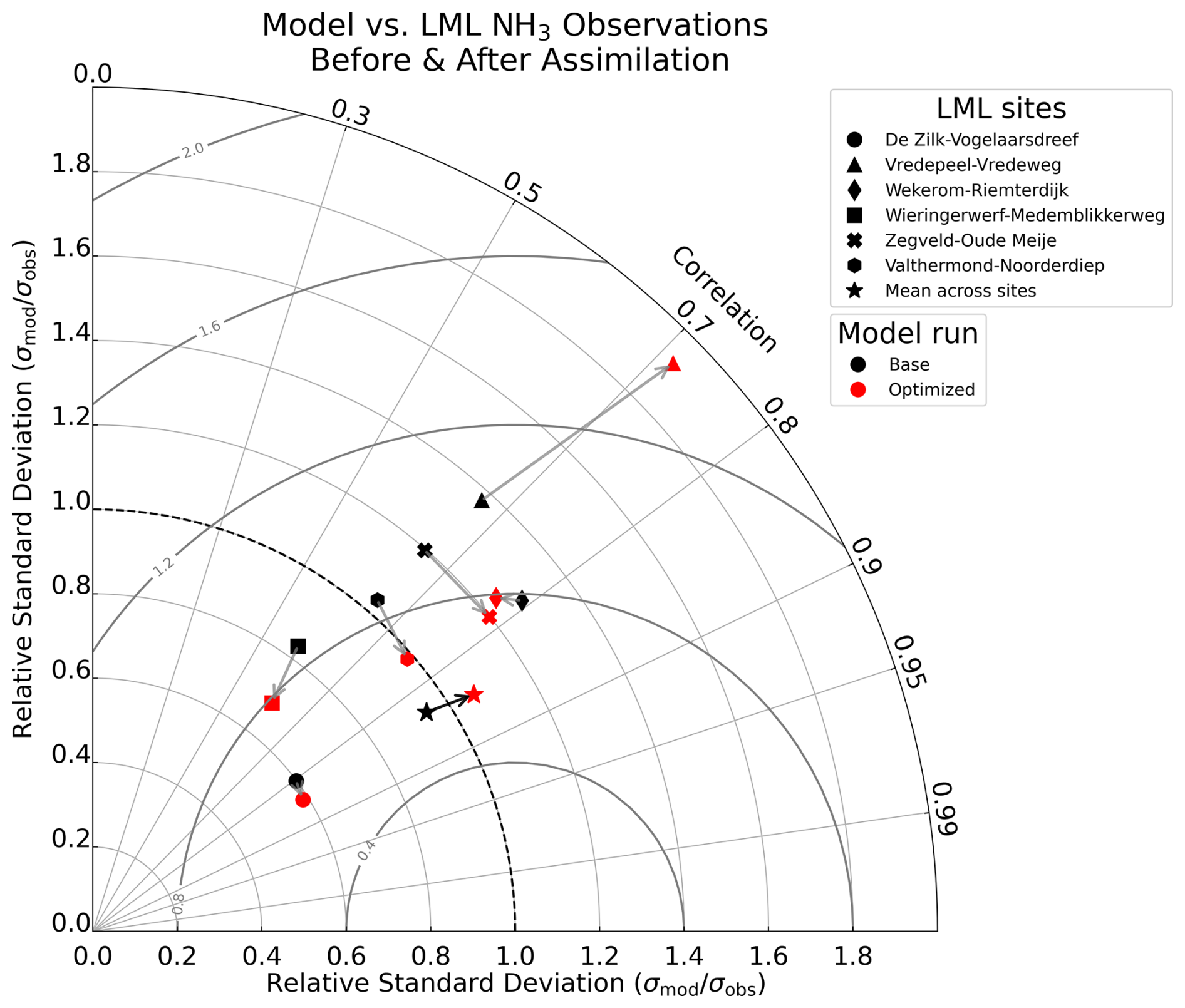
Figure 9Taylor diagram displaying the Pearson correlation coefficients and the relative standard deviations of the comparisons between the model and each LML site for the 2018–2022 period for (black) the baseline simulation and (red) the optimized simulation.
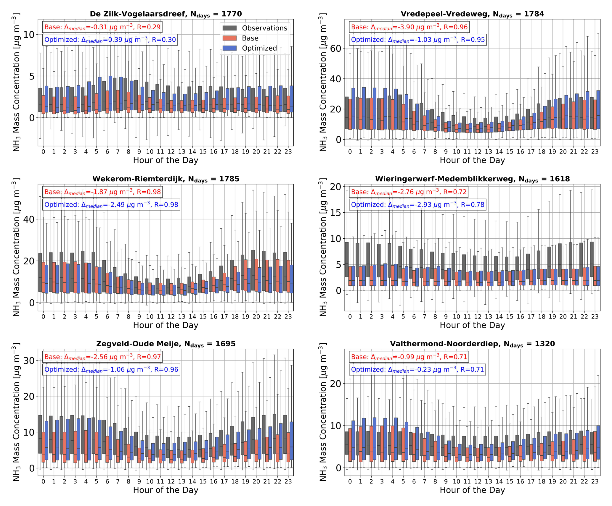
Figure 10Diurnal distributions of surface NH3 2018–2022 at each LML site from the observations (dark grey), the base model simulation (red), and the optimized simulation (blue). The box-and-whisker representation shows the distribution of hourly NH3 concentrations at each hour of the day for the three datasets. On each panel, the difference between the median diurnal cycles (Δmedian) and the Pearson correlation coefficient (R) are provided for the base run in red and the optimized run in blue.
Since the LML data are provided at an hourly frequency, the impact of assimilation on the diurnal cycles of NH3 in the model can also be investigated at each site. The mean diurnal cycles from the observations, the base model simulation, and the optimized simulation calculated over the 2018–2022 period are shown in Fig. 10. The box-and-whisker representation is used to show not only the central tendency of the diurnal cycle, but also the spread of the hourly concentration distributions at each site. In most cases, the mean differences in the diurnal cycles showed improvement relative to the observations in the optimized run in comparison to the base simulation even though only morning and afternoon satellite overpasses were used. This is partly because the effect of the assimilation persists between overpass times through the forecast step and temporal persistence of the emission adjustments, allowing the updated state to influence concentrations beyond the observation times themselves. From Fig. 10 it can be seen that in the base simulation, the diurnal cycles are in many cases largely underestimated relative to the surface observations, however after the assimilation of the satellite observations a much closer agreement between the measurements and the model is found. At Wekerom-Riemterdijk and Wieringerwerf-Medemblikkerweg the mean differences increased from −2.03 to −2.70 and −2.83 to −2.92 µg m−3, respectively. At all other LML sites a decrease in the mean difference of the diurnal cycles was observed in the optimized run relative to the base run. The correlations in the mean diurnal cycles remain largely the same, with the exception of Wieringerwerf-Medemblikkerweg where a moderate improvement from R=0.72 to R=0.77 is found. However, the diurnal cycle at Wieringerwerf-Medemblikkerweg appears to be substantially underestimated in both the base model and the optimized simulation. These underestimations are likely related to local-scale NH3 enhancements from the nearby farmlands in the Wieringermeer polder being poorly captured by the model, coupled with complex local meteorological conditions due to the proximity of the site to the IJselmeer and the North Sea which is roughly 15–20 km away.
Although the assimilation of satellite observations improves the representation of NH3 diurnal cycles relative to measurements at several LML sites, particularly with respect to systematic biases, it does not fully reproduce the observed variability. A fundamental limitation of Kalman filter–based approaches is that, although emissions are adjusted, there can be a temporal lag associated with the transport of concentrations from source regions to the measurement locations, which is strongly modulated by local meteorological conditions. Furthermore, when the underlying diurnal cycle in the model is misrepresented, assimilation at only two main satellite overpass times may be insufficient to correct these deficiencies. An additional challenge is that NH3 emissions originate from diverse sources such as livestock housing, manure application, and industry, each with distinct diurnal patterns, whereas the present assimilation setup applies a single total emission adjustment per species and grid cell, without distinguishing among source types that may have different underlying diurnal emission profiles. Overall, at sites located in regions of intensive agricultural activity such as Valthermond, Vredepeel, and Zegveld where midday enhancements are more likely to be captured by satellite observations, the influence of the assimilation on the diurnal cycles is more pronounced.
While these comparisons demonstrate clear improvements after assimilation, several further limitations should be acknowledged. First, the six LML sites provide only sparse coverage of the Netherlands and may not fully represent the strong spatial heterogeneity of NH3 concentrations across the entire country, particularly in regions with intensive agricultural emissions. Second, the model–observation comparison involves a scale mismatch: the LML instruments measure point concentrations, while the LOTOS-EUROS model output represents grid-cell averages at 7 km×7 km resolution, which can potentially introduce representativity errors. In addition, the ground-based measurements themselves are not perfect and subject to calibration uncertainties and potential interferences. Lastly, because the statistics are based on monthly averages, the analysis does not explicitly resolve short-term (daily to synoptic) variability. Consequently, part of the observed agreement may reflect the influence of meteorological variability in addition to the direct effects of the assimilation. Taken together, the LML comparisons suggest that the assimilation generally improves the agreement of the model with independent ground-based observations, particularly through a robust reduction in systematic underestimation, with weaker but positive evidence for improved spatial agreement. At the same time, the analysis also underlines the limitations of both the observational dataset and the comparison methodology, which should be taken into account when interpreting the results.
3.5.2 Impact of satellite selection on LML surface comparisons
To investigate the impact of the co-assimilation and the choice of satellites on the final optimized model state, assimilation runs were repeated for the year of 2020 using subsets of the satellite data products. These runs were: IASI only, CrIS only, and CrIS and IASI (without TROPOMI NO2), and the comparisons against the hourly LML NH3 observations were then repeated.
The temporal means for each of the four assimilation runs vs. the LML observations are shown in Fig. 11. From Fig. 11, it can be seen that relative to the other assimilation runs, the assimilation performed using IASI, CrIS and TROPOMI yields the lowest overall bias (0.1 µg m−3) relative to the LML observations while maintaining a relatively strong correlation of R=0.88. The simulation performed with IASI and CrIS without the assimilation of TROPOMI NO2 yields a higher correlation of R=0.90, but displays a higher bias of 0.7 µg m−3, a higher standard deviation, and a poorer regression slope. The simulations using only CrIS and only IASI display relatively higher mean biases of 1.4 and −1.1 µg m−3, respectively. For comparison purposes, the temporal mean comparison for the base (unoptimized) simulation for 2020 is shown in the Appendix in panel a of Fig. A2. Each of the simulations performed with assimilation show an improvement over the unoptimized base model run, which displays a correlation of R=0.82 and a mean bias of −1.9 µg m−3 relative to the LML observations.
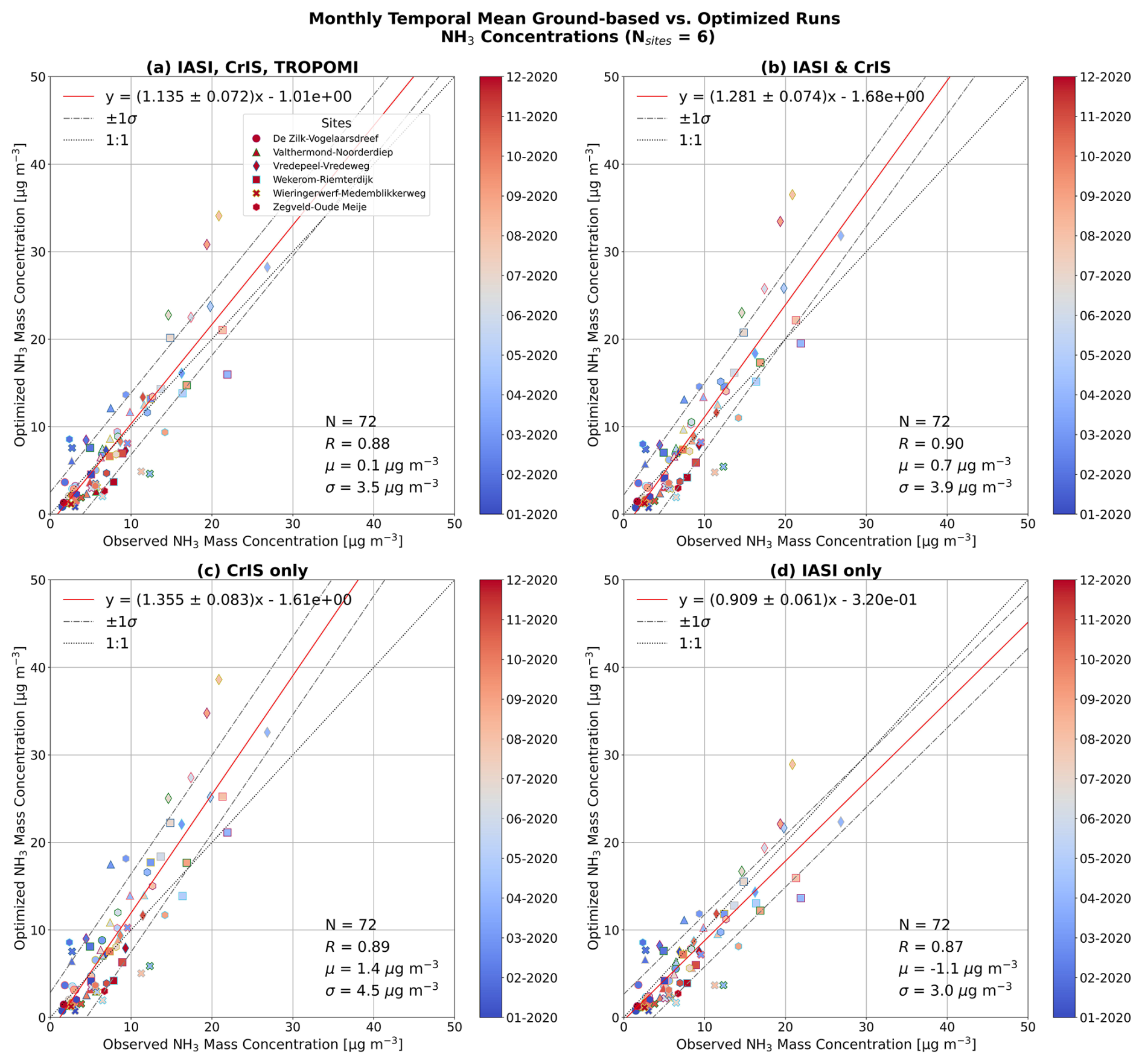
Figure 11Scatter plot of monthly temporal means of assimilation runs using (a) IASI and CrIS NH3 and TROPOMI NO2 observations, (b) IASI and CrIS NH3 observations, (c) CrIS NH3 observations only, and (d) IASI NH3 observations only vs. LML observed NH3 surface concentrations for the year of 2020. Uncertainty estimates for the reported statistics are provided in Appendix Table C5.
A similar plot of the spatial means for each of the assimilation runs vs. the LML surface observations is provided in Fig. 12. It can be seen that again from Fig. 12a, the assimilation performed using IASI, CrIS, and TROPOMI leads to the lowest overall bias (0.1 µg m−3) of the four simulations and a relatively strong correlation of R=0.90. In comparison, the assimilation run using IASI and CrIS observations but not TROPOMI has a slightly higher correlation (R=0.93), but a higher bias of 0.7 µg m−3 and a poorer slope of regression (1.163 vs. 0.977 from the IASI, CrIS and TROPOMI assimilation). The assimilation runs performed using CrIS only and IASI only (shown in panels c and d of Fig. 12, respectively) have the same or poorer correlations than the IASI, CrIS and TROPOMI run, and relatively larger biases of 1.4 and −1.1 µg m−3 for the CrIS-only and IASI-only runs, respectively. As was the case for the temporal mean comparisons, each of the optimized runs shows better agreement with the observations than the unoptimized simulation (panel b of Fig. A2), which had a weaker correlation of R=0.66 and a mean bias of −1.9 µg m−3 for 2020. Uncertainty estimates for the statistics reported in Figs. 11 and 12, together with the corresponding 2020 base-model comparison in Appendix Fig. A2, are provided in Appendix Table C5. Because these experiments are intended as a sensitivity analysis rather than a formal pairwise model-selection test, we report uncertainty estimates for each run but do not assess all pairwise differences between satellite configurations.
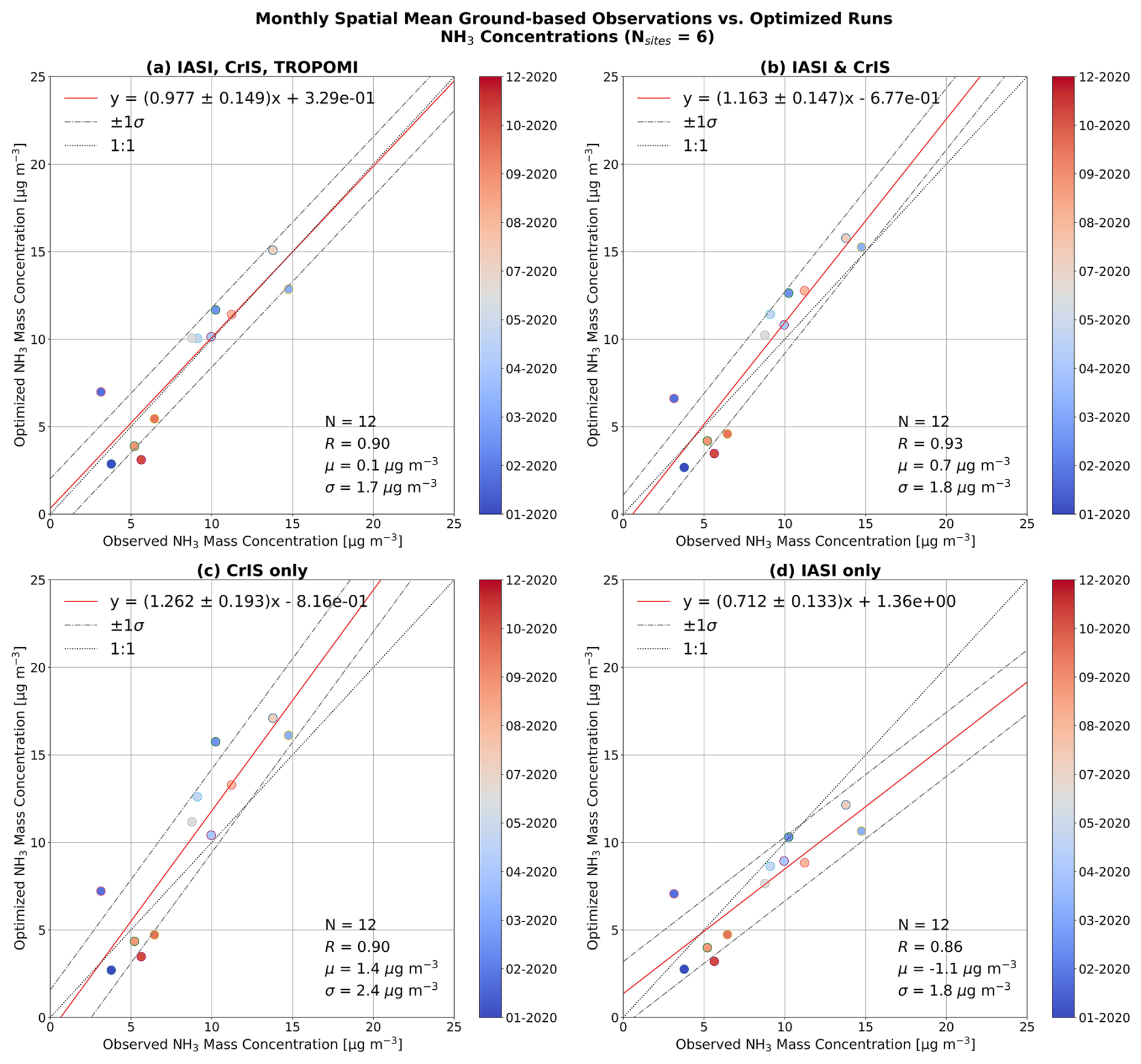
Figure 12Scatter plot of monthly spatial means of assimilation runs using (a) IASI and CrIS NH3 and TROPOMI NO2 observations, (b) IASI and CrIS NH3 observations, (c) CrIS NH3 observations only, and (d) IASI NH3 observations only vs. LML observed NH3 surface concentrations for the year of 2020. Uncertainty estimates for the reported statistics are provided in Appendix Table C5.
These comparisons highlight that the choice of satellite datasets used for assimilation is impactful, and that using just IASI or CrIS for the optimization may lead to greater biases than using a combined assimilation approach. Although assimilating a combination of CrIS and IASI observations leads to an improvement over just a single subset of the satellite data, the inclusion of TROPOMI NO2 in the optimization aids in reducing the overall biases while still maintaining a strong correlation, particularly in comparison to the un-optimized LOTOS-EUROS simulation. The added value of assimilating NO2 is that it helps to constrain the availability of HNO3 through the NO2–OH oxidation pathway, which in turn directly regulates the partitioning of NH3 into ammonium nitrate, an important sink of NH3 (Finlayson-Pitts and Pitts, 2000). In this way, the NO2 observations provide an indirect but important constraint on the fate of NH3, thereby improving the consistency of the coupled reactive nitrogen system in the model. Overall, the subset experiments indicate that the multi-satellite configuration including IASI, CrIS, and TROPOMI provides the best balance between low bias, strong correlation, and physically consistent reactive-nitrogen constraints, although the sensitivity experiments are not treated here as a formal pairwise model-selection test.
3.5.3 LML NHx wet deposition comparisons
To evaluate the impact of the assimilation on the deposition of NHx within the Netherlands, comparisons were performed against dissolved concentrations measured in precipitation. These measurements are made at irregular intervals at several LML sites, and for the comparisons, these observations were paired with the modeled deposition interpolated to a daily frequency and converted to wet deposition fluxes (in ) using the measured precipitation amounts.
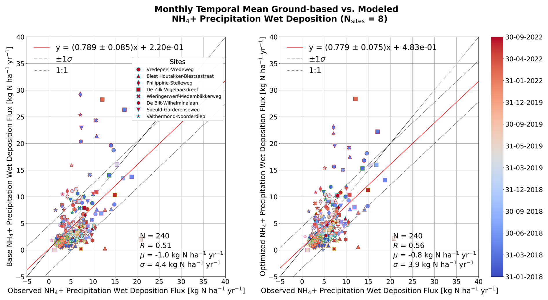
Figure 13Scatter plot of monthly temporal means of (left) base LOTOS-EUROS wet deposition flux, and (right) LOTOS-EUROS LETKF optimized wet deposition flux vs. LML surface observations for the period of January 2018–December 2022. Uncertainty estimates for the reported statistics and paired bootstrap confidence intervals for optimized-minus-base changes are provided in Appendix Tables C3 and C4.
Figure 13 shows the comparison of the measured and modeled monthly temporal means of wet deposition flux before and after assimilation. The baseline simulation displays a moderate correlation with the observations, increasing from R=0.510 [0.410, 0.598] to R=0.560 [0.466, 0.641] after assimilation. Paired bootstrap resampling indicates that this increase is statistically significant, although modest in magnitude (, 95 % CI: +0.019–+0.071). The mean bias is reduced from to , and this reduction is also statistically significant ( , 95 % CI: +0.07–+0.34 ). The spread of the model–observation differences decreases significantly from 4.40±0.20 to 3.90±0.18 ( , 95 % CI: −0.81–−0.21 ). The regression slope remains statistically similar before and after assimilation (, 95 % CI: −0.068–+0.046). The scatter plot also shows a particularly large overestimation in the modeled deposition flux for several LML sites in the spring months of 2018 and 2020, which is reduced after assimilation, while there is a general underestimation during much of the remainder of the year. A similar pattern of springtime overestimation and late-year underestimation was found in the wet deposition comparisons in the earlier LOTOS-EUROS LETKF assimilation study by Van Der Graaf et al. (2022), who attributed this behavior to a potential overestimation of springtime NH3 emissions and underestimation later in the year.
A scatterplot of the monthly spatial means is shown in Fig. 14. For this comparison, the correlation increases from R=0.578 [0.380, 0.725] to R=0.684 [0.520, 0.799], and paired bootstrap resampling indicates that this increase is significant at the 95 % level (, 95 % CI: +0.057–+0.166). The spread of the model–observation differences is also significantly reduced, from 3.04±0.28 to 2.38±0.22 ( , 95 % CI: −1.08–−0.20 ). The mean bias is reduced from to , although this change is not statistically significant at the 95 % level.
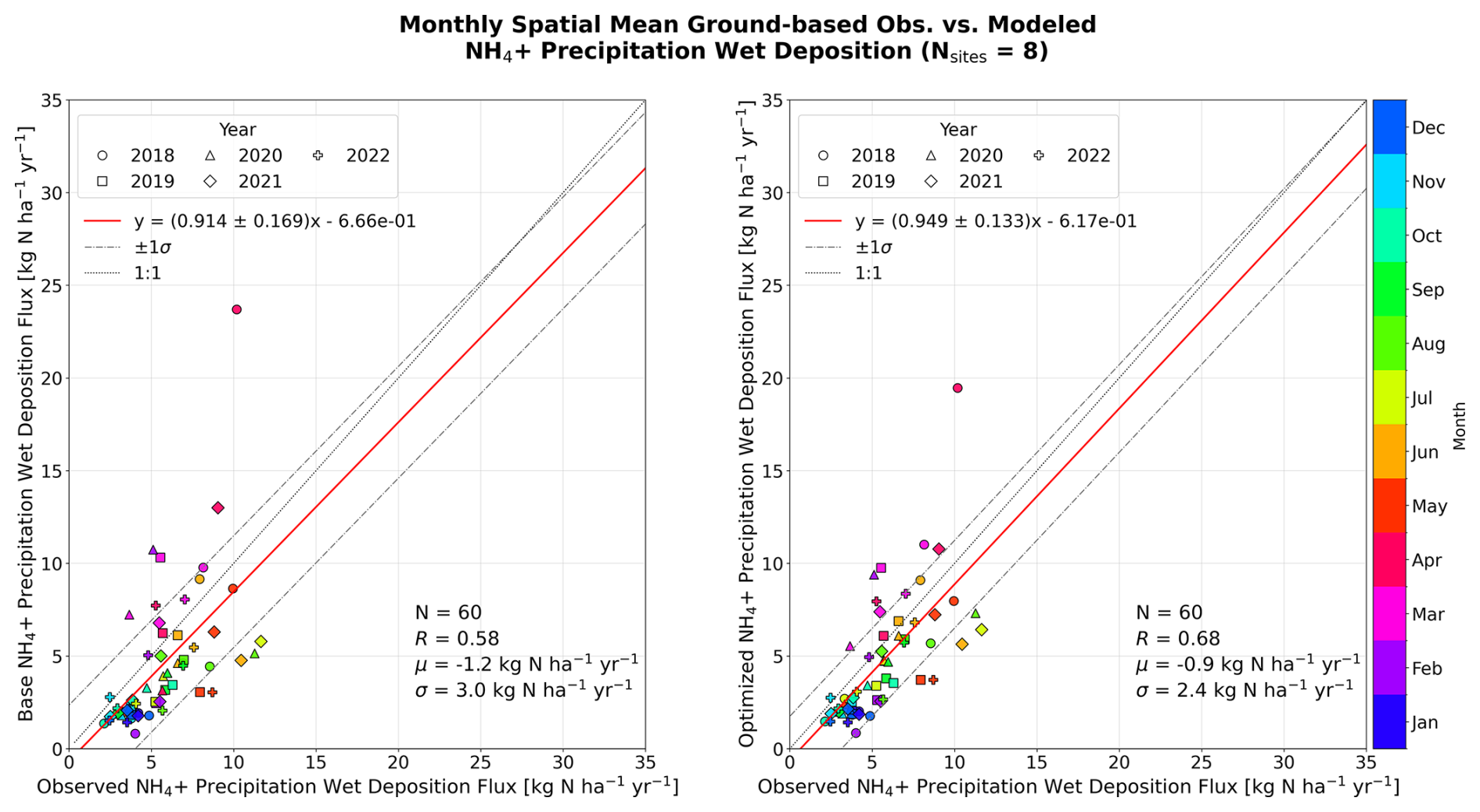
Figure 14Scatter plot of monthly spatial means of (left) base LOTOS-EUROS wet deposition flux, and (right) LOTOS-EUROS LETKF optimized wet deposition flux vs. LML surface observations for the period of January 2018–December 2022. Each data-point represents the mean calculated across all LML sites for a given month. Uncertainty estimates for the reported statistics and paired bootstrap confidence intervals for optimized-minus-base changes are provided in Appendix Tables C3 and C4.
Overall, the wet deposition evaluation provides a complementary downstream consistency check. The optimized simulation shows statistically significant improvements in the correlation, mean bias, and spread of the monthly temporal-mean comparison, as well as in the correlation and spread of the monthly spatial-mean comparison. The monthly spatial mean bias is also reduced, although this change is not statistically significant at the 95 % level. These results indicate that the assimilation improves several aspects of the modeled deposition field, but that wet deposition remains a less direct and less sensitive validation constraint than the surface NH3 concentration networks.
3.5.4 MAN monthly NH3 comparisons
The baseline and optimized simulations were also evaluated against monthly MAN NH3 surface observations from a total of 315 sites (309 standard sites, and 6 MAN instruments located at LML sites) across the Netherlands for 2018–2022. Figure 15 shows the mean observed and modeled NH3 concentrations, along with their differences. The baseline simulation exhibits a clear spatial bias, underestimation along the western coast and overestimation in the east, while the optimized run amplifies this pattern, consistent with the emission and concentration increases in the southern and eastern Netherlands. No comparable bias pattern was observed for the hourly LML sites or the CrIS and IASI total column comparisons.
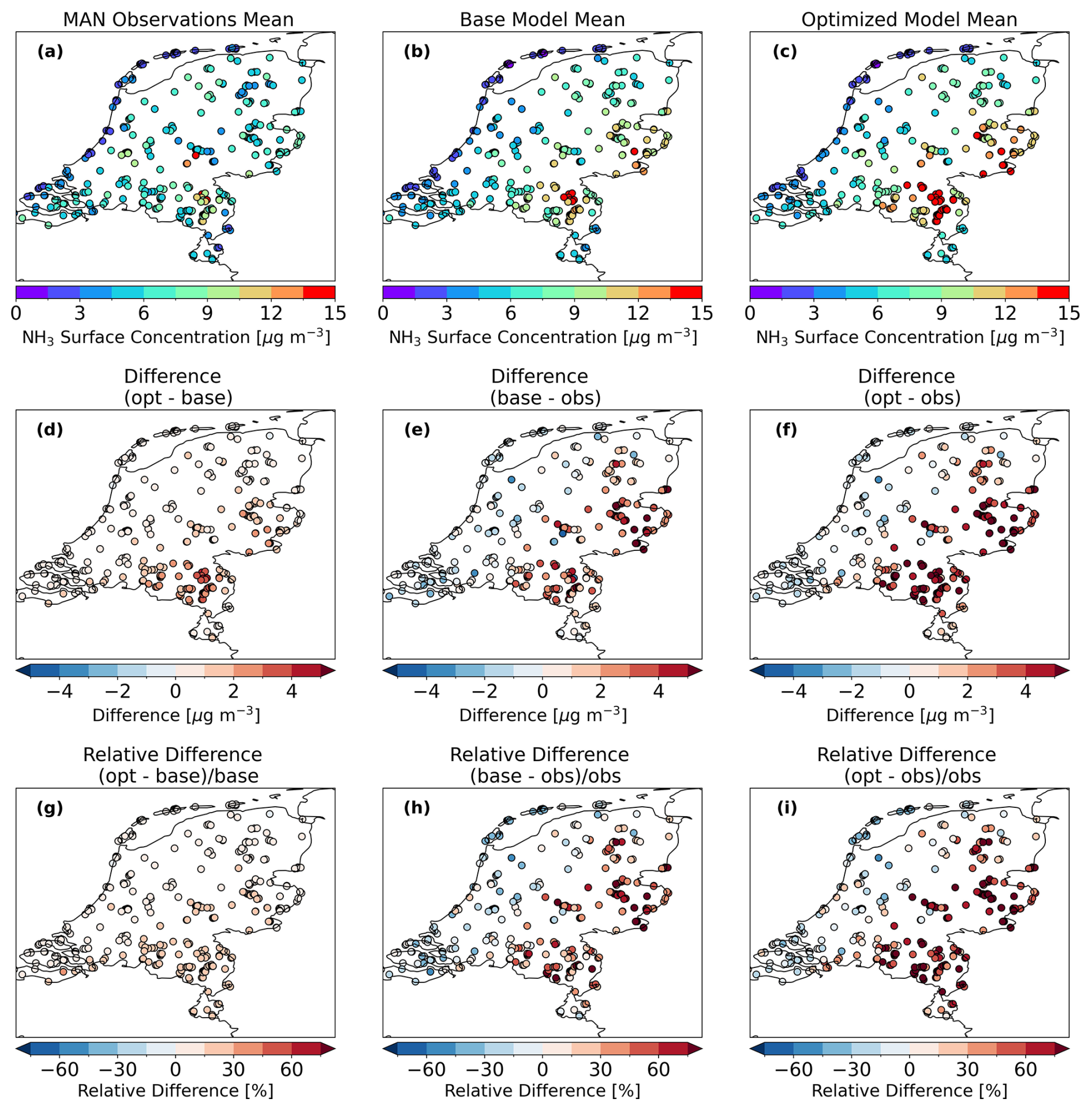
Figure 15Spatial maps of the mean NH3 surface concentrations from (a) MAN observations, (b) the base simulation, and (c) the optimized simulation calculated over the period of 2018–2022. The differences (in µg m−3) are shown in the second row for (d) the optimized run vs. the base run, (e) the base run vs. the observations, and (f) the optimized run vs. the observations, and the relative differences (in %) are shown for the same comparisons in panels (g) to (i).
Figure 16 compares monthly spatial means across all MAN sites, and for comparison purposes, the LML and MAN statistics are summarized together in Table 2. The assimilation substantially improves the spatial correlation, from R=0.791 [0.672, 0.870] to R=0.892 [0.824, 0.934]. Paired bootstrap resampling confirms that this increase is statistically significant (, 95 % CI: +0.036–+0.178). However, the improved spatial correlation is accompanied by a statistically significant increase in the positive mean bias, from to µg m−3 ( µg m−3, 95 % CI: +0.71–+1.73 µg m−3), and by an increase in the regression slope from 1.385±0.141 to 1.651±0.110 (, 95 % CI: +0.033–+0.515). The change in the spread of the model–observation differences is not statistically significant ( µg m−3, 95 % CI: −0.82–+0.49 µg m−3).
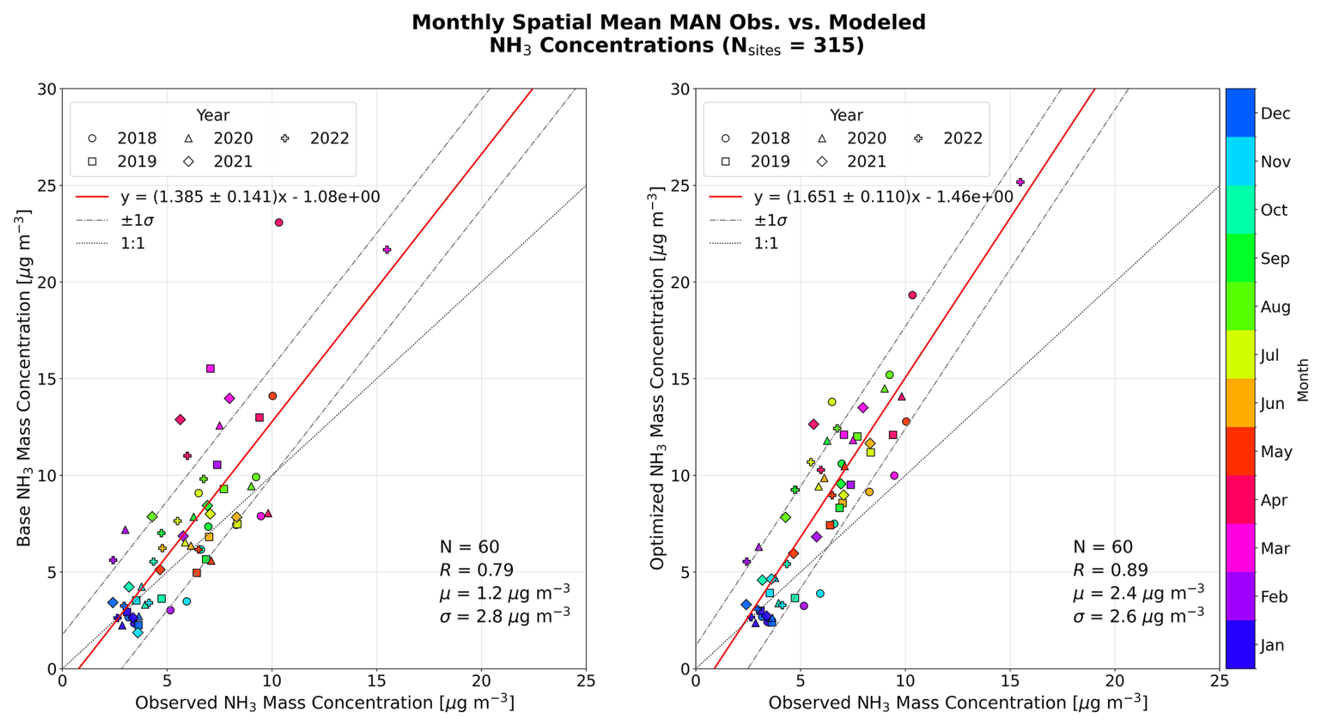
Figure 16Scatter plot of monthly spatial means of (left) base LOTOS-EUROS NH3, and (right) LOTOS-EUROS LETKF optimized NH3 vs. MAN observed NH3 surface concentrations for the period of January 2018–December 2022. Each data-point represents the mean calculated across all MAN sites for a given month, and are colored corresponding to the month while the marker style indicates the year. Uncertainty estimates for the reported statistics are provided in Table 2 and Appendix Table C1; paired bootstrap confidence intervals for optimized-minus-base changes are provided in Appendix Table C2.
These results indicate that the LETKF-optimized simulation better captures the large-scale spatial variability sampled by the MAN network, but that this improved spatial coherence does not correspond to an overall reduction in model error for the full MAN dataset. Instead, the optimized simulation increases the positive offset relative to MAN observations. This contrasts with the LML surface NH3 comparison, where the assimilation significantly reduced the negative bias and brought the regression slope closer to unity. The different behavior of the full MAN network is consistent with the representativeness interpretation discussed above: many MAN sites are located in Natura 2000 areas, often in sheltered or forested environments where local NH3 concentrations are lower than the surrounding landscape-scale concentrations represented by the 7 km×7 km model grid and by the satellite footprints used in the assimilation. Supporting visual comparisons using individual-site MAN monthly values and national monthly mean time series (Appendix Figs. B1 and B2) show a similar qualitative pattern to the full MAN-network comparison, with the optimized run better reproducing broad interannual variability but maintaining a high bias, particularly during the summer months of 2020 and 2022, the years with the strongest emission adjustments (see Fig. 2).
To further assess the spatial representativity of the MAN network and to enable a more direct comparison with the LML results, we also evaluated the six MAN calibration sensors co-located with LML sites against the base and optimized LETKF simulations. These six sensors are not part of the standard MAN dataset, but are used for the monthly calibration of the remaining 309 MAN sites, as described by Noordijk et al. (2020). A spatial-mean scatterplot for these six sensors is provided in Appendix Fig. B3, and the associated statistics are summarized in Table 2. In contrast to the full MAN network, the co-located MAN sensors show behavior consistent with the LML analysis. The mean bias is significantly reduced from to µg m−3 after assimilation ( µg m−3, 95 % CI: +0.85–+2.01 µg m−3). The spatial correlation also improves significantly from R=0.662 [0.490, 0.784] to R=0.761 [0.629, 0.851] (, 95 % CI: +0.011–+0.191), and the regression slope increases from 0.666±0.099 to 0.831±0.093 (, 95 % CI: +0.012–+0.325). The spread of the model–observation differences decreases from 3.57±0.33 to 3.15±0.29 µg m−3, although this change is not statistically significant. The much better agreement obtained for the co-located MAN calibration sensors indicates that the broader positive bias in the full MAN network is dominated primarily by representativeness differences rather than by a uniform model overestimation across all MAN locations. In other words, when the MAN comparison is restricted to more open, regionally representative sites similar to the LML locations, the optimized simulation shows statistically robust improvements in bias, slope, and spatial correlation. Part of this contrast may stem from measurement uncertainties in the passive Gradko samplers, but representativeness effects are expected to dominate. The LML stations and the satellite footprints sample air masses that are more representative of the broader agricultural landscape, whereas most MAN sites are located within Natura 2000 areas, frequently in or near forested environments where canopy shielding and strong local heterogeneity depress NH3 concentrations relative to the surrounding terrain. These sheltered conditions are highly localized and not captured by the coarse spatial scales of the regional model (7 km×7 km) or the 12–14 km nadir footprint of the satellite retrievals. As a result, the MAN measurements at these locations tend to reflect sub-grid processes rather than the landscape-average conditions that the model and satellite products are designed to represent. Remaining differences may also relate to how canopy deposition or near-surface mixing is expressed at these fine spatial scales, rather than broad model biases.
Overall, the MAN comparisons reaffirm that the LETKF enhances the spatial coherence of the NH3 fields and performs consistently when evaluated against regionally representative measurements such as the LML sites. The discrepancies observed at many MAN locations primarily reflect representativeness limitations inherent in comparing coarse-scale model and satellite products with low-temporal-resolution passive samplers situated in highly heterogeneous environments. Reducing these mismatches will likely require finer-scale process representation and more explicit treatment of land-cover–dependent effects in future assimilation studies.
This study demonstrates that assimilating NH3 and NO2 satellite observations into the LOTOS-EUROS model using the LETKF framework substantially improves the representation of reactive nitrogen dynamics over the Netherlands. By co-assimilating IASI, CrIS, and TROPOMI retrievals over 2018–2022, the system produced optimized emissions, deposition, and concentration fields. The optimized emission fields showed consistent spatial structures across years, with persistent increases in the southern and eastern Netherlands, and exhibited notable temporal shifts such as a reduced springtime emission peak and enhanced summertime emissions. These patterns are broadly consistent with recent observational and modeling studies evaluating NH3 emissions over the region (Ge et al., 2020; Van Der Graaf et al., 2022; Ding et al., 2024).
Validation against independent LML surface observations at six sites showed a statistically robust reduction in mean bias, from approximately −2.0 to −1.0 µg m−3, while changes in correlation were positive but more modest. Assimilation also improved the representation of diurnal cycles, reducing systematic underestimation and bringing simulated amplitudes closer to observations, although some residual site-specific variability remained. Comparisons with dissolved in precipitation provided a complementary downstream evaluation, showing statistically significant improvements in temporal correlation, temporal bias, temporal spread, and in the spatial correlation and spread of wet deposition differences, while the monthly spatial mean-bias change was more modest and not statistically significant. Sensitivity tests for 2020 indicated that the multi-satellite configuration performed best overall, with joint assimilation of IASI and CrIS NH3 and TROPOMI NO2 producing the lowest biases relative to LML.
Comparisons with monthly MAN observations showed a statistically significant improvement in spatial correlation after assimilation, from R=0.79 to R=0.89, but also a statistically significant increase in positive bias, from +1.2 to +2.4 µg m−3, for the full MAN network. These biases primarily reflect representativeness differences: many MAN sites are located within Natura 2000 areas, often in forested or sheltered environments where canopy effects and fine-scale heterogeneity suppress local NH3 levels relative to the surrounding agricultural landscape. Such localized variability is not resolved at the model grid scale or by satellite footprints, leading to systematic overestimation when landscape-scale fields are evaluated against sheltered MAN locations.
In contrast, the MAN calibration sensors co-located at six LML stations showed statistically robust improvements in bias, slope, and spatial correlation. At these sites, the pre-assimilation mean bias of −2.4 µg m−3 improved to −1.0 µg m−3, the regression slope increased from 0.67 to 0.83, and the spatial correlation increased from R=0.66 to R=0.76. These results support the interpretation that the broader MAN bias is primarily driven by representativeness differences. Together, the LML and MAN comparisons highlight both the strengthened large-scale spatial and temporal structure of NH3 after assimilation and the ongoing challenges of reconciling coarse-resolution model and satellite fields with passive samplers located in highly heterogeneous environments. Because the present LETKF setup optimizes total NH3 emissions rather than sector-resolved source contributions, the spatial emission adjustments shown here cannot be attributed robustly to individual source types. Further progress may be enabled by adopting a label-based Kalman filtering approach. The labeling functionality introduced in LOTOS-EUROS v2.3 could be extended to the LETKF, allowing sector-specific emission optimization and supporting finer-scale improvements.
The results also underscore the importance of satellite observation density, particularly for NH3. The year 2020, characterized by the highest availability of CrIS and IASI retrievals, showed the largest emission and concentration adjustments. The recent launch of MTG-IRS on the MTG-S1 platform (1 July 2025) presents a major opportunity: its expected half-hourly 4 km×4 km NH3 retrieval capability could provide unprecedented spatial and temporal coverage over Europe, enabling improved constraints on diurnal variability, better characterization of emission events, and more rigorous evaluation of emission inventories. A dedicated NH3 assimilation study using MTG-IRS is recommended once data become available.
In addition to these advancements, several refinements warrant further investigation. These include improving the representativeness between model and surface observations, enhancing the treatment of diurnal variability across source sectors, and conducting a full system simulation experiment (SSE) to rigorously evaluate LETKF performance.
Overall, these findings highlight the essential role of satellite constraints in advancing chemical transport modeling and nitrogen budget estimation. Co-assimilating complementary satellite instruments provides a pathway toward more accurate and internally consistent representations of reactive nitrogen, strengthening our ability to constrain emissions, evaluate inventories, and assess deposition at regional to national scales. The demonstrated improvements offer a strong foundation for exploiting emerging missions such as MTG-IRS, enabling continued progress toward capturing fine-scale processes and further improving assimilation performance in future studies.
A1 Vredepeel-Vredeweg hourly NH3 timeseries
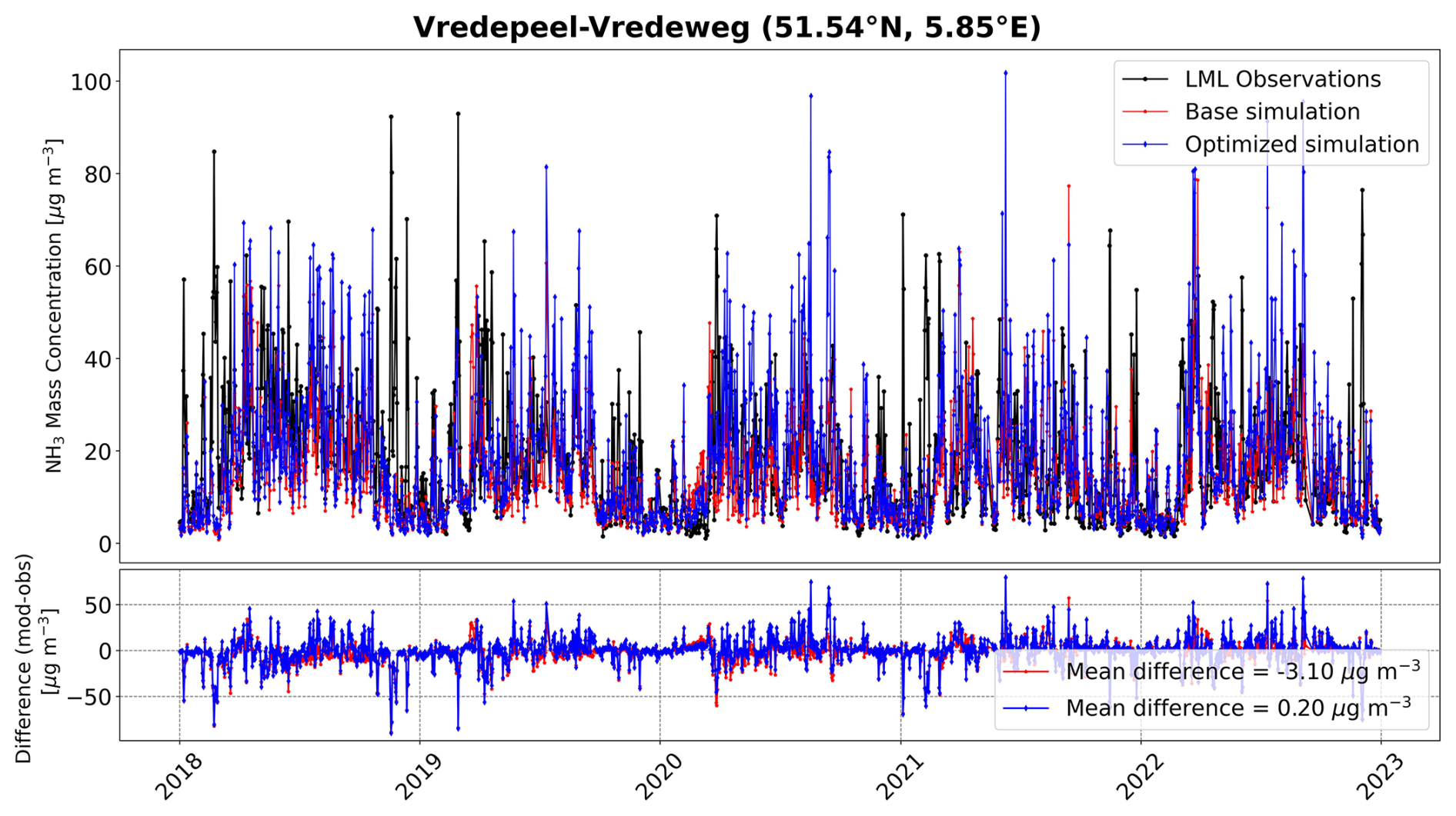
Figure A1Timeseries of hourly NH3 surface concentration values at the Vredepeel-Vredeweg LML site from (black) the observations, (red) the base LOTOS-EUROS simulation, and (blue) the LETKF-optimized simulation.
A2 LML comparisons for 2020 with base model simulation
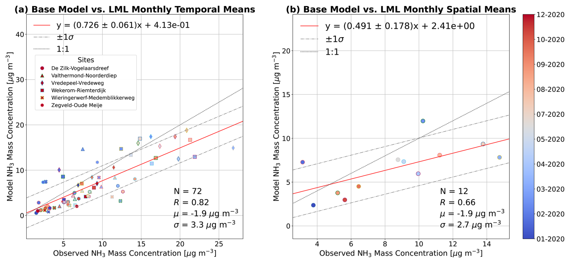
Figure A2Scatter plot of (a) monthly temporal means of LOTOS-EUROS simulated NH3 vs. LML observed NH3 surface concentrations, and (b) monthly spatial means of LOTOS-EUROS simulated NH3 vs. LML observed NH3 surface concentrations for the period of January–December 2020. Uncertainty estimates for the reported statistics are provided in Appendix Table C5.
B1 Monthly mean scatter plot pre- and post-assimilation
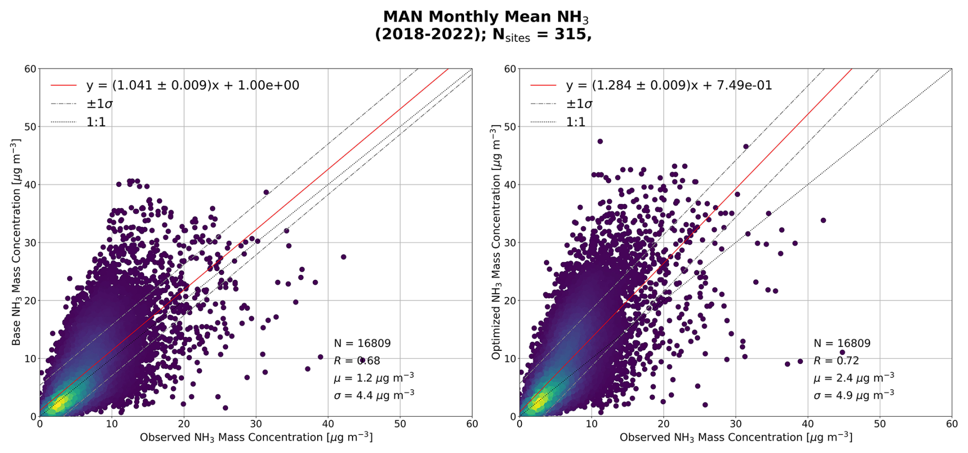
Figure B1Scatter plot comparing monthly means of observed MAN NH3 mass concentrations with (left) base LOTOS-EUROS surface NH3 mass concentration, and (right) LOTOS-EUROS LETKF optimized NH3 mass concentration. Each data-point represents a mean at a single MAN site. Uncertainty estimates for the reported statistics and paired bootstrap confidence intervals for optimized-minus-base changes are provided in Appendix Tables C1 and C2.
B2 Monthly mean timeseries
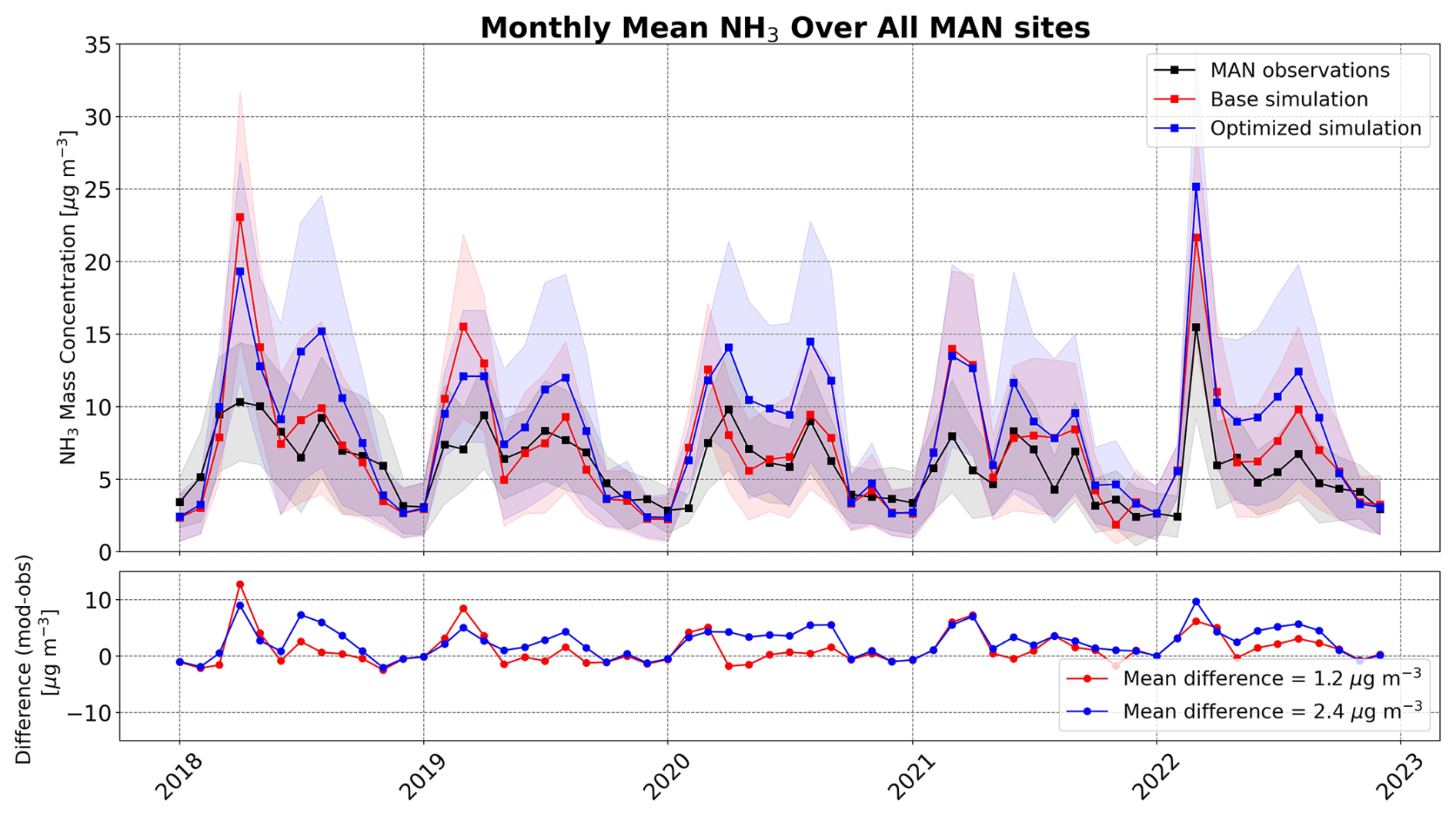
Figure B2Time-series of monthly mean NH3 surface mass concentrations and differences calculated across all MAN sites during 2018–2022. The shaded regions indicate the standard deviations of the monthly means. The mean differences shown in the monthly mean time series correspond to the same monthly spatial-mean comparisons summarized in Table 2 and Appendix Tables C1 and C2.
B3 MAN @ LML sites: spatial correlations
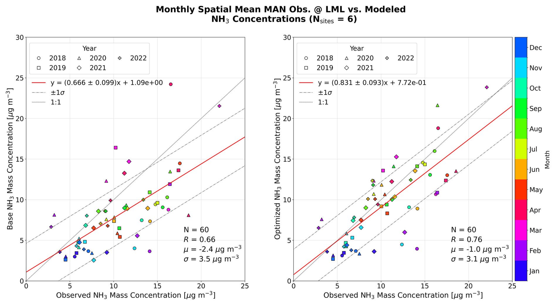
Figure B3Scatter plot of monthly spatial means of (left) base LOTOS-EUROS NH3, and (right) LOTOS-EUROS LETKF optimized NH3 vs. MAN observed NH3 surface concentrations at the locations of LML sites for the period of January 2018–December 2022. Each data-point represents the mean calculated across the 6 MAN calibration sensors located at the LML sites for a given month, and are colored corresponding to the month while the marker style indicates the year. Uncertainty estimates for the reported statistics are provided in Table 2 and Appendix Table C1; paired bootstrap confidence intervals for optimized-minus-base changes are provided in Appendix Table C2.
B4 MAN @ LML sites: monthly mean time-series
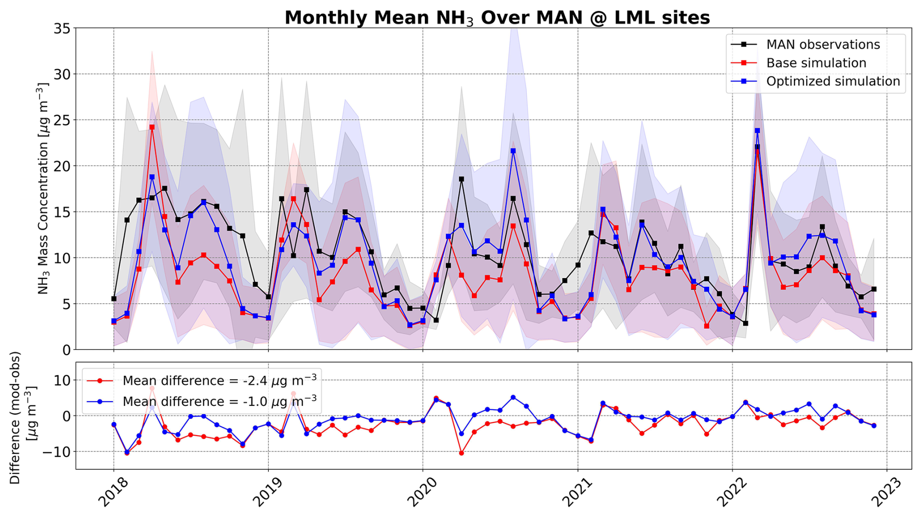
Figure B4Time-series of monthly mean NH3 surface mass concentrations and differences calculated across the 6 MAN calibration sensors located at the LML sites during 2018–2022. The shaded regions indicate the standard deviations of the monthly means. The mean differences shown in the monthly mean time series correspond to the same monthly spatial-mean comparisons summarized in Table 2 and Appendix Tables C1 and C2.
C1 Uncertainty estimates for surface NH3 comparisons
Table C1Full uncertainty estimates for model–observation comparison statistics. Values for the slope, mean bias (μ), and spread of model–observation differences (σ) are reported as estimate ± one standard error. Confidence intervals for R correspond to the 95 % interval obtained using the Fisher transformation. Units for μ and σ are µg m−3.
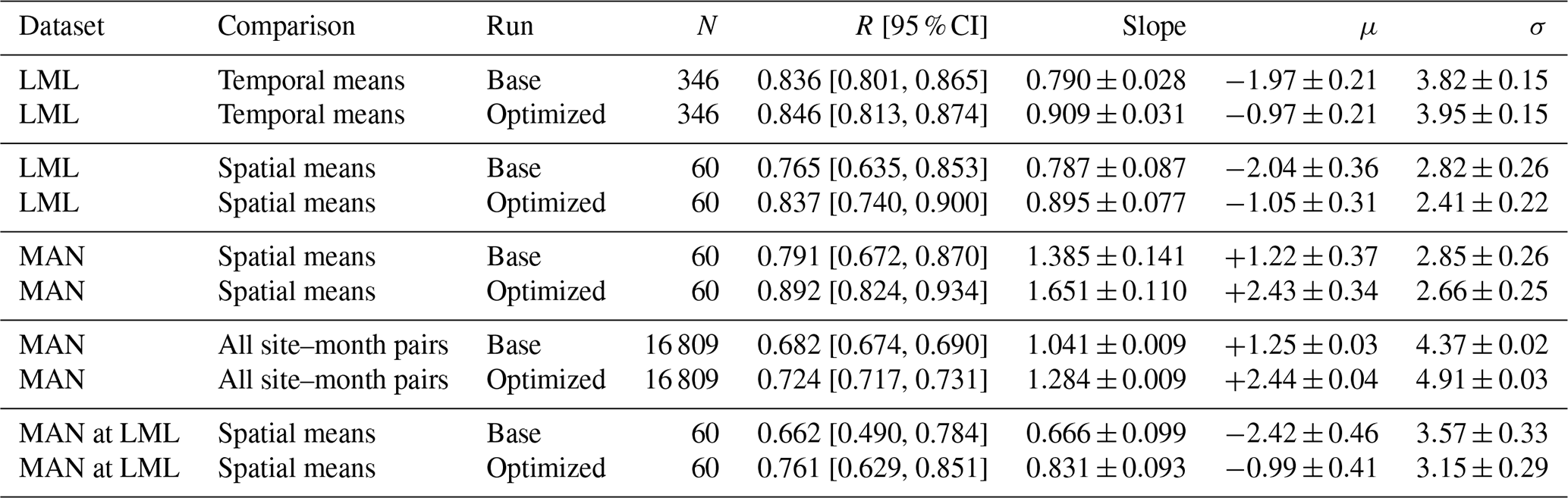
C2 Bootstrap assessment of optimized-minus-base changes for surface NH3 comparisons
Table C2Paired bootstrap estimates of optimized-minus-base changes in model–observation statistics. For each case, bootstrapping was performed with 10 000 bootstrap resamples. Confidence intervals represent 95 % bootstrap intervals. Statistically significant changes are those for which the confidence interval does not include zero. Units for Δμ and Δσ are µg m−3.

C3 Uncertainty estimates for wet deposition comparisons
Table C3Uncertainty estimates for wet deposition model–observation comparison statistics. Values for the slope, mean bias (μ), and spread of model–observation differences (σ) are reported as estimate ± one standard error. Confidence intervals for R correspond to the 95 % interval obtained using the Fisher transformation. Units for μ and σ are .

C4 Bootstrap assessment of optimized-minus-base changes for wet deposition comparisons
Table C4Paired bootstrap estimates of optimized-minus-base changes in wet deposition model–observation statistics. For each case, bootstrapping was performed with 10 000 bootstrap resamples. Confidence intervals represent 95 % bootstrap intervals. Statistically significant changes are those for which the confidence interval does not include zero. Units for Δμ and Δσ are .

C5 Uncertainty estimates for satellite-subset sensitivity experiments
Table C5Uncertainty estimates for the 2020 satellite-subset sensitivity experiments evaluated against LML NH3 surface observations. Values for the slope, mean bias (μ), and spread of model–observation differences (σ) are reported as estimate ± one standard error. Confidence intervals for R correspond to the 95 % interval obtained using the Fisher transformation. Units for μ and σ are µg m−3.
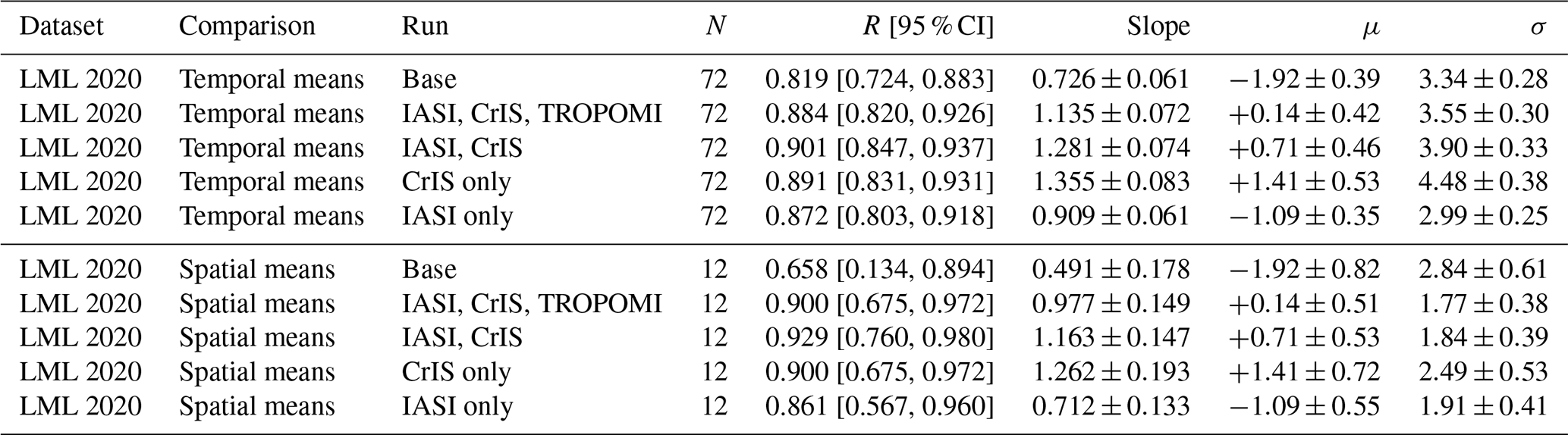
The use of the LOTOS-EUROS open-source version is regulated via registration. The open-source version of the model can be obtained from https://airqualitymodeling.tno.nl/lotos-euros/open-source-version/ (last access: 6 July 2026). Access to the LOTOS-EUROS LETKF can be provided upon formal request to the authors. The CAMS Satellite Operator (CSO) was used in this work and is an open-access tool developed at TNO and implemented to facilitate fast intercomparisons between modelled and satellite concentrations. CSO can be downloaded from: https://ci.tno.nl/gitlab/cams/cso (last access: 6 July 2026).
The CrIS NH3 v1.6.4 data from SNPP and NOAA-20 created by Environment and Climate Change Canada are currently publicly available upon request (mark.shephard@canada.ca). The IASI-NH3 v4 ANNI datasets (Clarisse et al., 2023) are available from the AERIS data infrastructure (https://iasi.aeris-data.fr/nh3/, last access: 26 August 2025). The TROPOMI NO2 version 2.4 data (van Geffen et al., 2022) are available on the Copernicus website (https://dataspace.copernicus.eu/, last access: 26 August 2025). The NH3 concentration and wet deposition data from the LML network are available on the RIVM website (https://data.rivm.nl/data/luchtmeetnet/, last access: 26 August 2025; LML, 2025). The monthly NH3 surface data from the MAN network are available at https://man.rivm.nl (last access: 26 August 2025; MAN, 2025) . Map data copyrighted OpenStreetMap contributors and available from https://www.openstreetmap.org/ (last access: 6 July 2026).
TW prepared the manuscript with contributions from all authors. TW, ED, and MS designed the experiment and provided scientific guidance during the project. AS developed the LOTOS-EUROS code and provided assistance with performing the assimilation runs. MWS, PC, MVD, LC, and HE developed the satellite retrievals and provided the data. RWK and SvdG provided the LML and MAN data and provided feedback on the analysis of these datasets. TW performed the formal analysis and presentation of the results.
The contact author has declared that none of the authors has any competing interests.
Publisher's note: Copernicus Publications remains neutral with regard to jurisdictional claims made in the text, published maps, institutional affiliations, or any other geographical representation in this paper. The authors bear the ultimate responsibility for providing appropriate place names. Views expressed in the text are those of the authors and do not necessarily reflect the views of the publisher.
Lieven Clarisse is a senior research associate supported by the Belgian F.R.S.-FNRS. Generative AI tools were used in the drafting and editing process of this manuscript.
This study was funded by the Dutch Ministry of Agriculture, Fisheries, Food Security and Nature (LVVN), within the framework of the National Nitrogen Knowledge Programme (NKS), project NKS-SAGEN, on satellite observations and ensemble modeling.
This paper was edited by Eric Kort and reviewed by two anonymous referees.
Berkhout, A. J. C., Swart, D. P. J., Volten, H., Gast, L. F. L., Haaima, M., Verboom, H., Stefess, G., Hafkenscheid, T., and Hoogerbrugge, R.: Replacing the AMOR with the miniDOAS in the ammonia monitoring network in the Netherlands, Atmos. Meas. Tech., 10, 4099–4120, https://doi.org/10.5194/amt-10-4099-2017, 2017. a, b
Bessagnet, B., Pirovano, G., Mircea, M., Cuvelier, C., Aulinger, A., Calori, G., Ciarelli, G., Manders, A., Stern, R., Tsyro, S., García Vivanco, M., Thunis, P., Pay, M.-T., Colette, A., Couvidat, F., Meleux, F., Rouíl, L., Ung, A., Aksoyoglu, S., Baldasano, J. M., Bieser, J., Briganti, G., Cappelletti, A., D'Isidoro, M., Finardi, S., Kranenburg, R., Silibello, C., Carnevale, C., Aas, W., Dupont, J.-C., Fagerli, H., Gonzalez, L., Menut, L., Prévôt, A. S. H., Roberts, P., and White, L.: Presentation of the EURODELTA III intercomparison exercise – evaluation of the chemistry transport models' performance on criteria pollutants and joint analysis with meteorology, Atmos. Chem. Phys., 16, 12667–12701, https://doi.org/10.5194/acp-16-12667-2016, 2016. a
Chan, K. L., Wiegner, M., van Geffen, J., De Smedt, I., Alberti, C., Cheng, Z., Ye, S., and Wenig, M.: MAX-DOAS measurements of tropospheric NO2 and HCHO in Munich and the comparison to OMI and TROPOMI satellite observations, Atmos. Meas. Tech., 13, 4499–4520, https://doi.org/10.5194/amt-13-4499-2020, 2020. a
Chen, Z., Jacob, D. J., Gautam, R., Omara, M., Stavins, R. N., Stowe, R. C., Nesser, H., Sulprizio, M. P., Lorente, A., Varon, D. J., Lu, X., Shen, L., Qu, Z., Pendergrass, D. C., and Hancock, S.: Satellite quantification of methane emissions and oil–gas methane intensities from individual countries in the Middle East and North Africa: implications for climate action, Atmos. Chem. Phys., 23, 5945–5967, https://doi.org/10.5194/acp-23-5945-2023, 2023. a, b
Clarisse, L., Franco, B., Van Damme, M., Di Gioacchino, T., Hadji-Lazaro, J., Whitburn, S., Noppen, L., Hurtmans, D., Clerbaux, C., and Coheur, P.: The IASI NH3 version 4 product: averaging kernels and improved consistency, Atmos. Meas. Tech., 16, 5009–5028, https://doi.org/10.5194/amt-16-5009-2023, 2023. a, b, c
Clerbaux, C., Boynard, A., Clarisse, L., George, M., Hadji-Lazaro, J., Herbin, H., Hurtmans, D., Pommier, M., Razavi, A., Turquety, S., Wespes, C., and Coheur, P.-F.: Monitoring of atmospheric composition using the thermal infrared IASI/MetOp sounder, Atmos. Chem. Phys., 9, 6041–6054, https://doi.org/10.5194/acp-9-6041-2009, 2009. a
Colette, A., Andersson, C., Manders, A., Mar, K., Mircea, M., Pay, M.-T., Raffort, V., Tsyro, S., Cuvelier, C., Adani, M., Bessagnet, B., Bergström, R., Briganti, G., Butler, T., Cappelletti, A., Couvidat, F., D'Isidoro, M., Doumbia, T., Fagerli, H., Granier, C., Heyes, C., Klimont, Z., Ojha, N., Otero, N., Schaap, M., Sindelarova, K., Stegehuis, A. I., Roustan, Y., Vautard, R., van Meijgaard, E., Vivanco, M. G., and Wind, P.: EURODELTA-Trends, a multi-model experiment of air quality hindcast in Europe over 1990–2010, Geosci. Model Dev., 10, 3255–3276, https://doi.org/10.5194/gmd-10-3255-2017, 2017. a
Colette, A., Collin, G., Besson, F., Blot, E., Guidard, V., Meleux, F., Royer, A., Petiot, V., Miller, C., Fermond, O., Jeant, A., Adani, M., Arteta, J., Benedictow, A., Bergström, R., Bowdalo, D., Brandt, J., Briganti, G., Carvalho, A. C., Christensen, J. H., Couvidat, F., D'Elia, I., D'Isidoro, M., Denier van der Gon, H., Descombes, G., Di Tomaso, E., Douros, J., Escribano, J., Eskes, H., Fagerli, H., Fatahi, Y., Flemming, J., Friese, E., Frohn, L., Gauss, M., Geels, C., Guarnieri, G., Guevara, M., Guion, A., Guth, J., Hänninen, R., Hansen, K., Im, U., Janssen, R., Jeoffrion, M., Joly, M., Jones, L., Jorba, O., Kadantsev, E., Kahnert, M., Kaminski, J. W., Kouznetsov, R., Kranenburg, R., Kuenen, J., Lange, A. C., Langner, J., Lannuque, V., Macchia, F., Manders, A., Mircea, M., Nyiri, A., Olid, M., Pérez García-Pando, C., Palamarchuk, Y., Piersanti, A., Raux, B., Razinger, M., Robertson, L., Segers, A., Schaap, M., Siljamo, P., Simpson, D., Sofiev, M., Stangel, A., Struzewska, J., Tena, C., Timmermans, R., Tsikerdekis, T., Tsyro, S., Tyuryakov, S., Ung, A., Uppstu, A., Valdebenito, A., van Velthoven, P., Vitali, L., Ye, Z., Peuch, V.-H., and Rouíl, L.: Copernicus Atmosphere Monitoring Service – Regional Air Quality Production System v1.0, Geosci. Model Dev., 18, 6835–6883, https://doi.org/10.5194/gmd-18-6835-2025, 2025. a, b
Crutzen, P. J.: The role of NO and NO2 in the chemistry of the troposphere and stratosphere, Annu. Rev. Earth Pl. Sc., 7, 443–472, https://doi.org/10.1146/annurev.ea.07.050179.002303, 1979. a
Dammers, E., Palm, M., Van Damme, M., Vigouroux, C., Smale, D., Conway, S., Toon, G. C., Jones, N., Nussbaumer, E., Warneke, T., Petri, C., Clarisse, L., Clerbaux, C., Hermans, C., Lutsch, E., Strong, K., Hannigan, J. W., Nakajima, H., Morino, I., Herrera, B., Stremme, W., Grutter, M., Schaap, M., Wichink Kruit, R. J., Notholt, J., Coheur, P.-F., and Erisman, J. W.: An evaluation of IASI−NH3 with ground-based Fourier transform infrared spectroscopy measurements, Atmos. Chem. Phys., 16, 10351–10368, https://doi.org/10.5194/acp-16-10351-2016, 2016. a, b
Dammers, E., Shephard, M. W., Palm, M., Cady-Pereira, K., Capps, S., Lutsch, E., Strong, K., Hannigan, J. W., Ortega, I., Toon, G. C., Stremme, W., Grutter, M., Jones, N., Smale, D., Siemons, J., Hrpcek, K., Tremblay, D., Schaap, M., Notholt, J., and Erisman, J. W.: Validation of the CrIS fast physical NH3 retrieval with ground-based FTIR, Atmos. Meas. Tech., 10, 2645–2667, https://doi.org/10.5194/amt-10-2645-2017, 2017. a, b
Ding, J., van der A, R., Eskes, H., Dammers, E., Shephard, M., Wichink Kruit, R., Guevara, M., and Tarrason, L.: Ammonia emission estimates using CrIS satellite observations over Europe, Atmos. Chem. Phys., 24, 10583–10599, https://doi.org/10.5194/acp-24-10583-2024, 2024. a, b
Douros, J., Eskes, H., van Geffen, J., Boersma, K. F., Compernolle, S., Pinardi, G., Blechschmidt, A.-M., Peuch, V.-H., Colette, A., and Veefkind, P.: Comparing Sentinel-5P TROPOMI NO2 column observations with the CAMS regional air quality ensemble, Geosci. Model Dev., 16, 509–534, https://doi.org/10.5194/gmd-16-509-2023, 2023. a
Elskamp, H.: National Air Quality Monitoring Network. Technical description, Report 228702017, http://hdl.handle.net/10029/259431 (last access: 6 July 2026), 1989. a
Elzakker, B. and Buijsman, E.: Meetactiviteiten in 1999 in het Landelijk Meetnet Luchtkwaliteit, Report 723101032, https://www.rivm.nl/bibliotheek/rapporten/729999002.pdf (last access: 6 July 2026), 1999. a
Erisman, J. W., Sutton, M. A., Galloway, J., Zbigniew, K., and Winiwarter, W.: How a century of ammonia synthesis changed the world, Nat. Geosci., 1, 636–639, https://doi.org/10.1038/ngeo325, 2008. a
Erisman, J. W., van Grinsven, H., Grizzetti, B., Bouraoui, F., Powlson, D., Sutton, M. A., Bleeker, A., and Reis, S.: The European Nitrogen Problem in a Global Perspective, Cambridge University Press, https://doi.org/10.1017/cbo9780511976988.005, 9–31, 2011. a, b, c
Eskes, H., van Geffen, J., Boersma, K., Eichmann, K.-U., Apituley, A., Pedergnana, M., Sneep, M., Veefkind, J. P., and Loyola, D.: Sentinel-5 precursor/TROPOMI Level 2 Product User Manual Nitrogendioxide, Tech. Rep. S5P-KNMI-L2-0021-MA, Koninklijk Nederlands Meteorologisch Instituut (KNMI), issue 4.3.0, processor version 2.7.1, CI-7570-PUM, date 4 April 2024, https://doi.org/10.5270/S5P-9bnp8q8, 2024. a
Eum, K. D., Honda, T. J., Wang, B., Kazemiparkouhi, F., Manjourides, J., Pun, V. C., Pavlu, V., and Suh, H.: Long-term nitrogen dioxide exposure and cause-specific mortality in the U.S. Medicare population, Environ. Res., 207, https://doi.org/10.1016/j.envres.2021.112154, 2022. a
Evensen, G.: The ensemble Kalman filter: theoretical formulation and practical implementation, Ocean Dynam., 53, 343–367, https://doi.org/10.1007/s10236-003-0036-9, 2003. a
Finlayson-Pitts, B. J. and Pitts, J. N.: Chemistry of the Upper and Lower Atmosphere: Theory, Experiments, and Applications, Academic Press, San Diego, ISBN 978-0-12-257060-5, https://doi.org/10.1016/B978-0-12-257060-5.X5000-X, 2000. a
Galloway, J. N., Townsend, A. R., Erisman, J. W., Bekunda, M., Cai, Z., Freney, J. R., Martinelli, L. A., Seitzinger, S. P., and Sutton, M. A.: Transformation of the nitrogen cycle: recent trends, questions, and potential solutions, Science, 320, 889–892, https://doi.org/10.1126/science.1136674, 2008. a, b
Ge, X., Schaap, M., Kranenburg, R., Segers, A., Reinds, G. J., Kros, H., and de Vries, W.: Modeling atmospheric ammonia using agricultural emissions with improved spatial variability and temporal dynamics, Atmos. Chem. Phys., 20, 16055–16087, https://doi.org/10.5194/acp-20-16055-2020, 2020. a, b, c, d, e
Ge, X., Schaap, M., Dammers, E., Shephard, M., and de Vries, W.: Impact of interannual weather variation on ammonia emissions and concentrations in Germany, Agr. Forest Meteorol., 334, https://doi.org/10.1016/j.agrformet.2023.109432, 2023. a, b
Griffin, D., Zhao, X., McLinden, C. A., Boersma, F., Bourassa, A., Dammers, E., Degenstein, D., Eskes, H., Fehr, L., Fioletov, V., Hayden, K., Kharol, S. K., Li, S.-M., Makar, P., Martin, R. V., Mihele, C., Mittermeier, R. L., Krotkov, N., Sneep, M., Lamsal, L. N., Linden, M. t., Geffen, J. v., Veefkind, P., and Wolde, M.: High-resolution mapping of nitrogen dioxide with TROPOMI: first results and validation over the Canadian oil sands, Geophys. Res. Lett., 46, 1049–1060, https://doi.org/10.1029/2018GL081095, 2019. a
Guo, X., Wang, R., Pan, D., Zondlo, M. A., Clarisse, L., Damme, M. V., Whitburn, S., Coheur, P. F., Clerbaux, C., Franco, B., Golston, L. M., Wendt, L., Sun, K., Tao, L., Miller, D., Mikoviny, T., Müller, M., Wisthaler, A., Tevlin, A. G., Murphy, J. G., Nowak, J. B., Roscioli, J. R., Volkamer, R., Kille, N., Neuman, J. A., Eilerman, S. J., Crawford, J. H., Yacovitch, T. I., Barrick, J. D., and Scarino, A. J.: Validation of IASI satellite ammonia observations at the pixel scale using in situ vertical profiles, J. Geophys. Res.-Atmos., 126, https://doi.org/10.1029/2020JD033475, 2021. a
Gyldenkærne, S., Skjøth, C. A., Hertel, O., and Ellermann, T.: A dynamical ammonia emission parameterization for use in air pollution models, J. Geophys. Res.-Atmos., 110, 1–14, https://doi.org/10.1029/2004JD005459, 2005. a
Herrera, B., Bezanilla, A., Blumenstock, T., Dammers, E., Hase, F., Clarisse, L., Magaldi, A., Rivera, C., Stremme, W., Strong, K., Viatte, C., Van Damme, M., and Grutter, M.: Measurement report: Evolution and distribution of NH3 over Mexico City from ground-based and satellite infrared spectroscopic measurements, Atmos. Chem. Phys., 22, 14119–14132, https://doi.org/10.5194/acp-22-14119-2022, 2022. a
Hunt, B. R., Kostelich, E. J., and Szunyogh, I.: Efficient data assimilation for spatiotemporal chaos: a local ensemble transform Kalman filter, Physica D, 230, 112–126, https://doi.org/10.1016/j.physd.2006.11.008, 2007. a
Iturbide-Sanchez, F., Strow, L., Tobin, D., Chen, Y., Tremblay, D., Knuteson, R. O., Johnson, D. G., Buttles, C., Suwinski, L., Thomas, B. P., Rivera, A. R., Lynch, E., Zhang, K., Wang, Z., Porter, W. D., Jin, X., Predina, J. P., Eresmaa, R. I., Collard, A., Ruston, B., Jung, J. A., Barnet, C. D., Beierle, P. J., Yan, B., Mooney, D., and Revercomb, H.: Recalibration and assessment of the SNPP CrIS instrument: a successful history of restoration after midwave infrared band anomaly, IEEE T. Geosci. Remote, 60, https://doi.org/10.1109/TGRS.2021.3112400, 2022. a
Jonson, J. E., Borken-Kleefeld, J., Simpson, D., Nyíri, A., Posch, M., and Heyes, C.: Impact of excess NOx emissions from diesel cars on air quality, public health and eutrophication in Europe, Environ. Res. Lett., 12, https://doi.org/10.1088/1748-9326/aa8850, 2017. a
Judd, L. M., Al-Saadi, J. A., Szykman, J. J., Valin, L. C., Janz, S. J., Kowalewski, M. G., Eskes, H. J., Veefkind, J. P., Cede, A., Mueller, M., Gebetsberger, M., Swap, R., Pierce, R. B., Nowlan, C. R., Abad, G. G., Nehrir, A., and Williams, D.: Evaluating Sentinel-5P TROPOMI tropospheric NO2 column densities with airborne and Pandora spectrometers near New York City and Long Island Sound, Atmos. Meas. Tech., 13, 6113–6140, https://doi.org/10.5194/amt-13-6113-2020, 2020. a
Kuenen, J., Dellaert, S., Visschedijk, A., Jalkanen, J.-P., Super, I., and Denier van der Gon, H.: CAMS-REG-v4: a state-of-the-art high-resolution European emission inventory for air quality modelling, Earth Syst. Sci. Data, 14, 491–515, https://doi.org/10.5194/essd-14-491-2022, 2022. a, b
Kutzner, R. D., Cuesta, J., Chelin, P., Petit, J.-E., Ray, M., Landsheere, X., Tournadre, B., Dupont, J.-C., Rosso, A., Hase, F., Orphal, J., and Beekmann, M.: Diurnal evolution of total column and surface atmospheric ammonia in the megacity of Paris, France, during an intense springtime pollution episode, Atmos. Chem. Phys., 21, 12091–12111, https://doi.org/10.5194/acp-21-12091-2021, 2021. a
Lambert, J.-C., Keppens, A., Compernolle, S., Eichmann, K.-U., de Graaf, M., Hubert, D., Langerock, B., Ludewig, A., Sha, M. K., Verhoelst, T., Wagner, T., Ahn, C., Argyrouli, A., Balis, D., Chan, K. L., Coldewey-Egbers, M., De Smedt, I., Eskes, H., Fjæraa, A. M., Garane, K., Gleason, J. F., Goutail, F., Granville, J., Hedelt, P., Heue, K.-P., Jaross, G., Kleipool, Q., Koukouli, M. L., Lutz, R., Martinez Velarte, M. C., Michailidis, K., Pseftogkas, A., Nanda, S., Niemeijer, S., Pazmiño, A., Pinardi, G., Richter, A., Rozemeijer, N., Sneep, M., Stein Zweers, D., Theys, N., Tilstra, G., Torres, O., Valks, P., van Geffen, J., Vigouroux, C., Wang, P., and Weber, M.: Quarterly Validation Report of the Copernicus Sentinel-5 Precursor Operational Data Products #24: April 2018–August 2024, S5P MPC Routine Operations Consolidated Validation Report Series Issue #24, Version 24.00.00, 16 September 2024, S5P Mission Performance Centre, https://mpc-vdaf.tropomi.eu/ProjectDir/reports//pdf/S5P-MPC-IASB-ROCVR-24.00.00_FINAL_signed.pdf (last access: 6 July 2026), 2024. a
Liu, S., Jørgensen, J. T., Ljungman, P., Pershagen, G., Bellander, T., Leander, K., Magnusson, P. K., Rizzuto, D., Hvidtfeldt, U. A., Raaschou-Nielsen, O., Wolf, K., Hoffmann, B., Brunekreef, B., Strak, M., Chen, J., Mehta, A., Atkinson, R. W., Bauwelinck, M., Varraso, R., Boutron-Ruault, M.-C., Brandt, J., Cesaroni, G., Forastiere, F., Fecht, D., Gulliver, J., Hertel, O., de Hoogh, K., Janssen, N. A., Katsouyanni, K., Ketzel, M., Klompmaker, J. O., Nagel, G., Oftedal, B., Peters, A., Tjønneland, A., Rodopoulou, S. P., Samoli, E., Kristoffersen, D. T., Sigsgaard, T., Stafoggia, M., Vienneau, D., Weinmayr, G., Hoek, G., and Andersen, Z. J.: Long-term exposure to low-level air pollution and incidence of asthma: the ELAPSE project, Eur. Respir. J., 57, 2003099, https://doi.org/10.1183/13993003.030992020, 2021. a
LML: Dutch Air Quality Monitoring, Rijksinstituut voor Volksgezondheid en Milieu [data set], https://data.rivm.nl/data/luchtmeetnet/ (last access: 6 July 2026), 2025. a
Lolkema, D. E., Noordijk, H., Stolk, A. P., Hoogerbrugge, R., van Zanten, M. C., and van Pul, W. A. J.: The Measuring Ammonia in Nature (MAN) network in the Netherlands, Biogeosciences, 12, 5133–5142, https://doi.org/10.5194/bg-12-5133-2015, 2015. a, b, c, d
Lopez-Restrepo, S., Yarce, A., Pinel, N., Quintero, O. L., Segers, A., and Heemink, A. W.: Forecasting PM10 and PM2.5 in the Aburrá Valley (Medellín, Colombia) via EnKF based data assimilation, Atmos. Environ., 232, https://doi.org/10.1016/j.atmosenv.2020.117507, 2020. a, b
Lô, S., Dohmen, W., Heederik, D., Weijers, E., van Schothorst, I., Bleeker, A., Vermeulen, R., and Hoek, G.: Spatial and temporal variability of atmospheric ammonia using a dense network in an area with livestock, residential and natural environments intertwined, Atmos. Environ., 360, https://doi.org/10.1016/j.atmosenv.2025.121394, 2025. a
MAN: Dutch Measuring Ammonia in Nature, Rijksinstituut voor Volksgezondheid en Milieu [data set], https://man.rivm.nl (last access: 6 July 2026), 2025. a
Manders, A. M. M., Builtjes, P. J. H., Curier, L., Denier van der Gon, H. A. C., Hendriks, C., Jonkers, S., Kranenburg, R., Kuenen, J. J. P., Segers, A. J., Timmermans, R. M. A., Visschedijk, A. J. H., Wichink Kruit, R. J., van Pul, W. A. J., Sauter, F. J., van der Swaluw, E., Swart, D. P. J., Douros, J., Eskes, H., van Meijgaard, E., van Ulft, B., van Velthoven, P., Banzhaf, S., Mues, A. C., Stern, R., Fu, G., Lu, S., Heemink, A., van Velzen, N., and Schaap, M.: Curriculum vitae of the LOTOS–EUROS (v2.0) chemistry transport model, Geosci. Model Dev., 10, 4145–4173, https://doi.org/10.5194/gmd-10-4145-2017, 2017. a, b, c
Moncet, J.-L., Uymin, G., Lipton, A. E., and Snell, H. E.: Infrared radiance modeling by optimal spectral sampling, J. Atmos. Sci., 65, 3917–3934, https://doi.org/10.1175/2008JAS2711.1, 2008. a
Noordijk, H., Braam, M., Rutledge-Jonker, S., Hoogerbrugge, R., Stolk, A. P., and van Pul, W. A.: Performance of the MAN ammonia monitoring network in the Netherlands, Atmos. Environ., 228, https://doi.org/10.1016/j.atmosenv.2020.117400, 2020. a, b, c, d
Ojeda-Castillo, V., Murillo-Tovar, M. A., Hernández-Mena, L., Saldarriaga-Noreña, H., Vargas-Amado, M. E., Herrera-López, E. J., and Díaz, J.: Tropospheric NO2: anthropogenic influence, global trends, satellite data, and machine learning application, Remote Sens.-Basel, 17, https://doi.org/10.3390/rs17010049, 2025. a
OpenStreetMap contributors: Planet dump, https://planet.osm.org (last access: 6 July 2026), 2017. a
Paulot, F., Jacob, D. J., Pinder, R. W., Bash, J. O., Travis, K., and Henze, D. K.: Ammonia emissions in the United States, European Union, and China derived by high-resolution inversion of ammonium wet deposition data: interpretation with a new agricultural emissions inventory (MASAGE_NH3), J. Geophys. Res.-Atmos., 119, 4343–4364, https://doi.org/10.1002/2013JD021130, 2014. a
Peuch, V.-H., Engelen, R., Rixen, M., Dee, D., Flemming, J., Suttie, M., Ades, M., Agustí-Panareda, A., Ananasso, C., Andersson, E., Armstrong, D., Barré, J., Bousserez, N., Dominguez, J. J., Garrigues, S., Inness, A., Jones, L., Kipling, Z., Letertre-Danczak, J., Parrington, M., Razinger, M., Ribas, R., Vermoote, S., Yang, X., Simmons, A., Garcés De Marcilla, J., and Thépaut, J.-N.: The Copernicus Atmosphere Monitoring Service: from research to operations, B. Am. Meteorol. Soc., 103, E2650–E2668, https://doi.org/10.1175/BAMS-D-21-0314.1, 2022. a
Pope, C. A. and Dockery, D. W.: Health effects of fine particulate air pollution: lines that connect, J. Air Waste Manage., 56, 709–742, https://doi.org/10.1080/10473289.2006.10464485, 2006. a
Pope, C. A., Ezzati, M., and Dockery, D. W.: Fine-particulate air pollution and life expectancy in the United States, New Engl. J. Med., 360, 376–386, https://doi.org/10.1056/nejmsa0805646, 2009. a
Rodgers, C. D.: Inverse Methods for Atmospheric Sounding: Theory and Practice, Vol. 2 of Series on Atmospheric, Oceanic and Planetary Physics, World Scientific, https://doi.org/10.1142/3171, 2000. a, b
Rodgers, C. D. and Connor, B. J.: Intercomparison of remote sounding instruments, J. Geophys. Res.-Atmos., 108, https://doi.org/10.1029/2002jd002299, 2003. a
Schaap, M., Timmermans, R. M., Roemer, M., Boersen, G., Builtjes, P. J., Sauter, F. J., Velders, G. J., Beck, J. P., and Sauter, P.: The LOTOS-EUROS model: description, validation and latest developments The LOTOS-EUROS model, Tech. rep., https://doi.org/10.1504/IJEP.2008.017106, 2008. a
Shephard, M. W. and Cady-Pereira, K. E.: Cross-track Infrared Sounder (CrIS) satellite observations of tropospheric ammonia, Atmos. Meas. Tech., 8, 1323–1336, https://doi.org/10.5194/amt-8-1323-2015, 2015. a
Shephard, M. W., Dammers, E., Cady-Pereira, K. E., Kharol, S. K., Thompson, J., Gainariu-Matz, Y., Zhang, J., McLinden, C. A., Kovachik, A., Moran, M., Bittman, S., Sioris, C. E., Griffin, D., Alvarado, M. J., Lonsdale, C., Savic-Jovcic, V., and Zheng, Q.: Ammonia measurements from space with the Cross-track Infrared Sounder: characteristics and applications, Atmos. Chem. Phys., 20, 2277–2302, https://doi.org/10.5194/acp-20-2277-2020, 2020. a
Shephard, M. W., Kharol, S. K., Dammers, E., Sioris, C. E., Bell, A., Jansen, R., Caron, J., Snel, R., Palombo, E., Cady-Pereira, K. E., McLinden, C. A., Lutsch, E., and Knuteson, R. O.: Infrared satellite detection limits for monitoring atmospheric ammonia, IEEE J. Sel. Top. Appl., 18, 10272–10291, https://doi.org/10.1109/JSTARS.2025.3557240, 2025. a
Shin, S., Kang, J. S., and Jo, Y.: The Local Ensemble Transform Kalman Filter (LETKF) with a global NWP model on the cubed sphere, Pure Appl. Geophys., 173, 2555–2570, https://doi.org/10.1007/s00024-016-1269-0, 2016. a, b, c, d, e
Sutton, M. A., Oenema, O., Erisman, J. W., Leip, A., van Grinsven, H., and Winiwarter, W.: Too much of a good thing, Nature, 472, 159–161, https://doi.org/10.1038/472159a, 2011. a, b
Søgaard, H. T., Sommer, S. G., Hutchings, N. J., Huijsmans, J. F. M., Bussink, D. W., and Nicholson, F.: Ammonia volatilization from field-applied animal slurry-the ALFAM model, Tech. rep., https://doi.org/10.1016/S1352-2310(02)00300-X, 2002. a
Timmermans, R., Segers, A., Curier, L., Abida, R., Attié, J.-L., El Amraoui, L., Eskes, H., de Haan, J., Kujanpæ, J., Lahoz, W., Oude Nijhuis, A., Quesada-Ruiz, S., Ricaud, P., Veefkind, P., and Schaap, M.: Impact of synthetic space-borne NO2 observations from the Sentinel-4 and Sentinel-5P missions on tropospheric NO2 analyses , Atmos. Chem. Phys., 19, 12811–12833, https://doi.org/10.5194/acp-19-12811-2019, 2019. a
Tsyro, S., Aas, W., Colette, A., Andersson, C., Bessagnet, B., Ciarelli, G., Couvidat, F., Cuvelier, K., Manders, A., Mar, K., Mircea, M., Otero, N., Pay, M.-T., Raffort, V., Roustan, Y., Theobald, M. R., Vivanco, M. G., Fagerli, H., Wind, P., Briganti, G., Cappelletti, A., D'Isidoro, M., and Adani, M.: Eurodelta multi-model simulated and observed particulate matter trends in Europe in the period of 1990–2010, Atmos. Chem. Phys., 22, 7207–7257, https://doi.org/10.5194/acp-22-7207-2022, 2022. a
Van Damme, M., Clarisse, L., Heald, C. L., Hurtmans, D., Ngadi, Y., Clerbaux, C., Dolman, A. J., Erisman, J. W., and Coheur, P. F.: Global distributions, time series and error characterization of atmospheric ammonia (NH3) from IASI satellite observations, Atmos. Chem. Phys., 14, 2905–2922, https://doi.org/10.5194/acp-14-2905-2014, 2014. a
Van Damme, M., Whitburn, S., Clarisse, L., Clerbaux, C., Hurtmans, D., and Coheur, P.-F.: Version 2 of the IASI NH3 neural network retrieval algorithm: near-real-time and reanalysed datasets, Atmos. Meas. Tech., 10, 4905–4914, https://doi.org/10.5194/amt-10-4905-2017, 2017. a, b
Van Damme, M., Clarisse, L., Stavrakou, T., Wichink Kruit, R., Sellekaerts, L., Viatte, C., Clerbaux, C., and Coheur, P. F.: On the weekly cycle of atmospheric ammonia over European agricultural hotspots, Sci. Rep.-UK, 12, https://doi.org/10.1038/s41598-022-15836-w, 2022. a
van der Graaf, S., Dammers, E., Segers, A., Kranenburg, R., Schaap, M., Shephard, M. W., and Erisman, J. W.: Data assimilation of CrIS NH3 satellite observations for improving spatiotemporal NH3 distributions in LOTOS-EUROS, Atmos. Chem. Phys., 22, 951–972, https://doi.org/10.5194/acp-22-951-2022, 2022. a, b, c, d, e, f, g, h, i
van Geffen, J., Eskes, H., Compernolle, S., Pinardi, G., Verhoelst, T., Lambert, J.-C., Sneep, M., ter Linden, M., Ludewig, A., Boersma, K. F., and Veefkind, J. P.: Sentinel-5P TROPOMI NO2 retrieval: impact of version v2.2 improvements and comparisons with OMI and ground-based data, Atmos. Meas. Tech., 15, 2037–2060, https://doi.org/10.5194/amt-15-2037-2022, 2022. a, b, c, d
van Geffen, J., Eskes, H., Boersma, K. F., Maasakkers, J., and Veefkind, J.: Sentinel-5P TROPOMI ATBD for the Total and Tropospheric NO2 Data Products (Version 2.8.0, Report S5P-KNMI-L2-0005-RP), Technical documentation, KNMI, released 18 November 2024, https://sentiwiki.copernicus.eu/__attachments/a_446254950f68a 684cd3a5ad7c3800635d0bea129f6ded4195d6aba8938d2d314/ S5P-KNMI-L2-0005-RP%20-%20Sentinel-5P%20TROPOMI %20ATBD%20NO2%20data%20products%202024%20-%202.8.0.pdf (last access: 6 July 2026), 2024. a
van Zanten, M. C., Kruit, R. J. W., Hoogerbrugge, R., der Swaluw, E. V., and van Pul, W. A.: Trends in ammonia measurements in the Netherlands over the period 1993–2014, Atmos. Environ., 148, 352–360, https://doi.org/10.1016/j.atmosenv.2016.11.007, 2017. a
Veefkind, J., Aben, I., McMullan, K., Förster, H., de Vries, J., Otter, G., Claas, J., Eskes, H., de Haan, J., Kleipool, Q., van Weele, M., Hasekamp, O., Hoogeveen, R., Landgraf, J., Snel, R., Tol, P., Ingmann, P., Voors, R., Kruizinga, B., Vink, R., Visser, H., and Levelt, P.: TROPOMI on the ESA Sentinel-5 Precursor: a GMES mission for global observations of the atmospheric composition for climate, air quality and ozone layer applications, Remote Sens. Environ., 120, 70–83, https://doi.org/10.1016/j.rse.2011.09.027, 2012. a
Verhoelst, T., Compernolle, S., Pinardi, G., Lambert, J.-C., Eskes, H. J., Eichmann, K.-U., Fjæraa, A. M., Granville, J., Niemeijer, S., Cede, A., Tiefengraber, M., Hendrick, F., Pazmiño, A., Bais, A., Bazureau, A., Boersma, K. F., Bognar, K., Dehn, A., Donner, S., Elokhov, A., Gebetsberger, M., Goutail, F., Grutter de la Mora, M., Gruzdev, A., Gratsea, M., Hansen, G. H., Irie, H., Jepsen, N., Kanaya, Y., Karagkiozidis, D., Kivi, R., Kreher, K., Levelt, P. F., Liu, C., Müller, M., Navarro Comas, M., Piters, A. J. M., Pommereau, J.-P., Portafaix, T., Prados-Roman, C., Puentedura, O., Querel, R., Remmers, J., Richter, A., Rimmer, J., Rivera Cárdenas, C., Saavedra de Miguel, L., Sinyakov, V. P., Stremme, W., Strong, K., Van Roozendael, M., Veefkind, J. P., Wagner, T., Wittrock, F., Yela González, M., and Zehner, C.: Ground-based validation of the Copernicus Sentinel-5P TROPOMI NO2 measurements with the NDACC ZSL-DOAS, MAX-DOAS and Pandonia global networks, Atmos. Meas. Tech., 14, 481–510, https://doi.org/10.5194/amt-14-481-2021, 2021. a
Vivanco, M., Bessagnet, B., Cuvelier, C., Theobald, M., Tsyro, S., Pirovano, G., Aulinger, A., Bieser, J., Calori, G., Ciarelli, G., Manders, A., Mircea, M., Aksoyoglu, S., Briganti, G., Cappelletti, A., Colette, A., Couvidat, F., D'Isidoro, M., Kranenburg, R., Meleux, F., Menut, L., Pay, M., Rouíl, L., Silibello, C., Thunis, P., and Ung, A.: Joint analysis of deposition fluxes and atmospheric concentrations of inorganic nitrogen and sulphur compounds predicted by six chemistry transport models in the frame of the EURODELTAIII project, Atmos. Environ., 151, 152–175, https://doi.org/10.1016/j.atmosenv.2016.11.042, 2017. a
White, E., Shephard, M. W., Cady-Pereira, K. E., Kharol, S. K., Ford, S., Dammers, E., Chow, E., Thiessen, N., Tobin, D., Quinn, G., O'Brien, J., and Bash, J.: Accounting for non-detects: application to satellite ammonia observations, Remote Sens.-Basel, 15, 2610, https://doi.org/10.3390/rs15102610, 2023. a
Williams, J. E., Boersma, K. F., Le Sager, P., and Verstraeten, W. W.: The high-resolution version of TM5-MP for optimized satellite retrievals: description and validation, Geosci. Model Dev., 10, 721–750, https://doi.org/10.5194/gmd-10-721-2017, 2017. a
Zara, M., Boersma, K. F., Eskes, H., van der Gon, H. D., de Arellano, J. V.-G., Krol, M., van der Swaluw, E., Schuch, W., and Velders, G. J.: Reductions in nitrogen oxides over the Netherlands between 2005 and 2018 observed from space and on the ground: decreasing emissions and increasing O3 indicate changing NOx chemistry, Atmospheric Environment: X, 9, https://doi.org/10.1016/j.aeaoa.2021.100104, 2021. a
Zhang, L., Jacob, D. J., Downey, N. V., Wood, D. A., Blewitt, D., Carouge, C. C., van Donkelaar, A., Jones, D. B., Murray, L. T., and Wang, Y.: Improved estimate of the policy-relevant background ozone in the United States using the GEOS-Chem global model with horizontal resolution over North America, Atmos. Environ., 45, 6769–6776, https://doi.org/10.1016/j.atmosenv.2011.07.054, 2011. a
Zhao, X., Griffin, D., Fioletov, V., McLinden, C., Cede, A., Tiefengraber, M., Müller, M., Bognar, K., Strong, K., Boersma, F., Eskes, H., Davies, J., Ogyu, A., and Lee, S. C.: Assessment of the quality of TROPOMI high-spatial-resolution NO2 data products in the Greater Toronto Area, Atmos. Meas. Tech., 13, 2131–2159, https://doi.org/10.5194/amt-13-2131-2020, 2020. a
- Abstract
- Introduction
- Methodology
- Results and Discussion
- Conclusions
- Appendix A: Additional figures for LML network comparisons
- Appendix B: Additional figures for MAN network comparisons
- Appendix C: Detailed uncertainty estimates for model–observation statistics
- Code availability
- Data availability
- Author contributions
- Competing interests
- Disclaimer
- Acknowledgements
- Financial support
- Review statement
- References
- Abstract
- Introduction
- Methodology
- Results and Discussion
- Conclusions
- Appendix A: Additional figures for LML network comparisons
- Appendix B: Additional figures for MAN network comparisons
- Appendix C: Detailed uncertainty estimates for model–observation statistics
- Code availability
- Data availability
- Author contributions
- Competing interests
- Disclaimer
- Acknowledgements
- Financial support
- Review statement
- References