Co-seismic infrasound in the ionosphere over Central Europe from the M_8.8 Kamchatka 2025 earthquake observed by Doppler sounding at record heights

Unique observations of co-seismic infrasound waves and disturbances in the ionosphere recorded by continuous Doppler sounding systems (CDSS) in Czechia and Slovakia during geomagnetically quiet period and associated with the Kamchatka M_8.8 earthquake on 29 July 2025, are analysed and discussed. It is shown by simultaneous ionospheric sounding by a digisonde that the co-seismic infrasound waves were detected by the CDSS at a record height of about 340 km over Czechia, which is much higher than in previous observations, at distances greater than 8000 km from the epicentre. The Doppler shift oscillations caused by ionospheric plasma quasiperiodic movement induced by the infrasound waves had a frequency around 0.005 Hz and were observed approximately 12 min after the arrival of causative Long period surface seismic waves in Czechia. The frequency spectrum of the vertical ground surface motion that generated the infrasound waves was much broader, including more intense fluctuations with frequencies around 0.05 Hz. However, the higher frequency infrasound waves were attenuated during their propagation upward and did not reach the observation altitude, which is confirmed by numerical simulation that is in a good agreement with the CDSS observation. The numerical simulation also proves that it is necessary to consider air/plasma compression when calculating air particle velocities from the measured Doppler shift values. Combination of the numerical simulation with measurements using the CDSS and ionosonde is therefore a useful tool for better understanding and monitoring of co-seismic infrasound that propagates up to the altitudes of ionospheric F2 layer.

1 Introduction

On 29 July 2025, at 23:24:52 UT, an earthquake with a magnitude of 8.8 occurred east of the Kamchatka peninsula, about 120 km from the city of Petropavlovsk-Kamchatsky with the epicentre at 52.495° N 160.240° E and at the depth of about 35 km. The earthquake was the result of reverse faulting on the subduction zone plate interface of the Kuril-Kamchatka arc and the affected fault area was about 390 × 140 km (https://earthquake.usgs.gov/earthquakes/eventpage/us6000qw60/executive, last access: 2 March 2026). It was the third largest earthquake in the 21th century after the 2004 Sumatra and the 2011 Great Tohoku earthquake. The purpose of this paper is to investigate co-seismic ionospheric perturbations associated with the Kamchatka earthquake in the ionosphere over Central Europe, about 8100 km away from the epicentre.

An investigation of atmospheric and ionospheric responses to earthquakes started already in sixties of the 20th century by the analysis of data recorded during the 1964 Alaskan earthquake (Bolt, 1964; Donn and Posmentier, 1964; Davies and Baker, 1965). Various observation techniques have been used to detect the co-seismic perturbations in the ionosphere. One of the first and still used technique is continuous HF Doppler sounding, which allows obtaining time series of the co-seismic perturbations at reflection heights of the HF signals (Davies and Baker, 1965; Artru et al., 2004; Chum et al., 2012). An observation technique probably most widely used today are measurements of co-seismic changes in the total electron content (TEC) using the dual-frequency receivers of Global Navigation Satellite Systems (GNSS) and analysis of maps of TEC changes, which is possible due to a large number of GNSS receivers (Calais and Minster, 1995; Heki and Ping, 2005; Otsuka et al., 2006). A basic instrument for ionospheric research, the ionospheric sounder, is not frequently used to observe the co-seismic signatures in the ionosphere due the relatively low time resolution. However, multiple cusp signatures were observed in ionograms during suitable conditions, providing an important information about the vertical extent of the perturbations (Maruyama and Shinagawa, 2014; Haralambous et al., 2023). Multiple cusp signatures were also observed for the 29 July Kamchatka 2025 earthquake in the region from the western Pacific to the American west coast (Paul et al., 2026). In addition, the ionospheric sounders provide important complementary measurements to continuous HF Doppler sounding by providing an information about the reflection height of Doppler sounding signals.

It was confirmed both theoretically and experimentally that vertical motion of the ground surface, caused by seismic waves that propagate at supersonic speeds, generates infrasound waves that propagate quasi-vertically to the upper atmosphere and ionosphere and cause the co-seismic ionospheric disturbances owing to collisions between neutral particles and ionospheric plasma, detectable by techniques mentioned above (Watada et al., 2006; Rolland et al., 2011; Chum et al., 2012; Chum et al., 2016a, b; Haralambous et al., 2023). Recent reviews of the detection and analysis of ionospheric signatures generated by earthquakes and other natural hazards such as volcano eruption and tsunamis were given by Astafyeva (2019) and Wüst et al. (2026).

The GNSS TEC observations can be used to create maps displaying the co-seismic disturbances and their propagation projected into the horizontal plane at a height, in which a dense ionospheric plasma occurs and/or at a height in which perturbations are assumed (Astafyeva and Heki, 2009; Liu et al., 2011; Zettergren and Snively, 2019). The GNSS TEC values and their changes represent integral values along the line of sight to the GNSS satellite and do not provide information about the phase and amplitude of waves in a specific/known altitude. However, it is possible to do a three-dimensional reconstruction (tomography) of ionospheric perturbations using a dense network of GNSS receivers (Song et al., 2025), nevertheless, the vertical and time resolution needed for a successful reconstruction is relatively low, about 30 km and 2 min, respectively.

On the other hand, continuous HF Doppler sounding operating close to an ionospheric sounder can provide the waveform of the co-seismic perturbation, infrasound wave, at a specific altitude (given by the sounding frequency and determined from ionograms) with a high time resolution (up to several seconds). So far, the co-seismic infrasound waves were observed using Doppler sounding at altitudes around 200 km or lower in Central Europe (Chum et al., 2012; Chum et al., 2016a; Haralambous et al., 2023) and, to the best of our knowledge, also in the world. In this paper we present an observation of co-seismic infrasound by Doppler sounding in record breaking height of about 340 km. It is also shown that only waves with longer periods were able to reach such altitudes; the shorter periods were attenuated below. The observation is consistent with numerical simulation of infrasound propagation.

2 Data and methods

The Czech multipoint Continuous Doppler Sounding System (CDSS) operates at frequencies of 3.59, 4.65 and 7.04 MHz (Laštovička and Chum, 2017). Its main application is monitoring and analysis of medium-scale ionospheric travelling disturbances associated with atmospheric gravity waves (Chum et al., 2021), but due to its high time resolution (several seconds) it can also be used to detect and analyse co-seismic infrasound and transient phenomena such as sudden frequency deviations caused by X-ray and extreme ultraviolet radiation produced during solar flares and sudden storm commencements (Chum et al., 2016a, b; Chum et al., 2018a, b, Kikuchi et al., 2021, 2022). There are three transmitting sites (Tx), labelled PVC, PRU and DLO in Fig. 1, which operate at all three frequencies in Czechia. The receiver (Rx) used in this study is located in Prague (50.04° N, 14.48° E), about 8150 km away from the epicentre and about 7 km away from the digisonde DPS-4D in Pruhonice, PQ052 (Reinisch et al., 2005), which is about 200 m away from the PRU Tx site. To exclude a local effect, data from CDSS (operating at 3.59 MHz) installed in Eastern Slovakia with receiver in Kolonica (48.93° N, 22.27° E), about 8060 km away from the epicentre and marked KOL in Fig. 1, are also investigated. The Slovak transmitters are labelled KOS, ROZ and ZAH.

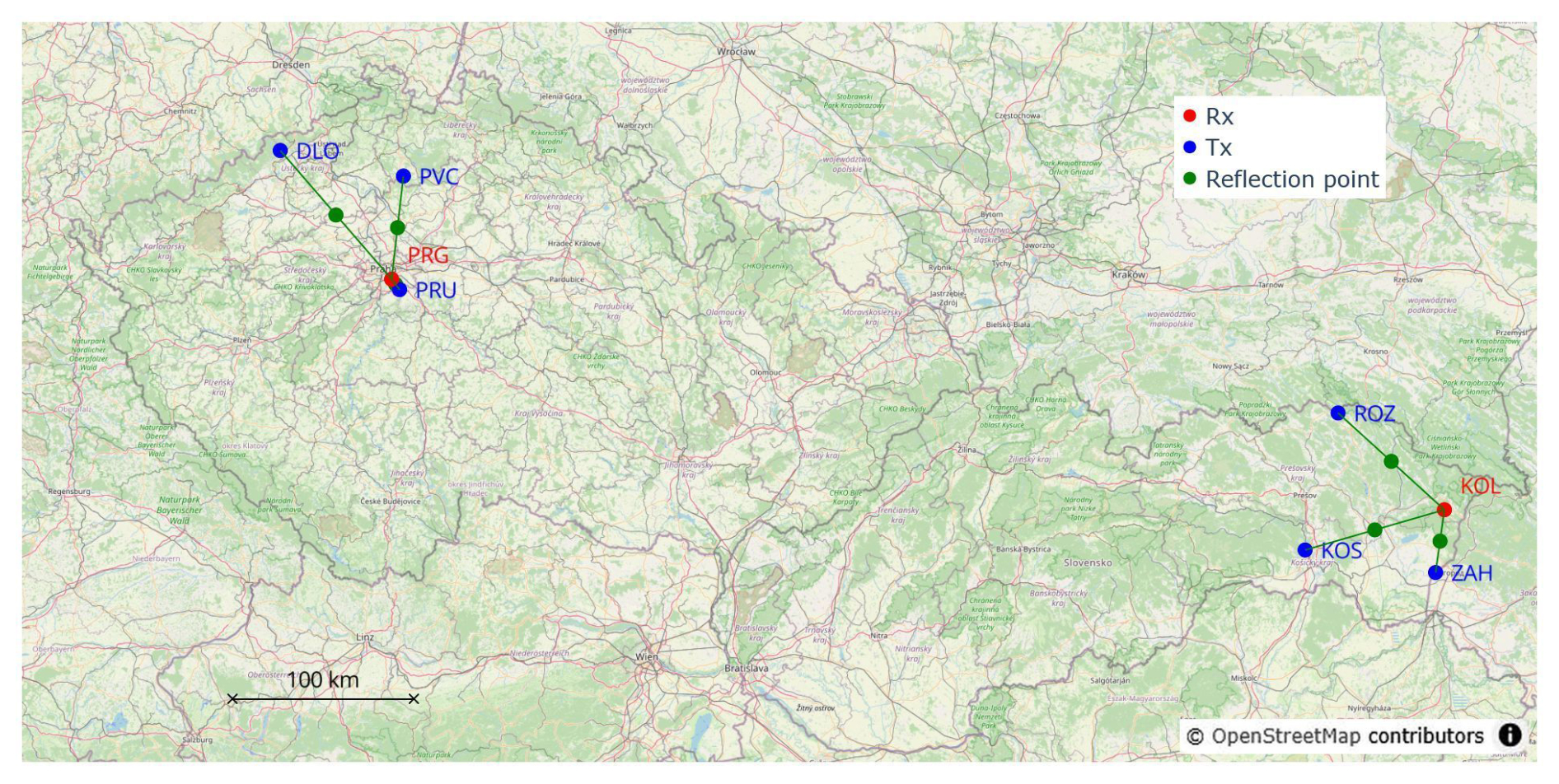
Figure 1 Distribution of CDSS transmitters (Tx, blue dots) and receivers (Rx, red dots) in Czechia and Slovakia. Digisonde DPS-4D is collocated with the Tx in Pruhonice (PRU), and the seismometer is collocated with the Tx in Panská Ves (PVC) in Czechia. © OpenStreetMap contributors (OpenStreetMap).

Reflection points of the Doppler signals, if projected to the ground, are assumed in the midpoints between each transmitter and receiver (Fig. 1). The half distances between the transmitters and receiver (few tens of km) are much smaller than the reflection heights (more than 300 km in this case). So, the sounding is quasi-vertical, which means that azimuthal angles α of sounding radio waves are small, cos(α)≈ 1, and the sounding radio waves (ordinary mode) reflect at heights where their frequency matches the local plasma frequency. If the ionospheric plasma in the reflection region moves (radially relative to the CDSS) or if the electron density changes, then the reflected radio wave experiences a Doppler shift. Assuming a sharp electron density gradient, the radial/vertical plasma velocity w_p can be computed from the obtained Doppler shift f_D as

$$\begin{array}{}\text{(1)}& w_{\mathrm{p}}=-f_{\mathrm{D}}\cdot {\displaystyle \frac{c}{\mathrm{2}{f}_{\mathrm{0}}}},\end{array}$$

where c is the speed of light and f₀ is the frequency of the sounding radio wave (Davies et al., 1962; Jacobs and Watanabe, 1966).

In the ionospheric F region, plasma is fully magnetized and moves freely only along magnetic field lines. Therefore, the vertical component of plasma motion w_p induced by vertically moving air particles with velocity w due to the infrasound waves is given by

$$\begin{array}{}\text{(2)}& w_{\mathrm{p}}=w\cdot {\sin }^{\mathrm{2}}\left(I\right),\end{array}$$

where I is the inclination of the magnetic field (∼ 66° in Czechia).

Because the plasma frequency and refractive index of the radio waves depend on the electron density, the Doppler shift is related to the electron density changes, especially at the region of reflection. Several authors (e.g., Sutcliffe and Poole, 1989 and references therein) used the equation of continuity and argued that alternating plasma compression caused by compressional magnetohydrodynamic waves should also contribute to the Doppler shift. However, the experimental results were inconclusive in the case of magnetohydrodynamic waves. Chum et al. (2012, 2016a) applied their approach and using the equation of continuity derived equation (3) which relates the observed Doppler shift f_D with the air particle vertical velocity w induced by vertically propagating infrasound waves.

$$\begin{array}{}\text{(3)}& w=-f_{\mathrm{D}}\cdot {\displaystyle \frac{c}{\mathrm{2}{f}_{\mathrm{0}}{\sin }^{\mathrm{2}}\left(I\right)}}\cdot {\displaystyle \frac{\frac{\partial N}{\partial z}}{\sqrt{(\frac{\partial N}{\partial z}{)}^{\mathrm{2}}+(N\frac{\mathrm{2}\mathit{\pi }{f}_{\mathrm{IS}}}{c_{\mathrm{s}}}{)}^{\mathrm{2}}}}},\end{array}$$

where f_IS is the infrasound frequency, c_s is the sound speed at the reflection height, N is the electron density and $\partial N/\partial z$ is the vertical gradient of the electron density at the reflection height estimated from the true height profile of the plasma frequency f_p obtained from the ionogram, e.g., by SAO Explorer software (Reinisch et al., 2005). A definition of plasma frequency f_p is used to relate f_p and N. The term $N\cdot \left(\mathrm{2}\mathit{\pi }{f}_{\mathrm{IS}}\right)/c_{\mathrm{s}}$ in the denominator of Eq. (3) results from the air/plasma compression due to the infrasound waves. See Chum et al. (2016a) for more details and derivation. Note that if ($\partial N/\partial z{)}^{\mathrm{2}}\gg (N\cdot (\mathrm{2}\mathit{\pi }{f}_{\mathrm{IS}})/c_{\mathrm{s}}{)}^{\mathrm{2}}$, then Eq. (3) reduces to Eq. (1) with usage of Eq. (2). Chum et al. (2012, 2016a) also showed that not considering the compressional term $N\cdot \left(\mathrm{2}\mathit{\pi }{f}_{\mathrm{IS}}\right)/c_{\mathrm{s}}$ can lead to results that are inconsistent with energy conservation for specific cases of the co-seismic infrasound observations.

The near surface air particle vertical oscillation velocities w₀ are determined by the vertical velocity of Earth surface motion, v_z, (Watada et al., 2006), which is measured by a seismometer co-located with PVC transmitter in the Panská Ves observatory (50.53° N, 14.57° E). The infrasound waves generated by seismic waves propagating far away from the epicentre propagate nearly vertically owing to the supersonic speed of seismic waves. Specifically, the expected zenith angle δ of the generated infrasound waves above the surface is given by Eq. (4)

$$\begin{array}{}\text{(4)}& \sin \left(\mathit{\delta }\right)={\displaystyle \frac{c_{\mathrm{s}\mathrm{0}}}{c_G}},\end{array}$$

where c_s0 is the sound speed above the ground and c_G is the speed of seismic waves (Rolland et al., 2011; Chum et al., 2016a). As c_G is about 10 times larger than c_s0, the deviation of initial infrasound wave vector from the zenith direction is around 6°.

The observed time delays between the ground surface velocities and co-seismic infrasound waves recorded by the CDSS are also compared with ray tracing simulation, including attenuation along the ray tracing trajectories due to the viscosity and thermal conductivity. The air temperature and neutral species densities at specific locations and time needed for sound speed calculation and attenuation estimate are obtained from the NRLMSIS model (Emmert et al., 2020) with a possibility to include also neutral winds using the horizontal wind model HWM14 (Drob et al., 2015). A more detailed description of the ray tracing software features can be found in Chum et al. (2023) and references therein. In addition, one-dimensional full-wave simulation of vertical infrasound propagation based on the numerical solution of the equation of continuity, the equation of motion/momentum (Navier-Stokes equation) and the heat equation using an implicit finite difference method, including non-linear terms, is performed to investigate the expected evolution of the wave spectrum with height and to estimate the expected air particle velocities at specific heights (see Chum et al., 2016b, 2018a for a more detailed description of the simulation method).

We also check other available measurements that could provide information on atmospheric waves at specific altitudes, such as airglow measurements of the hydroxyl (OH) layer in the mesopause region around 86 km using the OH temperature measurements by the Ground-based Infrared P-branch Spectrometer (GRIPS) and wave detection by the Fast Airglow Imager (FAIM) installed in Panská Ves (Schmidt et al., 2013; Hannawald et al., 2016). Both airglow instruments were setup to observe the OH layer directly below the reflection point of the CDSS (the green point between PVC and PRG in Fig. 1).

The indices of geomagnetic activity, searched to verify the geomagnetic activity, are taken from the World Data Center for Geomagnetism, Kyoto.

3 Results

Despite the maximum of solar cycle 25, the M_8.8 Kamchatka earthquake occurred during a period when ionosphere was not significantly disturbed by space weather drivers. There were no M- or X-class flares and neither strong geoeffective coronal mass ejections nor high-speed streams of solar wind plasma. Therefore, the geomagnetic activity was very low, with the following values of geomagnetic indices: Dst ∼ 12 nT and Kp ∼ 2. The conditions were therefore favourable to study the ionospheric response to acoustic-gravity waves of known origin and amplitude propagating from below. As the space weather influence was minimal (Mackovjak et al., 2026), the interpretation of the origin of the detected ionospheric variations is relatively straightforward.

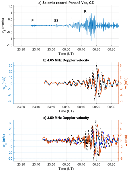
Figure 2a shows the vertical velocity v_z of ground surface motion measured in Panská Ves, Czechia, in the time interval of 70 min from the onset of the earthquake on 29 July 2025, at 23:24:52 UT. A detection of the Primary body (P) waves in Panská Ves started after 23:36 UT and continued until about 23:40 UT, with relatively small amplitudes in v_z (less than 0.1 mm s⁻¹). Secondary shear body waves once reflected from the Earth's surface (SS) were detected in the vertical component after 23:50 UT and had similar amplitudes as the P waves. The surface waves reached much larger amplitudes and were observed on 30 July 2025, approximately between 00:00 and 00:20 UT. Specifically, Long period surface (L) waves with amplitudes reaching up to around 0.4 mm s⁻¹ were observed approximately between 00:00 and 00:10 UT, and Rayleigh (R) waves with shorter periods and amplitude exceeding 1 mm s⁻¹ were recorded between 00:10 and 00:20 UT.

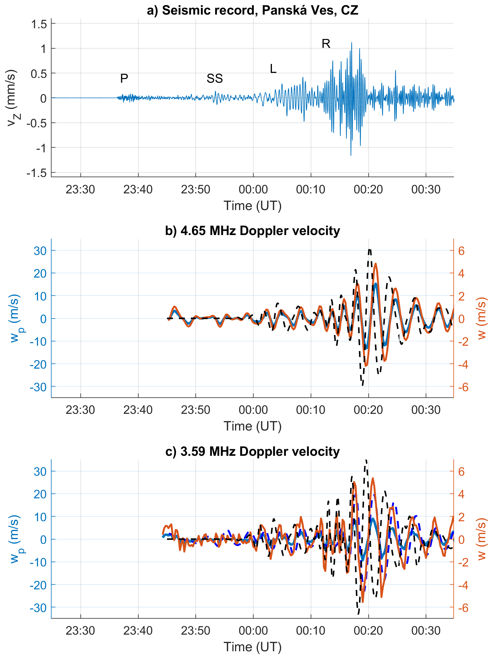
Figure 2 (a) Vertical velocity v_z of the ground surface motion in Panská Ves on the night of 29 to 30 July 2025 (b) and (c) Vertical velocity of plasma motion w_p (blue solid) directly obtained from the observed Doppler shift by Eq. (1) and the calculated vertical velocity of air particle oscillation w (red) obtained using Eq. (3) for measurements at f= 4.65 and 3.59 MHz, respectively. Black dashed lines show the simulated vertical air particle oscillation velocity at altitudes 340 and 305 km, respectively, scaled to the right axis. The blue dashed line in the plot (c) displays the w_p velocity obtained in Slovakia.

Following the activity of seismic waves, fluctuations in Doppler shifts f_D with a frequency about 0.005 Hz (period about 200 s) were observed in the CDSS records around 00:20 UT at sounding frequencies 4.65 and 3.59 MHz in Czechia (sounding frequency 7.04 MHz was above the maximum plasma frequency in the ionosphere, the critical frequency, so the 7.04 MHz signals did not reflect from the ionosphere). There were no time delays (within the time resolution) between the infrasound signals on individual sounding paths (Tx-Rx pairs), so the signals from all three transmitters were averaged at each time point. The values of the observed Doppler shifts were converted to the vertical plasma velocities w_p and vertical air particle velocities w using Eqs. (1) and (3), respectively, and after filtering out longer period fluctuations of different origin (larger than about 5 min) displayed in Fig. 2b (4.65 MHz) and Fig. 2c (3.59 MHz). The w_p and w velocities obtained from the Czech CDSS are by blue and red solid, respectively. Note different scales on the axes for the w_p (left axis) and w (right axis) velocities. The w_p velocity measured by the CDSS in Slovakia is shown by blue dashed line in Fig. 2c (the w is not calculated because of the absence of a nearby ionosonde that could provide the $\partial N/\partial z$ gradient). The signal (dominant wave packet) observed by the Czech CDSS at 3.59 MHz precedes by about 40 s the signal recorded at 4.65 MHz. The w_p amplitudes (Eq. 1) reached about 9 and 15 m s⁻¹ at 3.59 and 4.65 MHz, respectively, and the w amplitudes (Eq. 3) were about 5.5 and 4.8 m s⁻¹ at 3.59 and 4.65 MHz. The w_p amplitudes were larger at 4.65 MHz than at 3.59 MHz, whereas the w amplitudes were higher for 3.59 MHz. The reason for this is a difference in the values of electron density gradient, $\partial N/\partial z$, at reflection heights for 3.59 and 4.65 MHz waves, as will be shown later.

It is reminded that application of Eq. (3) also requires a knowledge of a dominant frequency at the reflection height to calculate w. An insight in a spectral content of the observed waves and their evolution with time is shown in dynamic spectra displayed in Fig. 3. It is important to note that the seismic wave packet labelled L (Figs. 2a and 3a) contains a very broad frequency spectrum, including frequencies around 0.005 Hz, which are detected also in the Doppler shift records (Fig. 3b and c), approximately 11–13 min later. The frequency of 0.005 Hz was used to calculate w shown in Fig. 2b and c.

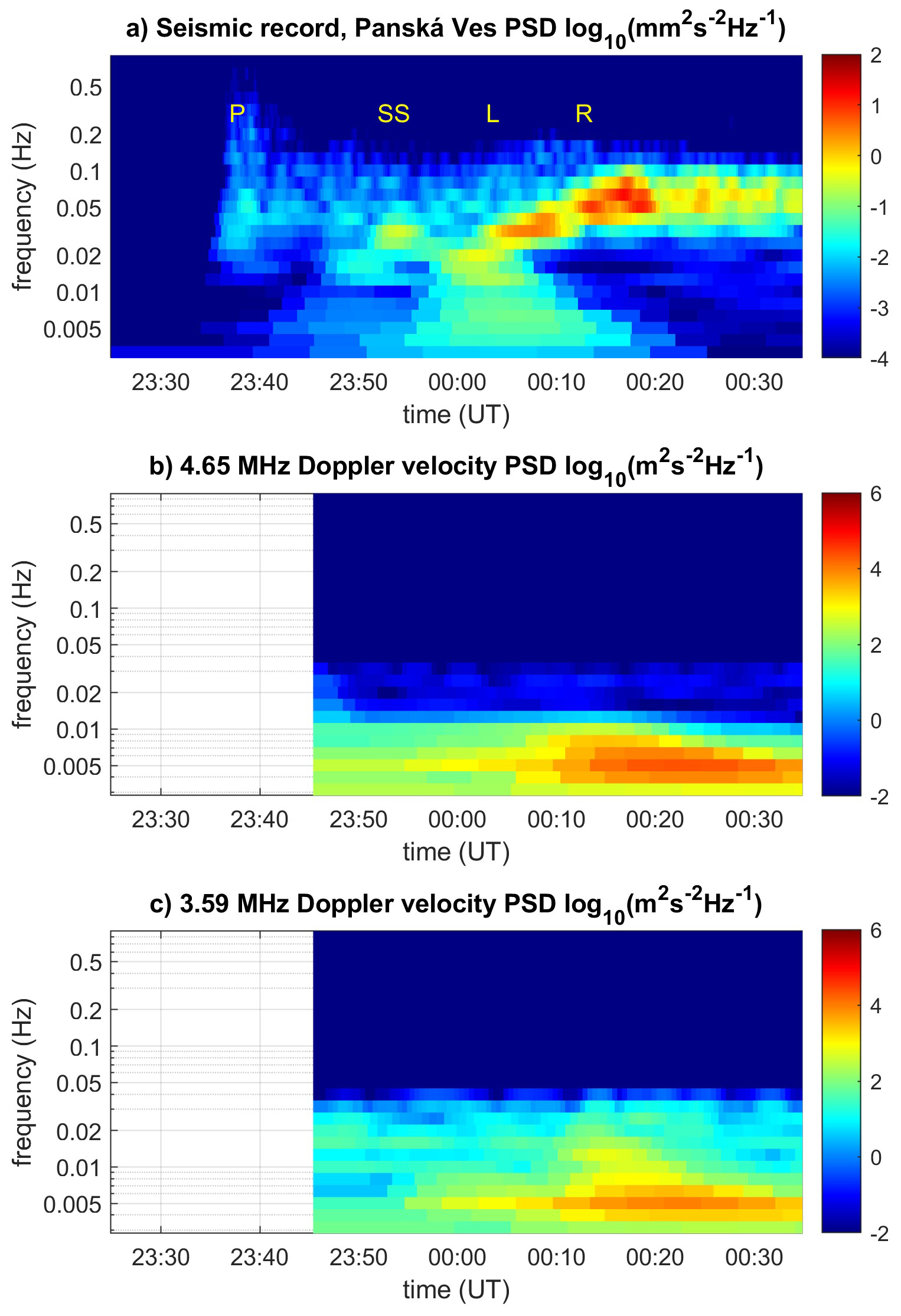
Figure 3 Dynamic spectra (power spectral densities) of vertical velocity v_z of the ground surface motion on the night of 29 to 30 July 2025 (a), and of the Doppler shifts measured at f= 4.65 MHz (b) and 3.59 MHz (c). The dynamic spectra correspond to signals presented in Fig. 2.

The reflection heights of the ordinary mode of the sounding radio waves with frequencies 3.59 and 4.65 MHz are about 305 and 340 km, respectively, as shows the height profile of plasma frequency (true height profile) obtained from the ionogram recorded in Pruhonice on 30 July at 00:25 UT, which is displayed in Fig. 4. The average reflection heights for the 3.59 and 4.65 MHz waves in the time interval from 00:10 to 00:30 UT obtained from a sequence of ionograms are 303 and 336 km, respectively. Figure 4 also shows the estimated inverse of the plasma density gradients at the reflection heights, from which the electron density gradient $\partial N/\partial z$ is obtained using the definition of plasma frequency f_p. The obtained values are ∂N/$\partial z=$ 3.56 × 10⁶ and 2.75 × 10⁶ m⁻⁴ at the reflection heights of 3.59 and 4.65 MHz waves, respectively. These values were used to calculate vertical air particle velocities w plotted in Fig. 2b and c.

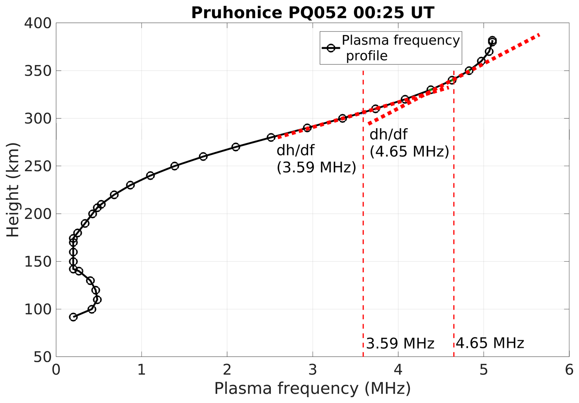
Figure 4 True height profile of plasma frequency derived from the measurements by the digisonde located in Průhonice, PQ052, on 30 July 2025 at 00:25 UT. The CDSS sounding frequencies 3.59 and 4.65 MHz and the vertical plasma density gradients are marked by red.

To verify that the observed time delays correspond to the propagation of infrasound waves, which are a probable cause of the ionospheric disturbances, we performed a ray tracing simulation. Figure 5a shows the simulated propagation time (orange) and sound speed (black) of the infrasound waves launched with the zenith angle 6° from the Panská Ves location on 30 July 2025 at 00:06 UT. The propagation times to altitudes 305 and 340 km are 680 and 724 s, respectively. The sound speeds at these altitudes are 807 and 837 m s⁻¹, respectively. The modelled propagation times are consistent with the observed time delays between the 0.005 Hz signal recorded on the ground by the seismometer and in the ionosphere by the CDSS at about 305 and 340 km altitudes.

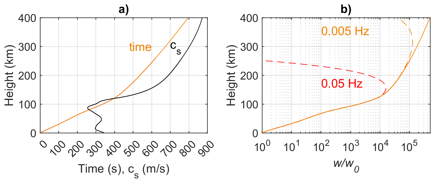
Figure 5 (a) Simulated infrasound propagation time (orange) and sound speed (black) as a function of height. (b) Simulated vertical air particle oscillation velocities w normalized to the initial value w₀ above the ground surface for frequencies 0.05 Hz (red) and 0.005 Hz (orange). The solid orange line represents an idealized case of lossless propagation of a plane wave.

Dashed lines in Fig. 5b show the ratios $w/w_{\mathrm{0}}$, which represent the expected/simulated vertical air particle velocities w at a specific altitude normalized by their near surface value w₀, including the frequency dependent attenuation along the ray trajectories for infrasound frequencies 0.05 (red) and 0.005 (orange) Hz. The solid line displays the expected ratio for an unrealistic lossless (infra)sound plane wave propagation for which the infrasound power flux is conserved. It means that the quantity c_sρw² is constant, where ρ is the air density, decreasing exponentially with height (obtained from the NRLMSIS model). Figure 5b shows that waves with a frequency of 0.05 Hz begin to be significantly attenuated above an altitude of approximately 150 km. On the other hand, the 0.005 Hz waves can reach the height of 300 km without a significant attenuation. The ratio $w/w_{\mathrm{0}}$ (normalized velocity w) for 0.005 Hz waves at the observation heights 305 and 340 km is 1.26 × 10⁵ and 1.19 × 10⁵, respectively. For idealized lossless propagation it is 1.89 × 10⁵ and 2.74 × 10⁵, respectively, at these heights.

It is important to stress that a comparison of the observed values w(w_p) displayed in Fig. 2 with the simulated values w shown in Fig. 5b is not straightforward. The reason is that the calculated normalized values $w/w_{\mathrm{0}}$ correspond to monochromatic waves. The wave attenuation with height strongly depends on the wave frequency. The higher frequency, the lower is the altitude at which the wave energy dissipates (Fig. 5b). Figure 3a shows that the seismic wave packet L contained a very wide range of frequencies and therefore generated infrasound in a broad frequency spectrum. However, only the waves corresponding to frequencies around 0.005 Hz – a small energy fraction could reach the heights above 300 km, where the induced plasma fluctuations were detected by the CDSS. Therefore, for the wave packet L it makes no sense to compare the observed amplitudes w(w_p) normalized by the v_z amplitude (Fig. 2) with the simulated ratio $w/w_{\mathrm{0}}$ (Fig. 5b).

To compare the observed amplitudes obtained from the CDSS measurements with the expected values, we performed full wave one-dimensional numerical simulation of infrasound propagation in the vertical direction, started with initial perturbations above the Earth's surface defined by the vertical motion of the ground surface, w₀=v_z. The assumption of this initial perturbation is based on theoretical work (Watada et al., 2006) and was successfully applied in previous studies (Chum et al., 2018a and references therein). The w values obtained by the full-wave numerical simulation at the heights 305 and 340 km are plotted in Fig. 2c and b, respectively, by the dashed black lines. The values are scaled to the right (w) axis and the maximum amplitudes are about 6.8 m s⁻¹ at 305 km and 6.2 at 340 km. It means that they are about 30 % larger than the w values estimated from the measurement. The main fluctuations of the simulated waveforms occur at approximately similar times as the w(w_p) values derived from the observed Doppler shifts and have also similar frequencies. The simulated signals only slightly advance the observation. Therefore, the simulation agrees reasonably well with the observation. It should be noted in this respect, that the real trajectory of infrasound waves will be somewhat longer than the vertical distance due to the non-zero zenith angle of propagation and due to the neutral winds, which may affect the trajectory. Consequently, the location of the seismometer in Panská Ves (PVC in Fig. 1) used for the simulation may not be the exact source location of the waves that reach the observation points.

Figure 6 shows the height evolution of the air particle velocity fluctuation spectra obtained by the one-dimensional full-wave numerical simulation started with the fluctuations defined by the seismic record, w₀=v_z. The power spectral densities of w are normalized to their maximum value above the ground surface and their colour-coded common logarithm is displayed in Fig. 6. The height-dependent spectra in Fig. 6 confirm that only waves with the lowest frequencies (about 0.005 Hz) can reach the observation altitudes, although they carry just a small fraction of the total wave energy at altitudes lower than about 200 km.

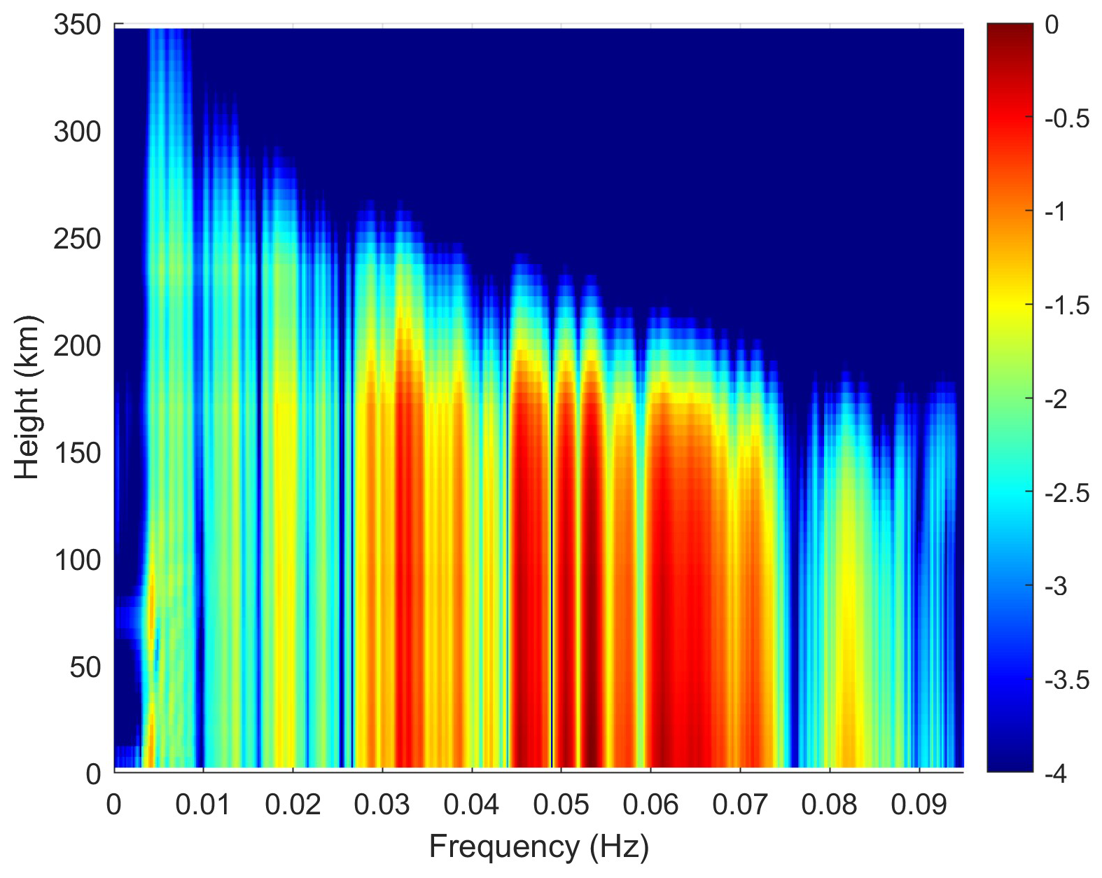
Figure 6 Expected power spectral densities (colour coded common logarithm) at different altitudes, normalized to the ground level.

We also investigated measurements that could provide information about wave propagation at lower heights, namely OH airglow emissions originating from an about 10 km thick layer around 86 km, which may be modulated by co-seismic atmospheric waves (Snively, 2013; Wüst et al., 2023). Figure 7 shows that no significant changes in the OH temperature related to the infrasound waves were detected over Czechia, despite intensity drops in the used OH(3-1)- and OH(4-2)-Q-branches, approximately in the interval from 00:05 to 00:35 UT, which roughly coincides with the occurrence of the co-seismic infrasound waves. On the one hand the ratio of these two emissions serves as a cloud indicator (OH(3-1)-Q at 1.505 µm is more strongly attenuated by water and ice droplets compared to OH(4-2)-Q at 1.585 µm). On the other hand, both emissions originate at slightly different centroid altitudes, separated by 0.5–1.0 km (e.g., von Savigny et al., 2012). Atmospheric waves with short vertical wavelengths (≪ 100 km) passing through the OH layer will therefore leave a clear signature in the OH(3-1)/OH(4-2)-ratio, while waves with large vertical wavelengths (affecting both emissions at the same time) will not (Schmidt et al., 2018). This drop in intensity without a significant change in the OH(3-1)/OH(4-2)-ratio indicates the presence of an atmospheric structure with large vertical scales, which is in contrast with the expected wavelength of the co-seismic infrasound (about 6 km for the dominant 0.05 Hz waves at this altitude and about 60 km for the 0.005 Hz waves). Model results by Inchin et al. (2020, 2022) predicted a drop in intensity by about 15 %, but only close to the epicenter. Data from the OH imager (FAIM) show the presence of a varying number of small clouds in the fields of view of both instruments at this time. A similar drop in OH intensities were not observed in other European stations equipped with the OH imagers and spectrometers in this time interval. Thus, the co-seismic origin of the observed intensity drop remains questionable. The time resolution of OH temperature measurement by GRIPS is 15 s. This sampling frequency does not allow for the analysis/detection of waves with a dominant frequency of approximately 0.05 Hz, which is expected at the height of the OH layer (Fig. 6). The waves with frequency around 0.005 Hz were not detected in the OH temperature time series at the expected time (around 00:10 UT on 29 July 2025) using the continuous Wavelet Transform (not shown). The reason may be an insufficient signal-to-noise ratio (SNR), as the model predictions by Inchin et al. (2020, 2022) show that co-seismic airglow perturbations range between 1 %–5 % and are weaker in temperature than in intensity requiring an SNR that wasn't reached during this particular night (Fig. 7).

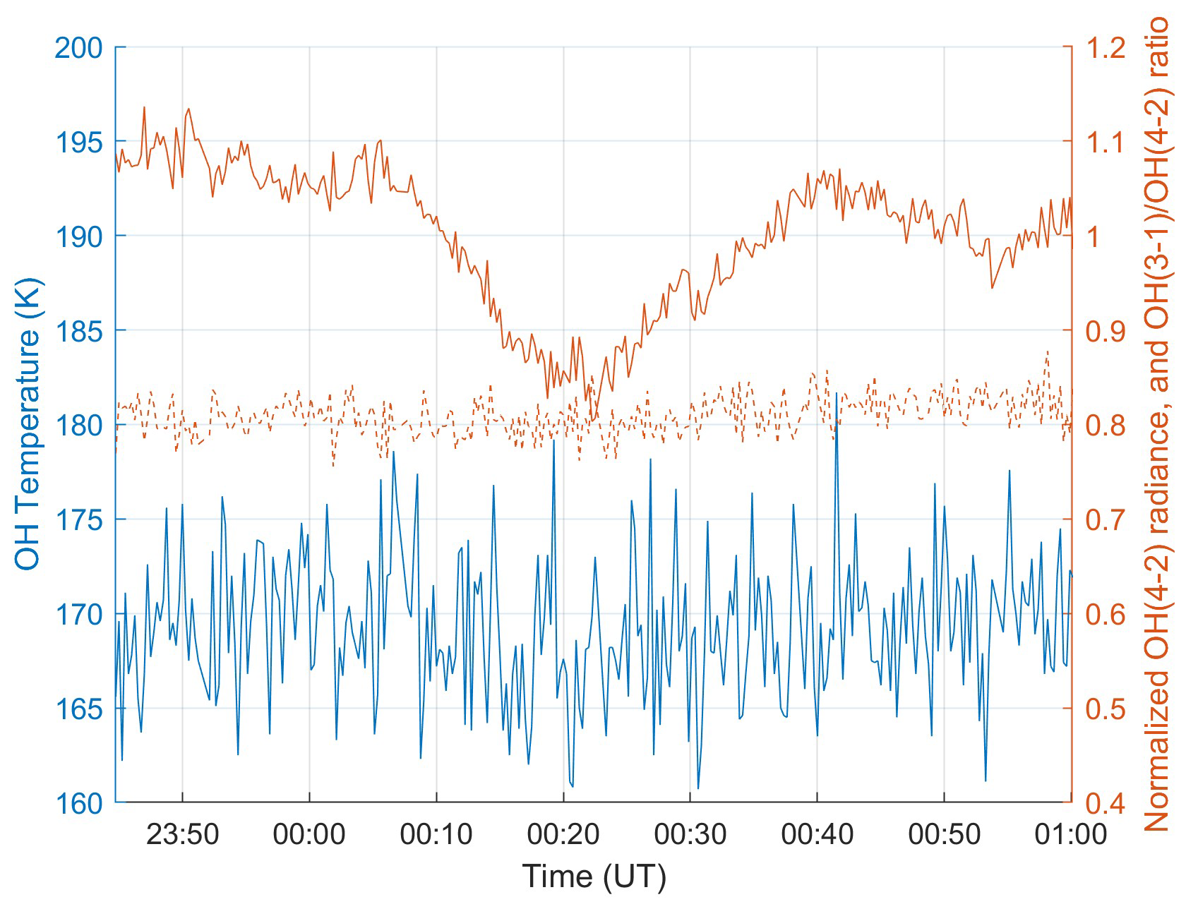
Figure 7 OH temperature (blue) and OH(4-2) radiance (solid red) on the night of July 29 to 30, 2025. The nearly constant ratio (dashed red) between OH(3-1)- and OH(4-2)-emissions indicates a structure with large vertical wavelengths/scales being associated with the drop in intensity. See text for further details.

4 Discussion and Conclusions

The simulated air particle vertical velocities w shown in Fig. 2 by black dashed lines are about 30 % larger than the values obtained from observation using Eq. (3). This is a reasonable agreement considering the uncertainties in determination of $\partial N/\partial z$ gradients (around 10 %). Importantly, it is reasonable to expect that the observed w are smaller, than the simulated values for several reasons. First, the simulation is based on the plane wave propagation (one-dimensional simulation) and does not take into account a possible divergence of infrasound ray trajectories, and therefore does not consider a decrease of the infrasound power flux due to the geometrical spreading of the waves. Second, the simulation only considers attenuation due to the viscosity and thermal conductivity (Chum et al., 2016b), but does not simulate other possible losses, for example, rotational relaxation losses, turbulent losses etc. (Bass et al., 1984). Third, the actual trajectory of infrasound waves may be longer than the pure vertical distance, and consequently the attenuation larger, due to the non-zero zenith angle and due to the neutral winds. It is useful to stress that both the plasma velocities w_p and the air particle velocities obtained directly from w_p by using Eq. (2), without including the compressional term, give values roughly 100 % larger than the simulated values, which is highly improbable for the reasons mentioned above, and indicates the need to use the compressional term in the quantitative analysis of infrasound amplitudes using Doppler shift measurements.

The observed time delay of about 12 min between the 0.005 Hz waves in the seismic record and the waves of the same frequency in the Doppler shift (air particle velocity fluctuations) is consistent with the numerical simulation of infrasound propagating in the (quasi)vertical direction. In addition, the 3.59 MHz CDSS in Czechia detects the co-seismic signal approximately 40 s sooner than the 4.65 MHz CDSS, the signal of which is reflected at the altitude about 35 km higher.

The Slovak 3.59 MHz CDSS detects the co-seismic infrasound waves at a similar time as the Czech CDSS, with a phase shift locating the main fluctuations roughly between the 3.59 and 4.65 MHz signals in Czechia (Fig. 2c). This indicates that the reflection height for the 3.59 MHz radio waves is somewhat larger in Slovakia than in Czechia, considering (quasi)vertical propagation of infrasound and similar horizontal distances from the epicentre (about 8150 km the Czech CDSS and about 8060 km the Slovak CDSS). The vertical plasma velocities w_p obtained without considering the compressional term (Eq. 1) are about 100 % higher in Slovakia than in Czechia. It is reminded that there is no nearby ionosonde in Slovakia that would provide reliable $\partial N/\partial z$ values for calculating the more realistic velocities w using Eq. (3). However, if we assume that the air particle velocities w are approximately the same over Czechia and Slovakia, then it follows from Eq. (3) that the electron density gradient $\partial N/\partial z$ at the corresponding reflection heights of 3.59 MHz signals must be smaller in Slovakia, than in Czechia. This is consistent with the higher reflection height in Slovakia deduced from the timing mentioned above (note that $\partial N/\partial z$ usually decreases with height in the F2 layer, when approaching the peak of the layer).

Unlike the previous observation of co-seismic infrasound waves by CDSS in Czechia, triggered by strong earthquakes, namely M_9.0 Tohoku 2011, M_7.8 Nepal 2015, and M_7.7 Turkey 2023 earthquakes, when the shape and spectral content of the wave packets in the co-seismic Doppler shift fluctuations was very similar to that recorded in the vertical velocity v_z of ground surface motion (Chum et al., 2012, 2016a; Haralambous et al., 2023), the spectral content of the detected co-seismic ionospheric waves associated with the M_8.8 Kamchatka earthquake differed significantly from v_z. The main reason for that is the high altitude of observation and filtering out of waves with higher frequencies during the infrasound propagation to such a high altitude, including waves with frequencies that are dominant at lower altitudes. This is a novel observation, which contributes to a better understanding of propagation of the co-seismic infrasound to high altitudes, approximately up to the peak of the ionosphere.

It should be stressed that the change of the wave packet shape and absence of waves with higher frequencies at the CDSS observation height in this case is not caused by nonlinear effects, which are a consequence of large amplitude of infrasound waves in the upper atmosphere that may occur for sufficiently strong initial perturbations w₀=v_z (Chum et al., 2016b; Chum et al., 2018a), but purely by filtering out of waves with higher frequencies due to the wave attenuation, which strongly depends on wave frequency. Unlike the case of nonlinear effects (Chum et al., 2016b), a nonlinear simulation started with an initial perturbation $w_{\mathrm{0}}=v_z/\mathrm{10}$ provides in this case practically the same wave packet (spectral content) at the observation altitude, only with ∼ 0.1 amplitude, when compared with the simulation started for w₀=v_z.

The co-seismic infrasound waves have never been observed at ∼ 340 km height by the CDSS in Czechia before. All the previous Czech observations of co-seismic infrasound were from an altitude range approximately 150–220 km. To the best of our knowledge, we are not aware of any Doppler observation of co-seismic infrasound in such a height in other countries. It is reminded that although TEC perturbations detected by GNSS receivers are usually mapped to the peak of F2 layer, they are usually observed with a 8–9 min delay with respect to the seismic record (Astafyeva, 2019; Wüst et al., 2026 and references therein), which indicates dominant perturbations at ∼ 250 km or below when considering the expected sound speed height profile (e.g., Fig. 5a). There is actually no direct information about the altitude of the TEC disturbance due to the height integrated nature of the TEC GNSS measurements. In addition, we have not identified any TEC perturbations over the Central Europe that could be reliably associated with the co-seismic infrasound. On the other hand, ionospheric disturbances associated with tsunami waves were with a high probability detected at the altitudes above 400 km by Low Earth Orbit satellites (Yang et al., 2022; Alfonsi et al., 2024), but these perturbations are related to the gravity waves, rather than to infrasound. Therefore, the detection of infrasound waves in the ionosphere by the CDSS at the height of around 340 km and about 12 min after the arrival of causative Long period surface seismic waves is a unique observation, which experimentally proves that low frequency infrasound waves can reach such a high altitude. It should also be remembered that the detailed analysis of the co-seismic infrasound observed by the CDSS was possible due to the operation of a nearby digisonde which provided the reflection heights of the CDSS signals and electron density gradients there.

Appendix A: List of abbreviations

CDSS	continuous Doppler sounding system
GNSS	global navigation satellite system
OH	hydroxyl
Rx	receiver
TEC	total electron content
Tx	transmitter
UT	universal time