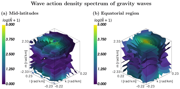
Variability of local gravity wave spectra from data of a high-resolution icosahedral-grid global model

Atmospheric gravity waves influence the general circulation through transport of energy and momentum. Even with increasing computing capacities, parametrisation of their effects is still needed. Here, we diagnose gravity wave spectra from the data of a high-resolution ICON simulation on subdomains defined by a low-resolution ICON grid. A unique methodology is applied that avoids unnecessary interpolations and filters the data by projection on the linearised gravity wave modes, providing precise and detailed information about the gravity wave spectra. The dependence of these spectra on latitude is then studied, highlighting the importance of the zonal wind direction in the shape of the spectra. Finally, we see that the spectra can be highly simplified by using tens to hundreds of principal components, which is a key property allowing for an increase in efficiency of current gravity wave parametrisations.

1 Introduction

Gravity waves (GWs) are a ubiquitous phenomenon in the atmosphere, influencing the atmospheric wind field by both dissipative and non-dissipative effects (Sutherland, 2010). They redistribute energy and momentum, which significantly affects large-scale stratospheric dynamics (Fritts and Alexander, 2003; Sacha et al., 2021), drives the quasi-biennial oscillation in the middle atmosphere (Ern et al., 2014; Corcos et al., 2025), and is also linked to interannual variability such as the El Niño–Southern Oscillation or North Atlantic Oscillation (Sato et al., 2016; Procházková et al., 2025; Kawatani et al., 2025). Moreover, GWs influence the transport of particles in the atmosphere (Chane Ming et al., 2016) and play a role in cloud physics (Plougonven et al., 2015; Dolaptchiev et al., 2023; Achatz et al., 2024).

As GWs act on various scales, with horizontal wavelengths between few and thousands of kilometres, only a part of their spectra is resolved by global numerical models, and the effects of the under- and unresolved waves have to be parametrised. Although the resolution of current simulations of the weather and climate system has been improving, GW parametrisations still need to be included (Polichtchouk et al., 2023). Currently used parametrisations for both orographic and non-orographic GW generally prescribe the GW sources, possibly in the form of GW spectra, and the way they propagate in the atmosphere and dissipate at certain levels, causing acceleration or deceleration of the mean flow through deposition of energy (Schirber et al., 2014; Plougonven et al., 2020). The parametrisations are most often highly simplified, and our knowledge of the input of parametrisations, especially for non-orographic and non-convective GW sources, is also limited (Plougonven et al., 2020; Achatz et al., 2024), with the sources often described using simplified or even universal spectral shapes, such as the Desaubies spectrum (Bölöni et al., 2021). This implies that the variability of initial GW spectra is assumed to be small or dynamically irrelevant. However, observational and modelling evidence suggests that GW generation is highly intermittent and source-dependent (e.g., Hertzog et al., 2012; Plougonven and Zhang, 2014), which raises the question of whether a universal spectral representation is sufficient for capturing their effects on the large-scale flow. In this work, we address the problem of assessing spectra variability with the aim of improving parametrisations by a spectral analysis of a high-resolution model simulation.

One-dimensional spectra describing atmospheric waves using temperature or wind velocities have already been studied for a few decades in both theory and observations (e.g., Nastrom and Gage, 1985; Lindborg, 1999; Stephan et al., 2022; Morfa and Stephan, 2023, 2025). The processes in the atmosphere are then attributed to the slope of the spectra. In particular, the mesoscale −5/3-slope is observed in the upper troposphere and lower stratosphere, with a possible explanation linked to inertia-gravity waves (Morfa and Stephan, 2025). A spectrum decomposition approach is followed by Žagaragar et al. (2015), distinguishing between balanced and unbalanced flow spectra by representing the global circulation in terms of normal-mode functions. However, this methodology does not allow the spectra to be evaluated at local domains for visualizing the wave field at specific locations. Moreover, up-to-date studies usually focus on the averaged 1D spectra, not considering a potential directionality or anisotropy of the observed processes (e.g., Becker et al., 2022; Liu et al., 2024; Okui et al., 2022).

Here, we investigate whether GW spectra exhibit significant spatial variability and whether this variability can be represented in a reduced form suitable for parametrizations. To this end, we calculate local three-dimensional GW spectra at subdomains defined by a low-resolution model grid. We introduce a novel methodology that uses data restricted to the triangular subdomains and projects the spectra to GW modes using linear GW theory. The variability of the spectra among the coarse-grained triangular grid cells is analysed by applying the principal component analysis.

The goal is to assess whether GW spectra can be approximated by a small number of dominant patterns, or whether their variability is too large to justify the use of fixed spectral shapes. This provides a direct link to the development of parametrisations: if the spectra are low-dimensional but variable, they may be predicted from large-scale conditions, for example using machine learning approaches. While the implementation of such parametrizations is beyond the scope of this study, the results presented here establish the necessary foundation by quantifying the structure and variability of resolved GW spectra.

In Sect. 2, we describe the methods and data used for the analysis, with the emphasis on the newly introduced approaches. The methodology is then illustrated in Sect. 3.1 and 3.2, followed by the analysis of the variability of GW spectra in Sect. 3.3. The results are discussed and conclusions presented in Sect. 4.

2 Data and methodology

In order to assess the variability of the gravity waves, local 3D spatio-temporal spectra are computed and projected onto the gravity wave part defined by the linear theory, as described by the following subsections. Resulting gravity wave spectra are analysed using principal component analysis. The individual steps are described below.

2.1 ICON simulation

The analysis is performed on a global simulation of the Icosahedral Nonhydrostatic model (ICON) on a model grid R2B10 with an approximate horizontal resolution of 2.5 km. The data cover the period from 23 to 29 January 2020 with an output time step of 10 min. Due to the high resolution, no parametrisation of GWs is applied. We used the model output interpolated to the vertical level of 15 km.

For assessing the local effects, the data are divided into subdomains defined as the cells of the ICON R2B4 grid (160 km resolution). In this way, we are estimating the effect that would be missing if only a low-resolution model was applied instead of using the R2B10 grid, in the range of wavelengths admissible by the analysis and excluding the interaction of scales. Although we are missing some GWs even in the high-resolution simulation (Polichtchouk et al., 2023), these waves, as well as waves removed during the analysis due to the effective resolution limit, have short wavelengths and therefore we do not expect a significant influence on the results in the wavenumber ranges studied.

2.2 Local spectra

The computation of the three-dimensional spectra at the subdomains is done in two steps, by transforming the data first in wavenumber and then in frequency domain. For each subdomain, the data are first used to compute the time series of horizontal spectra. Afterwards, 1D Fourier transform is applied to the resulting time series of horizontal spectral coefficients, adding the frequency dimension to the spectra.

The computation of the horizontal spectrum is more involved because the data are defined on a triangular ICON grid and the subdomains are triangular as well. With some modification, we apply the procedure of Least-squares Fourier fitting (Lomb, 1976; Scargle, 1982), used for a similar procedure for physical orography in Chew et al. (2024).

For each subdomain, the computation is done in the local Cartesian system with the origin in the circumcentre of the triangle, the x axis pointing to the east, and the y axis pointing to the north. The projection of the points from the high-resolution grid to this local system is constructed by projecting the points from the sphere to the plane defined by the vertices of the triangle.

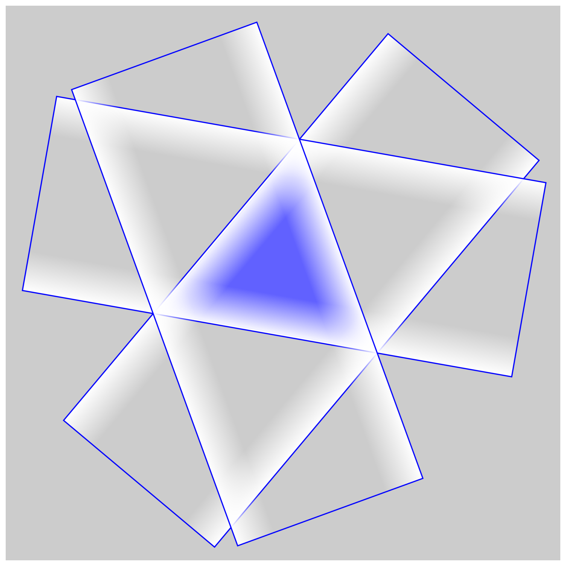
In the first step, the field on the triangle is deplaned and tapered. For tapering, the 1D Tukey window with parameter α=0.2 and width being the height of the triangle is applied in the three directions perpendicular to the sides of the triangular subdomain, as illustrated in Fig. 1. This creates zero values on the sides and at the opposite apices. In the corners, the tapering is more effective, with the 1D Tukey window also applied with each adjacent side, which is very similar to standard 2D tapering methods in rectangular domains (Blažica et al., 2015). The deplaning is done by subtracting plane fitted to the data in the triangle, using the linear approximation approach introduced in Powell (1994).

Figure 1 Illustration of the taper applied on the triangular subdomains.

In the next step, the zonal and meridional wavenumbers of the spectra are defined. For this, the average horizontal resolution of the high-resolution data dx, as given by ICON, and the horizontal extent of the subdomains L_x and L_y, defined as the zonal and meridional sides of the smallest rectangle in which the subdomain can be inscribed, are used:

$$\begin{array}{}\text{(1)}& {\displaystyle }{k}_i& {\displaystyle }={\displaystyle \frac{\mathrm{2}\mathit{\pi }{m}_i}{N_x\mathrm{d}x}},m_i=\mathrm{0},\mathrm{\dots },\lfloor {\displaystyle \frac{L_x}{\mathrm{2}\mathrm{d}x{M}_n}}\rfloor -\mathrm{1},\text{(2)}& {\displaystyle }{l}_j& {\displaystyle }={\displaystyle \frac{\mathrm{2}\mathit{\pi }{m}_j}{N_y\mathrm{d}x}},m_j=-\lfloor {\displaystyle \frac{L_y}{\mathrm{d}x{M}_n}}\rfloor /\mathrm{2}+\mathrm{1},\mathrm{\dots },\lfloor {\displaystyle \frac{L_y}{\mathrm{d}x{M}_n}}\rfloor /\mathrm{2},\end{array}$$

where $N_x=L_x/\mathrm{d}x$, $N_y=L_y/\mathrm{d}x$ and M_n is a parameter that allows the computation of only a part of the spectrum. Here, the symbol ⌊⋅⌋ represents the closest even number. To avoid computation of a large part of the spectrum below effective resolution, M_n=4 is used and we define the notation ${\stackrel{\mathrm{̃}}{N}}_x/\mathrm{2}=\lfloor L_x/\mathrm{2}\mathrm{d}x{M}_n\rfloor$ and ${\stackrel{\mathrm{̃}}{N}}_y=\lfloor L_y/\mathrm{d}y{M}_n\rfloor$. Since the data are real, we compute the horizontal spectrum only for positive zonal wavenumbers. After finding the horizontal spectrum with these wavenumbers, the part of the spectrum for the negative zonal wavenumber is completed by using the symmetry of the Fourier transform. In our data, ${\stackrel{\mathrm{̃}}{N}}_x$ and ${\stackrel{\mathrm{̃}}{N}}_y$ reach values around 20, based on the subdomain size.

With the wavenumbers defined by Eqs. (1) and (2), the amplitudes of the Fourier transform are fitted, so that

$$\begin{array}{}\text{(3)}& \begin{array}{rl}& f(x,y)\\ & \approx \sum _{j=\mathrm{0}}^{{\stackrel{\mathrm{̃}}{N}}_y/\mathrm{2}}\left[\mathrm{2}{\widehat{f}}_{\mathrm{0},j}^{\left(r\right)}\cos \left(l_{j}y\right)-\mathrm{2}{\widehat{f}}_{\mathrm{0},j}^{\left(i\right)}\sin \left(l_{j}y\right)\right]+\sum _{i=\mathrm{1}}^{{\stackrel{\mathrm{̃}}{N}}_x/\mathrm{2}-\mathrm{1}}\\ & \sum _{j=-{\stackrel{\mathrm{̃}}{N}}_y/\mathrm{2}+\mathrm{1}}^{{\stackrel{\mathrm{̃}}{N}}_y/\mathrm{2}}\left[\mathrm{2}{\widehat{f}}_{i,j}^{\left(r\right)}\cos (k_{i}x+l_{j}y)-\mathrm{2}{\widehat{f}}_{i,j}^{\left(i\right)}\sin (k_{i}x+l_{j}y)\right]\\ & \equiv F\left[\widehat{f}\right],\end{array}\end{array}$$

where ${\widehat{f}}_{i,j}^{\left(r\right)}$ and ${\widehat{f}}_{i,j}^{\left(i\right)}$ are the real and imaginary components of the Fourier amplitudes $\widehat{f}={\widehat{f}}_{i,j}^{\left(r\right)}+i{\widehat{f}}_{i,j}^{\left(i\right)}$ and F is an operator mapping $\widehat{f}$ to the approximation of the inverse Fourier transform, as defined by Eq. (3). The fitting is achieved by minimisation of the functional

$$\begin{array}{}\text{(4)}& J\left[\widehat{f}\right]=\Vert f-F\left[\widehat{f}\right]{\Vert }^{\mathrm{2}}+\mathit{\lambda }\Vert \widehat{f}{\Vert }^{\mathrm{2}}.\end{array}$$

The regularizing term $\mathit{\lambda }\Vert \widehat{f}\Vert$ is necessary to avoid overfitting. The minimiser can be obtained by evaluating the Gateaux derivative of the functional J and setting it to zero, which leads to the equation

$$\begin{array}{}\text{(5)}& (F^{T}F+\mathit{\lambda }I)\widehat{f}=F^{T}f,\end{array}$$

with $\widehat{f}$ being represented by a 1D vector composed of the individual values of ${\widehat{f}}_{i,j}^{\left(r\right)}$ and ${\widehat{f}}_{i,j}^{\left(i\right)}$ and F by a matrix containing terms 2cos (k_ix+l_jy) and $-\mathrm{2}\sin (k_{i}x+l_{j}y)$ from Eq. (3).

The regularization parameter λ is chosen as 0.1 times the average of the diagonal coefficients of the matrix F^TF. Equation (3) describes the real Fourier transform and its equivalence to the formula for standard Fourier transform with both negative and positive wavenumbers up to the choice of truncation limits, is shown in Chew et al. (2024).

The temporal spectrum is computed from the horizontal spectrum coefficients by 1D FFT

$$\begin{array}{}\text{(6)}& \widehat{\widehat{f}}(k,l,{\mathit{\omega }}_n)=\sum _{r=\mathrm{0}}^{N_t-\mathrm{1}}\widehat{f}(k,l,t_r)e^{-\mathrm{i}{\mathit{\omega }}_n{t}_r},\end{array}$$

where N_t is the number of time steps t_k considered for the transform and ${\mathit{\omega }}_n=-\mathrm{2}\mathit{\pi }n/T$ with T being the length of the time series. For the daily spectra of the data with a time step of 10 min, we have N_t=144. Note the negative sign in the definition of ω that allows us to write

$$\begin{array}{}\text{(7)}& \begin{array}{rl}f(x,y,t)& ={\displaystyle \frac{\mathrm{1}}{N_t}}\sum _{i=-{\stackrel{\mathrm{̃}}{N}}_x/\mathrm{2}+\mathrm{1}}^{{\stackrel{\mathrm{̃}}{N}}_x/\mathrm{2}-\mathrm{1}}\sum _{j=-{\stackrel{\mathrm{̃}}{N}}_y/\mathrm{2}+\mathrm{1}}^{{\stackrel{\mathrm{̃}}{N}}_y/\mathrm{2}-\mathrm{1}}\\ & \sum _{r=\mathrm{0}}^{N_t-\mathrm{1}}\widehat{\widehat{f}}(k_i,l_j,{\mathit{\omega }}_r)e^{\mathrm{i}(k_{i}x+l_{j}y-{\mathit{\omega }}_{r}t)}\end{array}\end{array}$$

with the inverse transform

$$\begin{array}{}\text{(8)}& \begin{array}{rl}\widehat{\widehat{f}}(k,l,\mathit{\omega })& ={\displaystyle \frac{\mathrm{1}}{{\stackrel{\mathrm{̃}}{N}}_k{\stackrel{\mathrm{̃}}{N}}_l}}\sum _{i=-{\stackrel{\mathrm{̃}}{N}}_x/\mathrm{2}+\mathrm{1}}^{{\stackrel{\mathrm{̃}}{N}}_x/\mathrm{2}-\mathrm{1}}\sum _{j=-{\stackrel{\mathrm{̃}}{N}}_y/\mathrm{2}+\mathrm{1}}^{{\stackrel{\mathrm{̃}}{N}}_y/\mathrm{2}-\mathrm{1}}\\ & \sum _{r=\mathrm{0}}^{N_t-\mathrm{1}}f(x_i,y_j,t_r)e^{-\mathrm{i}(k{x}_i+l{y}_j-\mathit{\omega }{t}_r)},\end{array}\end{array}$$

where we already included the modes with negative zonal wavenumber and, to simplify interpretation of the results, modified the truncation limit to get a symmetric range of meridional wavelengths. Using this definition of the Fourier transform, the Parseval theorem is

$$\begin{array}{}\text{(9)}& \sum _{xyt}\left|f\right(x,y,t){|}^{\mathrm{2}}={\displaystyle \frac{{\stackrel{\mathrm{̃}}{N}}_k{\stackrel{\mathrm{̃}}{N}}_l}{N_t}}\sum _{kl\mathit{\omega }}|\widehat{\widehat{f}}(k,l,\mathit{\omega }){|}^{\mathrm{2}}.\end{array}$$

However, the constants ${\stackrel{\mathrm{̃}}{N}}_k$ and ${\stackrel{\mathrm{̃}}{N}}_l$ are not as well defined as in the case of the standard Fourier transform since our data are not equidistant in a regular x–y grid: we do not have a clear relation between number of points and number of wavenumbers. In addition, we take only part of the spectrum to save computation time (owing to the parameter M_n in Eqs. 1 and 2). To solve this issue, we introduce a scaling factor for each of the variable modifying its spectral amplitude based on the Parseval theorem, which is applied on the spectra uniformly across scales. The factor basically compares the left-hand side and the right-hand side of the Parseval theorem for the horizontal transform. For example, for zonal velocity u, the scaling factor α_u is defined as

$$\begin{array}{}\text{(10)}& {\mathit{\alpha }}_u^{\mathrm{2}}={\displaystyle \frac{{\stackrel{\mathrm{̃}}{N}}_k{\stackrel{\mathrm{̃}}{N}}_l\sum \left|\widehat{u}\right(k,l){|}^{\mathrm{2}}}{\sum u^{\prime \mathrm{2}}}},\end{array}$$

where u^′ is computed by subsequently removing an interpolated plane from the data for a given triangle, tapering it and removing an interpolated plane again. The scaling factors are computed using a single time step only, since the median scaling factor evaluated from all the triangles in a single time step does not change. The factor is applied during the computation of the horizontal spectra and the results obtained from them (i.e., the 3D spectra and their projection to GW modes) are therefore modified as well.

The procedure above is applied for the velocity components (u, v, w), the buoyancy ($b=-g{\mathit{\theta }}^{\prime }/\stackrel{\mathrm{‾}}{\mathit{\theta }}$, where $\stackrel{\mathrm{‾}}{\mathit{\theta }}$ is the average potential temperature over the level at the given time and ${\mathit{\theta }}^{\prime }=\mathit{\theta }-\stackrel{\mathrm{‾}}{\mathit{\theta }}$) and the pressure p, which will be needed for the next steps. For simplicity, we will further denote the full 3D Fourier amplitudes by a single hat symbol as $\widehat{f}$.

2.3 Gravity wave projection

For each triangle, the separation of the gravity wave part from the spectra is done as follows:

The vertical wavenumber is first calculated using the dispersion relation for both acoustic-gravity waves (the derivation of the formula is shown in Appendix A)

$$\begin{array}{}\text{(11)}& m_{\mathrm{sw},\mathrm{gw}}^{\pm }=\pm \sqrt{{\displaystyle \frac{{\widehat{\mathit{\omega }}}^{\mathrm{2}}}{c_s^{\mathrm{2}}}}+k_h^{\mathrm{2}}{\displaystyle \frac{N^{\mathrm{2}}-{\widehat{\mathit{\omega }}}^{\mathrm{2}}}{{\widehat{\mathit{\omega }}}^{\mathrm{2}}-f^{\mathrm{2}}}}-{\displaystyle \frac{\mathrm{1}}{\mathrm{4}{H}^{\mathrm{2}}}}}.\end{array}$$

The intrinsic frequency is defined by $\widehat{\mathit{\omega }}=\mathit{\omega }-k\stackrel{\mathrm{‾}}{u}-l\stackrel{\mathrm{‾}}{v}$, where $\stackrel{\mathrm{‾}}{u}$ and $\stackrel{\mathrm{‾}}{v}$ are the zonal and meridional velocities averaged over the triangle and over the time range used for the spectrum; $k_h=k^{\mathrm{2}}+l^{\mathrm{2}}$, N is the Brunt–Väisälä frequency, and f is the Coriolis parameter. The scale height H is calculated from the averaged temperature (averaged over triangle and time) by $H=R\stackrel{\mathrm{‾}}{T}/g$ and the speed of sound follows equation $c_s^{\mathrm{2}}=R\stackrel{\mathrm{‾}}{T}{c}_p/c_v$ with c_p and c_v denoting specific heat capacities at constant pressure and volume and R is the specific gas constant.

Next, we use the polarisation relations for gravity waves (Achatz, 2022)

$$\begin{array}{}\text{(12)}& {\displaystyle }{\widehat{u}}_{\mathrm{gw}}^{\pm }& {\displaystyle }={\displaystyle \frac{c_s^{\mathrm{2}}}{N^{\mathrm{2}}}}{\displaystyle \frac{(k\widehat{\mathit{\omega }}+\mathrm{i}lf)\left(\frac{\mathrm{1}}{H_{\mathit{\theta }}}-\frac{\mathrm{1}}{\mathrm{2}H}+\mathrm{i}{m}_{\mathrm{gw}}^{\pm }\right)}{\widehat{{\mathit{\omega }}^{\mathrm{2}}}-f^{\mathrm{2}}-c_s^{\mathrm{2}}{k}_h^{\mathrm{2}}}}{\widehat{b}}_{\mathrm{gw}}^{\pm },\text{(13)}& {\displaystyle }{\widehat{v}}_{\mathrm{gw}}^{\pm }& {\displaystyle }={\displaystyle \frac{c_s^{\mathrm{2}}}{N^{\mathrm{2}}}}{\displaystyle \frac{(l\widehat{\mathit{\omega }}-\mathrm{i}kf)\left(\frac{\mathrm{1}}{H_{\mathit{\theta }}}-\frac{\mathrm{1}}{\mathrm{2}H}+\mathrm{i}{m}_{\mathrm{gw}}^{\pm }\right)}{\widehat{{\mathit{\omega }}^{\mathrm{2}}}-f^{\mathrm{2}}-c_s^{\mathrm{2}}{k}_h^{\mathrm{2}}}}{\widehat{b}}_{\mathrm{gw}}^{\pm },\text{(14)}& {\displaystyle }{\widehat{w}}_{\mathrm{gw}}^{\pm }& {\displaystyle }=\mathrm{i}{\displaystyle \frac{\widehat{\mathit{\omega }}}{N^{\mathrm{2}}}}{\widehat{b}}_{\mathrm{gw}}^{\pm },\text{(15)}& {\displaystyle }{\widehat{p}}_{\mathrm{gw}}^{\pm }& {\displaystyle }={\mathit{\rho }}_{\mathrm{0}}{\displaystyle \frac{c_s^{\mathrm{2}}}{N^{\mathrm{2}}}}{\displaystyle \frac{\left(\frac{\mathrm{1}}{H_{\mathit{\theta }}}-\frac{\mathrm{1}}{\mathrm{2}H}+\mathrm{i}{m}_{\mathrm{gw}}^{\pm }\right)({\widehat{\mathit{\omega }}}^{\mathrm{2}}-f^{\mathrm{2}})}{\widehat{{\mathit{\omega }}^{\mathrm{2}}}-f^{\mathrm{2}}-c_s^{\mathrm{2}}{k}_h^{\mathrm{2}}}}{\widehat{b}}_{\mathrm{gw}}^{\pm }.\end{array}$$

The parameter H_θ is computed as $H_{\mathit{\theta }}=H{c}_p/R$ and ${\mathit{\rho }}_{\mathrm{0}}=\stackrel{\mathrm{‾}}{\mathit{\rho }}\exp z/H$ with $\stackrel{\mathrm{‾}}{\mathit{\rho }}$ evaluated from the averaged pressure and temperature as $\stackrel{\mathrm{‾}}{\mathit{\rho }}=\stackrel{\mathrm{‾}}{p}/R\stackrel{\mathrm{‾}}{T}$.

For vectors X₁ and X₂ of the shape $\mathit{X}=(\widehat{u},\widehat{v},\widehat{w},\widehat{p},\widehat{b})$, we define the inner product

$$\begin{array}{}\text{(16)}& \left({\mathit{X}}_{\mathrm{1}},{\mathit{X}}_{\mathrm{2}}\right)={\displaystyle \frac{\mathrm{1}}{\mathrm{2}}}\left({\widehat{u}}_{\mathrm{1}}{\widehat{u}}_{\mathrm{2}}^{*}+{\widehat{v}}_{\mathrm{1}}{\widehat{v}}_{\mathrm{2}}^{*}+{\widehat{w}}_{\mathrm{1}}{\widehat{w}}_{\mathrm{2}}^{*}+{\displaystyle \frac{{\widehat{p}}_{\mathrm{1}}{\widehat{p}}_{\mathrm{2}}^{*}}{c_s^{\mathrm{2}}{\stackrel{\mathrm{‾}}{\mathit{\rho }}}^{\mathrm{2}}}}+{\displaystyle \frac{{\widehat{b}}_{\mathrm{1}}{\widehat{b}}_{\mathrm{2}}^{*}}{N^{\mathrm{2}}}}\right),\end{array}$$

where the asterisk ${\left(\cdot \right)}^{*}$ denotes the complex conjugate.

Next, we define a 5-dimensional vector $\mathit{Y}=({\widehat{u}}_{\mathrm{gw}}^{\pm },{\widehat{v}}_{\mathrm{gw}}^{\pm },{\widehat{w}}_{\mathrm{gw}}^{\pm },{\widehat{p}}_{\mathrm{gw}}^{\pm },{\widehat{b}}_{\mathrm{gw}}^{\pm })$ and insert the polarisation relation to express it in the form $\mathit{Y}=(A_u,A_v,A_w,A_p,\mathrm{1}){\widehat{b}}_{\mathrm{gw}}^{\pm }\equiv \stackrel{\mathrm{̃}}{\mathit{Y}}{\widehat{b}}_{\mathrm{gw}}^{\pm }$, where A_u, A_v, A_w and A_p are the prefactors of ${\widehat{b}}_{\mathrm{gw}}^{\pm }$ on the right-hand side of Eqs. (12)–(15). We can then project the computed spectra $\mathit{X}=(\widehat{u},\widehat{v},\widehat{w},\widehat{p},\widehat{b})$ into the direction of this vector by

$$\begin{array}{}\text{(17)}& {\mathit{X}}_{\mathrm{proj}}={\displaystyle \frac{(\mathit{X},\mathit{Y})}{(\mathit{Y},\mathit{Y})}}\mathit{Y}={\displaystyle \frac{(\mathit{X},\stackrel{\mathrm{̃}}{\mathit{Y}})}{(\stackrel{\mathrm{̃}}{\mathit{Y}},\stackrel{\mathrm{̃}}{\mathit{Y}})}}\stackrel{\mathrm{̃}}{\mathit{Y}},\end{array}$$

which ensures that the projected specra follow the polarisation relations for GWs. The theory behind the GW projection and the formula for the inner product is expanded in Appendix A.

Only the first component of the resulting vector, which is the gravity wave part of the zonal velocity spectrum, is saved – the choice of the zonal velocity as a representative variable is arbitrary. The other components are connected by the polarisation relations.

We will aim at dividing the data into the geostrophic mode, two gravity wave modes, and the rest. The dispersion relation connected to the geostrophic mode is $\widehat{\mathit{\omega }}=\mathrm{0}$, which means that the geostrophic modes can be separated by looking at the components of the spectra with this intrinsic frequency. Similarly, we can restrict the components to gravity waves by setting both the lower and upper limit on the intrinsic frequency ${\widehat{\mathit{\omega }}}_{\mathrm{gw},\min }^{\mathrm{2}}\le {\widehat{\mathit{\omega }}}^{\mathrm{2}}\le {\widehat{\mathit{\omega }}}_{\mathrm{gw},\max }^{\mathrm{2}}$ with

$$\begin{array}{}\text{(18)}& {\displaystyle }{\widehat{\mathit{\omega }}}_{\mathrm{gw},\min }^{\mathrm{2}}=f^{\mathrm{2}},\text{(19)}& {\displaystyle }\begin{array}{rl}& {\widehat{\mathit{\omega }}}_{\mathrm{gw},\max }^{\mathrm{2}}={\displaystyle \frac{\mathrm{1}}{\mathrm{2}}}\left[f^{\mathrm{2}}+c_s^{\mathrm{2}}\left(k_h^{\mathrm{2}}+{\displaystyle \frac{\mathrm{1}}{\mathrm{4}{H}^{\mathrm{2}}}}\right)\right]\\ & -\sqrt{{\displaystyle \frac{\mathrm{1}}{\mathrm{4}}}{\left[f^{\mathrm{2}}+c_s^{\mathrm{2}}\left(k_h^{\mathrm{2}}+{\displaystyle \frac{\mathrm{1}}{\mathrm{4}{H}^{\mathrm{2}}}}\right)\right]}^{\mathrm{2}}-c_s^{\mathrm{2}}\left(N^{\mathrm{2}}{k}_h^{\mathrm{2}}+{\displaystyle \frac{f^{\mathrm{2}}}{\mathrm{4}{H}^{\mathrm{2}}}}\right)},\end{array}\end{array}$$

as derived from the dispersion relation in Appendix B from the extremal vertical wavenumber values $m\to inf$ and m=0, respectively. As for the gravity waves, we further analyse parts of the spectra with the intrinsic frequency inside the limits only. In addition, we also include an upper limit on the vertical wavenumber $\mathrm{2}\mathit{\pi }/\mathrm{2}L$, where L=453 m is the thickness of the model layer at the altitude studied. This ensures that we do not include in the analysis wavelengths that cannot be resolved by the model, although they can be obtained from the dispersion relation.

2.4 Wave action density

The study of spectra variability further focuses on the wave action density after interpolation to the klm grid. The total energy of the projected gravity wave modes can be defined as

$$\begin{array}{}\text{(20)}& E_{\mathrm{gw}}={\displaystyle \frac{\stackrel{\mathrm{‾}}{\mathit{\rho }}}{\mathrm{4}}}\left(|{\widehat{u}}_{\mathrm{gw}}{|}^{\mathrm{2}}+|{\widehat{v}}_{\mathrm{gw}}{|}^{\mathrm{2}}+|{\widehat{w}}_{\mathrm{gw}}{|}^{\mathrm{2}}+{\displaystyle \frac{|{\widehat{b}}_{\mathrm{gw}}{|}^{\mathrm{2}}}{N^{\mathrm{2}}}}\right),\end{array}$$

where the first three summands correspond to the kinetic energy and the last one to the potential energy. The wave action density is then expressed as

$$\begin{array}{}\text{(21)}& \mathcal{N}={\displaystyle \frac{E_{\mathrm{gw}}}{\widehat{\mathit{\omega }}}}.\end{array}$$

The wave action density is conserved along wave propagation paths unless the wave dissipates or is being generated, and is therefore useful for predicting gravity wave propagation.

3 Results

3.1 Gravity wave spectrum

As the methodology of spectrum computation and projection on GW modes introduced in the paper work on the subdomains independently, we will first demonstrate it on zonal velocity component at 15 km altitude for two arbitrarily selected subdomains on 23 January 2020 (00:00 UTC for horizontal spectra).

First, we will look at a subdomain at 65° N and 47° E, a lowland region near the Kanin Peninsula, representing here a region without distinct orography that could cause significant GW activity (see terrain height in Fig. 2a). The zonal velocity component in the triangular region is depicted in Fig. 2b. Although there are no strong wave imprints, there are some perturbations that could represent wave crests and troughs with the orientation between the south-east and the north-west. This is then correctly captured in the horizontal spectrum in Fig. 2c, which highlights the NE-SW direction. Apart from the directionality, the spectrum contains larger values for longer wavelengths, decreasing towards the shorter wavelengths. When averaged over the bands of horizontal wavelength size across all directions, the slope of the spectrum is close to the −5/3 slope (Fig. 2d). However, it should be noted that the 1D spectrum in Fig. 2d is not averaged over time to account for the entire wave periods, as is usual for the 1D spectra, so some deviations from the slope are expected. The spectra averaged over larger regions are shown in Appendix C.

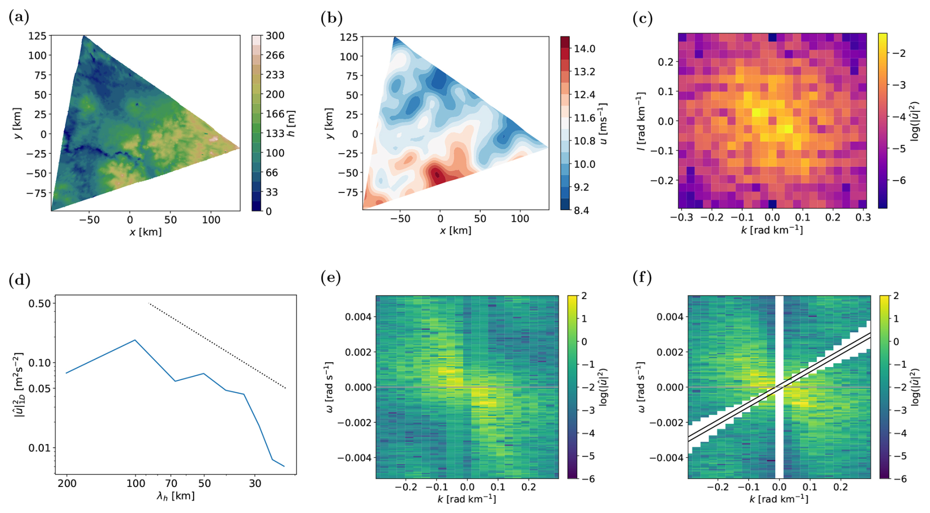
Figure 2 Illustration of the methodology on a randomly selected triangle near Kanin Peninsula. (a) Topography at the triangular subdomain. (b) Original zonal velocity field. (c) Horizontal spectrum computed from the zonal velocity in panel (b). (d) 1D spectrum computed from the horizontal spectrum in panel (c), indicating the spectral slope close to −5/3 (slanted line). (e) Cross-section of the spatiotemporal spectrum for l=0 obtained by the Fourier transform of the time series of horizontal spectra. (f) Cross-section of the spectrum from panel (e) projected onto the GW mode with m>0, displayed again for l=0, the two slanted lines denote the lines $\widehat{\mathit{\omega }}=\pm \left|f\right|$.

If we take 24 h evolution of the horizontal spectra at the triangular subdomain and apply the Fourier transform in time, we arrive at the 3D spectrum with a cross-section for l=0 shown in Fig. 2e. There are again large values of spectral amplitude for long wavelengths and long periods, which is consistent with previous studies (e.g., Subba Reddy et al., 2005). The quantity shown in the figure is the spectral density of the zonal velocity perturbation, the spectrum of kinetic energy density would be, however, very similar. The spectrum in Fig. 2e is symmetric with respect to the change of sign $k,l,\mathit{\omega }$ → $-k,-l,-\mathit{\omega }$, which is a general property of the Fourier transform of real fields. The low values for $k=l=\mathrm{0}$ are caused by the deplaning of the data.

The 3D spectrum is then projected to GW modes using the projection described in Eq. (17) and limited to the range of intrinsic frequencies described by Eqs. (18) and (19). The spectrum projected onto the GW mode with positive wavenumber is shown in Fig. 2f. The basic structure of the spectrum is similar to that of the original 3D spectrum. However, due to the projection, the exact symmetry of Fig. 2e is no longer present. Since the spectrum is now a function of the vertical wavenumber through the selection of the gravity mode as well, there is a similar symmetry with respect to the change of sign $k,l,m,\mathit{\omega }\to -k,-l,-m,-\mathit{\omega }$. This implies that the full spectrum for m>0 already contains all information, since the projection to the other mode can be obtained by the coordinate transformation, which makes it sufficient to study only the mode with positive vertical wavenumber. The representation by positive m and both signs of frequency and horizontal wavenumber is chosen to simplify discussion of the results. Other representations, such as using positive frequency and both signs of the wavenumbers, carry the same information and it is possible to switch to them using the symmetry of the spectra.

The projected spectrum is divided by two planes, $\widehat{\mathit{\omega }}=\pm f$, represented in Fig. 2f as the two slanted lines. As linear GW theory implies the limit on intrinsic frequency $\left|f\right|<\widehat{\mathit{\omega }}$ (Eq. 18), there cannot be GWs between those two planes, hence the empty spots in the plot. Furthermore, since the sign of the vertical group velocity component of the GW corresponds to the sign of $-m/\widehat{\mathit{\omega }}$, we can see that the part of the spectrum where the intrinsic frequency is positive represents downward propagating waves and vice versa. In Fig. 2f, this means that the parts of the plot above and below the slanted lines are downward and upward propagating waves, respectively. By looking at the plot, it can be therefore noted that at least for the selected subdomain, altitude and day, the upward propagating waves are stronger compared to the downward propagating waves. Numerically, upward propagating waves in this case cause 58 % of the energy of the zonal velocity $\int |\widehat{u}{|}^{\mathrm{2}}\mathrm{d}k\mathrm{dl}\mathrm{d}\mathit{\omega }$. However, please note that this percentage is for the selected subdomain only. The global distribution of the percentage of upward propagating wave energy will be presented in Sect. 3.2.

Another region of missing values in the projected spectrum is the column of $k=l=\mathrm{0}$, which also does not describe GWs, as the dispersion relation for these wavenumbers does not result in a real vertical wavenumber. Finally, the blank space in Fig. 2f is also around the $\widehat{\mathit{\omega }}=\pm f$ planes for larger k and l. These values are removed because the vertical wavenumber given by the dispersion relation is in this region higher than what could be present according to the vertical resolution of the model.

The same plots for another subdomain are shown in Fig. 3. This subdomain lies on the Scandinavian Peninsula at 62° N and 7° E, which is known for exciting orographic GWs and thus provides a potentially more complex wave field. This is directly visible in Fig. 3b, where there are more small-scale perturbations of the wind compared to Fig. 2b for the previous subdomain. As in the previous case, the direction of the perturbations is visible in the directionality of the horizontal spectrum in Fig. 3c. The horizontal spectrum is more anisotropic compared to the previous case, although the 1D spectrum in Fig. 3d still points to a decreasing magnitude for decreasing wavelengths, with the slope oscillating around the slope −5/3.

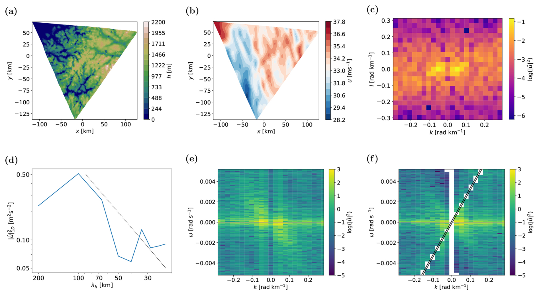
Figure 3 Illustration of the methodology on a triangle at Scandinavian Peninsula. (a–f) As in Fig. 3.

The most noticeable difference between the spectra in the two subdomains is visible in the 3D spectra, especially after the GW projection (Fig. 3f). For the second subdomain, we do not see that the spectral values decrease with frequency and zonal wavenumber as in Fig. 2f due to much higher values around the extrinsic frequency ω=0. This means that the majority of the waves on the subdomain are stationary, which is typical for orographic GWs. Again, we see higher values in the right part of Fig. 3f, suggesting the dominant upward propagation of the waves. In this case, the percentage of energy for the upward propagating waves reaches 82 %, which is reasonable for the waves generated mostly by the orography.

3.2 Global distribution of gravity waves

The GW spectra presented in the previous section are informative about the wave type in individual subdomains. Now, we will extend our analysis to the global imprint of GWs.

In Fig. 4a, we show the distribution of the total energy computed from the GW spectra using Eq. (20) for a single day of the simulation. The most significant areas with high energy are the orographic regions (e.g., Andes, Rocky Mountains, Alaska Range, Greenland, Island or Himalayas) and the regions of the Southern Hemisphere connected to the subtropical convection. Apart from that, we also see GWs with other sources in the mid-latitudes and above the equator. The magnitude of the energy is, however, much weaker – note the logarithmic axis of the plot.

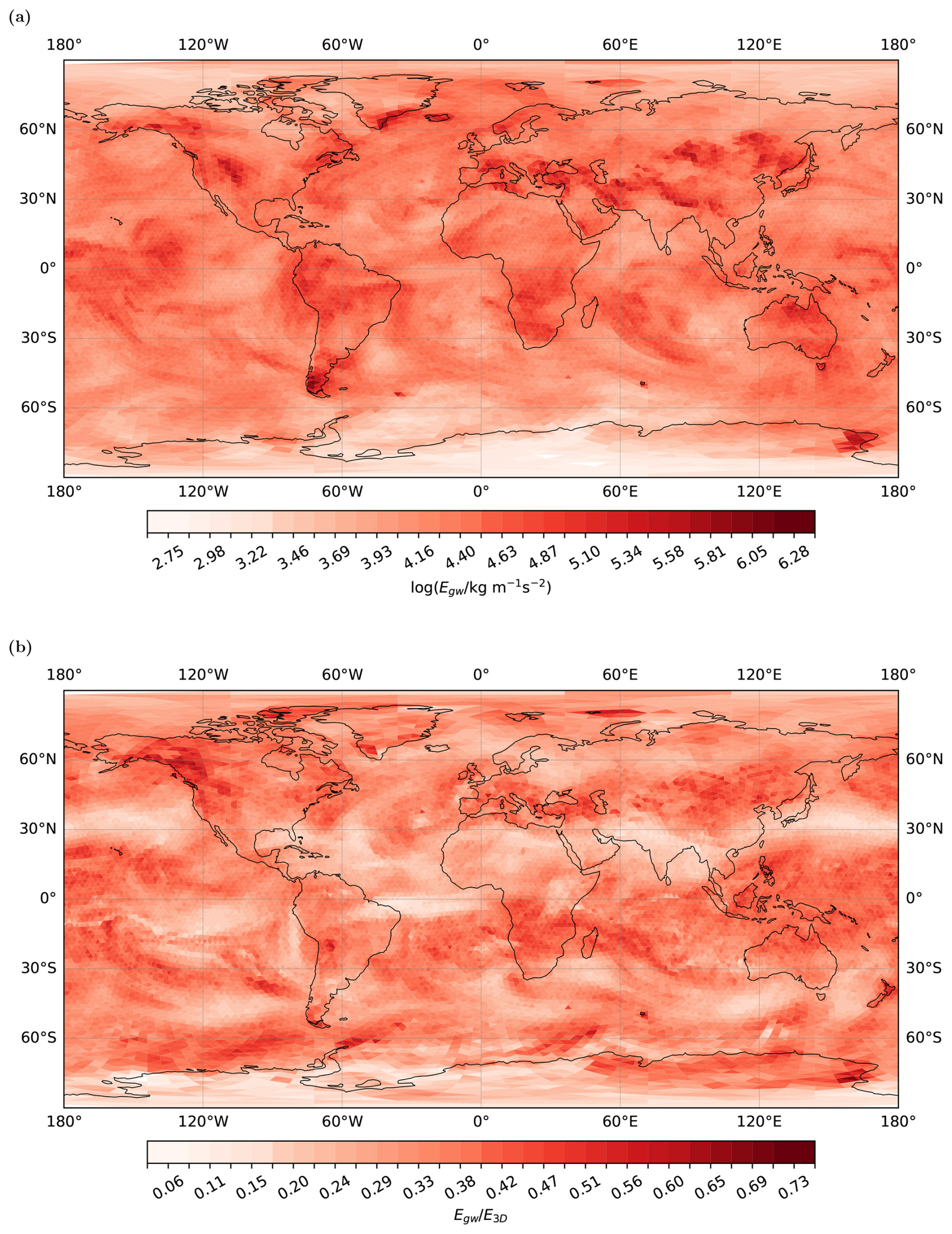
Figure 4 Global distribution of GWs on 23 January 2020. (a) Total energy of GW spectra, as obtained by the GW projection, visualising particularly GW hotspots above orography, and also weaker GW signal in mid-latitudes and above the equator. (b) Fraction between the projected GW part and the 3D spectrum of total energy, describing the effect of GW projection compared to the removal of larger scales.

The energy can also be computed from the 3D spectra before the GW projection. Although such spectra should in principle describe all processes in the data, we again see only small scales because the size of the domains being around 200 km at most. Therefore, the global distribution of the energy is very similar to the distribution in Fig. 4a, mainly highlighting regions with orography.

The fraction between the energy computed from the GW spectra and the energy computed from the total 3D spectra is visualised in Fig. 4b. In the plot, we can distinguish between regions where the GW projection removes the majority of the spectra (low values of the fraction) and where the large part of the spectra projects well onto the GW modes (high values). The most noticeable result is the decrease in the spectra in the subtropical jet regions, especially in the Northern Hemisphere. At these regions, the jet introduces wind gradients that result in larger Fourier coefficient amplitudes at the subdomains, increase the 3D spectrum, but do not describe the GWs. However, the largest ratio between the energies is in the Alaska Range or Franz Josef Land. Nevertheless, the fraction is still not one, which, especially because of the logarithmic character of the gravity wave energy, means that we are discarding a noticeable part of the spectra by the GW projection. Apart from the wind perturbations at the subdomains that are not caused by GWs, the GW projection would also dismiss nonlinearities due to the applied linearized theory. This could be the reason for the decreased amplitudes after the projection, especially for the stronger orographic GWs.

As shown in Sect. 3.1, the GW projection method also allows us to distinguish between upward and downward propagating waves. For the day shown in Fig. 4a, the fraction of total energy of the upward propagating waves is visualized in Fig. 5. At most places, 70 %–80 % of the wave energy propagates upward, highlighting the importance of tropospheric wave sources. A lower percentage is present in two regions, where the values decrease even below 50 %. First, the fraction is generally lower above the tropical Pacific and Atlantic ocean. This is likely connected to the fact that the tropopause is in the tropics higher than the studied altitude and the spectrum can therefore be dominated by convective GWs coming from above. Second, the figure shows significant downward propagating waves at the northern-hemispheric polar regions, especially above the Chukotka region, possibly originating at the edge of the polar vortex (Vadas et al., 2023) in the absence of strong tropospheric sources.

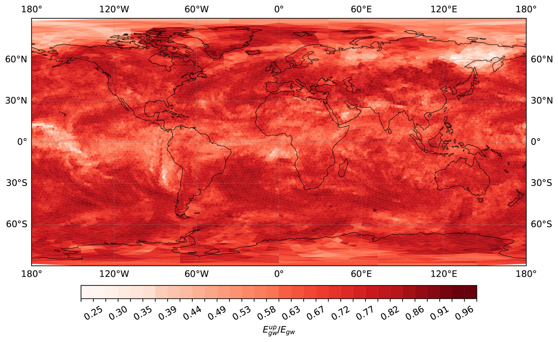
Figure 5 Percentage of upward propagating waves on 23 January 2020, described by the total energy of GWs.

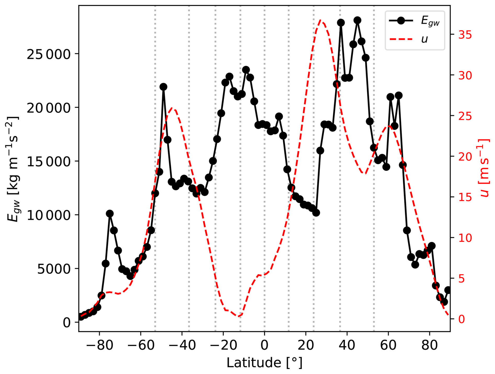
In Fig. 6, we show the zonal mean distribution of the energy from Fig. 4a. The orographical GW hotspots are clearly visible as the strong peaks in the plot. The gravity wave energy is higher at the Northern Hemisphere, since the wind is stronger at the winter hemisphere (see the red line in the figure). Although the individual hotspots in the Northern Hemisphere produce lower GW energy compared to the southern Andes region, there is more orography in the Northern Hemisphere, increasing the total zonal-averaged energy. An interesting region is the band southward from the equator, where the zonal mean zonal wind is close to zero. In that region, there is no distinct orography. The local maximum of the GW energy is therefore most likely linked to the convectively generated GWs above the subtropics and near the Intertropical Convergence Zone (ITCZ).

Figure 6 Zonal mean of GW energy and the zonal mean zonal wind for the first day of the data. The plot reveals higher GW energy at the regions with orography and southward from the equator. Vertical lines are marking the latitude groups introduced in Sect. 3.3.

3.3 Spectra variability

Lastly, we will look at how the shape of the spectrum differs between the subdomains, which is a key factor in assessing how simplified a GW parametrisation can be. Due to the meridionally dependent wind structure and distribution of GW sources such as orography or convection, we anticipate differences among latitudes. Therefore, we divide the subdomains into 10 groups of 2048 subdomains based on latitude. As the equatorial region contains significantly more grid cells along the parallel lines, the groups closer to the equator are narrower compared to the groups closer to the poles. The latitudinal ranges for these groups are listed in Table 1 and visualised in Fig. 6.

Table 1 Latitude ranges for groups at the Northern Hemisphere. Southern hemispheric groups are denoted in the brackets.

In each group, we interpolate the GW spectra of the wave action density onto a constant klm grid and perform principal component analysis (PCA) to simplify these spectra. Based on the vertical wavenumber values computed from the dispersion relation, we select 12 positive and 12 negative vertical wavenumbers logarithmically spaced between the values corresponding to the vertical wavelengths 2.7 and 30.4 km. The PCA is applied $\log (\stackrel{\mathrm{̃}}{\mathcal{N}}+\mathrm{1})$ for $\stackrel{\mathrm{̃}}{\mathcal{N}}=\mathcal{N}/$(1 kg m² s⁻¹) instead of just 𝒩, as this focuses the analysis on the wavelengths for which the wave action density is largest while allowing changes in the order of magnitude. To have a sufficient number of samples for the PCA (2048 subdomains for 7 independent daily spectra), we reduced the number of points in k and l direction by half, so that the resulting klm grid contains approximately 2600 data points for each spectrum.

We ask the following questions:

• Are there some differences in averages or principal components between the groups?

• How many principal components are needed in the individual groups?

The first question gives an estimate on how the spectra launched by GW parametrisations should look like for different latitudes. The second question assesses the spatial variability of the spectra within the latitude ranges and the possibility to compress the spectra by PCA, so that the parametrisations can more easily encompass this variability.

First, we will describe the average spectrum of the wave action density. In general, the wave action density is maximal for long horizontal wavelengths and short vertical wavelengths (Fig. 7). The wave action density maxima are slightly asymmetrical, with higher values for purely meridional waves compared to the solely zonal ones with the same horizontal wavelength.

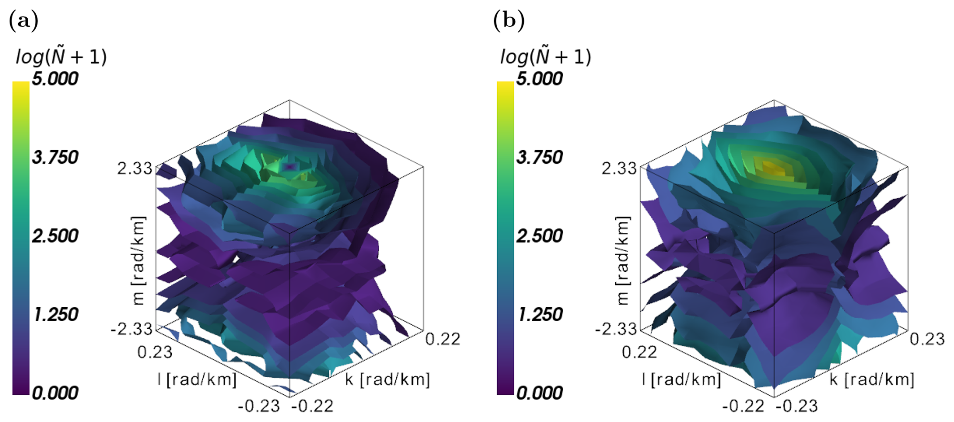
Figure 7 Average wave action density in two different groups. (a) Group 1. (b) Group 4. For the equatorial group 4, the spectrum is more symmetrical.

When comparing the ten latitude groups, two different types of spectra are observed. For groups 4, 5 and 6, the spectra are relatively symmetric with respect to k and l (see group 4 in Fig. 7b). In contrast, the remaining groups are skewed in the direction of negative k (Fig. 7a, visible on the contours with lower wave action density). This is likely caused by the direction of the mean wind. The wind at the studied altitude at the higher latitudes is purely zonal, which influences the range of intrinsic frequencies observed in the data through the $k\stackrel{\mathrm{‾}}{u}$ term in the definition of intrinsic frequency. For the positive zonal wind $\stackrel{\mathrm{‾}}{u}>\mathrm{0}$ and positive zonal wavenumbers k>0, the intrinsic frequencies $\widehat{\mathit{\omega }}$ decrease with increasing zonal wavenumber. This decrease then causes an increase of the vertical wavenumber following Eq. (11). As a result, there are not enough subdomains with short zonal wavelength and long vertical wavelengths, causing the decrease in the values in the plot region.

Additionally, the skewness of the spectrum can be qualitatively explained by the distinct propagation behaviour of GWs from different sources. Since the propagation direction of orographic GWs is always generally opposite to the wind, more energy would propagate westward in the regions with orography and westerly winds. On the other hand, the mechanism of generation of convective GWs does not directly enforce a propagation direction, possibly leading to a more symmetrical spectrum.

The shape of principal components (PCs) from the PCA is also strongly influenced by the shape of the wave action density spectrum. The first three PCs for groups 1 and 4 are shown in Fig. 8. The equatorial cases with symmetric spectrum (group 4 in Fig. 8d–f) provide PCs with the most comprehensible meaning. The first two PCs determine the direction of the zonal and meridional wavenumber, respectively. The third component further modifies the distribution of the wave action density described by the second component. A similar representation of the first modes is also present for the other equatorial groups 5 and 6.

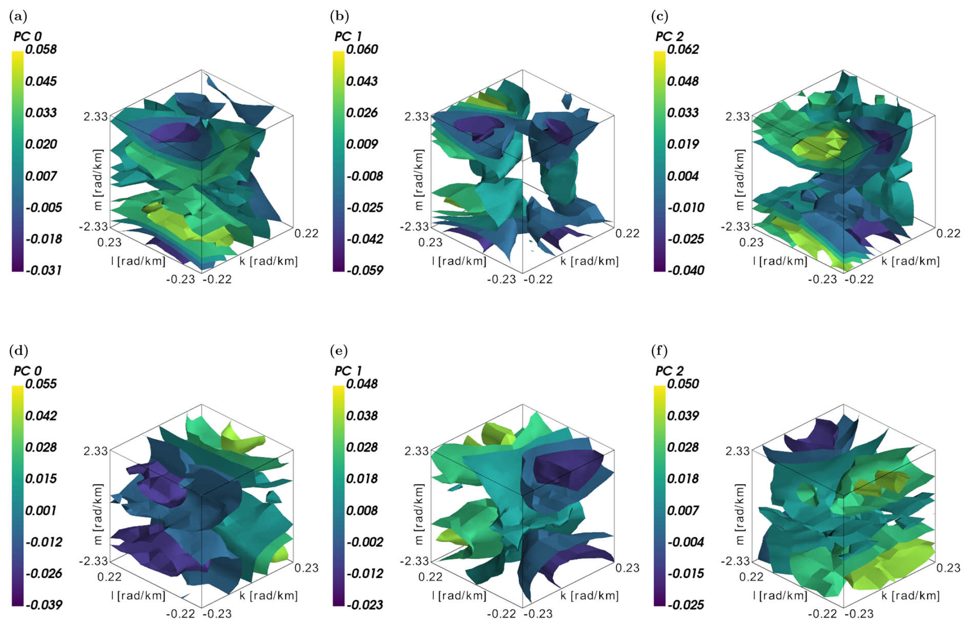
Figure 8 Individual principal components 0,1 and 2 (columns) of wave action density in groups 1 (top) and 4 (bottom). The first few components mainly estimate the major structure in zonal, meridional and vertical directions, which is noticeable especially for group 4.

Regarding the extratropical groups, the situation is less clear, since the reduced number of available data in the regions of positive k effectively increases the variance there, which enforces the first few PCs to describe these spectral regions. However, in Fig. 8a–b, parts of the PCs modifying the horizontal spectra in the north-west and north-east directions can still be observed. Similar, usually oblique, horizontal directions are also observable in the remaining groups (not shown).

Most importantly, the PCA is effective in approximating the final shape of the spectra. Figure 9 shows how many PCs we need to explain a given percentage of variance for the individual groups. To obtain 80 % of the spectra variance, 50 PCs are sufficient for the majority of the groups. If the aim is to obtain 95 % of the variance, about 400 PCs are needed, which still means decreasing the number of values necessary to describe the spectra by a factor of 5.

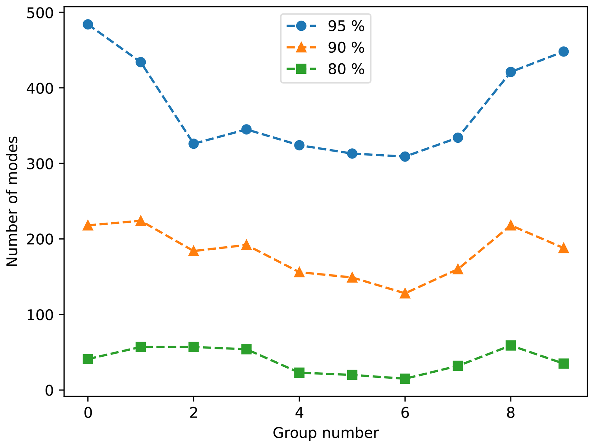
Figure 9 Percentage of variability explained by a reduced number of modes. Generally, a relatively low number of PCs is needed to reconstruct most of the spectrum variability. Higher number of components is needed in the mid-latitudes.

Finally, the complexity of the GW spectra represented by the efficiency of the PCA in Fig. 9 also depends on the latitude. If we are interested in a basic shape of the spectra (80 % of the variance), the spectra show more complex structure in the middle latitudes, although they are relatively simpler at the poles and at the equatorial groups. The higher complexity in the mid-latitudes is most likely connected to the more complex, strong circulation caused by the subtropical jet. This is also in coherence with the fact that more PC are needed in the northern, winter hemisphere, where the circulation is also stronger. It should be noted here that the complexity does not depend on the strength of the GW field, as illustrated in Fig. 6, but rather on the zonal mean zonal wind. On the other hand, if the aim is to capture higher percentage of the variability, approximation of the polar and mid-latitude regions becomes more demanding. This implies that the polar group has highly variable spectra, although the general structure is likely determined by the wind.

The possible simplification of a selected spectrum from groups 1 and 4 using a limited number of modes is visualised in Fig. 10. When approximated with 20 PCs only (first column), the shape of the spectrum is already reasonably captured for both the examples. It is however smoother compared to the original spectrum, which can be improved by considering more PCs (second column for 200 PCs). The coarseness of the spectrum from group 1 complicates the approximation using PCA. Although the reconstructed spectra for both the groups do not look exactly the same as the original spectra even for the 200 PCs, the basic structure is preserved already by the first 20 modes and they could provide a reasonable approximation.

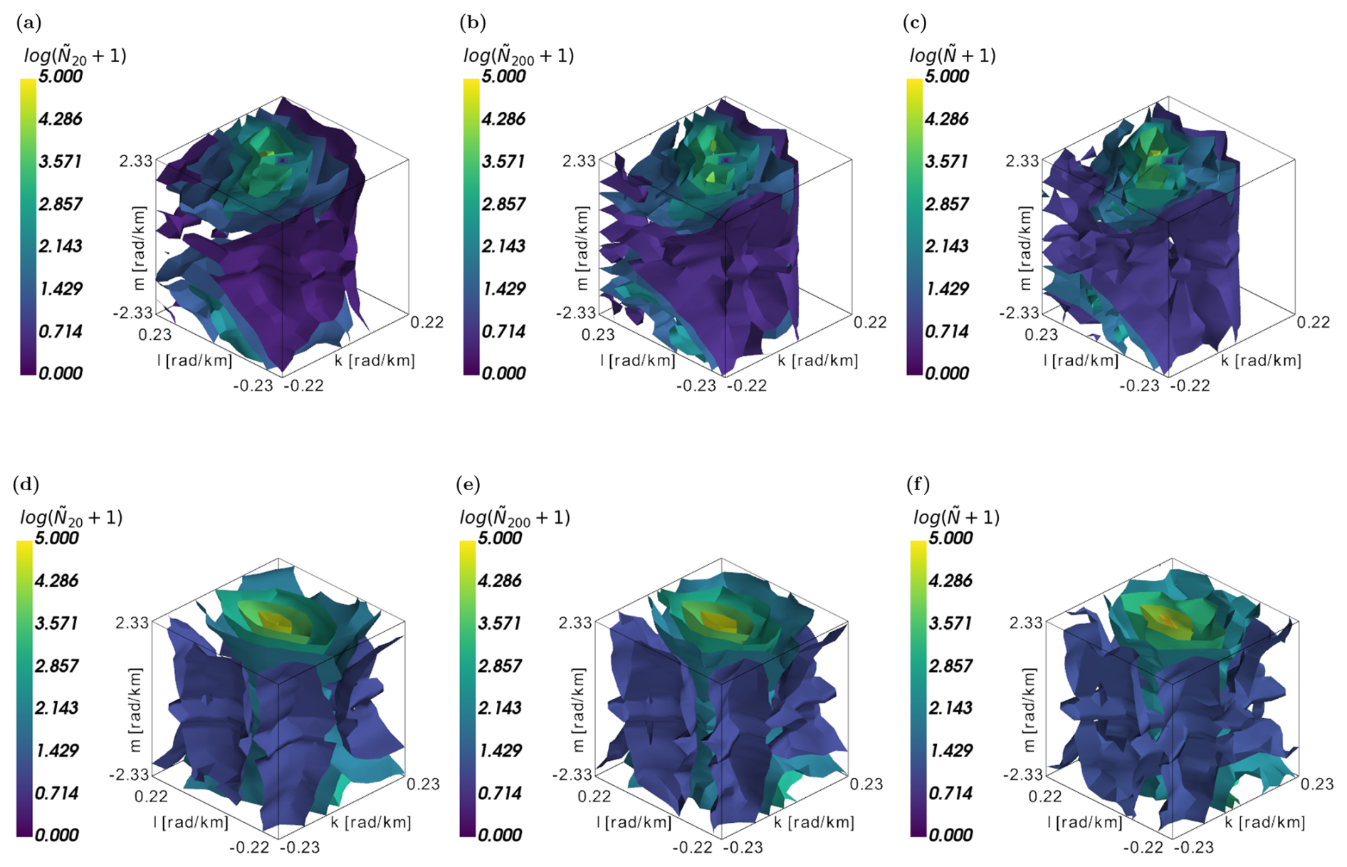
Figure 10 Representation of a random single spectrum (third column) from groups 1 (top) and 4 (bottom) by 20 (first column) and 200 PCs (second column). With the 200 components, the main structure of the 3D spectrum is well represented, especially for the more symmetric case of group 4.

4 Discussion and conclusion

This study presents the variability of local gravity wave spectra at different geographical locations. To obtain the results, a novel methodology for spectrum computation and GW separation is applied. In terms of spectrum computation, horizontal interpolation is avoided by proceeding on a triangular grid. As we are working with the original triangular model grids, the resulting spectra describe the dynamics that would not be resolved by a low-resolution simulation, giving a direct interpretation to the results. Additionally, using data directly on the model grid avoids interpolation errors that usually lead to underestimation of the spectra (Mossad et al., 2024). Although similar fitting procedures were used in previous studies (VanderPlas and Ivezic, 2015), Chew et al. (2024) observed that they introduce errors in the amplitudes. However, since atmospheric quantities have mostly power-law spectra and we focus on small wavenumbers, our approach resembles a more precise method introduced by Chew et al. (2024, Constrained Spectral Approximation method), where the procedure is iterated for the wavenumbers with the largest amplitudes, which reduces the error in our results.

In order to isolate the GW contribution, the spectrum computation is followed by a projection to GW modes. The method is similar to the projection applied in Borchert et al. (2014), where the data are projected onto an orthonormal basis defined by a geostrophic mode, two gravity wave modes and a remaining part. Compared to the procedure in this study, there are some differences. First, we did not use the Boussinesq approximation, which makes the approach applicable for higher altitudes. Although this also allows sound waves among the resulting modes in principle, they cannot be analysed here because the sound waves are dampened in the model and due to the low temporal resolution of the data. Second, since we were analysing data at a single altitude only, we do not get the spectra in the wavenumber klm space directly from the GW projection as in Borchert et al. (2014), but they are described rather by horizontal wavenumbers k, l and frequency ω. For dedicated experiments which are saved at short time steps, a $k,l,\mathit{\omega }$ analysis is the better choice as the frequency is less subject to changes by, e.g., refraction compared to the vertical wavenumber. A limitation of the procedure is the necessity for using data with a short output timestep, increasing the disc-space requirements. The 10 min output frequency applied in our case is at the limit of what is needed to capture the dominant period of convective GWs (Lane et al., 2001).

In GW research, GW perturbations are often separated from model data by removing larger scales, using a spectral cutoff (e.g., Sun et al., 2023; Gupta et al., 2024; Dörnbrack, 2024). Here, we apply the GW projection after the removal of large-scale motions. As a result, we can compare the efficiency of scale separation as a GW filtering method. We observed that the scale-based filtering results in similar GW signature, with an overestimation of GWs near the subtropical jet streams. The effectiveness of a horizontal filtering of GWs is in accordance with the work of Strube et al. (2020) for higher altitudes.

The advantage of our methodology, compared to simple scale-based filters, is also the possibility of a detailed study of the GW spectra. For example, the separation between the parts of the spectra with upward and downward propagating waves can be useful in future GW studies to distinguish whether the waves were generated in lower or upper vertical levels. Furthermore, the shape of the 3D GW spectra reveals the strength of the stationary part of the waves, which can help attribute the GWs to the wave sources. Such analysis is planned for a future study.

We analyse the variability of the spectra at different geographical bands. We see that the basic structure of the spectra is complex in the regions with strong zonal winds and the spectra are more variable in the polar regions. The results further suggest that the GW spectra can be well approximated by a limited number of GW modes. This is potentially useful for GW parametrisations, as it simplifies the spectra to be simulated by the models.

A certain limitation of this study is the restriction of the analysis to a single week due to computational limits. Thanks to the high number of subdomains with various atmospheric conditions in both hemispheres, we can however consider our results to be representative when related, for example, to the zonal wind.

In general, the study analyses the variability of GW spectra with a novel methodology in an ICON simulation, with the results providing valuable insights for refining GW parameterisations and guiding future investigations of GWs. Next, we plan to apply these findings to better characterise individual GW sources. As part of the analysis, GW sources in different areas will be identified using data describing topography or convection and spectrum shapes will be connected to those sources by machine learning techniques.

Appendix A: Derivation of dispersion relation and gravity wave projection

To derive the general dispersion relation for acoustic-gravity waves, we will start with the transformed set of linearised equations of motion, entropy equation and the continuity equation (as derived in Achatz, 2022, Chap. 10), assuming the adiabaticity of the wave perturbations,

$$\begin{array}{}\text{(A1)}& {\displaystyle }-\mathrm{i}\widehat{\mathit{\omega }}\stackrel{\mathrm{̃}}{u}-f\stackrel{\mathrm{̃}}{v}& {\displaystyle }=-\mathrm{i}k\stackrel{\mathrm{̃}}{p}{\displaystyle \frac{c_s}{{\mathit{\rho }}_{\mathrm{0}}}},\text{(A2)}& {\displaystyle }-\mathrm{i}\widehat{\mathit{\omega }}\stackrel{\mathrm{̃}}{v}+f\stackrel{\mathrm{̃}}{u}& {\displaystyle }=-\mathrm{i}l\stackrel{\mathrm{̃}}{p}{\displaystyle \frac{c_s}{{\mathit{\rho }}_{\mathrm{0}}}},\text{(A3)}& {\displaystyle }-\mathrm{i}\widehat{\mathit{\omega }}\stackrel{\mathrm{̃}}{w}& {\displaystyle }=\left({\displaystyle \frac{\mathrm{1}}{H_{\mathit{\theta }}}}-{\displaystyle \frac{\mathrm{1}}{\mathrm{2}H}}-\mathrm{i}m\right)\stackrel{\mathrm{̃}}{p}{\displaystyle \frac{c_s}{{\mathit{\rho }}_{\mathrm{0}}}}+N\stackrel{\mathrm{̃}}{b},\text{(A4)}& {\displaystyle }-\mathrm{i}\widehat{\mathit{\omega }}\stackrel{\mathrm{̃}}{b}+N\stackrel{\mathrm{̃}}{w}& {\displaystyle }=\mathrm{0},\text{(A5)}& {\displaystyle }-\mathrm{i}\widehat{\mathit{\omega }}{\displaystyle \frac{\stackrel{\mathrm{̃}}{p}}{c_s{\mathit{\rho }}_{\mathrm{0}}}}& {\displaystyle }=-\mathrm{i}k\stackrel{\mathrm{̃}}{u}-\mathrm{i}l\stackrel{\mathrm{̃}}{v}-\left({\displaystyle \frac{\mathrm{1}}{H_{\mathit{\theta }}}}-{\displaystyle \frac{\mathrm{1}}{\mathrm{2}H}}+\mathrm{i}m\right)\stackrel{\mathrm{̃}}{w}\end{array}$$

for $\stackrel{\mathrm{̃}}{u}$, $\stackrel{\mathrm{̃}}{v}$, $\stackrel{\mathrm{̃}}{w}$, $\stackrel{\mathrm{̃}}{p}$ and $\stackrel{\mathrm{̃}}{b}$ defined from the wind, pressure and buoyancy perturbations u^′, v^′, w^′, p^′ and b^′ as

$$\begin{array}{}\text{(A6)}& \left(\begin{array}{c}{u}^{\prime }\\ v^{\prime }\\ w^{\prime }\\ b^{\prime }\\ p^{\prime }\end{array}\right)=\int \mathrm{d}k\mathrm{d}l\mathrm{d}m\mathrm{d}\mathit{\omega }{e}^{\mathrm{i}(kx+ly+mz-\mathit{\omega }t)}\left(\begin{array}{c}\frac{\stackrel{\mathrm{̃}}{u}}{\sqrt{\stackrel{\mathrm{‾}}{\mathit{\rho }}/{\mathit{\rho }}_{\mathrm{0}}}}\\ \frac{\stackrel{\mathrm{̃}}{v}}{\sqrt{\stackrel{\mathrm{‾}}{\mathit{\rho }}/{\mathit{\rho }}_{\mathrm{0}}}}\\ \frac{\stackrel{\mathrm{̃}}{w}}{\sqrt{\stackrel{\mathrm{‾}}{\mathit{\rho }}/{\mathit{\rho }}_{\mathrm{0}}}}\\ \frac{\stackrel{\mathrm{̃}}{b}N}{\sqrt{\stackrel{\mathrm{‾}}{\mathit{\rho }}/{\mathit{\rho }}_{\mathrm{0}}}}\\ \stackrel{\mathrm{̃}}{p}{c}_s\sqrt{\stackrel{\mathrm{‾}}{\mathit{\rho }}/{\mathit{\rho }}_{\mathrm{0}}}\end{array}\right),\end{array}$$

with the same notation as in Sect. 2. This system can be rewritten into the matrix form

$$\begin{array}{}\text{(A7)}& -\mathrm{i}\widehat{\mathit{\omega }}\mathit{Z}=\mathbf{M}\mathit{Z}\end{array}$$

for $Z=(\stackrel{\mathrm{̃}}{u},\stackrel{\mathrm{̃}}{v},\stackrel{\mathrm{̃}}{w},\stackrel{\mathrm{̃}}{b},\stackrel{\mathrm{̃}}{p}/{\mathit{\rho }}_{\mathrm{0}})$ and matrix

$$\begin{array}{}\text{(A8)}& \begin{array}{rl}& \mathbf{M}=\\ & \left(\begin{array}{ccccc}\mathrm{0}& f& \mathrm{0}& \mathrm{0}& -\mathrm{i}k{c}_s\\ -f& \mathrm{0}& \mathrm{0}& \mathrm{0}& -\mathrm{i}l{c}_s\\ \mathrm{0}& \mathrm{0}& \mathrm{0}& N& \left(\frac{\mathrm{1}}{H_{\mathit{\theta }}}-\frac{\mathrm{1}}{\mathrm{2}H}-\mathrm{i}m\right)c_s\\ \mathrm{0}& \mathrm{0}& -N& \mathrm{0}& \mathrm{0}\\ -\mathrm{i}k{c}_s& -\mathrm{i}l{c}_s& -\left(\frac{\mathrm{1}}{H_{\mathit{\theta }}}-\frac{\mathrm{1}}{\mathrm{2}H}+\mathrm{i}m\right)c_s& \mathrm{0}& \mathrm{0}\end{array}\right).\end{array}\end{array}$$

Therefore, we have an eigenvalue problem that has a non-zero solution if and only if it holds $\det (\mathrm{i}\widehat{\mathit{\omega }}\mathit{I}+\mathbf{M})=\mathrm{0}$, where I is the identity matrix. The determinant in the condition can be evaluated, which results in the following equality

$$\begin{array}{}\text{(A9)}& \begin{array}{rl}-\mathrm{i}\widehat{\mathit{\omega }}[& (N^{\mathrm{2}}-{\widehat{\mathit{\omega }}}^{\mathrm{2}})\left({\widehat{\mathit{\omega }}}^{\mathrm{2}}-f^{\mathrm{2}}-c_s^{\mathrm{2}}(k^{\mathrm{2}}+l^{\mathrm{2}})\right)\\ & +({\widehat{\mathit{\omega }}}^{\mathrm{2}}-f^{\mathrm{2}})\left({\left({\displaystyle \frac{\mathrm{1}}{H_{\mathit{\theta }}}}-{\displaystyle \frac{\mathrm{1}}{\mathrm{2}H}}\right)}^{\mathrm{2}}+m^{\mathrm{2}}\right)c_s^{\mathrm{2}}]=\mathrm{0}.\end{array}\end{array}$$

The equality is true if $\widehat{\mathit{\omega }}=\mathrm{0}$ or if

$$\begin{array}{}\text{(A10)}& m^{\mathrm{2}}+{\left({\displaystyle \frac{\mathrm{1}}{H_{\mathit{\theta }}}}-{\displaystyle \frac{\mathrm{1}}{\mathrm{2}H}}\right)}^{\mathrm{2}}=-{\displaystyle \frac{N^{\mathrm{2}}-{\widehat{\mathit{\omega }}}^{\mathrm{2}}}{c_s^{\mathrm{2}}}}+(k^{\mathrm{2}}+l^{\mathrm{2}}){\displaystyle \frac{N^{\mathrm{2}}-{\widehat{\mathit{\omega }}}^{\mathrm{2}}}{{\widehat{\mathit{\omega }}}^{\mathrm{2}}-f^{\mathrm{2}}}}.\end{array}$$

Further, using the definitions $H_{\mathit{\theta }}=H{c}_p/R$, $R=c_p-c_v$, $H=R\stackrel{\mathrm{‾}}{T}/g$, $c_s^{\mathrm{2}}=R\stackrel{\mathrm{‾}}{T}{c}_p/c_v$ and $N^{\mathrm{2}}=g/H_{\mathit{\theta }}$, it can be shown that

$$\begin{array}{}\text{(A11)}& N^{\mathrm{2}}+c_s^{\mathrm{2}}{\left({\displaystyle \frac{\mathrm{1}}{H_{\mathit{\theta }}}}-{\displaystyle \frac{\mathrm{1}}{\mathrm{2}H}}\right)}^{\mathrm{2}}={\displaystyle \frac{c_s^{\mathrm{2}}}{\mathrm{4}{H}^{\mathrm{2}}}}.\end{array}$$

Finally, this can be substituted to the previous equation to give

$$\begin{array}{}\text{(A12)}& m^{\mathrm{2}}=k_h^{\mathrm{2}}{\displaystyle \frac{N^{\mathrm{2}}-{\widehat{\mathit{\omega }}}^{\mathrm{2}}}{{\widehat{\mathit{\omega }}}^{\mathrm{2}}-f^{\mathrm{2}}}}+{\displaystyle \frac{{\widehat{\mathit{\omega }}}^{\mathrm{2}}}{c_s^{\mathrm{2}}}}-{\displaystyle \frac{\mathrm{1}}{\mathrm{4}{H}^{\mathrm{2}}}}\end{array}$$

for $k_h^{\mathrm{2}}=k^{\mathrm{2}}+l^{\mathrm{2}}$, which is the dispersion relation for acoustic-gravity waves (Eq. 11). When inverted to give dependence of intrinsic frequency on wavenumbers (Eq. B1), it provides us with two dispersion relations for gravity waves and two dispersion relations for sound waves.

Since the intrinsic frequencies $\widehat{\mathit{\omega }}$ are eigenvalues of the system (Eq. A7) with an anti-hermitian matrix M, the corresponding eigenvectors form orthogonal subspaces. This property is used in the methodology when we project the spectrum onto the GW subspaces, and it also explains the form of the scalar product used for the projection: When considering the scaling between the Fourier amplitudes and the variables with tilde in Eq. (A6), the inner product applied on a vector of the form $\mathit{Z}=(\stackrel{\mathrm{̃}}{u},\stackrel{\mathrm{̃}}{v},\stackrel{\mathrm{̃}}{w},\stackrel{\mathrm{̃}}{b},\stackrel{\mathrm{̃}}{p}/{\mathit{\rho }}_{\mathrm{0}})$ in Euclidean space translates to the inner product described by Eq. (16).

Appendix B: Intrinsic frequency limits for gravity waves

The general form of the dispersion relation for both gravity and sound waves (Achatz, 2022) can be computed by solving Eq. (A12) for ${\widehat{\mathit{\omega }}}^{\mathrm{2}}$ as

$$\begin{array}{}\text{(B1)}& \begin{array}{rl}{\widehat{\mathit{\omega }}}_{\mathrm{sw},\mathrm{gw}}^{\mathrm{2}}=& {\displaystyle \frac{\mathrm{1}}{\mathrm{2}}}\left[f^{\mathrm{2}}+c_s^{\mathrm{2}}\left(k_h^{\mathrm{2}}+m^{\mathrm{2}}+{\displaystyle \frac{\mathrm{1}}{\mathrm{4}{H}^{\mathrm{2}}}}\right)\right]\\ & \pm \sqrt{\begin{array}{c}\frac{\mathrm{1}}{\mathrm{4}}{\left[f^{\mathrm{2}}+c_s^{\mathrm{2}}\left(k_h^{\mathrm{2}}+m^{\mathrm{2}}+\frac{\mathrm{1}}{\mathrm{4}{H}^{\mathrm{2}}}\right)\right]}^{\mathrm{2}}\\ -c_s^{\mathrm{2}}\left[N^{\mathrm{2}}{k}_h^{\mathrm{2}}+f^{\mathrm{2}}\left(m^{\mathrm{2}}+\frac{\mathrm{1}}{\mathrm{4}{H}^{\mathrm{2}}}\right)\right]\end{array}},\end{array}\end{array}$$

with the notation introduced in Sect. 2. For sufficiently large $k_h^{\mathrm{2}}+m^{\mathrm{2}}+\mathrm{1}/\mathrm{4}{H}^{\mathrm{2}}$, the previous equation with the negative sign before the square root translates to the standard dispersion relation for GWs

$$\begin{array}{}\text{(B2)}& {\widehat{\mathit{\omega }}}_{\mathrm{gw}}^{\mathrm{2}}\approx {\displaystyle \frac{N^{\mathrm{2}}{k}_h^{\mathrm{2}}+f^{\mathrm{2}}\left(m^{\mathrm{2}}+\mathrm{1}/\mathrm{4}{H}^{\mathrm{2}}\right)}{k_h^{\mathrm{2}}+m^{\mathrm{2}}+\mathrm{1}/\mathrm{4}{H}^{\mathrm{2}}}}.\end{array}$$

Equation (B1) with the positive sign describes the sound waves.

The goal here is to find limits on the intrinsic frequency of GWs, such that ${\widehat{\mathit{\omega }}}_{\mathrm{gw},\min }^{\mathrm{2}}\le {\widehat{\mathit{\omega }}}_{\mathrm{gw}}^{\mathrm{2}}\le {\widehat{\mathit{\omega }}}_{\mathrm{gw},\max }^{\mathrm{2}}$. Since the intrinsic frequency decreases with the increasing size of vertical wavenumber, the minimum can be easily obtained by realizing that minimal intrinsic frequencies can be obtained by maximizing the vertical wavenumber. Therefore, by taking the limit m²→∞, we get

$$\begin{array}{}\text{(B3)}& {\widehat{\mathit{\omega }}}_{\mathrm{gw},\min }^{\mathrm{2}}={\widehat{\mathit{\omega }}}_{\mathrm{gw}}^{\mathrm{2}}\left(m^{\mathrm{2}}\to \mathrm{\infty }\right)=f^{\mathrm{2}}.\end{array}$$

Equivalently, the maximum can be reached by taking the limit m²→0. The maximal intrinsic frequency is therefore

$$\begin{array}{}\text{(B4)}& \begin{array}{rl}{\widehat{\mathit{\omega }}}_{\mathrm{gw},\max }^{\mathrm{2}}=& {\widehat{\mathit{\omega }}}_{\mathrm{gw}}^{\mathrm{2}}\left(m^{\mathrm{2}}=\mathrm{0}\right)={\displaystyle \frac{\mathrm{1}}{\mathrm{2}}}\left[f^{\mathrm{2}}+c_s^{\mathrm{2}}\left(k_h^{\mathrm{2}}+{\displaystyle \frac{\mathrm{1}}{\mathrm{4}{H}^{\mathrm{2}}}}\right)\right]\\ & -\sqrt{\begin{array}{c}\frac{\mathrm{1}}{\mathrm{4}}{\left[f^{\mathrm{2}}+c_s^{\mathrm{2}}\left(k_h^{\mathrm{2}}+\frac{\mathrm{1}}{\mathrm{4}{H}^{\mathrm{2}}}\right)\right]}^{\mathrm{2}}\\ -c_s^{\mathrm{2}}\left(N^{\mathrm{2}}{k}_h^{\mathrm{2}}+\frac{f^{\mathrm{2}}}{\mathrm{4}{H}^{\mathrm{2}}}\right)\end{array}}\\ & \approx {\displaystyle \frac{N^{\mathrm{2}}{k}_h^{\mathrm{2}}+f^{\mathrm{2}}/\mathrm{4}{H}^{\mathrm{2}}}{k_h^{\mathrm{2}}+\mathrm{1}/\mathrm{4}{H}^{\mathrm{2}}}}.\end{array}\end{array}$$

Hence in the analysis, we only accept Fourier modes satisfying $f^{\mathrm{2}}\le {\widehat{\mathit{\omega }}}^{\mathrm{2}}\le {\widehat{\mathit{\omega }}}_{\mathrm{gw},\max }^{\mathrm{2}}$, which is consistent with the limit $f^{\mathrm{2}}\le {\widehat{\mathit{\omega }}}^{\mathrm{2}}\le N^{\mathrm{2}}$ derived, for example, in Fritts and Alexander (2003), with the upper limit simplifying to N² for non-inertia GWs with large horizontal wavenumbers.

Appendix C: Slopes of the spectra

The aim of this section is to compare spectra obtained in our analysis with the observed or modelled spectra. In Fig. C1, one-dimensional horizontal spectrum of kinetic energy density averaged over three zonal bands is shown. Similarly to the 1D spectra in Figs. 2d and 3d for individual subdomains, we see a power law with a slope close to the slope −5/3. The shapes of the spectra for the three regions are similar, with the slope slightly less steep in the tropical region (between 30° S and 30° N). For the horizontal scales around 200 km, the energy density is lower due to the deplaning procedure. As discussed in Sect. 1, this slope of the energy spectrum is expected and agrees with observations (e.g., Nastrom and Gage, 1985; Morfa and Stephan, 2025).

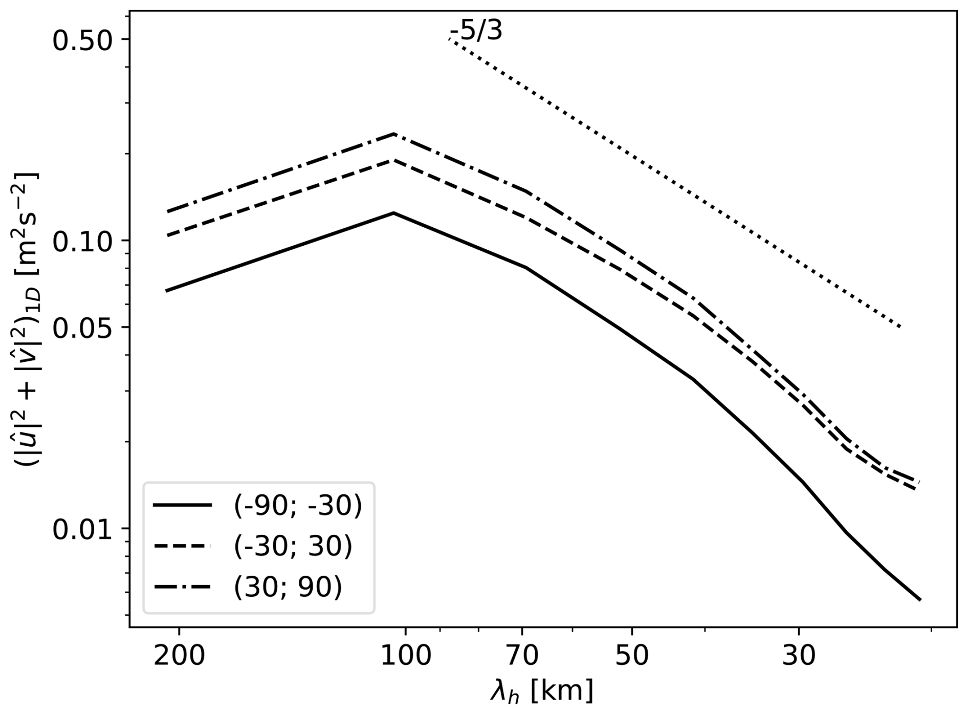
Figure C1 One-dimensional horizontal spectra of kinetic energy density, averaged over the first day of the data for three regions defined by the latitudes 30° N and 30° S. The slopes of the spectra are close to the expected slope −5/3, visualised by the dotted line.

After the projection onto GW modes, the spectra can be described by both the intrinsic frequency and the vertical wavenumber of GWs. We can thus compare the spectra of total energy with the generalised Desaubies spectrum (Fritts and VanZandt, 1993)

$$\begin{array}{}\text{(C1)}& E_{\mathrm{tot}}(m,\widehat{\mathit{\omega }},\mathit{\phi })=B{\left({\displaystyle \frac{m}{m_{\ast }}}\right)}^s{\displaystyle \frac{N^{\mathrm{2}}{\widehat{\mathit{\omega }}}^{-r}}{\mathrm{1}-{\left(\frac{m}{m_{\ast }}\right)}^{s+t}}},\end{array}$$

where φ is the azimuthal direction of propagation, N is the Brunt-Väisälä frequency, B, s, t and r are constants and m_∗ is the characteristic vertical wavenumber. For each direction, this formula represents a power law in $\widehat{\mathit{\omega }}$ and a slightly more complex dependency on m. In Fig. C2, we compare these two dependencies with the spectra obtained from the data for zonally propagating waves ($\mathit{\phi }\in (-\mathrm{45},\mathrm{45})$) for the first day of the simulation, averaged over the globe. To plot the dependency from Eq. (C1), we select r=2, t=3, s=1 and $m_{\ast }=\mathrm{2}\mathit{\pi }/\mathrm{2}$ km (Fritts and Alexander, 2003; Orr et al., 2010; Bölöni et al., 2021). We consider the Brunt-Väisälä frequency to be constant and the constant B is selected so that the magnitude of energy is comparable with the computed spectra.

Qualitatively, the dependency of energy on the intrinsic frequency and vertical wavenumber in Figs. C2a and b is similar to the generalized Desaubies spectrum. In particular, for Fig. C2a, there is a power law for the middle frequencies (period of a few hours), the energy however decreases with the intrinsic frequency faster compared to observations. The observed slope of the spectra is around −2 (Hertzog and Vial, 2001), whereas the slope in Fig. C2a is close to −3. The shape of the spectrum is similar also for other propagation directions.

Similarly, the correspondence of the computed spectra in Fig. C2b with the general form is rather qualitative, with gradual increase of the energy with vertical wavenumber up to a characteristic wavenumber and subsequent decrease of the energy. Although the characteristic vertical wavenumber was selected to correspond to the vertical wavelegth of 2 km, which is a number derived by Fritts and VanZandt (1993) for the tropopause region, the figure suggests that its value depends on the intrinsic frequency and the transition wavelength can be even ten times larger. The structure of the spectrum is again very similar for other propagation direction. Geographically, the increasing part of the plot becomes less prominent in extratropical regions (not shown).

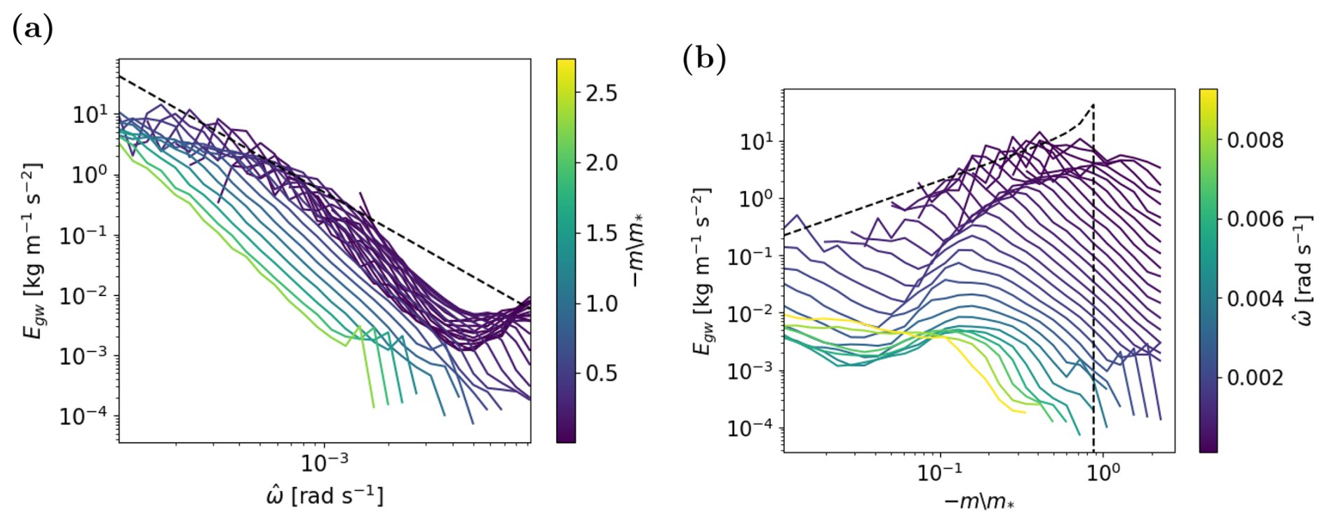
Figure C2 Spectrum of total energy of GWs, evaluated for upward propagating waves with $\mathit{\phi }\in (-\mathrm{45},\mathrm{45})$ for the first day of the simulation, averaged over the globe. (a) Dependence on the intrinsic frequency, (b) dependence on the vertical wavenumber. The figures show a qualitative agreement with the Desaubies spectrum denoted by the dotted line.