Intended and unintended consequences of atmospheric methane oxidation enhancement

Atmospheric oxidation enhancement (AOE) of methane via tropospheric hydroxyl radicals (OH) or chlorine (Cl) radicals is being considered as a method to decrease greenhouse gas concentrations. The chemistry involved is coupled and nonlinear, affecting air quality, other greenhouse gases, and ozone-depleting substances. Here I simulate different OH- and Cl-based AOE methods in a 3D atmospheric chemistry model to estimate their effectiveness and impacts on air quality and climate forcers. I find that larger emissions of iron salt aerosol are required relative to previous work to reduce methane on a global scale by at least a few percent (≥ 565 Tg yr⁻¹), reflecting uncertainty in the reaction mechanism and modeling framework employed. More work is needed to understand the kinetics of chlorine release from iron salt aerosol and the potential for bromine co-release, which decreases effectiveness. Hydrogen peroxide–based approaches can decrease global methane, but feasibility is limited by the large emissions required. Limiting emissions to daytime for hydrogen peroxide–based scenarios has negligible effects. All methods increase surface particulate matter pollution and in some regions lead to exceedances of annual air quality standards. Ozone air pollution decreases under Cl-based methods, but increases in populated areas under OH-based methods. While Cl-based methods can increase ozone-depleting substances, the 1-year timeframe of this study is insufficient to predict impacts on stratospheric ozone. The overall impacts of AOE methods on climate and human health involve not only their effectiveness at decreasing methane, but competing or complementary effects on other greenhouse gases, aerosol, and surface air pollution.

1 Introduction

To achieve aggressive reductions in the greenhouse gas methane needed to reach climate goals, alternate strategies to emissions mitigation are being considered (NASEM, 2024). These include processes to decrease the atmospheric lifetime of methane by enhancing its main sinks (e.g., Abernethy et al., 2023; Gorham et al., 2024; Li et al., 2023b; Ming et al., 2022; Wang et al., 2022), using oxidation by tropospheric OH (currently > 90 %) and tropospheric Cl (currently 1 %–5 %). There are interactions between Cl and OH; namely, increasing Cl decreases OH due to reductions in ozone (e.g., Horowitz et al., 2020; Li et al., 2023b). In addition, Cl and OH can impact aerosol particles, other greenhouse gases, and ozone-depleting substances. Due to these interactions and the highly nonlinear chemistry involved, detailed atmospheric chemical investigations are needed to understand the overall climate and pollution impacts of methods to enhance atmospheric methane oxidation. To have the greatest impact on atmospheric methane, methods appropriate for ambient methane concentrations (≤ 2 parts per million) are needed, but the technology is not yet available (Abernethy et al., 2023; NASEM, 2024; Pennacchio et al., 2024).

While commercial OH generators exist on a smaller scale (e.g., to remove volatile organic carbon pollution; Johnson et al., 2014), it is less well understood how to scale up the artificial production of OH globally (e.g., Ming et al., 2022). Potential technologies could involve the release of hydrogen peroxide, downdraft energy towers, and/or artificial ultraviolet (UV) radiation (Tao et al., 2023; Wang et al., 2022). One specific method to release Cl atom is iron salt aerosol (e.g., Oeste et al., 2017), where the presence of both iron (III) and chloride enhances photolytic Cl atom release. Photolytic Cl atom release from artificial salts has been demonstrated in chamber experiments using salt pans and artificial sea salt aerosols generated from sodium chloride (NaCl) and seawater samples (Wittmer et al., 2015a, b) and in laboratory experiments (Mikkelsen et al., 2024). Recently, this process has been hypothesized to occur in the atmosphere in a study based on observations from Barbados through the mixing of natural iron-containing dust and sea salt aerosols and is thought to be due to the release of chlorine gas (Cl₂) followed by rapid photolysis (van Herpen et al., 2023). Gorham et al. (2024) present the state of the science for moving forward with intentional increase of this mechanism via iron salt aerosol. Meidan et al. (2024) find that the impact of iron varies depending on the region of application. Recent work has investigated the direct release of Cl₂ in a coupled chemistry–climate model and found that at least 90 Tg yr⁻¹ Cl₂ is needed for Cl increases to outweigh decreases in OH with respect to overall methane loss, and at least 1,250 Tg yr⁻¹ Cl₂ is needed to decrease the methane lifetime by 50 % or more (Li et al., 2023b).

Here I simulate in an atmospheric model a variety of methods of atmospheric oxidation enhancement (AOE) of methane via tropospheric OH and tropospheric Cl. I assess their impacts on methane, tropospheric chemistry, other greenhouse gases and ozone-depleting substances, and surface air quality.

2 Methods

I apply the global atmospheric chemical transport model GEOS-Chem (Sect. 2.1) with modifications (Sect. 2.2) to simulate atmospheric oxidation enhancement scenarios and their effects. The overall methodology of the study is outlined in Fig. S1 in the Supplement.

2.1 GEOS-Chem Model

Here I apply the 3D atmospheric chemical transport model GEOS-Chem version 13.2.1. (https://doi.org/10.5281/zenodo.5500717, The International GEOS-Chem User Community, 2021). As it is a chemical transport model, meteorological and climatic processes are not simulated directly. Instead, the model is driven by assimilated offline meteorological fields of the Modern-Era Retrospective Analysis for Research and Applications (Gelaro et al., 2017) from the National Aeronautics and Space Administration/Global Modeling and Assimilation Office. Simulations are performed at 4° latitude × 5° longitude horizontal resolution, with 72 vertical layers from the surface to the mesosphere (up to 80 km) and with active chemistry through the stratosphere (up to 50 km). Simulations are performed for the arbitrary year 2019 following 1 year of initialization (year 2018). The below describes what will be referred to as the “Standard” simulation in the Results (Sect. 3).

Detailed coupled tropospheric halogen (chlorine, bromine, iodine) chemistry follows Wang et al. (2021) and includes sea salt debromination, acid displacement, and improvements to heterogeneous chemistry on polar stratospheric clouds (Eastham et al., 2014). Online stratospheric chemistry includes heterogeneous ozone depletion chemistry. Aerosols are assumed to be fully internally mixed. Carbonaceous aerosol includes black carbon (Wang et al., 2014) and organic aerosol following the “simple” secondary organic aerosol (SOA) scheme (fixed-yield, direct, and irreversible formation) (Pai et al., 2020). Anthropogenic emissions follow the Community Emissions Data System (CEDS) v2 inventory originally developed for the Coupled Model Intercomparison Project Phase 6 (CMIP6) (https://data.pnnl.gov/dataset/CEDS-4-21-21, last access: 7 October 2024), including particulate iron (pFe) emitted as a constant fraction of sulfur dioxide (SO₂). The speciation and solubility of iron in GEOS-Chem is discussed in Sect. 2.2.2. Sea salt aerosol emissions over the open ocean are wind- and sea surface temperature–dependent following Jaeglé et al. (2011), and in polar regions include blowing snow (Huang and Jaeglé, 2017). Dust emissions include natural (Fairlie et al., 2007) and anthropogenic dust from the anthropogenic fugitive, combustion, and industrial dust inventory (Philip et al., 2017). Biogenic volatile organic compound emissions are from MEGAN v2.1 (Guenther et al., 2012). All meteorologically dependent emissions are calculated offline at the native resolution of the MERRA-2 meteorology (0.5° × 0.625°) (Weng et al., 2020) and appropriately scaled such that the total emissions are independent of model resolution (Lin et al., 2021). Wet deposition follows Amos et al. (2012) for gases and Liu et al. (2001) for aerosols, with snow and mixed precipitation scavenging from Wang et al. (2014). Dry deposition is a resistance-in-series approach (Wang et al., 1998) with aerosol dry deposition described in Zhang et al. (2001). Ozone deposition to the ocean via reaction with sea surface iodide follows Pound et al. (2020). Planetary boundary layer mixing follows a non-local scheme (as opposed to assuming full mixing) as implemented by Lin and McElroy (2010). The first 2 km contain 14 vertical levels, with gridbox heights increasing from 120 m at the surface to 250 m by 2 km.

Methane concentrations at the surface in GEOS-Chem are a fixed boundary condition based on monthly mean National Oceanic and Atmospheric Administration flask observations, after which methane advects and participates in chemistry (Murray, 2016). Hence, I use the methane feedback factor, which accounts for the feedback of methane on its own loss rate to estimate changes in steady-state methane concentrations. Impacts on steady-state methane concentrations estimated using fixed boundary conditions along with the methane feedback factor are within 10 % of impacts predicted from long (> 40 years) simulations reaching equilibrium with fully responsive surface methane fluxes, while significantly reducing the computational cost (Khodayari et al., 2015). Fixed boundary conditions combined with the feedback factor also have been found to have a negligible impact on estimates of the global warming potential of hydrogen accounting for indirect methane feedbacks (Warwick et al., 2023). Here, I first calculate the methane lifetime following the same methods as in Horowitz et al. (2020) from Holmes et al. (2013) and Holmes (2018). Briefly, the partial lifetimes of methane against tropospheric OH and Cl are calculated from the integrated 3D reaction rates. The total methane lifetime includes these two losses, stratospheric loss (assumed 120 years), and uptake to soil (assumed 150 years). Then, the change in steady-state methane concentration is estimated using the feedback factor f following Holmes (2018):

$$\begin{array}{}\text{(1)}& \mathrm{\Delta }\left[{\mathrm{CH}}_{\mathrm{4}}\right]=\left({\left({\displaystyle \frac{{\mathit{\tau }}_{\exp }}{{\mathit{\tau }}_{\mathrm{0}}}}\right)}^f-\mathrm{1}\right){\left[{\mathrm{CH}}_{\mathrm{4}}\right]}_{\mathrm{0}}\end{array}$$

where τ₀ and τ_exp are the lifetimes of methane in the standard and atmospheric oxidation enhancement experiments, respectively; f = 1.34 ± 0.06 is the GEOS-Chem methane feedback factor on its loss rate (Holmes et al., 2013); and [CH₄]₀=1866.58 parts per billion (ppb) is the global annual mean surface methane concentration in year 2019 (https://gml.noaa.gov/ccgg/trends_ch4/, last access: 7 October 2024).

2.2 Model Experiments for Atmospheric Oxidation Enhancement

A summary of simulations is presented in Fig. S2. Scenarios are grouped between the dominant intended effect on increasing methane oxidation, either through reaction with OH (OH-based; Sect. 2.2.1) or Cl (Cl-based; Sect. 2.2.2). Under these umbrellas are experiments with different compounds emitted (OH or hydrogen peroxide for OH-based, and Cl₂ or particulate iron and/or chloride for Cl-based). All emissions are constant in time except for daytime-only tests (for simplicity, double the 24 h emissions rate released between 06:00 and 18:00 LT) for several of the hydrogen peroxide emissions scenarios, as marked in Table 1 and Fig. S2.

Table 1 Details of focus scenarios in the current study.

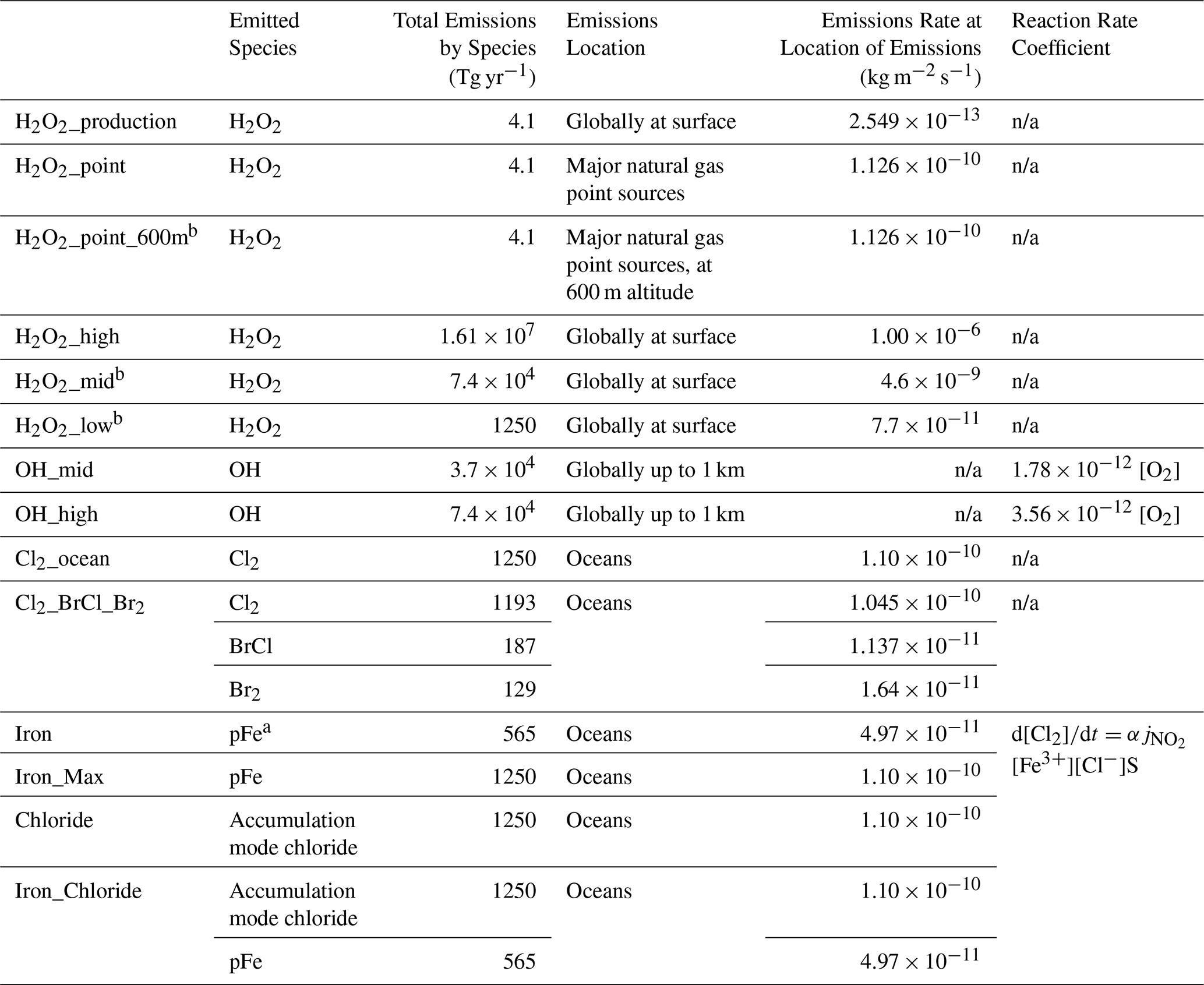
^a pFe is particulate iron. ^b Scenario was also tested with 2 × emissions during daytime only (06:00–18:00 LT).

2.2.1 Hydroxyl Radical

Hydrogen peroxide emission

Hydrogen peroxide photolysis produces two OH radicals, and the emission of hydrogen peroxide has been proposed as a possible method to enhance atmospheric methane oxidation via OH (Wang et al., 2022). For example, there is a patent to deploy hydrogen peroxide towers for this purpose (Bell, 2023). The concurrent production of hydrogen peroxide and release of OH via Fenton-like catalytic processes has also been suggested as a potential technology (Wang et al., 2022).

In this study, I tested four scenarios to investigate the impact if the current global demand of 4.1 Tg yr⁻¹ H₂O₂ (Research and Markets, 2023) was released additionally (see Fig. S2): globally at the surface, only at major point sources of oil and gas emissions determined from the CEDS anthropogenic emissions inventory (0.2 % of Earth's area at the 4° × 5° model resolution) at the surface, 600 m (stack height proposed by the Bell, 2023, patent), and 600 m emitted only during daytime to maximize photolysis. Three global hydrogen peroxide emissions scenarios to span a range of impacts on methane and feasibility (H₂O₂_high, H₂O₂_mid, and H₂O₂_low; see Table 1). H₂O₂_low emits the same mass as the Cl₂ experiment (1250 Tg yr⁻¹; see Sect. 2.2.2) for comparison purposes. Short-term tests were performed with increasing H₂O₂ emissions to estimate the quantity needed such that methane would decline by at least 50 % (leading to H₂O₂_high). All scenarios were emitted at the surface (0 to 12.3 m altitude in GEOS-Chem). I also tested H₂O₂_mid and H₂O₂_low with double the 24 h emissions rate only released during 06:00–18:00 LT.

OH chemical production

Not all hydrogen peroxide is immediately photolyzed to produce OH and may undergo alternate reactions. Estimates include the previously described GEOS-Chem study which found approximately 30 %–60 % of H₂O₂ on average is photolyzed, but this is highly spatially variable (Mayhew and Haskins, 2025), and a conservative theoretical estimate of 10 % based on all potential chemical and physical pathways (Pennacchio et al., 2024). Thus, to examine the direct effects of OH release in the absence of other chemical changes, I introduced a dummy reaction in GEOS-Chem to produce OH from O₂, a species with fixed concentrations in GEOS-Chem (0.2095 mol mol⁻¹), from the surface up to 1 km altitude globally (see Table 1). OH cannot be advected in GEOS-Chem due to its short lifetime and thus it cannot be emitted directly. I tested two rates, OH_mid and OH_high; OH_high's rate of OH emission is two times higher (see Table 1) to result in similar changes to OH as the hydrogen peroxide simulations (since H₂O₂ photolyzes to produce 2OH). In reality, OH could be released directly through methods incorporating artificial UV radiation (e.g., Ming et al., 2022) or downdraft energy towers that generate electricity from seawater and sunlight and produce additional OH from ozone due to the water vapor introduced in dry regions (Tao et al., 2023; Wang et al., 2022); these would likely be point sources that are not feasible in the current modeling framework. Given this and the fixed methane boundary conditions, the direct OH results will only be discussed in reference to how air quality impacts change when OH versus hydrogen peroxide is emitted at comparable impacts on methane.

2.2.2 Chlorine

Direct Cl₂ emission

In the Cl₂ simulation, Cl₂ is directly emitted across the global oceans at the surface, a total of 1250 Tg yr⁻¹, which is the midrange scenario for methane removal in Li et al. (2023b) (resulting in 45 % reduction in the methane burden in their study). This is approximately 20 times higher than the current total tropospheric source of gas-phase inorganic chlorine in GEOS-Chem (54 Tg yr⁻¹; Wang et al., 2021) or the current manufacture of Cl₂ (58 Tg yr⁻¹; World Chlorine Council, 2024). Emissions of Cl₂ at the surface are more likely to be economically and technologically feasible and will limit the impact of additional chlorine on stratospheric ozone (Li et al., 2023b). Cl₂ will then photolyze to produce two Cl atoms, of which approximately 20 % will react with ozone instead of methane over the oceans (Li et al., 2023b). Table S2 compares the modeling setup of the current study and Li et al. (2023b), including differences in resolution, year, and halogen chemistry.

Bromine contamination

It is not possible to remove 100 % of bromide from pure chloride salts (for example, Sigma-Aldrich S9888 ≥ 99.0 % NaCl specifications include up to 0.01 % Br⁻; https://www.sigmaaldrich.com/, last access: 31 January 2026). This could lead to reactive bromine release that would decrease OH in the atmosphere through the destruction of ozone, the primary HO_x (HO_x = OH + HO₂) source (e.g., Horowitz et al., 2020), while unlike Cl it does not also oxidize methane. Here I create a model experiment (Cl₂_BrCl_Br₂) including direct emission of the bromine species Br₂ and BrCl. Wittmer et al. (2015b) measured the Br versus Cl production rate from artificial sea salt created from a variety of iron-containing artificial seawater or NaCl stock solutions, with the ratio of Br/Cl produced by mass ranging from 0 to a factor of 2.5. Br atom was below the detection limit for the NaCl-based solutions (Wittmer et al., 2015b), which may better resemble artificially engineered iron salt aerosol. However, previous work with salt pans found that even when Br atom concentrations were below the detection limit, bromide impurities in “pure” NaCl (≤ 0.01 % Br⁻) could lead to Cl atom release due to BrCl formation and photolysis, which would also release Br atoms in equal quantities (Wittmer et al., 2015a). Here I assume that of the total desired chlorine release (1250 Tg yr⁻¹ as in the Cl₂-ocean simulation), 20 % of that by mass of bromine is released in equal parts Br₂ and BrCl (resulting in 1193 Tg yr⁻¹ Cl₂, 187 Tg yr⁻¹ Br₂, and 129 Tg yr⁻¹ BrCl). This scenario represents a bounding case if artificial sea salt containing bromine impurities were to be continuously emitted as part of an AOE method. In prior work, increasing the flux of natural sea salt aerosol in GEOS-Chem led to relative increases in tropospheric-wide reactive bromine that were comparable to that of reactive chlorine (Horowitz et al., 2020). More laboratory studies are needed to understand the potential bromine release from engineered iron salt aerosol.

Implementation of Chen et al. (2024) iron salt aerosol mechanism

Here I implement a parameterization of photolytic Cl₂ release from iron-enriched salt aerosol developed by Chen et al. (2024) on top of the Standard simulation described in Sect. 2.1. The below describes what will be referred to as the “Standard + Chen” simulation in the Results (Sect. 3). The production rate of Cl₂ ($\mathrm{d}\left[{\mathrm{Cl}}_{\mathrm{2}}\right]/\mathrm{d}t$: molec. cm⁻³ s⁻¹) is a function of the nitrogen dioxide (NO₂) photolysis frequency ($j_{{\mathrm{NO}}_{\mathrm{2}}}$: s⁻¹), accumulation mode aerosol iron (III) concentration ([Fe³⁺]: mol L⁻¹ water, or M), accumulation mode aerosol chloride concentration ([Cl⁻]: M), and aerosol surface area concentration (S: µm² cm⁻³), and is scaled by the factor α (= 1.4 × 10⁵ molec. µm⁻² M⁻²) based on experimental results from Wittmer et al. (2015b) accounting for the volume of the chamber:

$$\begin{array}{}\text{(2)}& \mathrm{d}\left[{\mathrm{Cl}}_{\mathrm{2}}\right]/\mathrm{d}t=\mathit{\alpha }{j}_{{\mathrm{NO}}_{\mathrm{2}}}\left[{\mathrm{Fe}}^{\mathrm{3}+}\right]\left[{\mathrm{Cl}}^{-}\right]S\end{array}$$

This reaction (Cl⁻ → 0.5 Cl₂) occurs on chloride in accumulation mode sea salt aerosol, which in GEOS-Chem is defined as ≤0.5 µm in diameter. Additional details on the parameterization calculations including α and the chamber volume correction are presented in Sect. S1 and Table S1 in the Supplement.

Spatiotemporally varying photolysis frequencies (including $j_{{\mathrm{NO}}_{\mathrm{2}}}$) are calculated online in GEOS-Chem using the Fast-JX scheme (Neu et al., 2007) as implemented by Mao et al. (2010) and account for cloud optical depth. In the standard GEOS-Chem model, Fe(III) concentrations are estimated from natural dust up to 1 µm and anthropogenic particulate Fe (pFe) for the Fe(III)-catalyzed SO₂ oxidation chemistry. This assumes that total Fe content from dust is 3.5 % of total mass (Taylor and McLennan, 1985; consistent with Trapp et al., 2010), dust iron solubility is 1 % (Alexander et al., 2009) while anthropogenic particulate Fe is more soluble at 10 % (Shao et al., 2019), and Fe(III) is 10 % of total dissolved iron in the daytime (Moffet et al., 2012) and 90 % at night. These assumptions are not sufficient to match observations in polluted urban environments in China (Chen et al., 2024). Model evaluation against observations suggests four times higher solubility for both dust and anthropogenic Fe (4 % and 40 %, respectively) and 67 % of total dissolved iron as Fe(III) (Chen et al., 2024). Observed Fe solubility in aerosols over the oceans is highly variable (0.19 % to 47.8 %) and is influenced by the initial source of the iron (e.g., dust vs. combustion), other chemical components in the aerosol, pH, and relative humidity (Shi et al., 2022). For the iron salt aerosol simulations, I use the Chen et al. (2024) representation of solubility and Fe(III) speciation as a maximum rate of Cl₂ production through this particular parameterization. For consistency with the version of the Chen et al. (2024) mechanism that was evaluated against observations (see Sect. 3.2), I also include this process on fine-mode aerosols only; the chamber experiment on which the mechanism is based used fine mode aerosol (Wittmer et al., 2015b) and the lifetime of smaller particles is longer relative to coarse particles such that iron and chloride have time to mix within the aerosols before being deposited (Moffet et al., 2012; Zhu et al., 2022). The dependence on aerosol surface area concentration, and the impacts of pH and potential suppression of the rate by aerosol sulfate and organics (which are not considered in this mechanism) warrant future study. van Herpen et al. (2023) also parameterized the production of Cl₂ from natural mineral dust–sea spray aerosols. Major differences between Chen et al. (2024) and van Herpen et al. (2023) include the size of the particles on which this process occurs, the percentage of photoactive iron, and that the Chen et al. (2024) study is based primarily on the Wittmer et al. (2015b) chamber experiments while van Herpen et al. (2023) follow the Fe(II)–Fe(III) cycling kinetics from Zhu et al. (1993). Differences in the model frameworks are summarized in Table S3.

Iron salt aerosol emissions experiments

First I perform GEOS-Chem simulations with the additional reaction of iron-mediated Cl₂ release from chloride aerosol from Chen et al. (2024) (Standard + Chen simulation; Sect. 2.2.2, “Implementation of Chen et al. (2024) iron salt aerosol mechanism”) in the absence of any additional emissions to act as a reference point for the iron salt aerosol emissions-based atmospheric oxidation enhancement experiments. Then, within the Standard + Chen simulation to release additional Cl₂ from iron salt aerosol, accumulation mode aerosol chloride (Cl⁻) and particulate iron (pFe) are released over the oceans at the surface in four scenarios to assess the driving factors and compare against the direct Cl₂ scenario. Accumulation mode aerosol Cl⁻ and pFe are existing species within GEOS-Chem, where Cl⁻ is sea salt chloride with the physical properties of sea salt aerosol and the molecular weight of chlorine, and pFe represents anthropogenic particulate iron (see also Sect. 2.1 and 2.2.2, “Implementation of Chen et al. (2024) iron salt aerosol mechanism”). The highest iron addition tested in Wittmer et al. (2015b) was 13 mol Cl⁻ mol⁻¹ Fe³⁺. Given the assumed solubility of anthropogenic pFe of 40 % and Fe(III) speciation fraction of 67 % in my GEOS-Chem simulations, a ratio of 3.484 mol Cl⁻ mol⁻¹ pFe emitted would lead to Fe(III) ratios at most comparable to the highest iron addition experiments in Wittmer et al. (2015b). For accumulation mode aerosol chloride emissions of 1250 Tg (the same mass of total chlorine emissions as the Cl₂ experiment), this is 565 Tg yr⁻¹ pFe. The photoactive fraction of the emitted particulate iron for AOE model experiments is the same as other anthropogenic pFe, and is 26.8 % (see Table S3) by accounting for both the solubility and Fe(III) speciation fractions. The experiments here include particulate iron emissions alone (Iron), aerosol chloride emissions alone (Chloride), a combination of both particulate iron and chloride (Iron_Chloride), and particulate iron alone emitted at 1250 Tg yr⁻¹ (Iron_Max) as a test case (see Table 1 for details). Iron_Max does not lead to significantly more methane loss than the Iron scenario; hence, it will only be discussed in the context of methane and not with respect to tropospheric chemistry and air quality.

3 Results

Several hydrogen peroxide experiments produced negligible results. I will discuss these briefly here and for the remainder of the paper focus on experiments with non-negligible changes in methane. All 4.1 Tg yr⁻¹ H₂O₂ scenarios (H₂O₂_production, H₂O₂_point, and H₂O₂_point_600m; see Table 1) produced negligible effects on the methane lifetime. The change to 600 m stack height as well as from 24 h to daytime-only emissions did slightly increase the impact on methane (by ≪ 1 %) but still resulted in < 0.5 ppb (≤ 0.03 %) decrease in methane. As the spatial resolution is low (4° × 5° or 400–500 km at midlatitudes), this current model study may not address fully whether this method is viable for individual, large point sources of methane. Given the negligible results found here, these scenarios were not investigated further in this study. Another study using the GEOS-Chem model investigated daytime-only 600 m H₂O₂ towers in more detail over North America at a higher spatial resolution (0.5° × 0.625° or ∼ 50 km), and found that even widespread towers at emissions rates 10 × higher than what is currently proposed would lead to negligible impact on global methane (Mayhew and Haskins, 2025). This is in part because the fraction of H₂O₂ converted to OH is ∼ 30 %–60 % but is driven by the small fraction of the produced OH that reacts with methane (23 % at the most and frequently much less) (Mayhew and Haskins, 2025).

3.1 Impacts on Major Tropospheric Oxidants and Reactive Halogens

Table 2 presents the tropospheric burdens of major oxidants, reactive halogen families, and carbon monoxide (CO) for the standard GEOS-Chem simulation and the standard simulation plus the Chen et al. (2024) parameterization, followed by relative percent changes in these burdens for the atmospheric oxidation enhancement model experiments described in Table 1.

Table 2 Simulated global annual mean tropospheric burdens of selected species and chemical families and their percent change due to atmospheric oxidation enhancement.

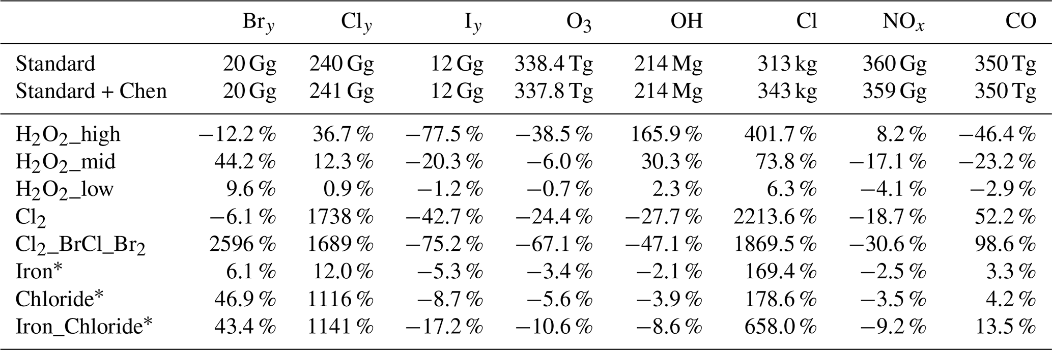
Note: Percent change in annual mean tropospheric burdens for model experiments (described in Table 1) are relative to the standard version (^∗ = relative to standard + Chen et al., 2024). Br_y, Cl_y, and I_y follow definitions in Wang et al. (2021); NO_x = NO + NO₂. See also Sect. 2.1.

Previous work on an intermodel comparison of atmospheric chemistry and climate models from the Atmospheric Chemistry and Climate Model Intercomparison Project found that changes in global mean OH between models and within a given model are more a function of the relative loss of reactive nitrogen versus reactive carbon than the emissions of reactive nitrogen versus carbon, as it matters how much of the loss of these species is due to OH versus other processes (Murray et al., 2021). The loss of reactive carbon is a function of a given model's chemical mechanism and structure (Murray et al., 2021). The GEOS-Chem model version used in this study (13.2.1) is several generations ahead of that used in Murray et al. (2021) (version 9-01-03), with a number of changes in reactive nitrogen chemistry including aerosol uptake and recycling of isoprene nitrates (e.g., Fisher et al., 2016, 2018; Holmes et al., 2019; McDuffie et al., 2018) that have been shown to impact the tropospheric OH burden by up to 12 %. The representation of nitrogen oxides (NO_x) loss thus can lead to uncertainty in the simulated OH burden, but it is not clear if this would be a consistent bias across all model experiments in the current study and thus negligible when considering relative changes.

As expected, the hydrogen peroxide experiments all increase tropospheric OH due to photolysis of the additional hydrogen peroxide. OH does not increase proportionally to the increase in hydrogen peroxide emissions across experiments and indicates a reduction in the effectiveness of additional emissions at higher levels of hydrogen peroxide. A > 200-fold increase in hydrogen peroxide emissions from H₂O₂_mid to H₂O₂_high leads to a 5.5-fold increase in the change of OH; a 60-fold increase in hydrogen peroxide emissions from H₂O₂_low to H₂O₂_mid leads to a 13-fold increase in the change of OH (see Table 2). The increases in OH drive reductions in tropospheric CO seen in these experiments, as OH is the main oxidant of CO. The reductions in CO are nearly proportional to the OH increases in the H₂O₂_low and H₂O₂_mid scenarios; however, in the extreme H₂O₂_high scenario, the CO decrease is much lower than expected from the OH increase (see Table 2). This is likely due to the much larger increase in Cl atom in the H₂O₂_high experiment, leading to additional production of CO from Cl reactions with formaldehyde and organochlorines (see Table S4). In all of the hydrogen peroxide experiments, Cl atom increases. Increased HO_x (= OH + HO₂, which cycle rapidly between each other) leads to increased release of chlorine from sea salt aerosol and organohalogens (see Table S4 and Wang et al., 2021), increasing the total Cl_y burden. Within each experiment, the longer-lived reservoir species hydrogen chloride (HCl) contributes the largest mass to the total Cl_y burden. However, relative to the standard simulation the partitioning of gas-phase Cl_y in the H₂O₂ experiments shifts away from HCl toward chlorine hydroxide (HOCl), Cl₂, and Cl, such that the relative increase in Cl atom is greater than the relative increase in total Cl_y for each experiment. This is due to the complex interplay of cross-reactions between fast-cycling HO_x and chlorine radicals as well as across their longer-lived reservoir species. For example, in addition to the reactions in Table S4 which are sources of gas-phase Cl_y rather than cycling between species, OH can react with HCl to produce Cl atom.

Cl-based experiments decrease tropospheric OH due to the destruction of ozone by the additional Cl, as ozone provides the main source of tropospheric OH. Tropospheric CO increases in the chlorine-based experiments, partially due to the decrease in OH as well as the additional production of CO from reactions of formaldehyde and organochlorines with Cl atom. The Cl₂, Chloride, and Iron_Chloride experiments have the same amount of total chlorine emissions (see Table 1) but vastly different effectiveness at increasing the Cl atom concentration due to the emitted species (gas-phase Cl₂ or particulate chloride) having different reactivities and reactions. The Chloride and Iron_Chloride experiments, where particulate accumulation mode chloride was emitted, have 64 % to 66 % as much of an increase in total gas-phase Cl_y burden relative to the Cl₂ experiment where gas-phase Cl₂ was emitted (see Table 2). However, only 8 % (Chloride only) to 30 % (Iron_Chloride) of the increase in Cl atom seen in the Cl₂ experiment is realized. This is because the vast majority of the increase in Cl_y burden in these experiments is due to HCl, shifting Cl_y away from more reactive species. As in the hydrogen peroxide experiments, HCl still remains the dominant component of Cl_y. The release of Cl₂ is iron-limited, as the addition of particulate iron emissions with the same amount of chloride (from Chloride to Iron_Chloride) leads to a nine-fold increase in Cl₂ and a three-fold increase in Cl (see Table S5).

In the Cl₂ and Cl₂_BrCl_Br₂ experiments, Cl_y partitioning is shifted away from HCl to Cl₂ and Cl. Thus, the relative increase in Cl atom is even greater than the relative increase in total tropospheric Cl_y (see Table 2). In Li et al. (2023b), 1250 Tg yr⁻¹ Cl₂ led to a 30-fold increase in the tropospheric Cl burden; these emissions in our shorter-term modeling study led to a 23-fold increase in the Cl₂-only case and a 20-fold increase in the Cl₂_BrCl_Br₂ case (where 1250 Tg yr⁻¹ of total chlorine was split between 1193 Tg yr⁻¹ as Cl₂ and the remainder as BrCl). In GEOS-Chem, the only fate of BrCl is photolysis to produce Cl atom. Hence, the smaller impact of the Cl₂_BrCl_Br₂ scenario on total tropospheric Cl atom is due to the increases in Br_y in this experiment (see Table 2) and the coupled chemistry of Br_y species with Cl_y cycling.

All experiments decrease the tropospheric ozone burden (see Table 2), with implications for ozone radiative forcing. All experiments have increased Cl atom concentrations, which can destroy ozone. H₂O₂_low, H₂O₂_mid, and all chlorine experiments except Cl₂ also have increased Br_y burdens, which can lead to additional ozone loss via reactive bromine. Increases in OH in the hydrogen peroxide experiments could lead to increased sources of Br_y from sea salt and organohalogens (see Table S4 and Wang et al., 2021). In the H₂O₂_low, H₂O₂_mid, and chlorine experiments, part of the change in ozone is also due to reductions in NO_x that lead to reduced ozone production. This is consistent with previous work which found more active halogen chemistry leads to reductions in NO_x (e.g., due to hydrolysis of halogen nitrates) (e.g., Wang et al., 2019, 2021; Sherwen et al., 2016b; Horowitz et al., 2020). The increases in Br_y and decreases in NO_x, which became larger as hydrogen peroxide emissions increase from H₂O₂_low to H₂O₂_mid, flip sign once hydrogen peroxide emissions become particularly extreme in the H₂O₂_high scenario. Thus in the H₂O₂_high case, the ozone loss is likely dominated by the large increase in Cl atom (see Table 2).

As seen in Horowitz et al. (2020), the decreases in ozone drive decreases in tropospheric I_y in all experiments, as ozone reactions with sea surface iodide are the dominant source of tropospheric I_y (Wang et al., 2021). The greatest impacts on ozone are in the Cl₂_BrCl_ Br₂ experiment, which included bromine release to represent bromide contamination (see Table 1). The 20 % additional mass released as bromine (Br₂ and BrCl, which both photolyze to release Br atom) led to a much larger than 20 % additional reduction in ozone over the Cl₂-only experiment (factor of 2.75 higher) and hence OH (factor of 1.70 higher) (see Table 2). While 20 % is likely an overestimate of the bromide content of engineered aerosol, it is well within the range reported from natural seawater salt experiments catalyzed by iron (Wittmer et al., 2015b) and suggests that even a small perturbation in bromine could have a much larger impact on OH.

The OH_mid and OH_high scenarios lead to 51 % to 94 % increases in OH, respectively (see Table S6). Despite a much larger increase in OH in OH_high than in OH_mid, the decrease in CO is only 5 % larger. The OH experiments' results for CO are less reliable than the H₂O₂ experiments as the OH increase is limited to the lower 1 km where it is released. (OH is not transported in the model; hydrogen peroxide is.) In this region, methane levels remain high due to the surface boundary condition and long lifetime against reaction with OH; as CO does not have a fixed surface boundary condition, here it is reacted away by the additional OH, and its loss rate slows down due to its shorter lifetime.

3.2 Impacts on Methane

Figure 1 (top panel) summarizes the impacts on the overall methane lifetime, the impacts on the methane lifetime with respect to tropospheric OH, and the percent of Cl atom contributing to total chemical loss in the troposphere for each of the experiments in Table 1 and the standard model. Figure 1 (bottom panel) shows the resulting relative change in steady-state methane concentrations estimated with the methods described in Sect. 2.1.

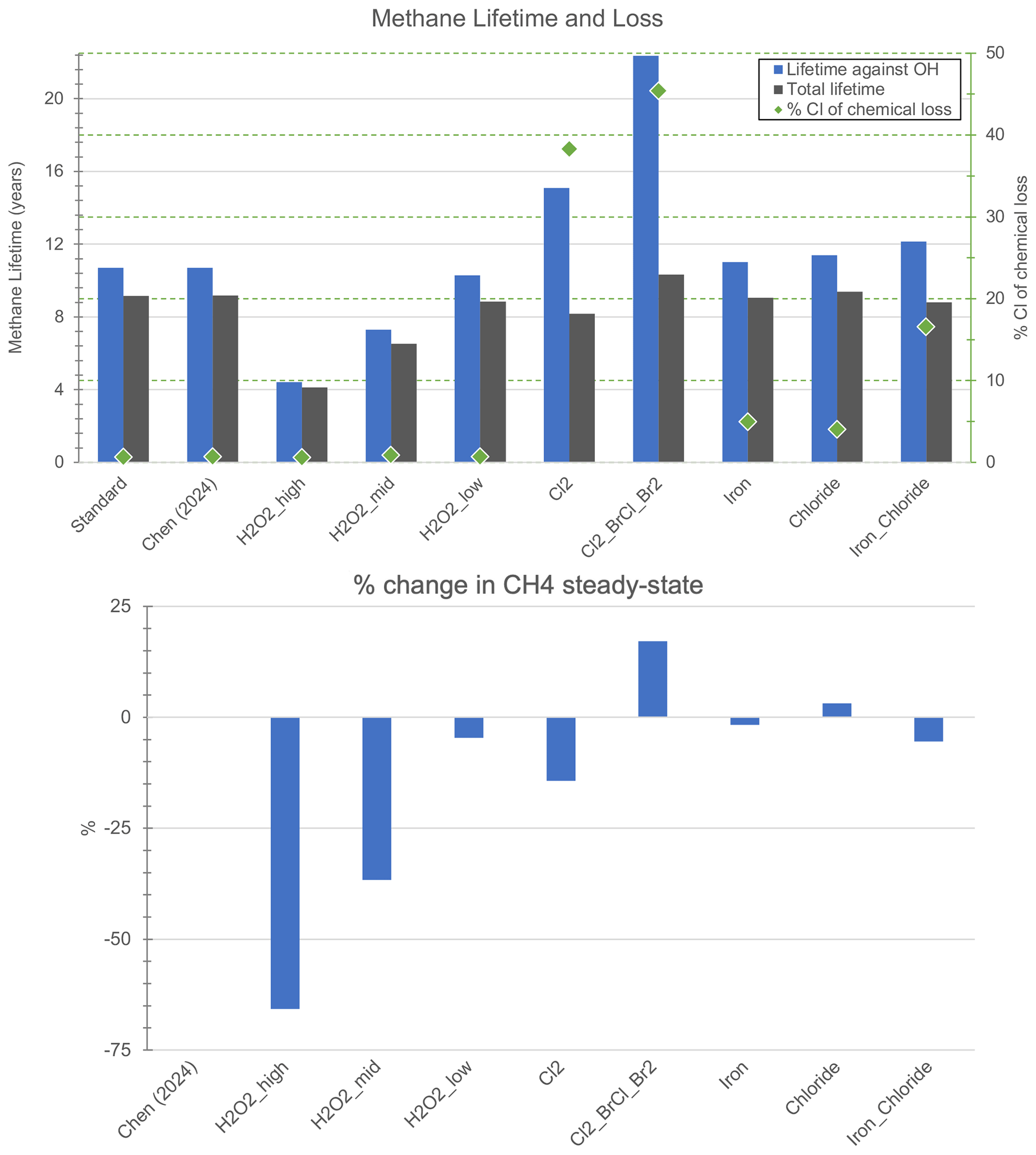
Figure 1 Top panel: total methane lifetime (gray bars) and methane lifetime against oxidation by OH (blue bars), overlaid by the percent of chemical loss contributed by Cl atom (green diamonds, right-hand y-axis). Bottom panel: estimated relative percent change in steady-state methane concentration.

Studies suggest that the present role of chlorine in tropospheric methane oxidation is 0.23 %–5 % based on constraints from isotopic observations (Allan et al., 2007; Gromov et al., 2018; Platt et al., 2004) and atmospheric modeling studies focused on chlorine chemistry (e.g., Hossaini et al., 2016; Wang et al., 2019, 2021). The standard version of GEOS-Chem used here is consistent with these constraints at 0.7 %, which gives confidence to the simulation of atomic chlorine and its reaction with methane.

Although the H₂O₂_high experiment had more than 5x greater increase in tropospheric OH than that of H₂O₂_mid (see Table 2), the methane lifetime against OH decreases by less than a factor of 2 (Fig. 1). The efficacy of H₂O₂ with respect to oxidizing methane via tropospheric OH and decreasing steady-state methane concentrations decreases with increasing emissions (see Fig. S3). There is a larger difference between the scenarios for the change in steady-state methane, which also accounts for changes in the lifetime against tropospheric Cl. While all H₂O₂ experiments also lead to increased Cl atom (see Table 2), H₂O₂_low is most efficient at also decreasing the methane lifetime against oxidation by tropospheric Cl for its smaller level of emissions (Fig. S3). Significant methane reductions for the hydrogen peroxide scenarios (> 5 %) require more than 1,250 Tg yr⁻¹ emissions (H₂O₂_low). In the 4.1 Tg yr⁻¹ point source tests, impacts increased slightly when the hydrogen peroxide was emitted at 600 m vs. at the surface. It is thus possible that the impacts on methane by these global scenarios could be larger if emitted at 600 m, potentially due to a longer lifetime for H₂O₂ allowing for greater photolysis; this would require further investigation. I also tested H₂O₂_mid and H₂O₂_low with double the 24 h emissions rate only released during 06:00–18:00 LT. Daytime-only emissions did increase the impact on methane, with a larger relative effect for the smaller hydrogen peroxide emissions, but the absolute values of methane lifetime and steady-state methane concentrations are within ±1 % for the corresponding daytime-only and 24 h emissions scenarios. Thus, I will focus on results from the 24 h emissions for the remainder of the paper.

For the same annual emissions of Cl₂ (1250 Tg yr⁻¹) as in Li et al. (2023b), I find slightly smaller decreases in the methane lifetime (here −11 % vs. −50 %) and methane concentrations (here −14 % at steady-state vs. −45 % in year 2050) despite vastly different modeling frameworks (Table S2). Li et al. (2023b) finds a larger increase in the tropospheric burden of Cl atom, as described in the previous section (factor of 30 vs. factor of 23), and a larger percent of methane chemical loss due to tropospheric chlorine (60 % vs. 38 %). The baseline present-day tropospheric Cl burden in Li et al. (2023b) was also larger (0.7 Mg vs. 0.313 Mg in this study). In addition, differences in our results may be due to differences in the vertical distribution of Cl as well as the meteorology between the two models, as the Cl + CH₄ reaction is temperature-dependent (see Table S4) and the impacts of local changes in the reaction rate on the global methane lifetime are weighted by air density. While a quantitative comparison of the vertical distribution of Cl concentrations between the two models is not able to be conducted here, I hypothesize that model differences may influence this distribution. The vertical distribution of Cl in the two models is not only impacted by the halogen chemical mechanism (see Table S2); in GEOS-Chem, an improved representation of entrainment-limited uptake in clouds and ice cloud particle properties for cloud heterogeneous chemistry leads to significant increases in reactive chlorine, particularly in the upper troposphere where reaction rates are decreased due to low temperatures (Table S6), due to changes in HCl-ClO_x (chlorine oxides) cycling (Holmes et al., 2019). Other differences that could impact the results are the increase in methane emissions in Li et al. (2023b) following the representative concentration pathway 8.5 scenario, and the shorter simulation period in our study (see Table S2). Bromine contamination of 20 % more than reverses the gains seen in the Cl₂ case, as the Cl₂_BrCl_ Br₂ case has an increase in steady-state methane concentrations of 17.2 % (see Fig. 1).

Figures 2 and S4 show the change in annual mean Cl₂ and Cl atom concentrations at the surface and zonally averaged through 20 km, respectively, from adding the Chen et al. (2024) mechanism for Cl₂ production from aerosol iron photochemistry. The absolute increase in surface [Cl] (Fig. 2) is largest over the North Atlantic ocean, with the largest relative increases over China reaching a factor of 3 (204 %). In Chen et al. (2024), simulations were performed for 9–31 December 2017 over North China at 16 times higher spatial resolution (0.25° latitude × 0.3125° longitude) than this study (4° × 5°). They also added high-resolution anthropogenic fine-mode aerosol Cl⁻ emissions in China from Fu et al. (2018) which are not included here and would further increase Cl₂ production through their mechanism (see Eq. 2). They found a maximum increase in [Cl] in an individual model gridbox of a factor of 20 to 40 which is consistent with the increased model horizontal resolution relative to my study.

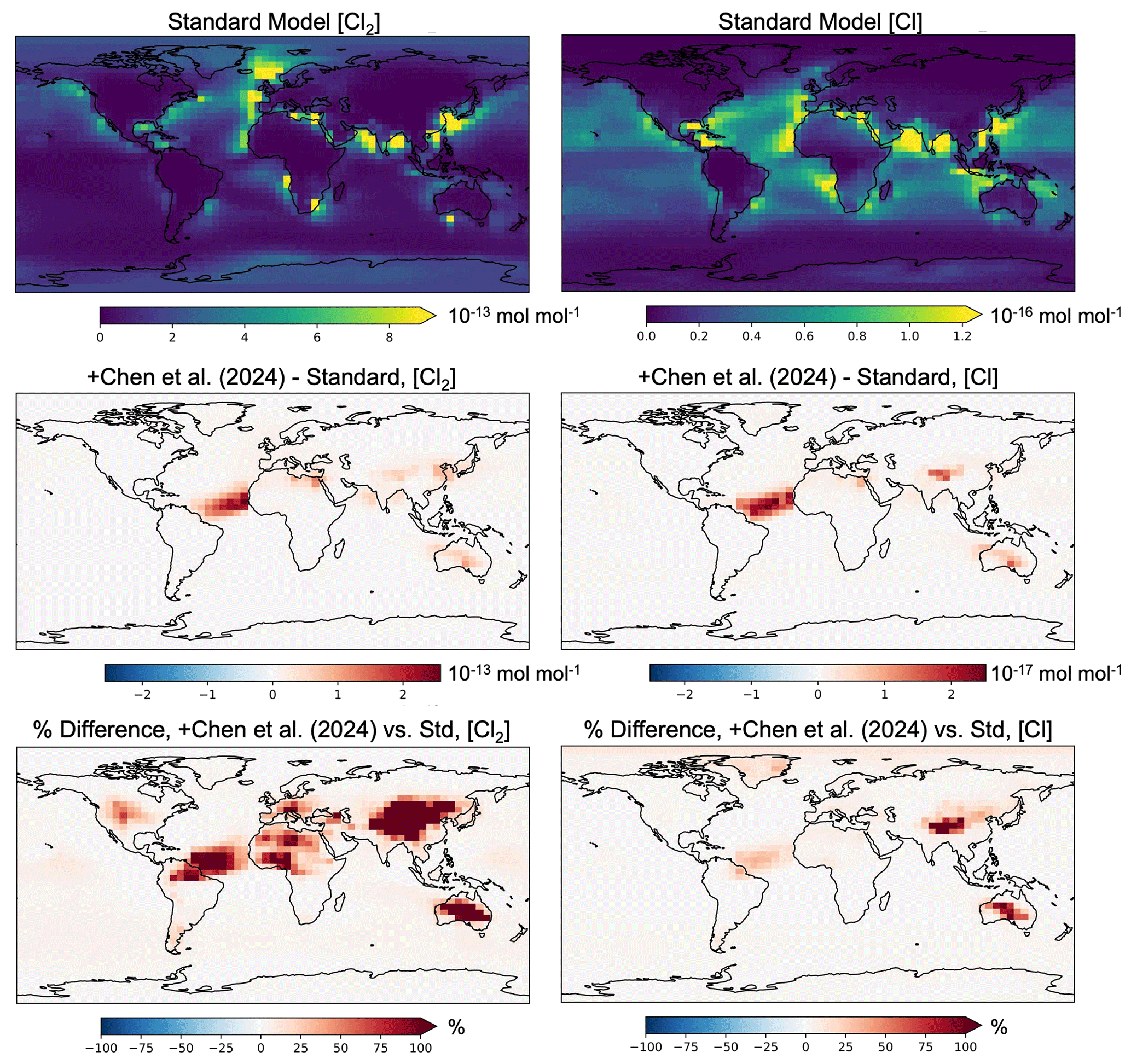
Figure 2 Impacts of adding natural Cl₂ emissions from the Chen et al. (2024) parameterization on simulated year 2019 annual mean surface-level concentrations of Cl₂ (left panels) and Cl (right panels). The top row is the standard model concentrations (mol mol⁻¹), with the second and third rows containing the absolute difference in mol mol⁻¹ and relative difference in percent, respectively, from adding the Chen et al. (2024) mechanism.

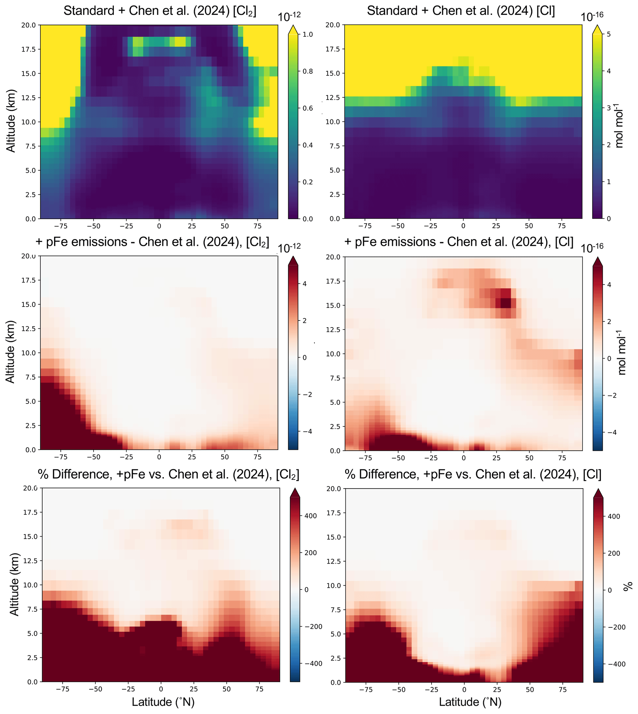
Figure 3 Impacts of adding surface pFe emissions (Iron experiment in Table 1) on simulated year 2019 zonal, annual mean concentrations of Cl₂ (left panels) and Cl (right panels) up to 20 km altitude. The top row is modeled concentrations in mol mol⁻¹ with the Chen et al. (2024) parameterization alone, with the second and third rows containing the absolute difference in mol mol⁻¹ and relative difference in percent, respectively, after pFe emissions are added to the surface layer in this simulation.

van Herpen et al. (2023) found that including their parameterization of Cl₂ release from mineral dust–sea spray aerosol (without any additional emissions) led to an increase in methane loss via the Cl atom of ∼ 20 %, although the overall global methane loss was decreased slightly due to a reduction in methane loss via reaction with OH. Here I find an increase in the tropospheric burden of Cl atom of 9.4 % (see Table 2) when the Chen et al. (2024) parameterization is included (without any additional emissions), which translates to an increase of 5.4 % in the methane loss via Cl atom. While van Herpen et al. (2023) do not report global changes in chlorine burdens, they find that total inorganic chlorine production is increased by 41 %. This led to a change in −0.7 % in the tropospheric ozone burden after including Cl₂ release from natural iron salt aerosol (van Herpen et al., 2023), while I find a change of −0.18 % in the tropospheric ozone burden when I include the Chen et al. (2024) parameterization. Thus, it is likely that the two parameterizations (see Table S3) result in Cl₂ production rates that are up to 4 times higher in van Herpen et al. (2023). In the zonal mean, increases in [Cl₂] and [Cl] from including the Chen et al. (2024) production mechanism are largest aloft (Fig. S4). van Herpen et al. (2023) limited their mechanism to the lower troposphere. Hence, differences in the vertical distributions of changes in chlorine vs. concentrations of ozone and methane in the two parameterizations may further contribute to the differences in impacts. The Chen et al. (2024) mechanism was evaluated directly against hourly observations of gas-phase Cl₂ in Wangdu, China, as well as key parameters including aerosol [Cl⁻], aerosol total iron, $j_{{\mathrm{NO}}_{\mathrm{2}}}$, and aerosol surface area (see Eq. 2). GEOS-Chem also captured the variability and magnitude of daily total Fe and Cl⁻ concentrations in fine-mode aerosol collected from 29 sites across North China, and slightly underestimated the observed solubility of aerosol Fe which was sampled at two sites, during the intensive study period at Wangdu (Chen et al., 2024). While adding the mechanism greatly improved the model performance of [Cl₂] at Wangdu, increasing simulated concentrations by a factor of 28 to 48, the modeled concentrations remained lower than those observed. Chen et al. (2024) hypothesized this may be due to overestimated aerosol water in the model's thermodynamic module and thus underestimated aqueous-phase [Cl⁻] and [Fe³⁺]. Low aerosol water content at high altitudes and hence high aqueous concentrations may explain the increases aloft seen in Fig. S4. It is outside of the scope of this paper to address uncertainties in the parameterization at higher altitudes. Figure 3 shows the annual mean change in Cl₂ and Cl atom concentrations in the Iron experiment (see Table 1) relative to the model with the Chen et al. (2024) mechanism alone, averaged zonally through 20 km altitude. Here, zonal mean increases in [Cl₂] and [Cl] due to iron emissions are largest near the surface (much greater than 400 %, up to 60 000 %) where emissions are added, unlike when the Chen et al. (2024) parameterization is included in the absence of additional surface emissions (Fig. S4). Figures 3 and S4 show that the additional release of Cl₂ due to natural or emitted iron leads to changes in Cl₂ and Cl that have differing spatial patterns and magnitudes in the annual mean due to physical and chemical processing. Tropospheric-wide differences between changes in Cl₂ and changes in Cl (see Table S5) are minor from adding the Chen et al. (2024) parameterization alone or in the Chloride experiment, but diverge most in experiments where iron emissions are added (Iron and Iron_Chloride). There, the relative increase in Cl₂ is 4 to 6.5 times greater than what is realized for Cl (Table S5).

With the parametrization used in this study, iron salt aerosol can lead to changes in steady-state methane of −5.4 % to +3.2 % depending on the emissions employed and their relative effects on Cl vs. OH (see Fig. 1). The Iron experiment led to a small decrease in steady-state methane (−1.7 %) from a tropospheric-wide factor of 2.7 increase in Cl atom (see Table S5). The Iron_Chloride experiment led to a larger decrease in steady-state methane (−5.4 %) due to a larger 7.6-fold increase in Cl atom burden, despite a much larger reduction in OH (−8.6 % vs. −2.1 %; see Tables 2 and S5). For a similar increase in Cl atom burden, emitting chloride (Chloride, 2.8-fold increase in Cl) instead of iron aerosol (Iron, 2.7-fold increase in Cl) led to a larger decrease in OH (−3.9 % vs. −2.1 %; see Table 2) and hence net increase in methane (+3.2 %). Li et al. (2023b) found that a 2.8-fold increase in Cl burden (from 88 Tg yr⁻¹ gas-phase Cl₂ emission) was insufficient to decrease methane, while a 7.9-fold increase in Cl burden (from 313 Tg yr⁻¹ gas-phase Cl₂ emissions) overcame the OH competition and led to a decrease in methane concentrations by about 6 % after 10 years (Li et al., 2023b). This suggests that the threshold of additional chlorine needed to overcome the OH limitation depends on what is emitted and the background chemistry in the model employed.

Here I find that emitting sea salt chloride along with particulate iron increases methane loss. This is a function of the formulation of the Chen et al. (2024) mechanism, which occurs on sea salt chloride aerosol and increases with increasing [Cl⁻] concentrations (see Sect. 2.2.2, “Implementation of Chen et al. (2024) iron salt aerosol mechanism”, and Eq. 2). Artificial chloride aerosol emissions in addition to the particulate iron emissions can replenish the sea salt chloride that was converted to Cl₂ and increase aerosol [Cl⁻] concentrations, leading to greater overall production of Cl₂ (see Table S5).

The iron emissions needed to decrease methane are also uncertain and sensitive to the mechanism and rate of chlorine release from iron salt aerosol. The Iron and Iron_Chloride scenarios presented here have 565 Tg yr⁻¹ iron emissions (see Table 1) leading to a decrease in steady-state methane of 1.7 % to 5.4 %. In a Community Earth System Model (CESM) study using the van Herpen et al. (2023) parameterization for chlorine release, additional iron emissions of 200 Tg yr⁻¹ (which increased Cl₂ production by ∼ 850 to 930 Tg yr⁻¹ depending on the region of emission) lead to a ∼ 20 % decrease in global methane concentrations after 10 years (Meidan et al., 2024). This study found that a threshold of at least 6 Tg yr⁻¹ of iron was needed in the most idealized setup to avoid increasing methane, though larger emissions of > 60 Tg yr⁻¹ of iron may be needed for significant methane reductions. In addition, the properties of the emitted iron would affect the amount of iron needed to increase Cl₂. Meidan et al. (2024) emitted combustion-type iron (initially 6 % soluble with 31.6 % of that as photoactive, with a parameterization allowing the conversion of insoluble to soluble iron), similar to my approach of emitting anthropogenic iron (here, 40 % soluble with 67 % of that as photoactive, see Sect. 2.2.2, “Implementation of Chen et al. (2024) iron salt aerosol mechanism”). Pure FeCl₃ may require less total mass due to its higher solubility and pure Fe(III) speciation.

Here, the methane loss in the Iron_Chloride scenario decreases in the tropical and southern hemisphere's free troposphere, with increases in methane loss rates limited mostly to the surface and some regions of the upper troposphere. There may also be a reduction in Cl₂ production from chloride via other reactions with OH and chlorine nitrate (ClNO₃) due to reductions in tropospheric OH and NO_x; thus, the representation of competing heterogeneous halogen chemical reactions may play a role in the predicted effectiveness of iron salt aerosol. Additional laboratory experiments and field observations are needed to constrain this process in natural and engineered aerosol mixtures.

Overall, OH-based scenarios and gas-phase emission of Cl₂ lead to significant decreases in steady-state methane but require extremely large emissions. Cl₂ is much more effective at reducing methane (−14.3 %) than hydrogen peroxide (−4.6 %) for the same level of emission (1250 Tg yr⁻¹). There are uncertainties in the exact impact on methane of a given amount of Cl₂ emission (e.g., in this study vs. Li et al., 2023b) due to a variety of factors including the representation of complex reactive halogen chemistry. Despite this, the methane lifetime and methane concentration reductions from 1250 Tg yr⁻¹ of gas-phase Cl₂ emissions presented here are qualitatively similar to those of Li et al. (2023b). In contrast, by using a different chlorine release mechanism from iron salt aerosol from Chen et al. (2024) and a different atmospheric model, I find that larger iron emissions (565 Tg yr⁻¹) than those used in Meidan et al. (2024) (200 Tg yr⁻¹) lead to a smaller decrease in methane (−1.7 % at steady-state vs. −20 % after 10 years). The mechanism of Cl₂ emission, whether this would also release bromine, and how fast the release from iron salt aerosol is will affect whether this method would decrease or increase steady-state methane.

3.3 Impacts on Other Climate Forcers and Ozone-Depleting Substances

GEOS-Chem simulates additional greenhouse gases and ozone-depleting substances including nitrous oxide (N₂O), halons (three species), hydrochlorofluorocarbons (HCFCs; four species), chlorofluorocarbons (CFCs; five species), and other halomethanes (12 species, e.g., chloromethane, methyl bromide, chloroform). I examined the changes in tropospheric burdens of each. Due to the short simulation length of 1 year following 1 year of initialization, I focus here only on short-lived species (lifetimes < 6 months).

Details of changes in tropospheric burdens (accounting for the temporally and spatially varying tropopause) for selected short-lived species with significant impacts from the AOE experiments are shown in Table S7. Of the short-lived halomethanes, bromoform (CHBr₃) and dibromomethane (CH₂Br₂) have the largest tropospheric-wide, with decreases in the hydrogen peroxide–based experiments and increases in the Cl-based experiments. Dichloromethane and chloroform follow the same pattern, but changes are smaller overall. For dibromomethane, dichloromethane, and chloroform, the addition of bromine in the Cl₂_BrCl_ Br₂ experiment leads to larger increases relative to Cl₂ only. These short-lived gases could contribute to ozone depletion in the stratosphere and are not regulated by the Montreal Protocol (e.g., Hossaini et al., 2017). Iodine-containing halomethane tropospheric burdens decrease across all experiments due to the reduction in overall I_y (Sect. 3.1), with the largest decreases seen for methyl iodide (CH₃I), which is not thought to contribute to stratospheric ozone loss (Zhang et al., 2020). The shortest-lived HCFC simulated by GEOS-Chem is HCFC-123 (atmospheric lifetime 1.3 years). One year of AOE leads to large changes in its tropospheric burden, with decreases in the hydrogen peroxide–based scenarios (up to −74 %) and increases in the Cl-based scenarios (up to 63 %). As HCFC-123 has a 100-year global warming potential of 90.4 (Smith et al., 2021) and is a class-II ozone-depleting substance, longer-term simulations are needed to fully quantify the climate impact of AOE. At the same time, tropospheric ozone decreases in all AOE experiments (see Table 2) which could lead to a negative radiative forcing. Full radiative transfer calculations would be needed to quantify the overall impact.

Across all experiments except Chloride, tropospheric inorganic aerosol increases (see Table S7) due to the increase in tropospheric sulfate and ammonium, partially offset by decreases in tropospheric nitrate burdens. This is likely due to the HOCl $/$ HOBr + S(IV) pathways that produce sulfate (Wang et al., 2021), as Br_y and Cl_y both increase in nearly all experiments. This is a departure from Li et al. (2023b), who found decreases in sulfate of ∼ 10 % from 1250 Tg yr⁻¹ Cl₂ emissions. This difference may reflect the coupled halogen-sulfate chemistry in GEOS-Chem (Chen et al., 2017; Wang et al., 2021) that does not appear to be included in the CESM chemical mechanism (see Table S2). For the hydrogen peroxide experiments, increased hydrogen peroxide and OH will also increase the oxidation of SO₂ to sulfate in the aqueous and gas phases, respectively. For the Iron and Iron_Chloride experiments, sulfate may also increase due to the Fe(III)-catalyzed pathway (Alexander et al., 2009). Partitioning of ammonium and nitrate aerosol is determined by the thermodynamic model ISORROPIA-2 in GEOS-Chem (see Sect. 2.1). Thus, ammonium likely concurrently increases to neutralize the excess sulfate in all experiments. For the Chloride experiment, decreases in nitrate and sulfate are nearly exactly offset by increases in ammonium. Nitrate is likely reduced due to reductions in NO_x in most experiments (see Table 2) and is influenced by the change in gas-particle partitioning due to increased sulfate production. Increases in the tropospheric inorganic aerosol burden could lead to an additional negative radiative forcing. Changes in these aerosols at the surface and the associated air quality implications are examined in Sect. 3.4.

3.4 Impacts on Surface Air Quality

Surface PM_2.5, CO, ozone, and NO₂ are air pollutants impacted by the atmospheric oxidation enhancement experiments. These largely follow the changes in tropospheric burdens (see Tables 2 and S6). Surface NO₂, however, was negligibly impacted by all experiments; most of the changes in tropospheric NO_x occurred in the upper troposphere (see Fig. S5). The change in global annual mean surface PM_2.5, CO, and ozone is shown in Fig. S6 across the different scenarios, with spatial variations in annual mean surface PM_2.5 and ozone shown in Figs. 4 and 5, respectively.

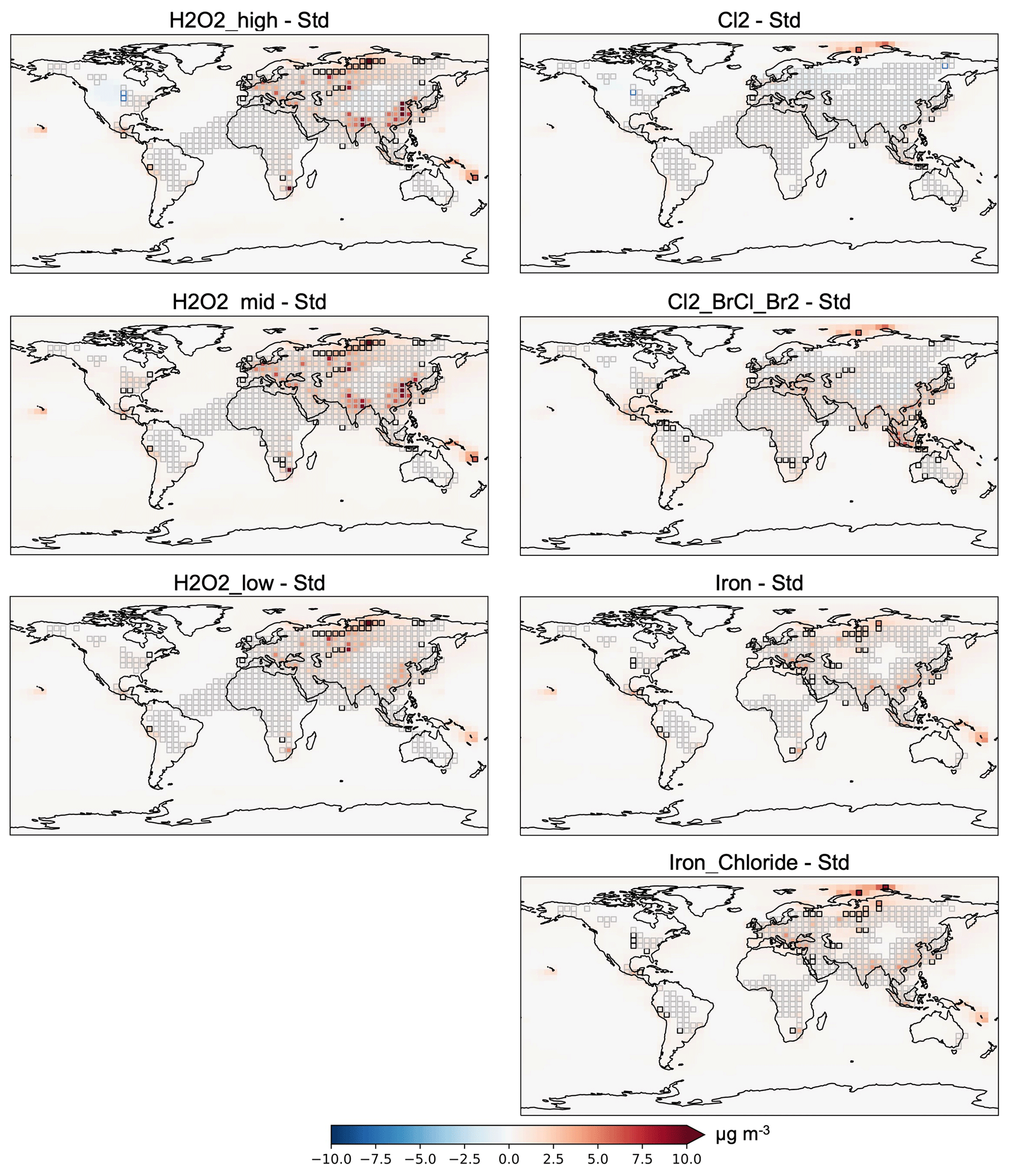
Figure 4 Absolute change in surface PM_2.5 relative to the standard model in year 2019. Gray boxes: areas already in exceedance of USEPA's annual mean PM_2.5 primary standard of 9 µg m⁻³, which remain in exceedance when the experiment is applied. Black boxes: the experiment brought a region from < 9 µg m⁻³ to an exceedance of ≥ 9 µg m⁻³. Blue boxes: experiment led to improved PM_2.5 from an exceedance to < 9 µg m⁻³.

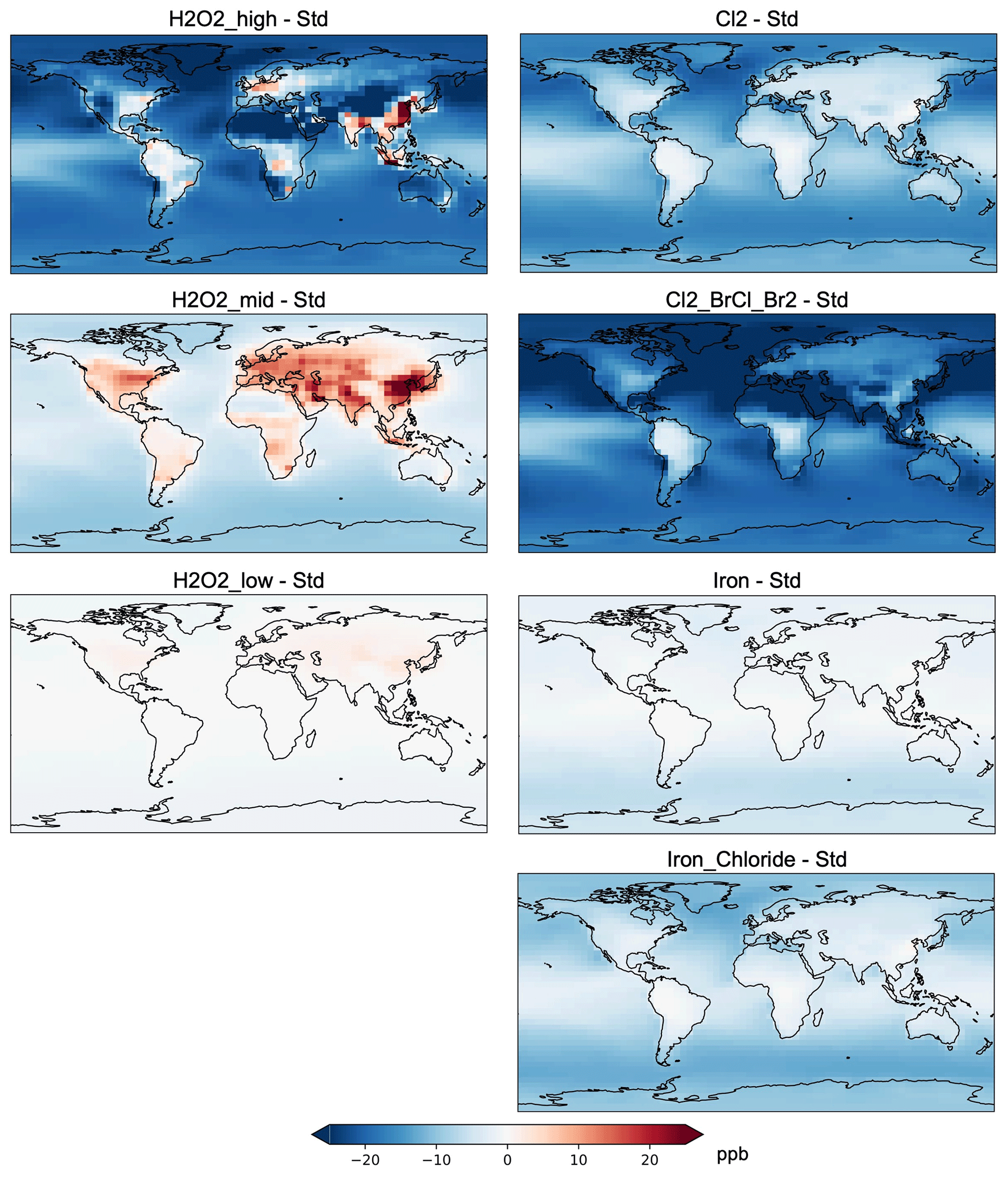
Figure 5 Absolute change in surface ozone (ppb) between model experiments detailed in Table 1 and the standard model in year 2019.

In the mean across all scenarios, there are declines in surface ozone air pollution (Fig. S6). Surface PM_2.5 increases in all scenarios except in the Chloride case, where in the absence of iron to mediate the Cl₂ release, the additional chloride leads to decreased sulfate and nitrate. Interestingly, H₂O₂_mid has worse air quality impacts than H₂O₂_high despite having less emissions; PM_2.5 increases more, and CO and ozone decrease less. There are larger impacts on PM_2.5 from the hydrogen peroxide and OH methods (up to 14–19 µg m⁻³ in an individual model gridbox) than the Cl₂ and Cl₂_BrCl_Br₂ methods (up to 6–7 µg m⁻³ in an individual gridbox). These results are consistent with prior work suggesting that aerosol production can be oxidant-limited (e.g., Mayhew and Haskins, 2025; Shah et al., 2018), and observational and model studies showing that long-term declines in sulfate aerosol are weaker than those of SO₂ on a global and regional scale due to increased SO₂ oxidation (e.g., Manktelow et al., 2007; Aas et al., 2019; Lin et al., 2025). Globally averaged, I find annual mean increases in PM_2.5 of 0 to 0.3 µg m⁻³ for Cl-based approaches and 0.3 to 0.4 µg m⁻³ for H₂O₂ experiments (see Fig. S6). Figure 4 shows the absolute change in PM_2.5 spatially in year 2019. Gray boxes highlight areas already in exceedance of the U.S. Environmental Protection Agency's (EPA's) annual mean PM_2.5 primary standard of 9 µg m⁻³, which remain in exceedance when the experiment is applied. Black boxes highlight areas where the experiment to increase methane oxidation brought a region from < 9 µg m⁻³ to an exceedance of 9 µg m⁻³. Blue boxes show where the experiment led to improved PM_2.5 from an exceedance to < 9 µg m⁻³.

These results represent one single year of AOE application (2019). As such, the exact magnitude and spatial patterns of changes in annual mean PM_2.5 due to AOE may vary interannually due to variability in meteorology and its effects on natural emissions, pollutant transport, and PM_2.5 removal, and the variability in background anthropogenic emissions. Moreover, long-term simulations using the CESM2 model suggest that relative changes in tropospheric sulfate aerosol and ozone due to Cl₂ gas-based AOE increase during the first 15 years of continuous application and then stabilize (Li et al., 2023b). Here, Fig. 4 highlights the potential risks in surface PM_2.5 air quality in different regions in the initial years of deployment. Although the emissions for Cl₂ and Cl₂_BrCl_Br₂ are focused over the oceans, there are larger changes seen on land in both cases than over the oceans – with the exception of the Arctic ocean, where ammonium aerosol drives a larger increase (Fig. 4). The largest absolute increases in surface PM_2.5 in the hydrogen peroxide experiments occur in Europe, India, China, Russia, Equatorial Asia, and southern Africa (Fig. 4). The impact of daytime-only emissions (not shown) varied depending on the level of hydrogen peroxide emissions; for the H₂O₂_mid scenario, daytime-only emissions had higher PM_2.5 concentrations, but for the H₂O₂_low scenario the daytime-only emissions reduced PM_2.5 concentrations. Similarly to the tropospheric-wide changes, these changes are driven by increases in sulfate with decreases in nitrate partially compensating, particularly in the Cl₂ and Cl₂_BrCl_Br₂ methods. Decreases in nitrate lead to small decreases in total PM_2.5 in some regions in the Cl₂ scenario. Overall, AOE exacerbates existing PM_2.5 air quality issues in populated regions of Europe and Asia in year 2019 (Fig. 4).

Figure 5 shows the absolute change in annual mean surface ozone across model experiments. In the global mean, surface ozone decreases on average in all methods (see Fig. S6), with largest mean decreases in the Cl₂_BrCl_Br₂ and H₂O₂_high experiments. At the same time, individual grid boxes in the hydrogen peroxide experiments see increases in annual mean ozone across populated areas (see Fig. 5). This has implications for the location of additional OH release, balancing the targeting of methane point sources versus populated areas where ozone may increase. Figure 5 again highlights that H₂O₂_mid has worse air quality impacts for ozone than H₂O₂_high.

Surface CO follows the tropospheric changes presented in Sect. 3.1 with decreases in hydrogen peroxide–based scenarios and increases in chlorine-based scenarios. Increases in surface CO concentrations in the chlorine-based scenarios are small relative to health guidelines and largely occur over the oceans. Surface CO decreases everywhere in the hydrogen peroxide–based experiments. These changes represent the short-term impact over 1 year of applied AOE.

4 Uncertainties

Model resolution. Here I use a coarse-resolution global model simulation. This is not appropriate to examine point source applications near high methane emitters. Model resolution can lead to biases due to nonlinear atmospheric chemistry. However, these effects vary spatially and temporally and for tropospheric NO₂ in GEOS-Chem are within ±8 % of high-resolution simulations (Li et al., 2023a). Resolution effects are most important in polluted regions and are becoming less important as anthropogenic sources are reduced (Li et al., 2023a). At the same time, Pennacchio et al. (2025) demonstrated the challenges in representing high-chlorine conditions in global lower-resolution models that result from point source emissions of iron for atmospheric methane oxidation enhancement, including how dilution of iron emission plumes and their interactions with the surrounding NO_x and ozone gradients can change the direction of the change in methane predicted. In this study, I emit species for the chlorine-based AOE experiments uniformly over all global oceans rather than in concentrated ship plumes. While coarse-resolution models may underestimate methane removal within these high-ClO_x plumes, Pennacchio et al. (2025) find that due to rapid dilution, iron salt aerosol released from ships would spend most of its atmospheric lifetime in a dilute, low-ClO_x regime, likely leading to an increase in methane over most of the global oceans after accounting for background NO_x and ozone levels.

Uncertainties in iron salt aerosol mechanism. Representation of chlorine release from iron salt aerosols in models remains highly parameterized. Complexities in iron solubility and speciation are not well represented. Depending on the reaction rate and representation, a given mass of iron salt aerosol release may lead to increases or decreases in the methane lifetime. Additional laboratory studies of natural and engineered iron salt aerosol, including mixtures with ambient species, are needed to improve the understanding of the kinetics and driving factors. Field studies and additional observations that could help evaluate this mechanism in models (e.g., isotopic composition, chloride, chlorine, iron and its speciation) will also aid in constraining this process.

Methods for OH release. The method and location of OH release will have different impacts. Here I only examined hydrogen peroxide as a mechanism for OH release, versus OH release without a specific mechanism. Effects of water vapor or artificial radiation for producing OH could have additional effects on climate forcers and air pollution.

Chemistry and time horizon. Here I use the “simple” SOA mechanism (fixed-yield, direct, and irreversible formation); additional simulations would be needed to better understand the change in SOA production under varying chemical regimes of OH and chlorine addition for methane oxidation. In addition, emissions are kept constant in year 2019. Most of the PM_2.5 effects predicted here are mediated by sulfate; future reductions in SO₂ emissions would likely limit this effect. We do not include interactive hydrogen (H₂) chemistry in our model simulation. Increased methane oxidation by OH in the hydrogen peroxide–based scenarios could lead to increased atmospheric H₂, as would potential future increases in hydrogen applications and their associated H₂ emissions from leakage. This would lead to a positive feedback on methane, as H₂ reacts with OH and reduces the amount of OH available to oxidize methane (e.g., Bertagni et al., 2022; Ocko and Hamburg, 2022; Warwick et al., 2023). As the simulations here are performed for only 1 year following 1 year of initialization, they cannot assess the stratospheric impact of AOE including on ozone depletion due to the long lifetime of air in the stratosphere. Over 30-year-long CESM2 simulations, Li et al. (2023b) find that chlorine-based AOE leads to stratospheric ozone depletion. The 1-year simulation also does not capture potential interannual variability in AOE effects due to meteorology or emissions. Finally, uncertainties in the representation of halogen chemistry may impact the prediction of unintended consequences. For example, whether the halogen chemical mechanism includes interactions with sulfur seems to lead to different results for how increased chlorine affects sulfate aerosol between this study (increases) and Li et al. (2023b) (decreases).

Fixed boundary condition for methane. Surface-level methane concentrations are fixed, including during the AOE model experiments, potentially affecting the predicted atmospheric chemistry impacts at the surface. However, given the long lifetime of methane, methane concentrations during the 1 year of simulated AOE decrease by < 1 % everywhere, including just above the surface layer and at other altitudes where OH (in H₂O₂ experiments) or Cl (in Cl-based experiments) increase by more than 100 %. As discussed in Sect. 2.1, the simplified surface representation does not impact estimates of changes in steady-state methane (e.g., Khodayari et al., 2015).

5 Conclusions

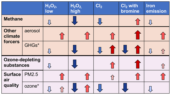
Here we simulate multiple scenarios of enhancing atmospheric methane oxidation via OH or Cl including hydrogen peroxide release, Cl₂ emissions, and iron salt aerosol in a global chemical transport model to assess the potential for decreasing the methane lifetime and resulting impacts on other climate forcers, stratospheric ozone, and surface air quality. The overall impacts of atmospheric oxidation enhancement methods on climate and human health involve multiple competing factors (see Fig. 6).

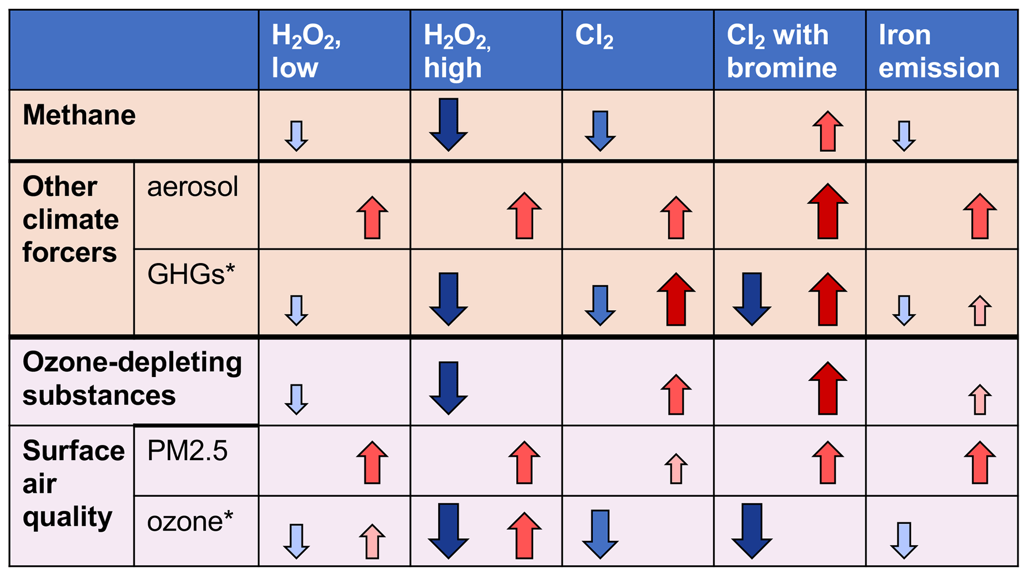
Figure 6 The overall impacts of atmospheric oxidation enhancement methods on climate and human health involve multiple competing factors. The color and size of arrows represents the approximate magnitude of change, with larger changes darker and larger arrows. Note: ^∗ = sign of change depends on species (greenhouse gases [GHGs]) or location (ozone).

Based on the present work, current global production of hydrogen peroxide is not sufficient to affect methane on a global scale, and this presents a challenge. Release of gas-phase Cl₂ is promising, but the exact mechanism to accomplish this and ensure it is large enough to reduce rather than increase methane remains a major challenge. Two different model approaches (this work, and Li et al., 2023b) show that a large quantity of Cl₂ (> 100–300 Tg yr⁻¹) must be added to the atmosphere in order to have an impact. Smaller amounts, or increasing particulate chloride as shown in this study, will increase methane. Here we find that emitting particulate iron alone to catalyze chlorine release from sea salt aerosol following the reaction rate parameterization from Chen et al. (2024) can release sufficient Cl₂ to decrease global methane by 2.5 % but requires larger emissions than in previous studies (565 Tg yr⁻¹) to accomplish a smaller change.

In addition to the impacts on methane, increased atmospheric oxidation via hydrogen peroxide- and chlorine-based methods largely has a climate co-benefit, via increased tropospheric aerosols and decreased tropospheric ozone. Chlorine-based methods increase other greenhouse gases and thus have reduced climate co-benefits.

Overall, ozone-depleting substances are increased in chlorine-based methods and decreased in OH-based methods. Most of the species impacted are short-lived. Longer simulations are needed to understand the full impacts on stratospheric chemistry.

Chlorine-based methods reduce surface ozone air pollution. OH-based methods largely result in ozone reductions as well but lead to increases in ozone in already polluted areas. Surface PM_2.5 pollution increases over land and in highly populated regions across most chlorine scenarios and all OH-based methods, regardless of whether emissions are limited to the oceans. These increases are on the order of present EPA air quality standards for annual mean PM_2.5. These results from a one-year simulation highlight potential risks to air quality during the initial phases of AOE deployment.

Co-emission of bromine with chlorine appears to remove any benefit from chlorine-based approaches. In the case of 20 % bromine release by mass with respect to chlorine, the methane lifetime increases by 6.7 %. The addition of bromine also generally results in worse outcomes with respect to surface air quality, halogenated greenhouse gases, and ozone-depleting substances. Additional experimental measurements of bromine species released from natural and engineered iron salt aerosol are needed to constrain these effects.

Overall, additional research in higher-resolution, longer-term modeling frameworks as well as laboratory experiments is needed to constrain whether the AOE methods have the desired intended consequences of sufficiently decreasing atmospheric methane, and the risk level for the unintended consequences of potential increases in halogenated greenhouse gases, ozone-depleting substances, and particulate matter air pollution.