Linking in-canopy chemistry to above-canopy O₃, BVOCs, and NO_x gas fluxes in the Amazon rainforest

The forest canopy is a distinct chemical and dynamical environment compared to the atmosphere above, characterised by natural emissions, deposition processes, and chemistry that vary with height. However, the role of in-canopy chemistry and its influence on above-canopy concentrations of ozone (O₃) and bi-directional exchange of natural compounds are necessarily simplified within large-scale models. Whilst canopy models have been applied to temperate forests, there are few studies in tropical forests. Here, we apply the FORCAsT v2 canopy column model to an Amazonian site. Simulation of the 2015 El Niño shows that biomass burning enhances O₃ flux into the canopy, increases oxidation chemistry and elevates O₃ deposition to vegetation. Sensitivity tests show sesquiterpenes enhance O₃ chemical loss from approximately 3 % of the total in-canopy losses to 10 %–15 %, but only marginally reduce the total canopy O₃ flux. Sesquiterpene canopy escape efficiency varies by 45 %–55 % across simulations, controlled by O₃ oxidation and vertical turbulence. For other biogenic volatile organic compounds (BVOCs), pool-dependent emissions demonstrate greatest variability in escape efficiency with environmental conditions (monoterpenes 84 %–95 %, isoprene 95 %). Average soil NO_x escape efficiency (40 %–50 %) is higher than many existing models suggest and exhibits a strong diurnal cycle that drives O₃ production, especially in the early morning, which may be important to consider in global atmospheric chemistry models. Overall, we highlight reactive BVOCs by inclusion of sesquiterpene emissions and reactivity as major sources of uncertainty in in-canopy chemistry and emphasise the critical role of turbulence in linking canopy processes to above-canopy atmospheric composition.

1 Introduction

The Amazon rainforest stretches across 7×10⁶ km² to form a vast “green ocean” of trees; a continuous canopy of leaves in all directions. This surface plays a pivotal role in tropospheric chemistry, functioning as a dynamic interface that emits biogenic compounds and exchanges trace gases with the atmosphere above (e.g., Covey et al., 2021; Schmitt et al., 2023). Its most significant contributions include biogenic volatile organic compounds (BVOCs) and soil-emitted nitric oxide (NO), both of which influence atmospheric composition and chemistry. These compounds participate in photochemical reactions that lead to the formation of ozone (O₃), a short-lived climate forcer that adversely affects human health and vegetation. At the same time, O₃ is a key component in maintaining the atmospheric oxidation capacity, thereby regulating the lifetimes of numerous trace gases like BVOCs and methane (CH₄). These processes contribute to the formation of secondary organic aerosols (SOA), which influence the Earth's radiative balance and climate system. Furthermore, the forest serves as a surface for the deposition of atmospheric constituents, transferring trace gases from the atmosphere to the ecosystem.

This pristine tropical forest is rapidly changing (Aragão et al., 2018). Human activities and associated climate change are transforming the once-uninterrupted landscape into one fragmented by fire and deforestation (Marengo et al., 2018; dos Reis et al., 2021). From these regions, urban and biomass burning pollution can be advected long distances, influencing the chemical environment far from the emissions source (Brown et al., 2022). In particular, when NO_x from biomass burning interacts with the rainforest's naturally high BVOC emissions, it enhances the formation of O₃ (Pacifico et al., 2015; Pope et al., 2020). Elevated O₃, once transported into the canopy, can enter plant leaves, inhibiting growth and reducing carbon sequestration, threatening the rainforest's productivity (Cheesman et al., 2024; Vieira et al., 2023). Understanding O₃ concentrations over forested landscapes requires knowledge on how the canopy controls release and uptake of BVOCs, their interaction with NO_x and the role of the canopy in removing O₃.

Whilst global models often represent atmosphere-biosphere chemical exchange as a deposition or emission at a single surface layer, below the closed canopy structure exists a chemically vibrant space, with both chemical and depositional transformations occurring before canopy emissions are released to the atmosphere. Beginning in the trunk space, NO emissions from the soil can saturate the lower canopy, reacting with low concentrations of O₃ transported from above (Visser et al., 2022). In the near-perpetual darkness of the closed canopy, this acts as a chemical loss of O₃ and converts NO to NO₂. As NO is transported vertically, it encounters increasing concentrations of O₃, VOCs, and their oxidation products, further converting NO to NO₂. Exchange fluxes of NO_x and O₃ with soils and trees were intensively studied in the Amazonian rain forest within the LBA project (Gut et al., 2002) confirming that the plant canopy reduces the escape of NO_x by consumption of NO₂ under the strong influence of stomatal control (Breuninger et al., 2013; Chaparro-Suarez et al., 2011; Gut et al., 2002). Since O₃ and NO₂ are, among several gases, subject to deposition in the canopy and at the soil surface, the canopy acts to reduce the amount of NO_x from the soil that escapes the canopy at the same time as removing O₃ (Ganzeveld et al., 2002b).

Canopy emission rates in global models are often modified by a species-specific canopy escape efficiency to represent removal within the canopy before release. For soil NO_x, Yienger and Levy (1995) derive a function based only on leaf area index (LAI) and stomatal area index (SAI) that implicitly assumes an NO:NO₂ ratio and no temporal variation. However, they highlight that chemistry occurring below the canopy can affect this ratio, and it remains an uncertainty in the parameterisation and assumed magnitude of deposition.

Similarly, O₃ losses within the canopy through deposition and chemistry are often highly parameterised, with chemistry neglected altogether or implicitly included within deposition schemes. At different sites, chemical loss is estimated to contribute anywhere from a minor fraction to 20 % of O₃ loss in the canopy (Makar et al., 1999; Rummel et al., 2007; Visser et al., 2021, 2022). In the Amazon, Rummel et al. (2007) cannot explain nighttime chemical losses with soil NO alone and assume a significant contribution from reaction with advected pollutants. Additional research suggests an important role of sesquiterpenes in removing O₃ within the canopy (Isaacman-VanWertz et al., 2024; Jardine et al., 2011; Stroud et al., 2005). These highly reactive BVOC emissions have been measured in the Amazon, with both leaf and soil sources (Bourtsoukidis et al., 2018; Jardine et al., 2011) but are not regularly included in chemistry transport models due to their high reactivity and limited understanding of their chemical products. As these species are considered key to representing the biogenic chemical environment, some studies have included simple sesquiterpene mechanisms (Zhang et al., 2022).

Studies have proposed that accurate representation of NO_x and O₃ chemistry within the canopy is only possible with explicit canopy resolution. Especially in the tropics, strong gradients in trace gas vertical profiles are formed from low turbulence, allowing stable separation from the boundary layer overnight and in the trunk space (Chamecki et al., 2020; Freire et al., 2017; Serra-Neto et al., 2021). Stratification and the formation of microclimates can further cause processes to deviate from parameterisations. Makar et al. (2017) suggest gradients in light and turbulence within the canopy can reduce above-canopy O₃ concentrations by 12 %. Similarly, Visser et al. (2021) find single-layer schemes currently employed by land surface models misrepresent diurnal variability and stomatal : non-stomatal partitioning of O₃ sinks due to missing effects from turbulence. These studies find that only a few layers are needed to improve simulations, suggesting multilayer canopies could be implemented more frequently in global models in the future (Ganzeveld et al., 2002a; Makar et al., 2017; Vermeuel et al., 2024; Wang et al., 2025).

To prioritise development for large scale models, an overview of the factors affecting canopy escape efficiencies and O₃ removal within the tropical forest is required. This includes understanding the role of the above-canopy atmosphere in affecting processes below the canopy, for example through propagation of vertical turbulence or in response to upwind transport of precursors, as well as explicit quantification of the importance of chemistry below the canopy. This study evaluates the role of the canopy in controlling atmospheric composition within and above the Amazon forest using a resolved canopy column model. We compare a year with typical meteorology to one with more extreme conditions including higher fire activity to understand the role of transported pollution on O₃ removal, BVOC escape efficiency and soil NO_x escape efficiency compared to pristine conditions. This acts as a first step towards identifying the important features of trace gas exchange required for improved representation of tropical forest in-canopy processes and interactions in global models.

2 Methods

2.1 Observation data at the Amazon Tall Tower Observatory

We use the Amazon Tall Tower Observatory (ATTO) site (Andreae et al., 2015) as the location for study and evaluation of the column model. The site is a research facility within the Uatuma Sustainable Development Reserve, in the pristine Brazilian Amazon, 150 km NE of Manaus city (2° S, 59° W). This location is predominantly upwind of the city, although SE–E wind can bring pollution from biomass burning and agriculture, especially during the dry season (Pöhlker et al., 2019). The wet and dry seasons occur during December–May and July–October, respectively, while November and June are considered transition months. Daylight hours are 06:00 to 18:00 LT (UTC-4). The vegetation is old-growth forest, with an average canopy height of 35 m and greatest leaf density around 25 m (Gomes Alves et al., 2023).

Figure 1a summarises the ATTO measurements used in this study as driving data and for model evaluation. Measurements were taken at various heights along the 80 m tower (named the Instant tower, 2.1468° S, 59.0068° W), which has been in operation since 2012. Temperature, photosynthetically active radiation (PAR), friction velocity (u_∗), and wind speed and direction measurements are available continuously since 2012 in half-hourly intervals. Relative humidity (RH) in 2013 is also used for model evaluation.

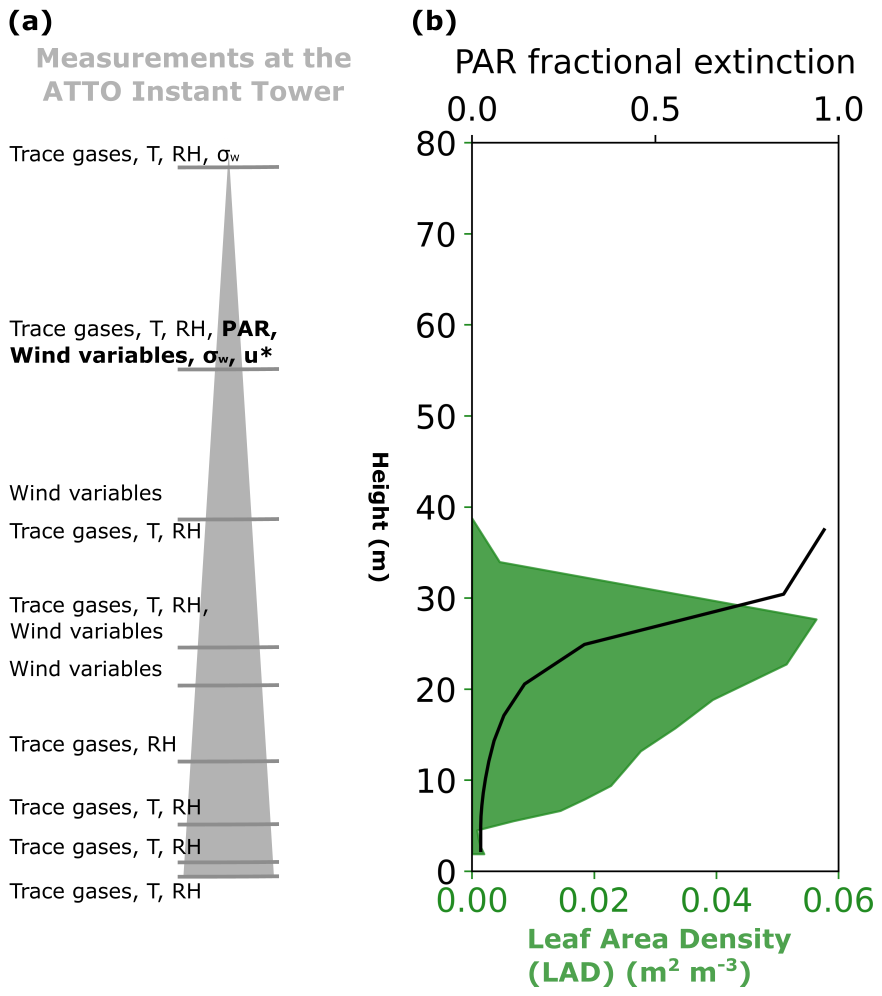
Figure 1 (a) The observed variables used for model evaluation throughout this paper and their approximate measurement heights. Variables measures are trace gases, temperature (T), relative humidity (RH), vertical wind standard deviation (σ_w), photosynthetically active radiation (PAR), friction velocity (u_∗) and wind speed and direction (wind variables). Variables in bold are used as driving data in the simulations, (b) prescribed leaf area density (green shading) and fractional extinction of PAR (black solid line) within the canopy (model simulated average). The height scale on both figures is the same.

Column model simulations (see Sect. 2.2) of the ATTO site require forcing data of vertical wind standard deviation (σ_w), u_∗, PAR, and wind direction which control mixing, temperature and light-related processes. Data from 1–13 November 2013 and 11–23 November 2015 are used in this study; these time periods were selected for maximum meteorological and chemical data availability. Vertical wind standard deviation is not continuously available at the site and was not recorded during 2013. Above-canopy observations are available from an intense campaign in 11–23 November 2015 at 55 and 81 m. In-canopy observations of σ_w were also measured at 24 m in a shorter period from 11–18 November 2015 (Dias-Júnior et al., 2019).

November 2013 reflects typical background conditions at ATTO, with moderate temperatures, clean air masses, and biogenic-dominated chemistry, whereas November 2015 represents a perturbed regime characterised by El Niño-driven warming, biomass burning influence, and enhanced atmospheric oxidation (Ribeiro Neto et al., 2022; Silva Junior et al., 2019). Consequently, 2013 observations are representative of the broader atmosphere–biosphere exchange during this period, while 2015 is used to investigate how climate extremes and fire activity may shift the chemical regime. Indeed, November 2015 may be more representative of dry season conditions.

To evaluate trace gases in our simulations, we compare model output to observed O₃ concentration measurements taken at the Instant tower during November 2013 and 2015. This profile setup measures at 8 heights using a TEI 49i O₃ analyser (Fig. 1a). The lower part of the vertical profile (0.05, 0.5 and 4 m above the forest floor) was set up on a tripod adjacent to the Instant tower. The upper part of the vertical profile (12, 24, 38, 53 and 79 m) was mounted on the tower. Tubes were guided to a valve system switching every 2 min between the different heights during the first three cycles within each hour, and every 1 min and 30 s during the last cycle, resulting in four measurements at each height per hour. The O₃ limit of detection (LOD) is 0.5 ppbv in 60 s. There are no O₃ flux measurements available for the simulation period so subsequent evaluations only consider O₃ concentration measurements.

Isoprene, monoterpenes (unspeciated) and isoprene oxidation products (MACR, MVK, ISOPOOH) were measured during 5 short campaigns from 2012 to 2015 (Yáñez-Serrano et al., 2015). Measurements were performed with a PTR-MS (Ionicon Analytic GmbH, Austria) operated under standard conditions using the same profile set up as above (Fig. 1a). As the closest time periods to that of our simulation, we use data from the campaigns in October 2015 and November 2012 as an observational reference to compare to November 2015 and 2013, respectively. Sesquiterpenes have not been measured at the site.

2.2 Model description and application to the ATTO site

We employ the FORCAsT v2 model (Ashworth et al., 2015; Wei et al., 2021), a multi-layer column model with explicit canopy representation originally developed for the University of Michigan Biological Station (UMBS) site. Our set-up includes 18 canopy layers of increasing height, 20 soil layers, and an additional 22 above-canopy layers extending to 5 km. The model timestep is 1 min with output archived every 30 min. The model is forced by observations at 30 min intervals of wind direction, σ_w, u_∗ and PAR recorded above the canopy (Figs. S1 and S2 in the Supplement). All other variables including temperature, wind speed, chemistry, water and energy fluxes are prognostic variables in the model after specifying initial conditions. The minimal number of forcing variables is a feature of this canopy model, since many other canopy chemistry models are nudged by above-canopy observations. Nudging gradually forces model variables towards observations and is commonly applied to constrain above-canopy long-lived gas concentrations and meteorology. This has the advantage of holding the above-canopy environment as close to the true values as possible, which enables evaluation of atmosphere-biosphere fluxes in response to above canopy changes, such as advection. Additionally, the below-canopy environment is more likely to be well-represented and analysis can focus on below-canopy processes. However, as nudging is a correction rather than an explicit representation of transport, it can mask transport or chemistry errors in the model. To represent lateral transport of air masses in a process-based way, FORCAsT v2 includes an advection parameterisation as a prescribed tendency inside the column. The advection parameter is adjusted to best reproduce observations of trace gas concentrations. The model is described in detail by Ashworth et al. (2015), Wei et al. (2021) and Bryan et al. (2012). We provide an overview of the model here, and modifications for our application at a tropical site; simulation details and the results can be found in Sect. 2.3 onwards.

The resolved canopy allows vegetation processes to be computed at each canopy layer. Leaf Area Index (LAI; m² leaf area per m² ground area) is specified at each layer and PAR is prescribed at the top of the canopy from observations. Canopy structure and radiative transfer properties are specified using parameters to describe the leaf angle distribution and response to incoming radiation (including absorption, reflection and thermal properties). Each layer is divided into 9 sunlit leaf angle classes and a shaded leaf class, with fractions in each class determined by canopy structure, zenith angle and LAI. Radiation transfer to each layer is calculated using the CUPID model scheme (Norman, 1979) allowing calculation of an energy budget. Leaf temperature, latent and sensible heat fluxes are prognostic variables at each layer and for shade and sun leaves in each leaf angle class.

For ATTO, LAI (=5.3 m² m⁻²) and its vertical distribution at each layer is taken from November 2015 measurements by Gomes Alves et al. (2023) (Fig. 1b). Variability in LAI at this site is not considered statistically significant (Botía et al., 2022). For leaf and canopy parameter values where there are no observations for the tropics, parameters are left in their default state.

2.2.1 Emissions

Biogenic emissions are calculated at each layer for each leaf angle class based on PAR (Fig. 1b) and prognostic leaf temperature of each leaf angle class, and scaled to each layer using LAI in each class.

Synthesis emission fluxes (F; $\mathrm{nmol}{\mathrm{m}}^{-\mathrm{2}}{\mathrm{s}}^{-\mathrm{1}}$) are calculated by Eq. (1):

$$\begin{array}{}\text{(1)}& F=\text{LAI}\times \mathit{\epsilon }s\times {\mathit{\gamma }}_{\text{TS}}\times {\mathit{\gamma }}_{\text{LS}}\end{array}$$

where εs is the light-dependent emission factor at standard conditions of 30 °C and incoming PAR of 1000 $\mathrm{\mu }\mathrm{mol}{\mathrm{m}}^{-\mathrm{2}}{\mathrm{s}}^{-\mathrm{1}}$, and γ_TS and γ_LS are scaling factors accounting for the leaf surface temperature and radiation to the leaf. The expressions for γ_LS and γ_TS are provided in Ashworth et al. (2015) and Guenther et al. (2012).

Pool emission fluxes (F; $\mathrm{nmol}{\mathrm{m}}^{-\mathrm{2}}{\mathrm{s}}^{-\mathrm{1}}$) are calculated using Eq. (2):

$$\begin{array}{}\text{(2)}& F=\text{LAI}\times \mathit{\epsilon }p\times {\mathit{\gamma }}_{\text{TP}}.\end{array}$$

The temperature-dependent pool emission factor εp (temperature=30 °C) is scaled by γ_TP to in response to the leaf surface temperature following Guenther et al. (1995) and described in Ashworth et al. (2015). Species-specific parameter values for the γ functions are as described in Guenther et al. (2012), including the β parameter for temperature dependence (Table 1).

Table 1 Emission factors used in the simulations for synthesis (εs) and pool (εp) emissions selected from sensitivity tests and the β temperature parameters from Guenther et al. (2012).

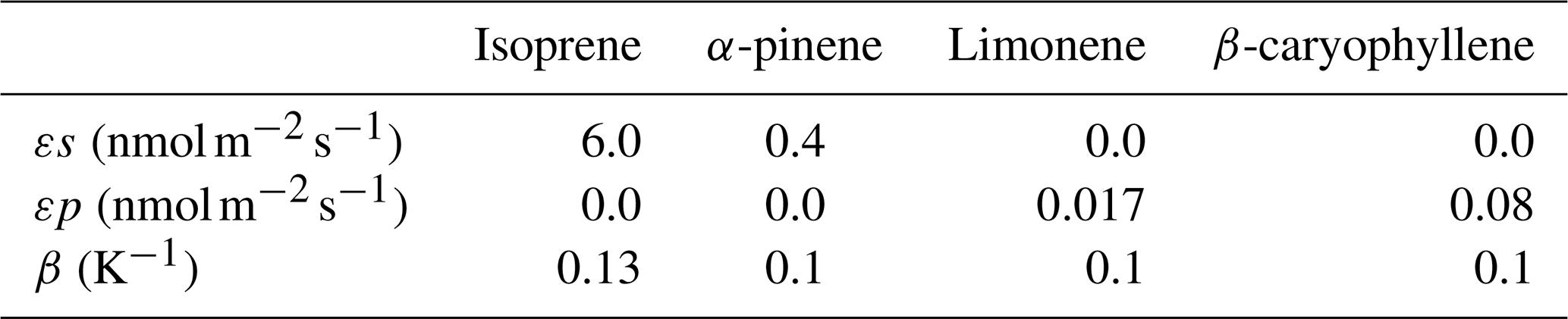
To select the εs and εp parameter values at the ATTO site we run 3 d sensitivity studies (Table S1 in the Supplement). The short-duration simulation is in-line with previous uses of the model, which were limited to 2 d. The details of the sensitivity tests and comparison to literature are shown in the Supplement (Figs. S3–S5), with the final parameters included in Table 1. As sesquiterpene emissions are highly uncertain and have the largest impact on O₃ concentrations, we test their contribution to chemistry further in the main simulations below (Sect. 2.3).

We set the light-dependent emission factor of isoprene to 6 $\mathrm{nmol}{\mathrm{m}}^{-\mathrm{2}}{\mathrm{s}}^{-\mathrm{1}}$ to reproduce observed maximum half hourly emissions of 6–10  $\mathrm{mg}{\mathrm{m}}^{-\mathrm{2}}{\mathrm{s}}^{-\mathrm{1}}$ at ATTO (Gomes Alves et al., 2023). Other BVOCs (monoterpenes and sesquiterpenes) do not have measured emission fluxes in the Amazon so emission factors must be estimated based on concentrations. We represent α-pinene as a light-dependent species (Kuhn et al., 2004a, b) and limonene as a temperature-dependent species based on observations at the ATTO site by Yáñez-Serrano et al. (2015), although the light and temperature dependence of tropical species emissions is currently not well characterised. Sesquiterpenes are emitted as 100 % β-caryophyllene, given the currently limited understanding of these BVOCs. Sesquiterpenes are considered pool emissions, and the temperature-dependent emissions factor is set at 0.08 $\mathrm{nmol}{\mathrm{m}}^{-\mathrm{2}}{\mathrm{s}}^{-\mathrm{1}}$ at 25 °C to match observed concentrations from Jardine et al. (2011) (Fig. S3). These measurements were taken at the nearby TT34 tower (2° S, 60° W) in the Amazon in 2010 (Jardine et al., 2011) as there are currently no tree- or leaf-level sesquiterpene measurements available at the ATTO site. Recent measurements at the ATTO site indicate that soils and cryptogams are very likely an additional source of sesquiterpenes (Bourtsoukidis et al., 2018; Edtbauer et al., 2021).

Terpenoids react with oxidants NO₃, O₃ and OH; isoprene dominates OH reactivity due to its abundance and some sesquiterpenes demonstrate high reactivity with O₃. Comparison of diurnal cycles of OH reactivity at 80 m to observations in 2018 by Pfannerstill et al. (2018) show the daily variability of OH reactivity is captured by the model, but the model underestimates the magnitude by 5–10 s⁻¹, likely because we do not include a full suite of BVOCs and the simulation length prevents oxygenated products from accumulating (Fig. S6). β-caryophyllene is one of the most reactive sesquiterpenes with respect to O₃ and it is often measured to be among the most abundant (e.g., Costa et al., 2025; Gomes Alves et al., 2022; Jardine et al., 2011). Thus, by including only this species of sesquiterpene our results represent an upper limit on sesquiterpene O₃ reactivity.

Soil NO emissions are temperature-dependent (Forkel et al., 2006) such that the emission factor (0.02 $\mathrm{nmol}{\mathrm{m}}^{-\mathrm{2}}{\mathrm{s}}^{-\mathrm{1}}$) is scaled by an exponential dependency on the top layer soil temperature (β):

$$\begin{array}{}\text{(3)}& \mathit{\beta }=e^{\mathrm{0.071}\cdot T\left(\mathrm{°}\mathrm{C}\right)}.\end{array}$$

Observed soil NO emission fluxes in undisturbed tropical forests span a large uncertainty range from 3 to 100 $\mathrm{\mu }\mathrm{g}{\mathrm{m}}^{-\mathrm{2}}{\mathrm{h}}^{-\mathrm{1}}$ (Bakwin et al., 1990; Erickson et al., 2002; Lee et al., 2024; Rummel et al., 2002). Most models of soil NO estimate values of 3–7 $\mathrm{\mu }\mathrm{g}{\mathrm{m}}^{-\mathrm{2}}{\mathrm{h}}^{-\mathrm{1}}$ (Yan et al., 2005; Yienger and Levy, 1995) for tropical soils. We select an emission factor of 0.02 $\mathrm{nmol}{\mathrm{m}}^{-\mathrm{2}}{\mathrm{s}}^{-\mathrm{1}}$ for an average emission of 9 $\mathrm{\mu }\mathrm{g}\mathrm{N}{\mathrm{m}}^{-\mathrm{2}}{\mathrm{h}}^{-\mathrm{1}}$ following sensitivity tests described in the Supplement (Fig. S7). This is at the upper end of previously simulated ranges (Hudman et al., 2012; Yienger and Levy, 1995) as suggested by Lee et al. (2024) but towards the lower end of the large range in observed NO emissions from tropical soils (Lee et al., 2024). Sensitivity tests considering the effect on NO_x concentrations in comparison to observations at other tropical locations is included in the Supplement (Fig. S7).

NO emission fluxes and their sensitivity to driving variables remains a significant uncertainty. Global studies indicate increased emission with temperature (Ke et al., 2022; Luo et al., 2013), however studies on isolated tropical soils tend to show weaker temperature dependence (Cárdenas et al., 1993). Water status is also likely a driving factor of soil NO emission, with limited NO fluxes in water-logged or dry soils and heavy rainfall triggering NO emission pulses (Yienger and Levy, 1995), which is not considered here. There was no rainfall during the simulation periods (Sect. 2.3).

2.2.2 Deposition

Deposition is calculated using a Wesely (Wesely, 1989) resistance scheme, which includes boundary layer (R_b), cuticular (R_cut), mesophyll (R_mes) and stomatal (R_stom) resistances at each layer.

Boundary layer resistance follows Gao et al. (1993):

$$\begin{array}{}\text{(4)}& R_{\mathrm{b}}={\displaystyle \frac{\mathrm{0.05}\times (\frac{\text{lw}}{U}{)}^{\mathrm{0.5}}}{D}}\end{array}$$

where lw is the leaf width (0.05 m) and D is the ratio of the gas molecular diffusivity to the molecular diffusivity for water.

Cuticular conductance is scaled for each gas type using Henry's law constant (H) and reactivity relative to ozone (f₀):

$$\begin{array}{}\text{(5)}& R_{\text{cut}}={\displaystyle \frac{R_{\text{cut0}}}{H^{-\mathrm{5}}+f_{\mathrm{0}}}}.\end{array}$$

Using R_cut0=1000 s m⁻¹.

Mesophyll resistance is described using the same predictors:

$$\begin{array}{}\text{(6)}& R_{\text{mes}}={\displaystyle \frac{\mathrm{1}}{\frac{H}{\mathrm{3000}}+\mathrm{100}{f}_{\mathrm{0}}}}.\end{array}$$

Stomatal conductance uses a Jarvis-type scheme (Jarvis, 1976), which scales a minimum resistance based on empirical sensitivities to meteorological drivers:

$$\begin{array}{}\text{(7)}& R_{\text{stom}}=R_{\text{min}}\times f\left(T\right)\times f\left(\text{PAR}\right)\times {\displaystyle \frac{f\left(\text{VPD}\right)}{f\left(\mathit{\psi }\right)}}\end{array}$$

where temperature (T), PAR, vapour pressure deficit (VPD) and water potential (ψ) are calculated for each layer and leaf angle class, using R_min=120 s m⁻¹ for H₂O (and scaled by D for each gas). These parameter values are in-line with literature and observed values (e.g., Clifton et al., 2023).

Deposition to soil follows Gao et al. (1993) with an additional dependence on surface soil moisture (SM) that rapidly increases resistance in water-logged soils (Eq. 9), described in Ashworth et al. (2015):

$$\begin{array}{}\text{(8)}& R_{\text{gi}}={\left({\displaystyle \frac{H}{R_{\text{gs}}}}+{\displaystyle \frac{f_{\mathrm{0}}}{R_{\text{go}}}}\right)}^{-\mathrm{1}}\end{array}$$

where R_gs is gas solubility-controlled uptake (=500 s m⁻¹) and R_go is surface reactivity uptake (=200 s m⁻¹). In wet soil (SM>0.8):

$$\begin{array}{}\text{(9)}& R_{\text{go}}=\mathrm{200}-a(\text{SM}-\mathrm{0.8}).\end{array}$$

Using coefficient a=1800 s m⁻¹.

Aerodynamic resistance (R_a) at the lowest level height z is defined as:

$$\begin{array}{}\text{(10)}& R_{\mathrm{a}}={\displaystyle \frac{z}{K}}.\end{array}$$

These are combined to give a total surface resistance (R_g):

$$\begin{array}{}\text{(11)}& R_{\mathrm{g}}=R_{\mathrm{a}}+R_{\text{gi}}.\end{array}$$

The total deposition velocity (v_d) at each layer is transformed into a sink tendency ($S_{\text{dep}}=-\frac{v_{\mathrm{d}}}{z}c$ (s⁻¹)) using the layer trace gas concentration c and combined with the emissions tendency before being passed to the vertical transport solver (described below).

2.2.3 Advection

A basic advection scheme must be included for input of nearby heat and trace gas sources since 1-D models do not simulate horizontal atmospheric transport. There is insufficient data at this remote forest site to reliably include a complete mass-balance advection scheme, so FORCAsT v2 includes a simple parameterisation based on wind speed and direction developed by Bryan et al. (2012). The advection rate in ppbv s⁻¹ is proportional to wind speed (U; m s⁻¹) scaled by a coefficient k. The calculation of the U profile from observed u^∗ is described in the Supplement (Supplementary model description).

For the ATTO site, we investigate the inclusion of advection of NO₂ from biomass burning to heights 73–200 m when the wind direction comes from 90–150°. Biomass burning during the southern Amazon dry season (August–October) mostly occurs in the Arc of Deforestation in the E–SE Amazon border, a location named for the agriculture, logging and infrastructure expansion that occurs. Measurements at a site close to ATTO have identified increases of NO₂ coincident with increases in black carbon, attributed to biomass burning transport from this region (Cordova et al., 2004). Furthermore, back trajectories from HYSPLIT show airmasses to the ATTO site arriving from 90–150° often originate from biomass burning locations (Pöhlker et al., 2018). Although NO₂ was not measured, Pöhlker et al. (2018) identify clear increases in biomass burning aerosol when winds arrive from these directions during months August–November. Although November is considered a transition month, biomass burning in the Arc of Deforestation sometimes still occurs. We select a value of k that best improves representation of observed O₃ concentrations in 2015 ($k=\mathrm{2}\times {\mathrm{10}}^{-\mathrm{6}}$ ppbv m⁻¹). The inclusion of upwind transport of NO₂ by advection in 2015 is explored further in the main simulations below (Sect. 2.3).

2.2.4 Chemistry

FORCAsT v2 incorporates 576 chemical reactions involving 411 species. As in Wei et al. (2021), our simulations use the Caltech Atmospheric Chemistry Mechanism 3 (CACM3) with the Reduced Caltech Isoprene Mechanism (RCIM; Wennberg et al., 2018) to describe isoprene oxidation under low-NO_x conditions. Simple sesquiterpene chemistry is represented using β-caryophyllene oxidation by O₃, OH and NO₃ as a proxy for all sesquiterpenes (Table S2), with reactivity dominated by O₃. These reactions form a number of oxidation products including various peroxy radicals, HCHO, lumped organic acids, ketones and aldehydes, which continue to react with oxidants, NO, HO₂ and, in some cases, undergo UV photolysis (Wei et al., 2021). However, the reactivity and product formation from sesquiterpenes is highly uncertain due to lack of measurements. All gas species concentrations are calculated prognostically. O₃ concentrations (mol mol⁻¹) are initialised at heights z based on observations up to 79 m and extrapolated and bounded by a maximum concentration of 50 ppbv above 2000 m as in the following:

$$\begin{array}{c}{\displaystyle }\mathrm{2.0}\times {\mathrm{10}}^{-\mathrm{9}}+(z\times \mathrm{0.15}\times {\mathrm{10}}^{-\mathrm{9}})\text{: }z\le \mathrm{37}\mathrm{m}\\ {\displaystyle }\mathrm{10}\times {\mathrm{10}}^{-\mathrm{9}}+(z\times \mathrm{0.03}\times {\mathrm{10}}^{-\mathrm{9}})\text{: }\mathrm{37}\mathrm{m}<z\le \mathrm{2000}\mathrm{m}\\ \text{(12)}& {\displaystyle }\mathrm{50}\times {\mathrm{10}}^{-\mathrm{9}}\text{: }\mathrm{2000}\mathrm{m}<z.\end{array}$$

We initiate the simulation at midnight UTC, 20:00 LT; at this time most trace gas concentrations are low and do not need to be initialised.

2.2.5 Transport and fluxes

The mass flux for gas-phase species is described by Eq. (13):

$$\begin{array}{}\text{(13)}& {\displaystyle \frac{\partial c}{\partial t}}={\displaystyle \frac{\partial }{\partial z}}\left(K{\displaystyle \frac{\partial c}{\partial z}}\right)+S_{\mathrm{c}}\end{array}$$

where c is the mixing ratio of a chemical species, S_c represents the sum of emissions, deposition, and advection tendencies at each layer (s⁻¹), and K is the eddy diffusivity coefficient (m² s⁻¹).

Emissions, deposition and advection contributions are summed for each layer to calculate the rate of change (S_c) at each layer and are passed to the vertical transport solver. Numerically, these tendencies are incorporated through operator splitting: the term S_cΔt is added to the right-hand side before the implicit vertical transport solve. The chemical solver is applied subsequently. This operator splitting is described and evaluated in Wei et al. (2021).

In this version, we move soil NO emissions from being a lower boundary condition to an emission contributing to S_c in the lowest atmosphere layer. Surface emissions and deposition are therefore treated explicitly within the chemical source terms prior to the transport step. To ensure that turbulent transport redistributes species within the column without introducing additional sources or sinks at the domain boundaries, the transport solver applies zero-flux (Neumann) boundary conditions at both the lower and upper boundaries. At each timestep, new concentrations of all chemical species are calculated at each level using an implicit method to solve the partial differential equations required in calculation of mixing. The zero-flux upper boundary means there is no representation of entrainment but O₃ concentrations in our simulations equilibrate within a day to 20 ppb at 1 km and 50 ppb at 3 km and remain stable. As this is the first time the model has been used to simulate a longer time period without nudging (Otu-Larbi et al., 2021), improvement of the upper boundary concentrations should be considered in future.

Temperature is initialised below the canopy using a linear fit between the measured ground and canopy height temperatures. Above the canopy, initial temperature is extrapolated from the canopy level measurement using a prescribed lapse rate. Fluxes of heat at each layer are as follows:

$$\begin{array}{}\text{(14)}& {\displaystyle \frac{\partial T}{\partial t}}={\displaystyle \frac{\partial }{\partial z}}\left(K{\displaystyle \frac{\partial T}{\partial z}}\right)+S_{\mathrm{h}}.\end{array}$$

S_h represents sources and sinks of heat (K s⁻¹), such as from vegetation. Equation (14) is solved at each model layer to give prognostic temperature using surface soil temperature in the formation of the lower-level boundary condition.

The value of K used to describe both heat and mass transport is computed at each level, with separate equations for the surface layer, the boundary layer and the free atmosphere. K-theory is a first-order closure theory that assumes that turbulent flow leads to transfer down a concentration gradient (Raupach, 1989), where K dictates the efficiency of turbulent mixing based on atmospheric stability. The equations for the above-canopy profile of K are described in the Supplement and in Wei et al. (2021).

Below the canopy, K is a function of σ_w at height z:

$$\begin{array}{}\text{(15)}& K=\text{Tl}\times {\mathit{\sigma }}_{\mathrm{w}\left(z\right)}^{\mathrm{2}}\times R.\end{array}$$

Tl is a scaling factor with units of length:

$$\begin{array}{}\text{(16)}& \text{Tl}={\displaystyle \frac{\mathrm{0.3}\times h}{u_{\ast }}}.\end{array}$$

Raupach (1989) suggests scaling by an R factor within the canopy to account for near-field effects, which describes changes to conditions close to an emissions source or boundary, especially from a non-uniform source:

$$\begin{array}{}\text{(17)}& R={\displaystyle \frac{\mathrm{1}-e^{\frac{-\mathit{\tau }}{\text{Tl}}}\times (\mathit{\tau }-\text{Tl}{)}^{\mathrm{3}/\mathrm{2}}}{(\mathit{\tau }-\text{Tl}\times e^{\frac{-\mathit{\tau }}{\text{Tl}}}{)}^{\mathrm{3}/\mathrm{2}}}}.\end{array}$$

The R factor describes the reduction of K within the canopy explicitly. However, τ is undefined and must be estimated. We perform 3 d sensitivity studies to select $\mathit{\tau }/\text{Tl}=\mathrm{1.6}$ and evaluate the effect on concentration profiles of O₃ and isoprene (Figs. S8 and S9).

K is first calculated above the canopy using observed σ_w at 55 m (Sect. 2.1). The in-canopy K values are derived at each model level using a function that modifies the observed σ_w to decrease with height z (a result of surface friction and interception by the canopy). For the ATTO site, we adapt the function for σ_w(z) within the canopy from Wei et al. (2021), which uses observations at two heights (above and within the canopy) and interpolates linearly at heights in between. As the ATTO site has limited measurements within the canopy, it is advantageous to describe the in-canopy mixing using only above canopy measurements. To achieve this, we calculate the variation in σ_w(z) with height within the canopy as in Raupach et al. (1989) (Eq. 18), changing the relationship from a linear to a sine-based function. This results in a faster reduction in mixing with height, reflecting a greater separation between the canopy and above-canopy in the tropical forest. With this adjustment, measured in-canopy σ_w(24) is reproduced from above-canopy σ_w, giving confidence in our estimation at other heights (Fig. S10). This implies that the vertical mixing can be described using only above-canopy observations, and therefore simulations can be performed during periods when in-canopy measurements are missing. For height z below canopy height, wind deviation σ_w(z) is calculated from σ_w(55) at 55 m:

$$\begin{array}{}\text{(18)}& {\mathit{\sigma }}_{\mathrm{w}\left(z\right)}=\mathrm{0.5}\times {\mathit{\sigma }}_{\mathrm{w}\left(\mathrm{55}\right)}+\mathrm{0.45}\times {\mathit{\sigma }}_{\mathrm{w}\left(\mathrm{55}\right)}\times \cos \left(\mathit{\pi }\times \left(\mathrm{1}-{\displaystyle \frac{z}{\mathrm{55}}}\right)\right).\end{array}$$

Between the canopy height and 55 m, K is smoothed to transition to above canopy values of K (see Supplementary model description) without discontinuity. Figures S1 and S2 show σ_w(55) and u_∗ used to produce K below the canopy.

2.3 Simulations

Using the parameters above, we produce five simulations of the ATTO site for the periods 1–13 November 2013 and 11–23 November 2015 to explore effects of meteorology, sesquiterpenes and upwind transport of NO₂ in more detail (Table 2). The model uses observations of wind direction, σ_w, u_∗ and PAR recorded above the canopy (55 m) as described in Sect. 2.1 (Figs. S1 and S2). For simulations of 2013, we duplicate σ_w from 2015 due to missing observations, assuming that the average turbulence was similar between years. ATTO observations of turbulence regimes show variability across seasons and years (Botía et al., 2020; Cava et al., 2022; Mortarini et al., 2022), but there are no direct comparisons of how σ_w changes from one year to the next. November 2013 is considered to represent an average November, whereas the 2015 period is used for comparison to an El Niño period in which increased biomass burning occured. Biomass burning advection is not considered in 2013 as there was limited fire activity during November.

Table 2 Variables in five simulations investigating effects of NO_x sources and sesquiterpene emissions.

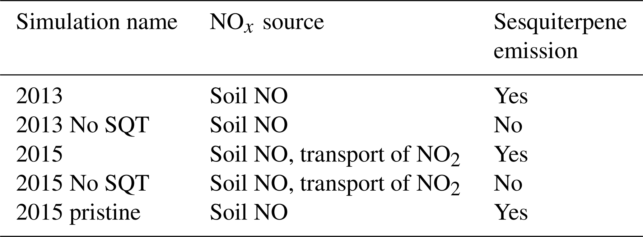
We test the hypothesis that sesquiterpene emissions have an important role in canopy-scale O₃ deposition fluxes via chemical removal inside the canopy by including simulations with and without sesquiterpene emissions. We also consider if transported NO₂ from biomass burning in 2015 could impact O₃, BVOC and NO_x exchange at the canopy top.

2.4 Canopy exchange calculations

To estimate a canopy exchange flux of NO_x and O₃ (E_x; $\mathrm{nmol}{\mathrm{m}}^{-\mathrm{2}}{\mathrm{s}}^{-\mathrm{1}}$) from the canopy to the atmosphere, we use the formula defined in Rummel et al. (2007), which specifically accounts for temporary storage of trace gases within the canopy:

$$\begin{array}{}\text{(19)}& \begin{array}{rl}{E}_x& ={\int }_{\mathrm{0}}^h{\text{Chem}}_{\text{net}}\left(z\right)\mathrm{d}z-{\int }_{\mathrm{0}}^h\text{Dep}\left(z\right)\mathrm{d}z\\ & +{\int }_{\mathrm{0}}^h\text{Emission}\left(z\right)\mathrm{d}z+{\displaystyle \frac{\mathrm{d}}{\mathrm{d}t}}{\int }_{\mathrm{0}}^h\left[x\right]\left(z\right)\mathrm{d}z\end{array}\end{array}$$

where x is either O₃ or NO_x and each term describes the integrated sum of chemistry, deposition, emission rates and storage across the vertical canopy levels z from soil level to canopy height h. Chem_net(z) refers to the net chemical production and loss rates at each height z. The storage term $\frac{\mathrm{d}}{\mathrm{d}t}{\int }_{\mathrm{0}}^h\left[x\right]\left(z\right)\mathrm{d}z$ represents any gas that is formed within the canopy or otherwise trapped within the canopy, that causes the in-canopy concentration to change. For example, soil-emitted NO does not immediately become an above-canopy flux, for a time it is trapped within the canopy and can be identified by an increase in within-canopy NO_x concentrations.

In the case of NO_x in 2015, it is useful to further separate the canopy exchange into the contributions from transported NO₂ and soil NO to calculate a canopy escape efficiency of soil NO_x. The contribution from upwind NO₂ transport into the canopy, E_{NOx_transp}, is estimated as the canopy exchange from a simulation of 2015 with no soil NO. This contribution is removed from simulations that contain both soil NO and transported NO₂ to give the soil NO_x escape efficiency.

$$\begin{array}{}\text{(20)}& {\text{Escape}}_{\text{NOx}}=E_{\text{NOx}}-E_{\text{NOx\_transp}}\end{array}$$

3 Results

3.1 Simulation evaluation

November 2013 at the ATTO site was a typical month in terms of temperature and wind velocity (Schmitt et al., 2023). November 2015 was atypical; El Niño conditions caused temperatures at ATTO to be 3 °C higher compared to 2013 and 1.5 °C higher across the Amazon compared to average (Jiménez-Muñoz et al., 2016). The 2015/16 El Niño drought reached maximum intensity in October 2015, with forest fires in November continuing to burn as though it was still the dry season (Ribeiro Neto et al., 2022; Silva Junior et al., 2019). During this period, the wind at ATTO predominantly originated from the Arc of Deforestation in the East (Fig. S11a), the location of enhanced fire activity (Silva Junior et al., 2019).

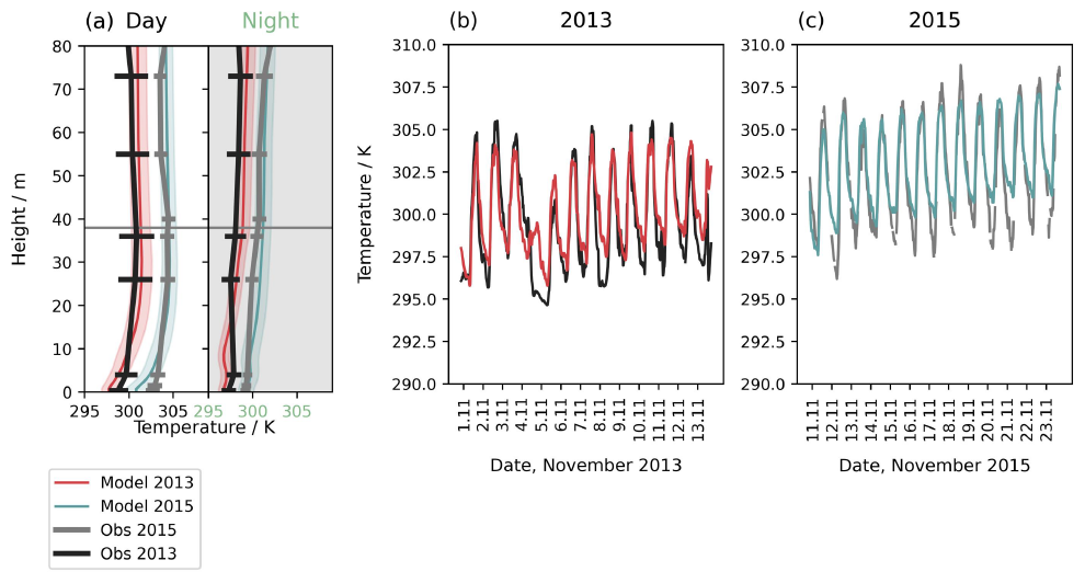
Figure 2 (a) Mean vertical profile of air temperature for day and night for simulations of November 2013 (red solid line), 2015 (teal solid line) and observations in 2013 (black solid line) and 2015 (grey solid line). Horizontal lines and shading show the daily mean standard deviation. (b) and (c) show the time series evaluation at 36 m for (b) 2013 and (c) 2015 simulation periods.

Measurements of atmospheric composition at ATTO during November 2015 showed increased OH reactivity, monoterpene emissions and oxidation product-to-isoprene ratios compared to previous years (Pfannerstill et al., 2018, 2021; Yáñez-Serrano et al., 2015, 2018). Daily mean O₃ concentrations in November 2015 were elevated compared to previous years, reaching up to 28 ppbv at 38 m, whereas 2013 concentrations varied between 4 and 16 ppbv at the canopy top, typical for the ATTO site (Fig. 11b).

We evaluate temperature and wind in our simulations and find the model reproduces temperatures in the 2013 and 2015 periods well (r²=0.80), albeit with a smaller diurnal range than observed and a stronger vertical gradient below the canopy (Fig. 2). Previous applications of the FORCAsT model also find the simulated diurnal variability is lower than observed (Wei at al., 2021). The model captures the difference between years and the day-to-day variability (Fig. 2b and c). The surface-level temperatures, which affect the soil NO emissions, reproduce night-time observations but underestimate the maximum temperatures in the daytime. The horizontal wind profile and hourly variability within the canopy is reproduced (Fig. S12). Above the canopy, however, the nighttime wind speed is underestimated on several nights, especially in 2013. Measurements show windspeeds above the canopy are frequently maintained around 2–4 m s⁻¹ overnight at 70 m, whereas friction velocity, which controls simulated wind speed, drops substantially, driving this underestimation (Fig. S12b).

Divergence between friction velocity and horizontal wind speed above the canopy has implications on vertical mixing within the model. Observed wind speeds are low in the canopy at night, but remain high above the canopy. This indicates decoupling between the canopy and above under stable, stratified nighttime conditions. Frequently in 2013 and on several nights in 2015, nights show high wind shear and sustained wind speeds above the canopy (Fig. S13). Richardson numbers in both periods are above 0.25 at night, which suggests turbulence is suppressed and intermittent (Fig. S14). However, the model likely overestimates the degree of turbulence suppression in 2013. The simulated flow has very low shear at night, meaning shear-driven mixing in the boundary layer is underestimated (Figs. S13a and S14c). This arises from the model reliance on friction velocity to constrain turbulent exchange, meaning intermittent turbulence is not captured when friction velocity is low. As a result, vertical mixing in the above-canopy space is overly weak on some nights in the simulations, with possible implications for the representation of exchange with the canopy.

Below the canopy, vertical turbulent exchange in our simulations shows strongly decreased vertical mixing at night, with stable air throughout the canopy especially between 01:00–05:00 LT (05:00–09:00 UTC) in both years. By midday, the canopy is well-mixed down to the lowest 20 %–30 %, which remains more separated from the air above (Fig. S15). Mixing below the canopy is enhanced in the 2015 period compared to the 2013 period during daytime on average across the simulation periods (Fig. S16). In observations, Pfannerstill et al. (2018) also found increased turbulent features during 2015, however we also note that missing observations of 2013 σ_w may affect our results. We find the meteorological performance of the model at this site to be comparable to simulations of the temperate forest, even when extending the simulation time considerably from previous 2 d studies (Wei et al., 2021).

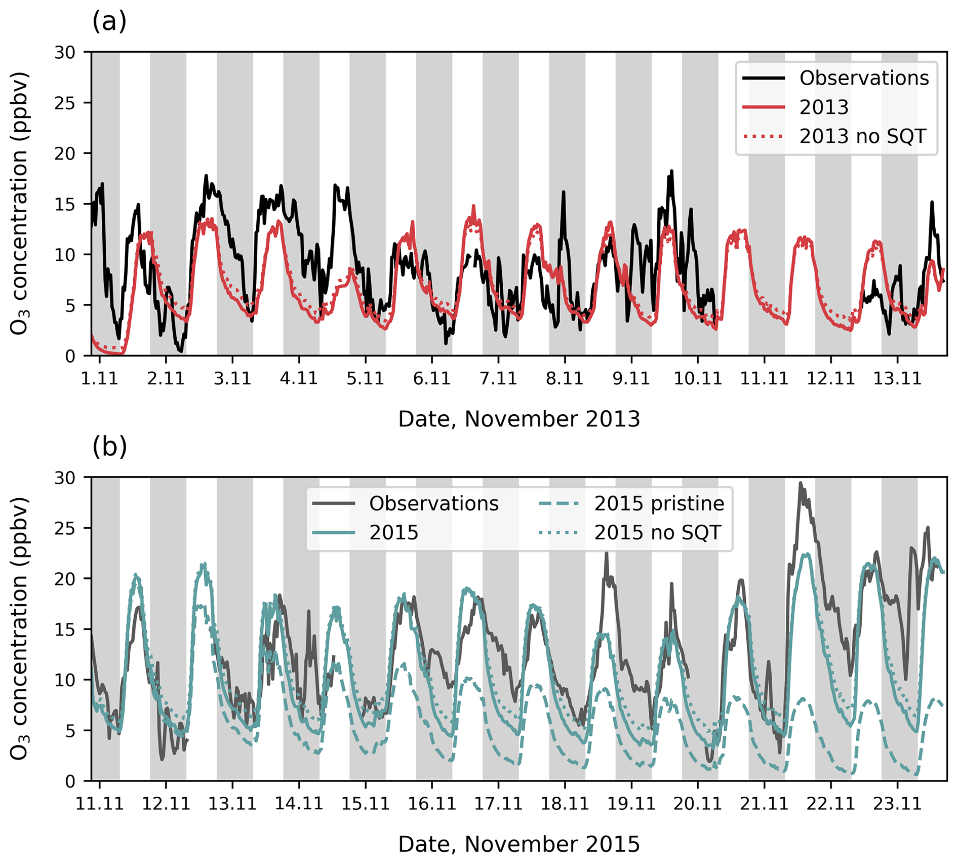
Figure 3 Above-canopy O₃ concentrations at 38 m from observations (solid black line) compared to simulations (coloured lines) for (a) November 2013 and (b) November 2015. Axis ticks are placed at midnight, and grey shading shows nighttime. In (a) simulations include O₃ concentrations with (red solid line) and without sesquiterpene emissions (red dotted line). In (b) simulations include O₃ concentrations when transport of NO₂ is included (teal solid line), without transported NO₂ (teal dashed line) and without sesquiterpene emissions (teal dotted line).

As a final evaluation of the model, we consider the partitioning of energy into latent and sensible heat fluxes above the canopy (Fig. S17). Average maximum hourly latent heat fluxes are 250 W m⁻² for the 2013 simulation period and 310 W m⁻² for the 2015 period, in good agreement with observations from the nearby LBA-k34 flux tower, which recorded hourly maxima of 250 and 300 W m⁻² for wet and dry season means, respectively (Gerken et al., 2018). Sensible heat fluxes are 80 and 100 W m⁻² in 2013 and 2015, respectively, compared to 110–150 W m⁻² in the nearby observations for wet and dry seasons. As a result of the lower magnitude and differences in the sensible heat flux diurnal cycle compared to observations, the Bowen ratio is higher in the morning and lower in the evening relative to the flux site values. However, the mean values of 0.4 in 2013 and 0.32 in 2015 (Fig. S17c) are close to observations (0.5) and represent an improvement over many land surface models (Restrepo-Coupe et al., 2021). These values suggest 2015 was not strongly water-limited in our simulations, with energy partitioning primarily responding to radiation. Observations of pristine tropical forests typically show seasonal cycles driven by radiation, with water stress rarely limiting (Restrepo-Coupe et al., 2021), making the model behaviour plausible, despite lacking directly comparable observations.

Figure 3a shows the model can reproduce the general magnitude and diurnal cycle of O₃ concentrations in the 2013 period. However, day-to-day variability is not well captured, especially the patterns in peak O₃ concentrations among different days. One of the vertical mixing components (σ_w) is not available for 2013, so any contribution to day-to-day variability that may occur from mixing cannot be fully represented. In November 2015, the magnitude of measured O₃ concentrations can only be reproduced when upwind transport of NO₂ from fires is included (Fig. 3b). Without transported NO₂, O₃ concentrations in the 2015 period are lower than 2013 concentrations despite higher temperatures, but when included, average O₃ concentrations over the 2015 simulation period are almost doubled. We find that inclusion of transported NO₂ captures the daily variability in peak O₃ concentrations on most days (Fig. 3b). This suggests that advected biomass burning air masses, resulting from higher fire activity in November 2015 compared to average (Ribeiro Neto et al., 2022; Silva Junior et al., 2019), are the main driver of higher O₃ concentrations at the site in 2015 rather than other meteorological differences such as higher temperature. Sensitivity tests in which sesquiterpene emissions are switched off are 1–2 ppbv higher at night, providing a better match to observations on average but not necessarily capturing the day-to-day variability better (Figs. 3 and 4a, b). Since we use a high O₃ reactivity to represent sesquiterpenes, the comparison of simulations with and without sesquiterpenes gives an uncertainty range on the effect of these emissions on O₃ concentration.

In both 2013 and 2015 simulation periods, the model performs worst overnight, often failing to capture nights in which O₃ is maintained at high concentrations, including in the lower canopy on three nights in 2015 (Fig. 3). High nighttime O₃, such as on 14 November 2015, are most likely related to missing turbulent features in our model. Nights with high O₃ concentrations above the canopy are often associated with high wind shear that is not reproduced by the model, suggesting turbulence within the boundary layer that brings O₃ to the canopy top (Fig. S13). Below the canopy, nighttime O₃ concentrations are reproduced on most nights in the model. The model captures the O₃ diurnal cycle more closely in the tropics compared to previously simulated temperate forests (Ashworth et al., 2015; Wei et al., 2021) due to the smaller influence from transported air masses at this site.

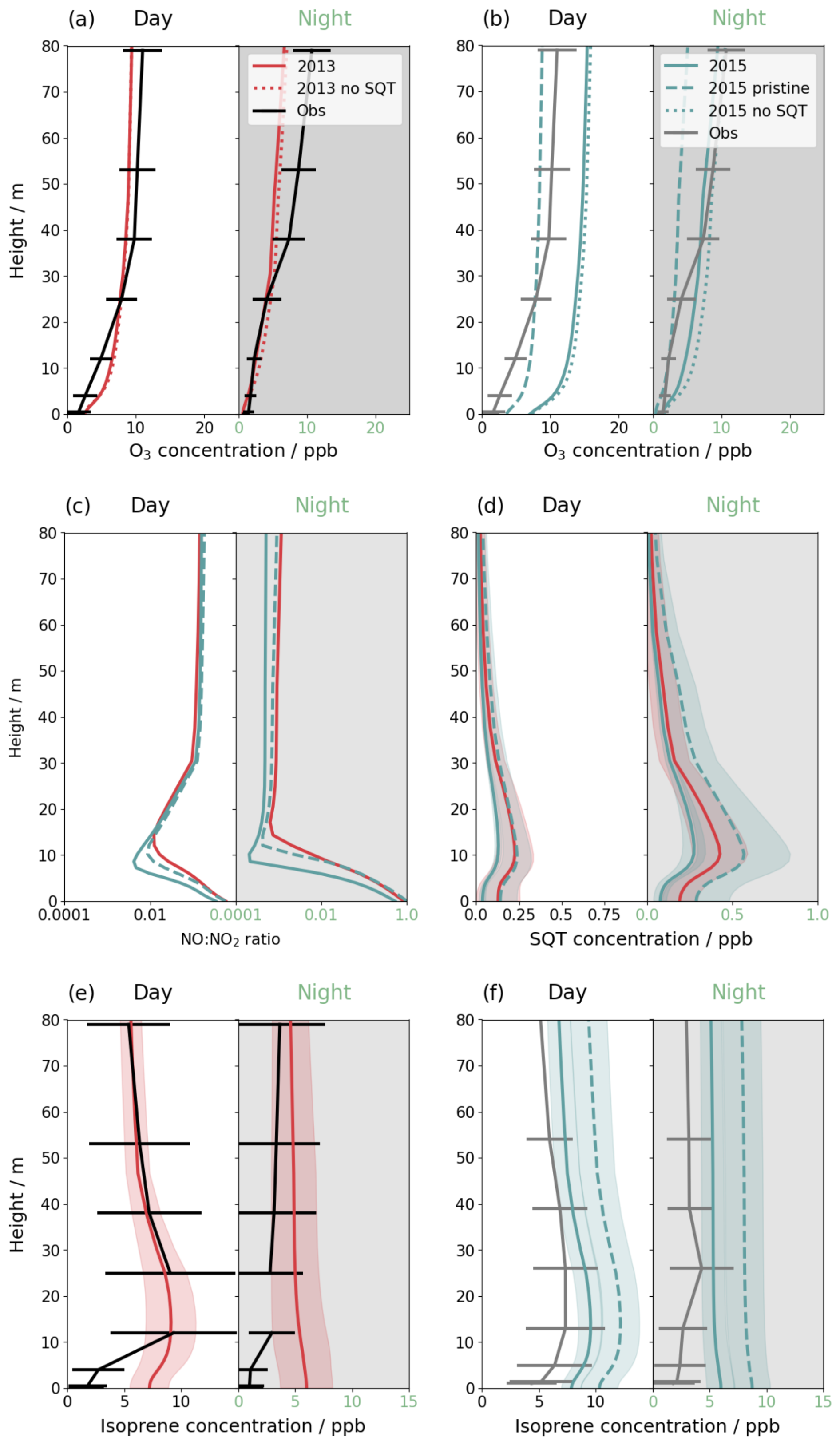
Figure 4 Mean vertical profiles for day and night in simulation periods of 2013 (red solid line), 2015, including transported NO₂ (teal solid line) and 2015 without transported NO₂ (teal dashed line) for (a) O₃ in 2013, (b) O₃ in 2015, (c) NO:NO₂ ratio, (d) sesquiterpene concentrations, (e) isoprene concentration in 2013 and (f) isoprene concentration, in 2015. Simulations are compared to observations (a) of O₃ in November 2013 (black solid line), (b) of O₃ in and November 2015 (grey solid line), (e) of isoprene in November 2012 (black solid line) and (f) of isoprene in October 2015 (grey solid line). Error bars and shading show one standard deviation of daily means. The grey horizontal line indicates the canopy height.

Figure 4a and b confirm that, whilst the daytime O₃ profiles are a good match to observations, nighttime profiles are underestimated, especially above the canopy. The step-change in O₃ gradient below the canopy in observations of the 2013 period suggests some decoupling between the canopy and above occurs, as also indicated by the sustained wind and low friction velocity above the canopy, described above (Fig. S12b and c). The lack of intermittent turbulence above the canopy in the simulations leads to underestimation of the above canopy O₃ profile, but decoupling results in a smaller bias below the canopy. The shape of the daytime vertical profile in the 2015 period is better captured than in the 2013 period; the observed 2013 vertical concentration gradient is steeper than 2015 but this is not replicated by the model.

Simulations of 2015 with transported NO₂, which produces additional O₃, consequently have a higher oxidative capacity. In pristine conditions, midday peak OH concentrations above the canopy are on average 1.3×10⁶ cm⁻³, decreasing to 0.4×10⁶ cm⁻³ within the canopy (not shown). The addition of transported NO₂ increases OH by 2× above the canopy, with diminishing differences between simulations below the canopy. Literature values from recent site measurements report 1×10⁶ cm⁻³ (Jeong et al., 2022), of similar magnitude to our simulations.

Transported NO₂ is also associated with a change in the NO:NO₂ ratio (Fig. 4c) in the lower canopy. In pristine conditions, the NO:NO₂ ratio is 0.5 and 1 at the soil surface in the day and night, respectively, decreasing to 0.35 (day) and 0.5 (night) when NO₂ transport is included in the 2015 simulation period. The elevated O₃ concentrations expedite the cycling of NO to NO₂, which removes NO in the dark lower canopy. By 10 m height within the canopy, NO concentrations are near zero in all simulations; NO is only re-formed closer to the canopy top where daytime photolysis is possible. Transported NO₂, of which very little reaches the soil level, does not strongly affect the NO:NO₂ ratio and the above-canopy ratio does not depend strongly on the simulation.

Even with the inclusion of transported NO₂, NO_x concentrations above the canopy remain below 1 ppbv (Fig. S18). Transported NO₂ can increase the above-canopy nighttime NO₂ concentrations from ∼300 pptv to up to 600 pptv (e.g., on 16 November 2015), increasing daytime NO as well. The values in pristine conditions compare well to observations at another Amazon site that measures pristine nighttime values of 350 pptv but find pollution enhancements of up to 1800 pptv (Cordova et al., 2004). Simulations show a distinct NO peak at sunrise as soil emissions are released from the canopy. These peaks show significant daily variability from 25 pptv to over 100 pptv, with daytime mean concentrations of 25 pptv without transported NO₂ and 50 pptv when NO₂ transport is included (Fig. S18c). The addition of transported NO₂ results in a less steep decay in NO from the midday peak. These values fit with observations recording 20–50 pptv above the Amazon forest canopy (Bakwin et al., 1990; Kuhn et al., 2010). Soil NO emissions therefore affect above-canopy NO_x concentrations significantly across all simulations.

Ground-level concentrations of NO depend strongly on O₃ concentrations, with even a few ppbv of O₃ rapidly removing emitted NO. Our simulations show very low nighttime O₃ concentrations (in agreement with observations), resulting in NO concentrations of 2–4 ppbv. This is consistent with observations from Rummel et al. (2002) who record lower NO concentrations of up to 2 ppbv but higher nighttime O₃ values. Conversely, ground-level daytime O₃ at the ATTO site is higher than measured by Rummel et al. (2002) and simulated daytime NO concentrations are below their measurements of 1.2 ppbv. Our daytime ground-level NO concentrations are closer to those of Bakwin et al. (1990) at 450 pptv.

High temperatures and PAR in the 2015 simulation increase BVOC emission compared to the 2013 simulation; isoprene emissions increase by 50 % and sesquiterpenes by 35 % (Fig. S19). However, the concentration profiles (Fig. 4d–f) are also related to background chemical composition. Simulations of the 2015 period in pristine conditions have higher BVOC concentrations compared to those with transported NO₂, as the lower oxidative capacity in pristine conditions leads to slower oxidation. With NO₂ transport included in 2015, isoprene concentrations are similar to the 2013 period concentrations, in both simulations and observations. The higher emissions in the 2015 period are balanced by increased oxidation. Concentrations of sesquiterpenes are lowest in 2015; the increased loss from the higher O₃ concentrations outweighs the increase in emissions (Fig. 4d). In all simulations, sesquiterpenes build up overnight within the canopy as vertical mixing declines and oxidation decreases, leading to higher concentrations at night compared to during the day in agreement with observations (Jardine et al., 2011).

Very low isoprene concentrations are recorded below the canopy (Fig. 4e and f) that are consistently overestimated by the model. Some studies find isoprene loss fluxes to tropical soils (e.g., Pugliese et al., 2023) that are not explored in this study.

3.2 O₃ losses in the canopy

Figure 5a shows the mean total canopy flux of O₃ over the simulation period, divided into net chemical loss and deposition (as in Eq. 19). The O₃ mostly originates from above the canopy, meaning the canopy is a net O₃ sink. The total flux in 2013 is −2.4 $\mathrm{nmol}{\mathrm{m}}^{-\mathrm{2}}{\mathrm{s}}^{-\mathrm{1}}$ compared to −3.9 $\mathrm{nmol}{\mathrm{m}}^{-\mathrm{2}}{\mathrm{s}}^{-\mathrm{1}}$ in 2015, whereas the total flux in the 2013 simulation period and an idealised 2015 period with no transported NO₂ are very similar (i.e., the main difference between 2013 and 2015 simulation periods is related to effects of transported NO_x). Simulations without sesquiterpene emissions have very little effect on the total flux.

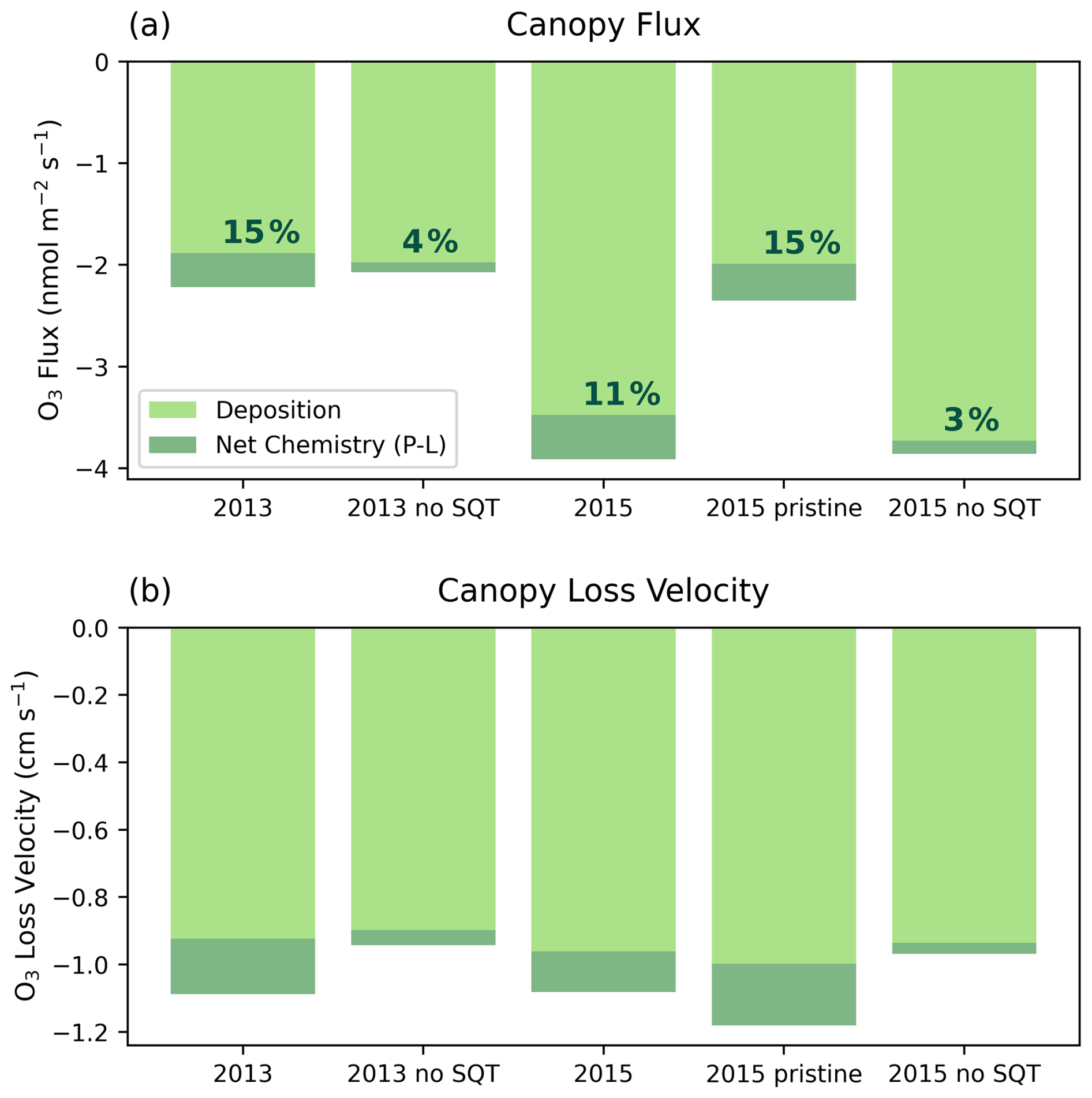
Figure 5 (a) The mean flux of O₃ in $\mathrm{nmol}{\mathrm{m}}^{-\mathrm{2}}{\mathrm{s}}^{-\mathrm{1}}$ and (b) the canopy-scale deposition velocity in cm s⁻¹ divided into deposition (light green) and net chemistry (dark green). Text given in (a) indicates the percentage of the total flux that is chemical destruction.

Considering the breakdown of the flux into chemical and depositional components, we find that deposition accounts for the majority of O₃ losses in all simulations. The fraction of total loss that is due to chemistry is slightly higher in simulations without transported NO₂ at 15 % compared to 11 % when transport of NO₂ is included (Fig. 5a). Without sesquiterpenes, the fraction of O₃ loss due to chemistry reduces to 3 %–4 %, however the decrease in chemical flux is partly compensated by an increase in deposition flux. This may suggest that sesquiterpenes can reduce the deposition flux to vegetation through reducing the O₃ available for deposition and thus have the potential to reduce O₃ damage to vegetation. On the other hand, since the difference in the total flux is small, it indicates that the total O₃ in-canopy loss is somewhat resistant to uncertainties in sesquiterpene emissions and chemistry.

Figure 5b shows the equivalent losses presented as a canopy-scale deposition velocity. Variability in the canopy deposition velocity is much smaller than in the total O₃ flux, with a range of −0.9 to −1.2 cm s⁻¹ among the simulations, implying that most of the difference in flux is related to differences in the O₃ concentrations. The major differences are (1) a small variability of −0.04 cm s⁻¹ in deposition velocity between simulations, (2) an increase in chemical loss velocity in the absence of transported NO₂ in 2015, and (3) a decrease in chemical loss velocity without sesquiterpene chemistry.

Diurnal patterns of individual flux terms (chemistry, deposition and storage) show the same features identified by Rummel et al. (2007) such as an increase in storage in the morning as vertical transport brings O₃ into the canopy from above (Fig. S20). Observed fluxes are also similar in magnitude to our simulations but cannot be directly compared as they depend strongly on O₃ concentration. Observations of canopy deposition velocities are larger in the wet season compared to the dry season, attributed to humidity-driven stomatal limitation in the dry season. Our simulated deposition velocities are within the range of wet season observations but are higher than dry season averages of ∼0.5 cm s⁻¹ (Rummel et al., 2007). Our simulations show high relative humidity (Fig. S21) and daytime temperatures (Fig. 2) close to the simulation optimum parameter for stomatal conductance (301 K), suggesting little stomatal limitation and therefore “wet season” behaviour. This is consistent with evaluation of the energy balance and Bowen ratio described above (Sect. 3.1, Fig. S17). Day-to-day variability in deposition velocity in the simulations follows variability in temperature and PAR (Fig. S22). The 2013 period exhibits lower average PAR and greater daily variability (including a cool, cloudy day on the 4th), resulting in lower average stomatal conductance than the 2015 period (Fig. S23). However, differences in deposition velocity between simulations are likely also related to changes in O₃ distribution within the canopy.

In the remainder of this section, we consider the chemistry within the canopy, first using Fig. 6 to explore differences in chemical loss velocity between years and simulations. The vertical profiles of net chemistry in Fig. 6 elucidate the role of BVOCs and soil NO in driving O₃ losses within the canopy. In addition to removal by BVOCs in the canopy, soil NO is responsible for O₃ removal at the lowest model level, which compares to the reports from another Amazonian site (Gut et al., 2002). The chemical loss velocity profiles for simulations without sesquiterpene emissions show that loss by reaction with soil NO is of similar magnitude to O₃ removal by other BVOCs and the in-canopy profiles are very similar between years, which suggests sesquiterpenes are responsible for the differences in net chemistry. We find that consideration of both sesquiterpene emissions and O₃ concentrations are required to explain the canopy average loss velocity; there is a robust but non-linear relationship between canopy O₃ chemical loss and the ratio of sesquiterpene emissions to O₃ concentrations at 30 min resolution (Fig. S24). A decrease in chemical loss in 2015 in polluted conditions can be explained by an increase in O₃ concentrations, and faster losses in 2015 in pristine conditions can be explained by an increase in sesquiterpene emissions compared to 2013, on account of higher PAR and temperature. Differences between simulations are greatest at 20–25 m where the leaf area density (and associated BVOC emissions) is highest, whereas at the soil surface, chemical loss frequencies are similar.

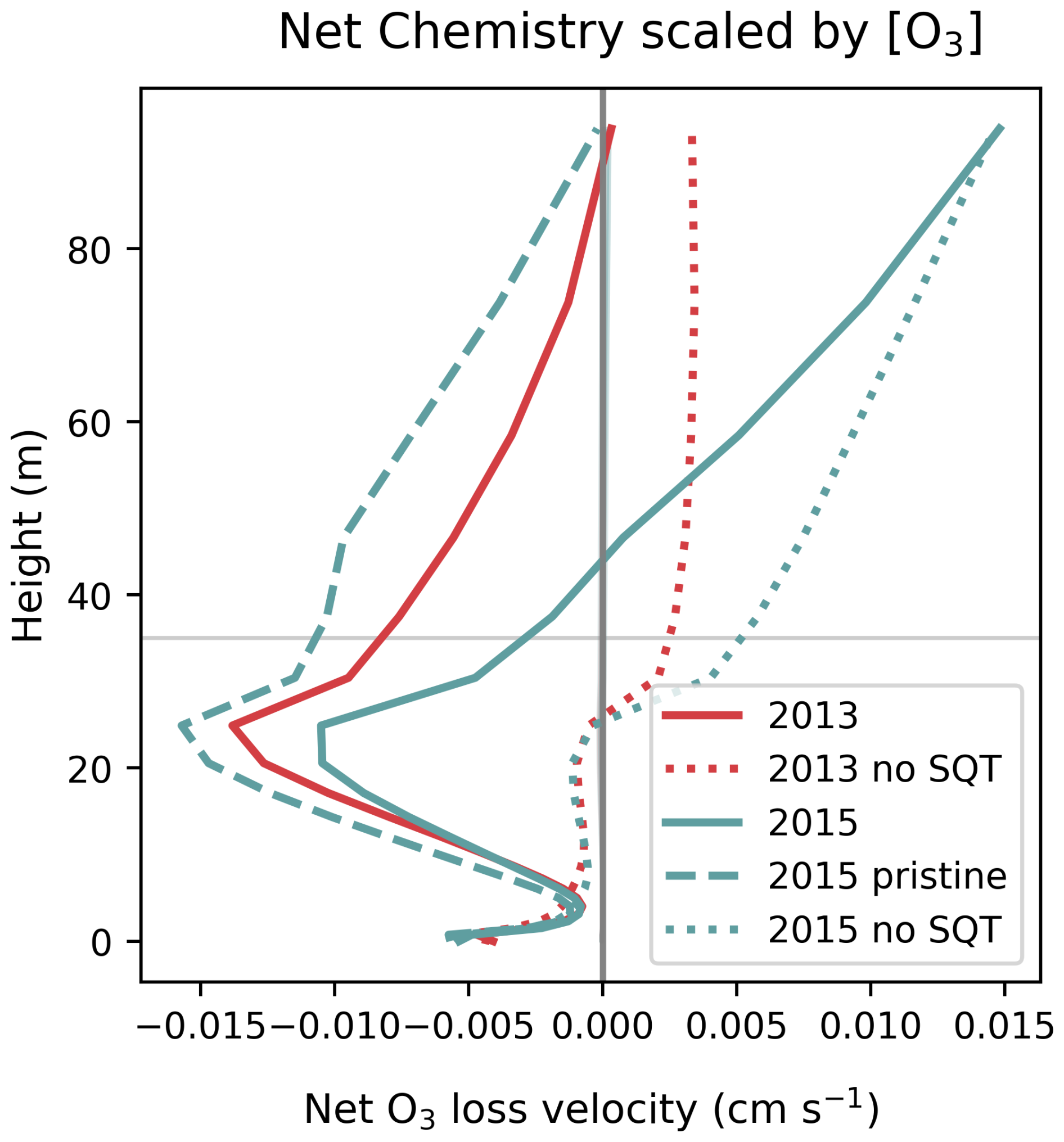
Figure 6 Vertical profiles of simulated net O₃ chemistry (production − loss) divided by O₃ concentration to give the loss velocity per molecule for simulation periods in 2013 (red lines) and 2015 (teal lines). Sensitivity tests show simulations without sesquiterpenes (dotted lines) and 2015 without transport of NO₂ (teal dashed line). The horizontal line indicates the canopy top height.

Figure 7 shows the diurnal cycle of chemical production and loss occurring at 25 m, to demonstrate how chemistry varies over the day at the bulk canopy height (Fig. 1). Considering the individual reactions involved in O₃ chemical loss (Fig. 7, green shading), sesquiterpene ozonolysis dominates at all times of day and is entirely responsible for nighttime chemistry at this height. Other BVOCs contribute to O₃ destruction during the afternoon and 2015 has a more substantial morning contribution from radical losses. Considering the whole canopy, over the diurnal cycle, chemistry is most important during the night, where it can account for 40 % the total O₃ losses (Fig. S20). During the day, its contribution to the canopy O₃ flux diminishes to 5 %, which is in response to an 8-fold increase in deposition flux as stomatal pathways become available, rather than a significant change in chemistry.

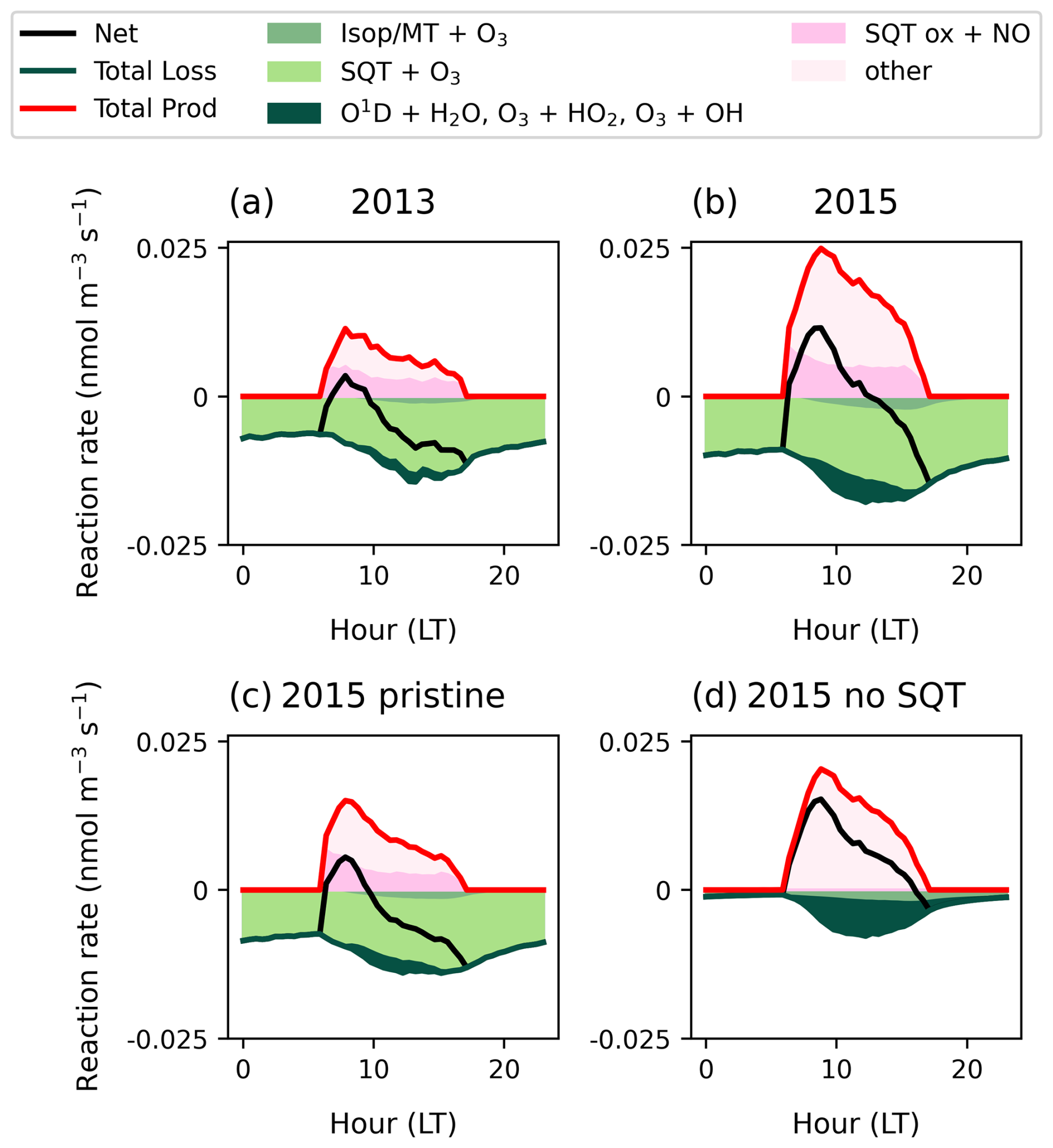
Figure 7 Mean diurnal cycles at 25 m of chemical reactions for O₃ loss (green solid line), production (red solid line) and net chemistry (black solid line). Individual reactions are shaded showing sesquiterpene ozonolysis (light green shading), isoprene / monoterpenes + O₃ (medium green shading) and inorganic O₃ loss (dark green shading). For O₃ production reactions, β-carophyllene oxidation products is the largest uncertainty (dark pink shading).

The diurnal cycle reveals that even at 25 m, simulations switch to net O₃ production after sunrise and the breakdown of the nighttime boundary layer (approx. 06:00 LT) (Fig. 7, black solid line). O₃ production (Fig. 7, red solid line) is driven by a large number of oxidation products in the presence of NO; the three largest contributors are isoprene oxidation products, HO₂ and sesquiterpene oxidation products. As the largest uncertainty, the contribution from sesquiterpene oxidation products is shown in dark pink shading; it counteracts a substantial portion of daytime losses due to sesquiterpenes at this height. Production is smallest in 2013 and enhanced in the presence of transported NO_x (Fig. 7b) such that net production of O₃ continues until 13:00 LT on average compared to until 10:00 LT in pristine conditions (Fig. 7c). Without sesquiterpenes, net O₃ production occurs throughout daylight hours (Fig. 7d). The significant diurnal variability in O₃ production suggests that canopy escape efficiencies of precursors (especially NO_x and sesquiterpenes) should be investigated across the diurnal cycle.

In the mean vertical profile (Fig. 6), the transition to net O₃ production occurs at different heights among simulations. Addition of transported NO₂ triggers net production at 40 m whereas in pristine conditions, profiles in the 2013 and 2015 simulation periods both show net loss of O₃ up to 100 m. Without sesquiterpene emissions, net O₃ production begins immediately above the main canopy density at 25 m, where light is not strongly attenuated and can initiate photolysis (Fig. 1). Simulations with and without sesquiterpene emissions converge at around 100 m, indicating the point at which sesquiterpenes are fully oxidized. A significant portion of O₃ losses by sesquiterpenes occur above the canopy, implying that accurate quantification of sesquiterpene escape efficiencies is important for above-canopy chemistry.

3.3 The role of BVOCs in canopy chemistry

BVOC escape efficiency is controlled by their oxidation rate with respect to OH, O₃ and NO₃, such that the faster a species can be removed (dependent on reaction rate and oxidant concentration), the lower the escape efficiency. For the oxidant concentrations at this site, escape efficiencies of primary emitted BVOCs increase in the order; sesquiterpenes ≪ limonene < α-pinene < isoprene. Furthermore, depending on transport and oxidant concentration between simulations, BVOC escape efficiencies vary among simulations.

The escape efficiency of sesquiterpenes ranges from 45 %–55 % between simulations. The highest escape efficiency of 55 % occurs in 2015 pristine conditions. When transport of NO₂ is included, this decreases to 48 % as a result of higher O₃ concentrations. Both simulations of the 2015 period have a higher escape efficiency than the 45 % in 2013. The MEGAN 2.0 BVOC emissions model includes an escape efficiency to account for BVOC losses within the canopy, based on chemical lifetime, u_∗ and canopy depth (Guenther et al., 2006). This parameterisation results in canopy escape efficiencies from 10 % (in the presence of high O₃) to 60 %. Our results, in relatively low O₃ conditions compared to global averages, fit realistically within this wide range. We find a significant correlation exists between daily mean escape efficiency and u_∗ (r²=0.69, p≪0.05; Fig. S25). This indicates that, for single-layer canopy models seeking a simple parameterisation, the current equation in MEGAN 2.0 is functional.

Isoprene and α-pinene escape efficiencies are 95 % both with and without transported NO₂, and in both 2013 and 2015 simulation periods. This is despite different emission magnitudes of isoprene of 4.7 and 7.3 $\mathrm{mg}{\mathrm{m}}^{-\mathrm{2}}{\mathrm{s}}^{-\mathrm{1}}$ due to varying meteorological conditions (Fig. S19). The isoprene escape efficiency of 95 % with little variability is consistent with the parameterisation from MEGAN 2.0 (Guenther et al., 2006).

Conversely, limonene escape efficiency is slightly more sensitive to the environmental conditions, with escape efficiencies of 88 % in pristine conditions in 2015, dropping to 84 % with transported NO₂ and in 2013. These temperature-dependent pool emissions continue overnight when vertical mixing is slow, which allows more time for chemistry to act. This allows for greater differences in escape efficiencies between simulations due to chemical environments that are overcome during the day when vertical mixing is highly efficient and canopy residence times are short.

3.4 NO_x exchange with the canopy

3.4.1 Soil NO_x escape efficiency

Figure 8a shows the NO_x budget terms below the canopy and the overall escape efficiency of soil NO_x. The soil NO_x escape efficiency is different than the canopy NO_x flux (described in the next section) in that it excludes the contribution from upwind transported NO₂ into the canopy. To exclude this, we estimate the contribution from transported NO₂ entering the canopy using a simulation with no soil NO source and subtract this from the simulation of 2015 with transported NO₂ (as described in Sect. 2.4; Eq. 20). The motivation for isolating only the soil NO that leaves the canopy is to inform how soil NO emission should be represented by a single-layer canopy model. The comparison between 2015 and pristine 2015 reveals changes in soil NO emission resulting from a change in chemical environment (e.g., the NO_x production and loss terms depend on the background environment).

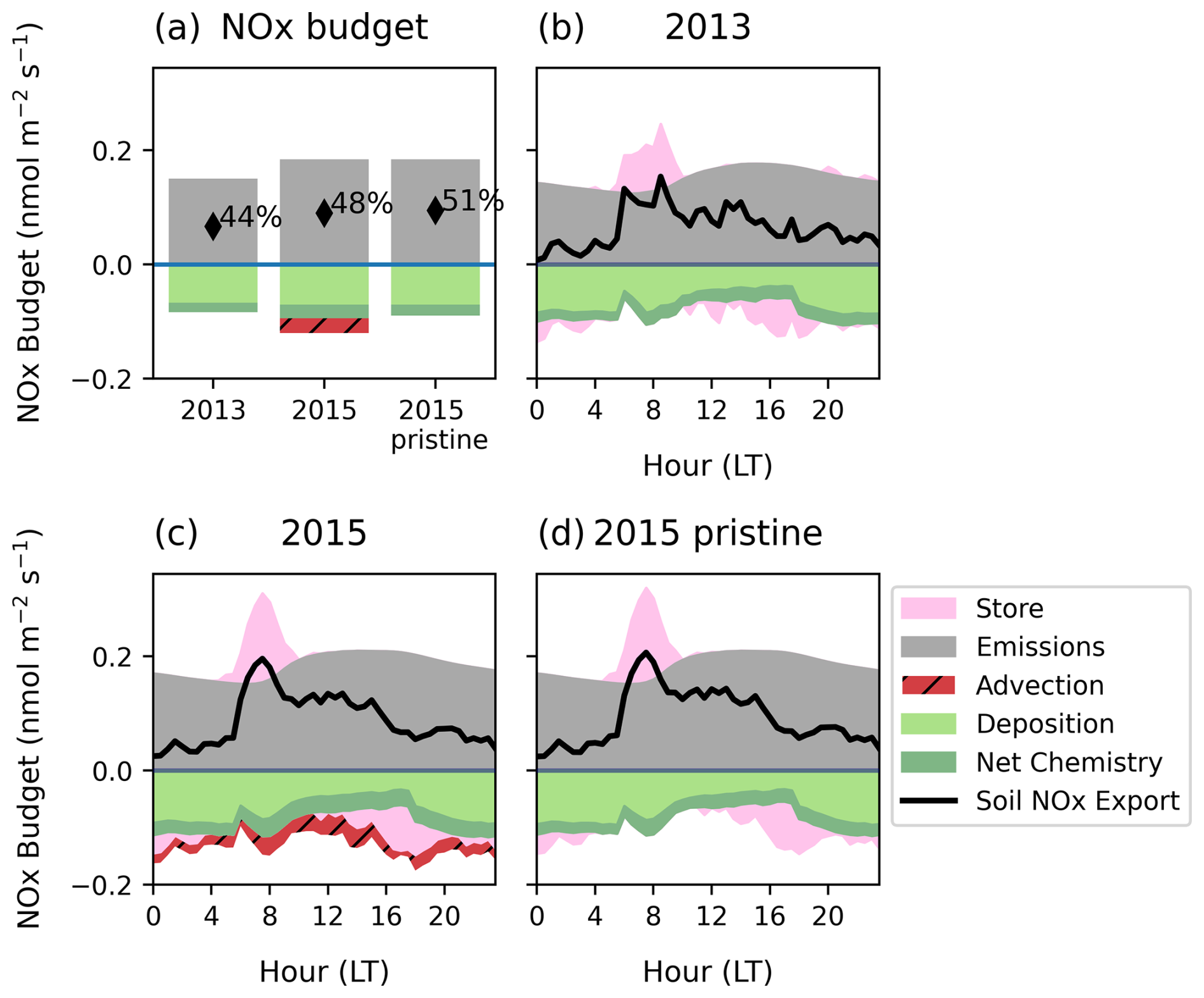
Figure 8 Mean diurnal NO_x budget at 35 m of soil NO emissions (grey shading), transfer of upwind transported NO₂ into the canopy (red shading), net chemical change (dark green shading), deposition (light green shading) and storage (pink shading) within the canopy for (a) the daily mean and (b, c) the mean diurnal cycle in individual simulations. (a) 2013, (b) 2015 simulation periods including transported NO₂ and (c) 2015 without transported NO₂. In (a), the text gives the escape efficiency. In (b) and (c) The sum of all terms except upwind transported NO₂ (black solid line) is the soil NO escape flux.

We find the 2013 escape efficiency of 44 % is lower than the 2015 period simulations, given the consistent deposition of 0.7 $\mathrm{nmol}{\mathrm{m}}^{-\mathrm{2}}{\mathrm{s}}^{-\mathrm{1}}$ across simulations despite lower emissions in the 2013 period. Comparing 2015 with and without transported NO₂ suggests the change in chemical environment due to upwind NO₂ transport has a relatively smaller effect on soil NO_x escape (48 % vs. 51 %) and therefore escape efficiency is more dependent on meteorological changes.

The diurnal cycle of soil NO_x escape at the top of the canopy shows considerable variability over the day, displaying a pronounced cycle that is largely unrelated to diurnal variability in soil NO emissions (Fig. 8b–d). Daylight hours have the highest escape efficiency, whereas NO_x release overnight is suppressed by in-canopy storage and enhanced deposition fluxes.

We first consider the role of storage in the diurnal pattern, which refers to NO_x that becomes trapped in the canopy space due to slow vertical mixing. Our simulations find the greatest transfer of stored NO_x from the canopy occurs at sunrise when stable separation between the canopy and above breaks down and photochemistry is initiated (Fig. 8, pink shading). This is very pronounced in 2015 when the escape from the canopy is greater than the instantaneous soil emission rate. This indicates strong separation between the below and above-canopy environment overnight that allows NO_x to build up.

NO emitted from the soil is rapidly oxidized to NO₂ when O₃ is present, but during the night, NO accumulates near the ground. At night, there is a significant flux to the soil and lower canopy surfaces (Fig. S26). As stomata are closed, this is likely non-stomatal deposition to the soil and cuticles that is high due to build-up of NO₂ in the lower canopy originating from the soil in low turbulence. With the onset of turbulent mixing under daylight, O₃ oxidises NO to NO₂, which is transported upwards but partially taken up by deposition to vegetation (Breuninger et al., 2013; Chaparro-Suarez et al., 2011; Gut et al., 2002). The greatest daytime deposition flux therefore also occurs at the onset of mixing as NO_x at the surface is brought to heights with greater leaf area (Fig. S26). However, the daytime deposition flux is lower than nighttime on average due to lower daytime concentrations.

Comparing across simulations, we find the escape efficiency in 2013 is lower at all times of day, with a smaller day-night contrast compared to the 2015 period (Fig. 8b). Over the course of the day, the escape efficiency varies from 25 %–100 % in 2013 and 30 %–130 % in 2015. Escape efficiencies over 100 % occur when release of stored NO_x in addition to emitted NO_x results in canopy fluxes greater than the instantaneous emissions. On the other hand, transport of upwind NO₂ in 2015 does not change the mean diurnal pattern significantly (cf. Fig. 8c and d); the morning storage release is slightly reduced, likely due to a reduced concentration gradient when NO₂ transport occurs.

Figure 9 demonstrates that vertical mixing can largely account for diurnal, daily and between-simulation variability in soil NO_x escape efficiency. There is a correlation between the eddy diffusivity coefficient K and NO_x escape efficiency (r²=0.50) across all simulations at a 30 min time resolution, suggesting half of the variability can be explained by vertical turbulence; longer canopy residence times increase the opportunity for deposition and other chemical losses in addition to in-canopy storage. Most of the variability is diurnal, although differences across days are also explained by the degree of mixing (Fig. S27). Among simulations, the reduced escape efficiency in the 2013 period relative to 2015 can be related to the slower vertical mixing, whereas the addition of transported NO₂ in 2015 causes an increase in net chemical removal that is unrelated to mixing parameterisations. The morning spike in NO_x escape is proportionally greater than the morning increase in K (Fig. S27) but is the main driver of O₃ production above-canopy in pristine conditions (Fig. 7). The concentrated release of NO at sunrise facilitates greater O₃ production than if the same emissions were distributed across the day and is therefore important for capturing O₃ chemistry in pristine conditions.

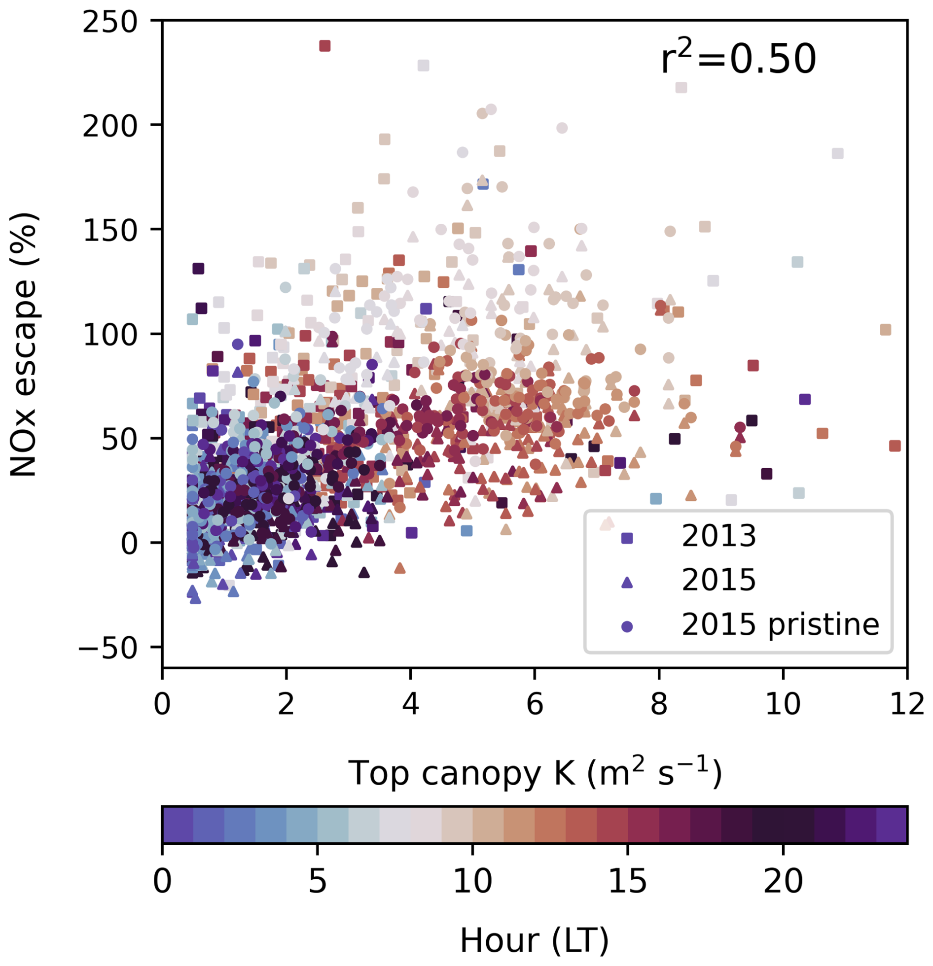
Figure 9 The turbulent exchange parameter K compared to NO_x escape efficiency in simulation periods of 2013 (square markers), 2015 including transported NO₂ (triangle markers) and 2015 without transported NO₂ (circle markers) in half hourly values. Shading indicated the hour in local time.

NO_x escape efficiencies are currently poorly constrained by observations. Comparison of single-layer parameterisations by Yienger and Levy (1995) to multilayer canopy calculations by Ganzeveld et al. (2002b) find tropical forest escape efficiencies are highly sensitive to in-canopy NO_x processes due to the role of chemistry and turbulence within the canopy. While single-layer estimates of 20 % likely overestimate the role of deposition, the multilayer average from Ganzeveld et al. (2002b) of 40 % is closer to our findings. We suggest that turbulence above the canopy is a good indicator of variability at this site without needing to resolve the full canopy structure and that resolution of the diurnal cycle in NO_x escape is most important for representing the majority of the variability in escape efficiency.

3.4.2 The fate of upwind transported NO_x within the canopy

Here, we consider how transported NO₂ above the canopy in the 2015 period affects the total canopy NO_x flux. When NO_x concentrations above the canopy are high, as can happen when NO₂ is transported, the canopy can become a net sink. This bi-directional exchange means the canopy flux can switch from positive to negative in polluted conditions.

Figure 10a highlights the first 6 d of the simulation to show that even with transport of NO₂, the canopy largely remains a NO_x source. This is likely because NO_x concentrations at the canopy top are not significantly enhanced in our simulations (Fig. S18). Exceptions occur when NO₂ transport occurs during the night; the transfer into the canopy at individual moments are greater than the soil NO escape, making the canopy a NO_x sink (also see Fig. S27b). This implies the canopy must remain a substantial depositional sink overnight.

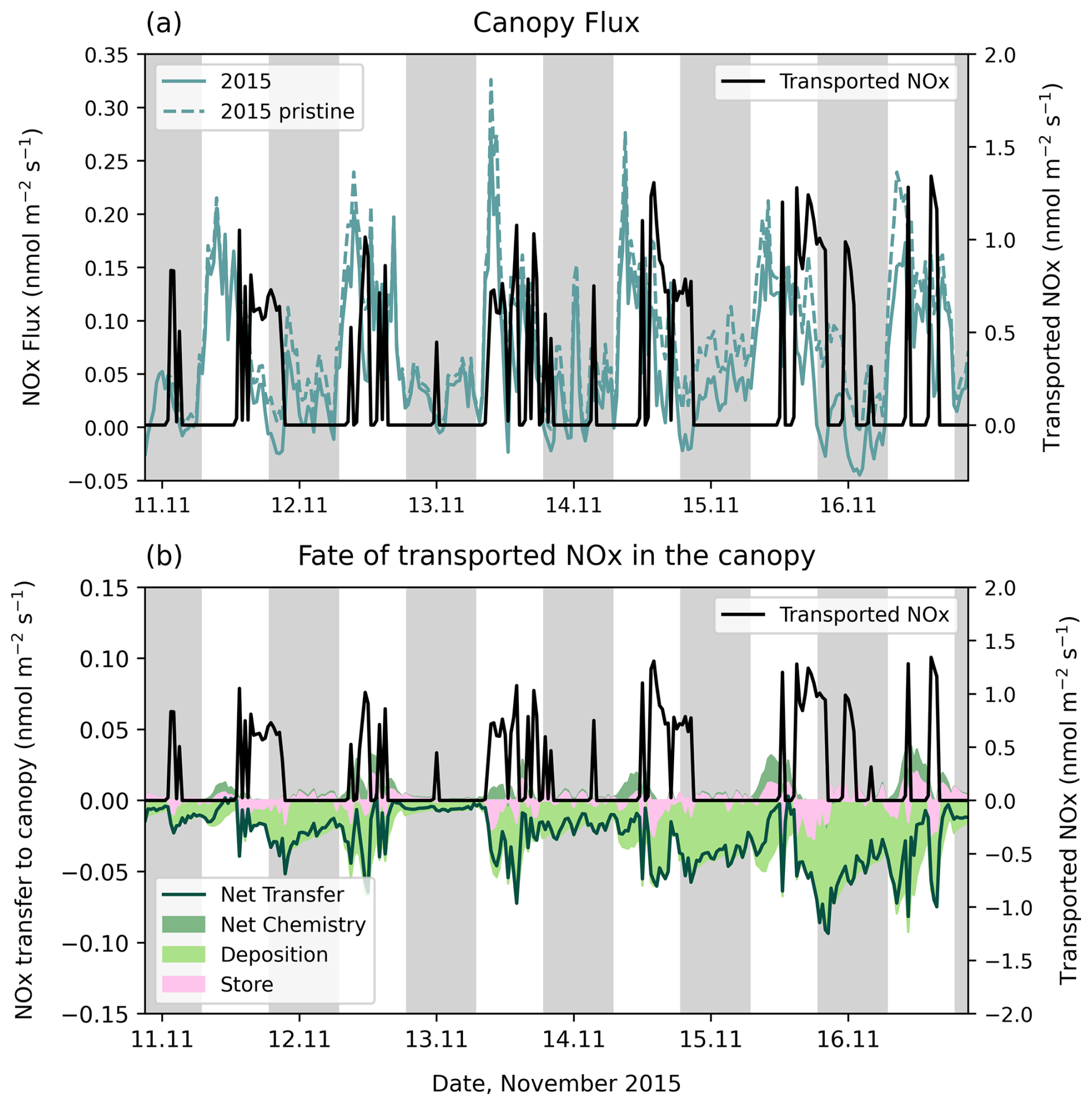
Figure 10 (a) NO_x transported from upwind above the canopy (black solid line) compared to the canopy-scale NO_x flux in 2015 for simulations with transported NO₂ (teal solid line) and with pristine conditions (teal dashed line). (b) NO_x transported from upwind above the canopy (black solid line) compared to transported NO_x entering the canopy (green solid line), divided into deposition (light green shading), net chemistry (dark green shading) and storage (pink shading). Tick marks on the x axis are placed at midnight.

Figure 10b identifies the fate of transported NO_x within the canopy to understand the source/sink behaviour. The instantaneous response to transported NO_x within the canopy is an increase in canopy storage and deposition. After the NO₂ transport ends, there is often a reversal of storage (i.e., a release of NO_x), although enhanced deposition continues. This is especially clear in the daytime of the 16th. During the day, NO₂ transport often results in an almost instant transfer to the canopy, such that the net transfer follows the same pattern as spikes in upwind transport. This is due to efficient mixing into the canopy during the day. During the night, upwind NO₂ transport is not immediately transferred into the canopy, for example overnight transport events on the 13th and 14th do not show up as spikes in net canopy transfer. Instead, deposition is often spread throughout the night, especially if there has been significant transport of NO₂ to the site in the early evening (e.g., night of 15th and 16th). This is in response to NO₂ that was transferred into the canopy during the day and remains trapped due to nighttime stagnation of vertical mixing. In this way, the canopy response to NO₂ transport lasts longer than the actual transport event above the canopy and depends on the time of day. The daytime transfer is often too small relative to the soil flux to cause net loss of NO_x to the canopy. During the night, however, sustained deposition of NO_x trapped within the canopy transforms the top of canopy flux to a net sink.

Most single-layer canopy deposition schemes do not account for continued deposition of NO_x stored within the canopy overnight. The resistance term includes an aerodynamic resistance that is lower when vertical turbulence is higher, describing enhanced transport into the canopy. However, a single-layer canopy cannot account for canopy storage, missing possible enhanced deposition of NO₂ during stagnant conditions overnight and may therefore underestimate NO_x losses to the canopy.

4 Discussion

We demonstrate that a column model at the ATTO site in the remote Amazon successfully captures the greater meteorological and concentration gradients characteristic of deep tropical canopies, expanding previous applications in more well-mixed temperate forest (Ashworth et al., 2015; Wei et al., 2021). Notably, the model successfully simulates a 2-week period whereas previous studies were limited to two days.

The model reveals the critical role of transported precursors from biomass burning in the tropics. The flux of O₃ into the canopy is highest in 2015, attributed to O₃ production above the canopy from transported NO₂ from the Arc of Deforestation. The higher O₃ concentrations lead to greater sesquiterpene ozonolysis, reducing the sesquiterpene escape efficiency (Sect. 3.3) whilst also decreasing the chemical loss velocity of O₃ (Fig. 5b). Because of the higher flux of freshly-formed O₃ into the canopy, absolute deposition and chemical losses increase (Fig. 5a). Biomass burning therefore increases stomatal O₃ flux, leading to a heightened risk of O₃ damage to the forest (e.g., Cheesman et al., 2024). We note that our representation of biomass burning by transport of upwind NO₂ is a substantial simplification; biomass burning is guaranteed to bring other trace gases not included in this simulation, which may impact background composition. Equally, wind arriving from the direction of the Arc of Deforestation has not necessarily passed through a biomass burning plume. Nonetheless, good representation of day-to-day variability in O₃ concentrations suggests this is a reasonable approximation (Fig. 3b).

Meteorological differences between simulation periods in 2013 and 2015 as a result of El Niño conditions, including higher temperatures and PAR in 2015, enhance BVOC emissions but produce only a small increase in canopy-scale O₃ deposition velocities (Fig. 5b). The sustained deposition velocities in the 2015 simulation suggest no significant stomatal limitation despite the extreme weather (Fig. 5b). Deposition schemes are highly parameterised and remain a substantial uncertainty in canopy modelling, and this study did not explore the leaf- or soil-level parameterisations in detail. As the majority of simulated O₃ and NO_x canopy losses occur via this pathway, greater focus is needed on accurately representing deposition within the canopy and its response to changing meteorological conditions. Whilst stomata play a crucial role, non-stomatal deposition on plant surfaces also have an influence (Sun et al., 2016), but these are often represented, including here, by simple parameterisations in models. Previous studies have identified non-stomatal deposition to wet leaf surfaces to be a potentially relevant removal process in the tropics, an aspect not considered in this study (Yáñez-Serrano et al., 2018). The effect of canopy wetness on deposition magnitude and escape efficiencies may therefore be important for soluble BVOCs and NO_x, and greater understanding of this process would enable improved parameterisations. Our simulations estimate sustained NO₂ deposition occurring overnight via non-stomatal pathways, leading to net canopy deposition when NO₂ is transported to the site (Fig. 10). Greater understanding of the partitioning between stomatal, cuticular and soil deposition is required to evaluate these conclusions.

Vertical turbulent mixing is a major contributor to variability in soil NO_x escape efficiency (Fig. 9) and, to a lesser degree, in the escape efficiency of pool BVOCs and transfer of upwind NO₂ into the canopy; increased residence time within the canopy as a result of reduced mixing increases opportunities for chemical loss and deposition, decreasing escape efficiencies. Qualitatively, vertical mixing profiles are comparable to other measurements at Amazon sites (e.g., Freire et al., 2017; Santana et al., 2018) although representation of downdrafts and large-scale canopy sweeps (Bardakov et al., 2022; Unfer et al., 2025) are not possible with our parameterisation but can dominate the transport process at this site (Cava et al., 2022). We find intermittent turbulence is likely underestimated in our simulations at night. For a more explicit representation of vertical mixing processes, large eddy simulations (LES) that include a canopy should be explored (e.g., Pedruzo-Bagazgoitia et al., 2023).

Our simulations repeatedly highlight sesquiterpenes as dominant species in O₃ chemical removal within and above the canopy (Fig. 7). Nonetheless, further measurements of sesquiterpene species and reactivity are needed to accurately quantify the impact on O₃ concentrations. Sesquiterpene measurements are not currently available at the ATTO site, such that the emission factors used here could be better constrained if measurements become available. Similarly, monoterpene emissions can include highly reactive species that have not been accurately characterised and our emission factors are estimated from observed concentration profiles rather than emission rate observations. We use the reactivity of β-caryophyllene to represent sesquiterpenes in our simulations, a species known for its high reactivity with O₃. This should be considered an upper limit on sesquiterpene contribution to reactivity, and therefore a lower limit on escape efficiency. Although β-caryophyllene is often a dominant species in measurements, farnesene, cadinenes, and muurolenes are frequently found to also be significant (Isaacman-VanWertz et al., 2024). A greater understanding of sesquiterpene emissions composition, and reactivity of other sesquiterpene classes would reduce uncertainty. Measuring the concentration of such highly reactive compounds in the atmosphere is severely hampered by their rapid decomposition; measurements must be taken close to the source. Our simulations also find that O₃ reactivity with sesquiterpenes can continue above 100 m (Fig. 6), which suggests sesquiterpene concentration measurements may be possible above the canopy, especially in pristine conditions, which could help to constrain the model further.

In addition to the BVOCs investigated in this study, recent studies at ATTO show that oxygen-containing VOCs (OVOCs) contribute up to 22 %–40 % to the average OH reactivity, indicating the complexity of atmospheric oxidation (Ringsdorf et al., 2024), and that OVOCs have been underestimated as an important factor in the OH sink over the Amazon rainforest (Pfannerstill et al., 2021). Measurements at ATTO also show sesquiterpene emission from soils (Bourtsokidis et al., 2018) and cryptogams (Edtbauer et al., 2021): an initial estimate concluded they may contribute up to 10 % of carbon emitted as VOCs in the form of highly reactive compounds (Kuhn et al., 2007). The processes from biological production to release to atmospheric fate, are highly complex, and more work is needed to investigate primary BVOC emissions at the leaf, branch and soil levels, track their atmospheric fate, and explore this complexity using models.

Similarly, the absence of reliable NO_x emissions and concentration measurements at the ATTO site prevents a direct evaluation of NO_x concentrations in the model. Missing σ_w data in 2013 likely also affected the model ability to faithfully simulate individual days. It is possible that by using σ_w from 2015 as a substitute, the average turbulence was too high, since some studies in the Amazon report 2015 as having increased turbulence compared to average years (Carneiro and Fisch, 2020; Pfannerstill et al., 2018). Additional measurements are required to refine the model and evaluate its accuracy under varying conditions across months, years, and seasons. We also identify a possible influence from biomass burning transport of NO₂ into the above-canopy space, so NO_x concentration measurements, especially during biomass burning months (the dry season), would help to refine this parameterisation. Further collaborative efforts between observation and modelling studies can help ensure data is collected in a way that is useful for multiple applications.

Finally, we consider the representation of these processes in global chemistry models. Whilst inclusion of multilayer canopies is becoming more common (e.g., Vermeuel et al., 2024), there remain many cases where single layer canopies are still (and will continue to be) in use due to computational constraints. Already, simple canopy layer structures (Makar et al., 2017) and canopy layer parameterisations (Wang et al., 2025) are being implemented into large-scale models, highlighting a growing interest in representing in-canopy processes in computationally efficient ways. Differences in in-canopy O₃ chemistry between 2013 and 2015 in our simulations only cause a small change in the canopy-scale deposition velocity, suggesting there is not an urgent need for in-canopy chemical loss parameterisations that vary with environmental conditions. Similarly, explicit quantification of in-canopy sesquiterpene chemistry may not be essential for global modelling of O₃ as simulations without sesquiterpene emissions showed the O₃ + sesquiterpene reactions were compensated for via increased dry deposition (Fig. 5). These compensating effects of the canopy on above-canopy chemical composition in fact arise in multilayer canopies for several species and in response to various perturbations (Ganzeveld et al., 2010). Most global chemistry models exclude sesquiterpene chemistry due to uncertainties in their reactivity and the assumption that sesquiterpenes are removed within the canopy. Our model suggests that in pristine tropical environments approximately half of emissions can escape from the canopy and therefore may be relevant to boundary layer chemistry in global models, especially in pristine areas such as the tropics. Daily mean sesquiterpene escape efficiencies in our simulations qualitatively agree with existing escape efficiency parameterisations in global canopy-scale models (Guenther et al., 2006). Key factors affecting their escape are the degree of vertical mixing and the O₃ concentration (Fig. S25). For escape efficiencies of monoterpenes and isoprene, species with light-dependent emissions are the least sensitive to changes in in-canopy chemistry due to rapid mixing and equilibration during daylight – changes in oxidative capacity and depositional environment have a greater effect on the mean escape efficiency of species that build up overnight. Existing soil NO parameterisations (Yienger and Levy, 1995) estimate greater in-canopy losses than our model; we calculate mean escape efficiencies of 40 %–50 %. We further agree with existing studies of pristine environments (e.g., Ganzeveld et al., 2002a, b) that a diurnally varying parameterisation of soil NO_x escape could improve representation of variability in NO_x chemistry; the diurnal cycle of soil NO_x escape is strongly related to vertical turbulence, combined with an additional spike in morning escape efficiency that is important to consider for accurate simulation of O₃ production (Fig. 8).

5 Conclusion

Our column model application at the ATTO site successfully resolves key processes governing canopy–atmosphere exchange in the Amazon rainforest. The simulations capture interannual variability between simulation periods in 2013 and the 2015/16 El Niño and reveal a previously underappreciated role of biomass burning in modulating canopy chemistry. Precursor transport from biomass burning enhances O₃ concentrations, reduces BVOC and NO_x escape efficiencies, and alters O₃ chemical loss pathways. Sesquiterpenes, though exerting limited influence on total O₃ fluxes, play a key role in partitioning between chemical and depositional removal, introducing uncertainty due to poorly constrained emissions and reactivity. The uncertainty surrounding the role of sesquiterpenes is extremely high and research suggests that there are likely more sources than we include here. Variability in vertical mixing emerges as a dominant driver of both BVOC and NO_x escape efficiencies, with implications for how these processes are represented in larger-scale models. Despite reasonable agreement with observations, uncertainties remain in emission magnitudes, chemical reactivity, and deposition parameterisations, emphasising the need for expanded in situ measurements, particularly of sesquiterpenes and soil NO_x fluxes. Future work coupling column or LES frameworks that include vegetation with long-term, multi-seasonal datasets will be essential to refine canopy exchange parameterisations and to improve predictions of tropical forest responses to climatic and atmospheric perturbations. Given the potential for shifts in fire activity, dry season length, and BVOC emissions under future climate scenarios, improved treatment of in-canopy processes will be essential for constraining tropical atmospheric chemistry and its role in regional and global oxidant budgets.