A robust aerosol impact on clouds along the subtropical to tropical transition

Marine clouds undergo a transition from subtropical stratocumulus (Sc) to shallow cumulus (Cu) and eventually to deep convective (DC) systems as air masses advect from the subtropics towards the deep tropics. How aerosols modulate this Lagrangian cloud evolution remains largely uncertain. Here we use both 5 years of satellite observations mapped along 8 d Lagrangian trajectories and complementary large-eddy simulations from 9 initiation locations across the Northeast Pacific, Southeast Pacific, and Southeast Atlantic. This Lagrangian framework allows us to quantify the aerosol effect and its co-variability with meteorological conditions on cloud microphysics, macrophysics, and top-of-atmosphere radiation through the full Sc-Cu-DC transition. We show that increasing aerosol concentrations leads to deeper and more reflective clouds throughout this cloud transition. Examining the thermodynamic evolution along the trajectory indicates a well-known trend: enhanced moistening near the boundary-layer top and lower free troposphere under polluted conditions, suggesting that part of the co-variability between aerosol and meteorological conditions may be internally driven. The agreement between model simulations and satellite data alongside the multi-basin coherence of the results indicates that aerosols systematically amplify cloud depth and reflectivity during the subtropical–to–tropical cloud transition.

1 Introduction

The large-scale atmospheric overturning circulation in the tropics is a key driver of the global climate, which governs the redistribution of heat, moisture, and energy across latitudes (Emanuel et al., 1994). This circulation, manifested through systems like the Hadley and Walker cells, creates regions of mean ascent and descent, which shape patterns of tropical clouds (Bony et al., 2015). Specifically, deep convective clouds develop in regions of rising motion, while low-level stratiform clouds form under subsiding branches of the large-scale circulation (Bony et al., 2015). Clouds are not merely embedded within this circulation; they are strongly coupled to it. A large fraction of this cloud-circulation coupling arises from latent heating released during phase change, thereby directly modifying atmospheric stability and circulation strength (Neggers et al., 2007). The latent heating profile associated with each cloud regime modulates large-scale circulation (Neggers et al., 2007; Dagan and Chemke, 2016; Dagan et al., 2023). In addition, clouds reflect incoming shortwave solar radiation and emit longwave radiation to space (Loeb et al., 2018), processes through which they regulate Earth's radiative energy budget. It has been suggested that changes in cloud macrophysical and radiative properties influence the strength and structure of the circulation itself, creating a feedback loop that links cloud formation, atmospheric dynamics, and energy balance (Voigt and Shaw, 2015; Voigt et al., 2021; Dagan et al., 2023).

Embedded within these large-scale tropical circulations is a systematic progression of cloud regimes (Bony et al., 2015), here referred to as the tropical cloud transition. As near-surface air parcels advect from the cooler surface, subsiding subtropics into the warmer tropics, driven by trade winds, they encounter changing meteorological conditions that support a cloud transition from stratocumulus (Sc) decks to shallow cumulus (Cu) and eventually to deep convective clouds (DC) (Bony et al., 2015). In particular, Sc decks, which dominate the eastern basins of subtropical oceans, strongly affect the global energy budget due to their high albedo and wide spatial coverage (Wood, 2012).

Anthropogenic aerosols alter the microphysical and macrophysical properties of clouds via processes referred to as aerosol–cloud interactions (ACI) (Bellouin et al., 2020). Increases in aerosol concentrations, acting as cloud condensation nuclei (CCN), result in smaller and more numerous droplets, thus increasing the clouds' reflectivity – a process known as the Twomey effect (Twomey, 1977). Increased cloud droplet number concentration (N_d) under polluted conditions can also lead to cloud adjustments, such as the suppression of warm-rain formation, resulting in longer-lived clouds with modified vertical structure (Albrecht, 1989). These microphysical changes may further influence entrainment and mixing processes at the cloud top. Specifically, smaller cloud droplets evaporate more rapidly when mixed with dry air from the lower free troposphere, generating an evaporation-entrainment feedback that can thin or dissipate the cloud layer (Wang et al., 2003; Ackerman et al., 2004). In parallel, a reduction in droplet size may introduce a sedimentation-entrainment feedback: reduced sedimentation velocities enhance cloud-top evaporation, promoting additional entrainment of warm, dry air into the cloud (Bretherton et al., 2007). These opposing effects contribute to uncertainty in the overall aerosol impact on cloud properties and cloud evolution along the tropical cloud transition. Moreover, these ACI mechanisms have been shown to depend on the cloud regime and evolve over time (Gryspeerdt et al., 2014; Dagan et al., 2017; Glassmeier et al., 2021).

In addition to these regime-dependent and time-evolving processes, recent studies suggest that the diurnal cycle may play an important role in modulating ACIs, with aerosol impacts on cloud fraction, liquid water path (LWP), and radiative effects influenced by nighttime processes and diurnal variability (Smalley et al., 2024; Pugsley et al., 2025; Li et al., 2025; Kurowski et al., 2025). These effects of aerosols on cloud properties are especially pronounced in low-level marine clouds such as Sc. These clouds are highly sensitive to aerosol perturbations, strongly coupled with the boundary layer, and cover large portions of Earth’s surface, making them key regulators of shortwave radiation (Wood, 2012; Bellouin et al., 2020; Wood, 2021; Wall et al., 2022).

Beyond the local impacts on radiation and precipitation discussed above, growing evidence suggests that aerosols can influence the evolution of cloud regimes in a broader sense (Goren et al., 2019; Christensen et al., 2020; Dagan et al., 2023). Recent studies show that the influence of ACI extends beyond changes in individual cloud properties, as it can drive changes in the transitions between different cloud regimes (Christensen et al., 2020; Goren et al., 2022) that reshape cloud evolution and development. Microphysical changes such as enhanced entrainment, deepening of cloud layers, and increased mid-tropospheric humidity can feed back onto convective development and even propagate through large-scale atmospheric circulation, manifesting in far-reaching consequences for the climate system by impacting precipitation patterns and the energy budget (Abbott and Cronin, 2021; Dagan et al., 2023). These effects have been documented in both satellite observations (Gryspeerdt and Stier, 2012; Christensen et al., 2016; Quaas et al., 2024) and idealized modeling studies (Dagan and Stier, 2020; Abbott and Cronin, 2021; Dagan, 2022; Dagan et al., 2023), reinforcing the need to view ACI in the context of full cloud evolution rather than isolated cloud types. By adopting a Lagrangian “temporal” perspective in this paper, we gain insights into the dynamic evolution of cloud systems over time, allowing us to better understand the interconnected atmospheric processes that shape and transform cloud regimes. This shift in approach provides a more holistic view of cloud-aerosol-meteorology interactions and their broader implications for the climate system.

While previous work has focused primarily on ACI impacts during the Sc-to-Cu transition (Yamaguchi et al., 2015; van der Dussen et al., 2016; Goren et al., 2019; Christensen et al., 2020; Chun et al., 2025), fewer studies have examined how aerosols influence the full progression of tropical cloud regimes, including the emergence of deep convective clouds and their associated radiative consequences (Dagan et al., 2023). In this study, we address this gap by investigating how ACI modulates the tropical cloud transition across all stages with a Lagrangian perspective (Sandu et al., 2010; Yamaguchi et al., 2015, 2017; Goren et al., 2019; Christensen et al., 2020; Kazil et al., 2021; Erfani et al., 2025). Using satellite observations and Lagrangian cloud-resolving model simulations, we assess the influence of aerosols on the development and radiative impacts of tropical cloud systems, with the aim of improving our understanding of their role in modulating large-scale circulation and the climate.

2 Methods

2.1 Satellite Data and Calculation of Lagrangian Trajectories

This research integrates four observational datasets. The Modern-Era Retrospective analysis for Research and Applications, Version 2 (MERRA-2; Gelaro et al., 2017) provides gridded fields at 0.5° resolution with 72 vertical levels and 3-hourly temporal sampling. The Clouds and the Earth's Radiant Energy System CERES SYN1deg-1Hour Edition 4.1 product (CERES; Doelling et al., 2016) provides gridded radiative fluxes and cloud properties at a 1° spatial and hourly resolution. These fields are derived from retrievals across 16 geostationary satellites, calibrated against Moderate Resolution Imaging Spectroradiometer (MODIS; Levy et al., 2013) collection 5.1, and adjusted for radiative budget consistency using the Fu-Liou algorithm, with noted seasonal and diurnal biases (Hinkelman and Marchand, 2020). Comparisons with MODIS collection 6 are used to evaluate aerosol optical thickness and cloud properties. Precipitation is provided by the Integrated Multi-satellitE Retrievals for GPM precipitation on a half-hourly basis on a 0.1° grid (IMERG; Huffman et al., 2020). These datasets are collocated with the pre-calculated Lagrangian trajectories to investigate the cloud evolution, provide collocated satellite and reanalysis data, which are averaged over a 1° by 1° grid-box, and provided hourly along the trajectory. Specifically, CERES and IMERG provide geolocation data (latitude, longitude, altitude, land fraction) and collocated satellite fields, while meteorological variables are obtained from MERRA-2 and MODIS.

2.1.1 Lagrangian Trajectories

Lagrangian trajectories are calculated using the Hybrid Single Particle Lagrangian Integrated Trajectory model (HYSPLIT; Stein et al., 2015b), initiated within the planetary boundary layer (PBL). In this study, HYSPLIT is driven by meteorological fields from MERRA-2. To ensure that trajectories follow the mean motions of the PBL, they are initialized in the middle of the PBL (determined by the thermodynamic sounding) and are constrained to flow along an isobaric surface to avoid escaping into the free troposphere. The depth of the PBL is calculated within HYSPLIT using profiles of temperature, humidity, and wind velocity (Stein et al., 2015a). This methodology closely follows the approach presented in Christensen et al. (2023).

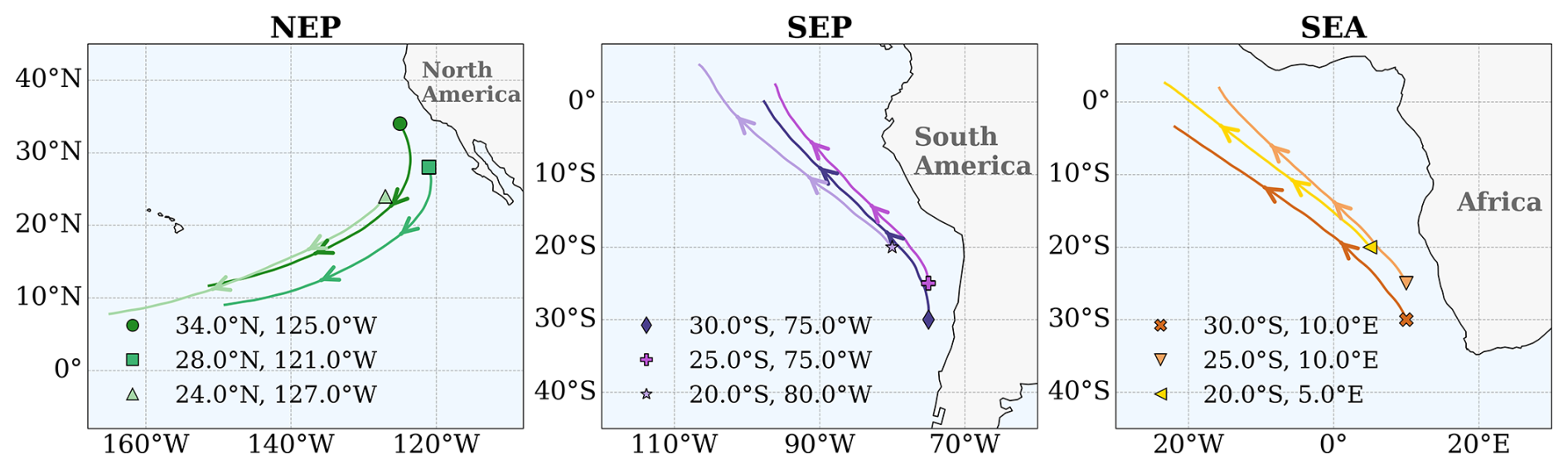
Figure 1 Mean trajectory paths across the three ocean basins: (a) Northeast Pacific (NEP), (b) Southeast Pacific (SEP), and (c) Southeast Atlantic (SEA). Each colored line represents the average trajectory path initiated from a distinct starting point, marked by a unique symbol, with arrows indicating the direction of propagation with the trade winds.

2.1.2 Trajectory setup

Forward trajectories are initialized daily at 18:00 UTC. This choice provides a consistent sampling point within the diurnal cycle, for each initiation point, helping to reduce variability associated with diurnal cloud evolution. Each trajectory runs for 8 d (192 h), which is sufficient in most cases to capture the evolution of Sc-Cu-DC as trajectories move from the subtropics toward the tropics. The dataset covers the years 2015–2019 and includes daily trajectories from nine different initiation locations for three oceanic basins: the Northeast Pacific (NEP1-3), the Southeast Pacific (SEP1-3), and the Southeast Atlantic (SEA1-3), with three initiation locations in each region (see Fig. 1). Each location, therefore, consists of 1825 daily initiated trajectories. These locations span a range of different longitudes and latitudes within each basin and are all situated along the eastern boundary of the subtropical oceans, where Sc clouds are prevalent.

The three initiation locations within each basin are not intended to represent distinct meteorological regimes, but rather to increase sampling and assess the robustness of the results to small perturbations in the initial conditions. Although the points are geographically close, the resulting trajectories diverge (Fig. 1) and sample different environmental conditions along their Lagrangian evolution (Figs. 3, S2–S9 in the Supplement).

The starting points are located along the eastern coasts of subtropical oceans, where easterly winds are found on average. Thus, trajectories initialized at these points are expected to flow predominantly westward and equatorward, toward the deep tropics. To ensure a robust analysis of cloud transitions, we apply a series of constraints to filter out trajectories that do not meet physical and meteorological criteria expected of the relevant cloud transition. This filtering method is critical in order to isolate trajectories that are representative of the tropical cloud transition and to avoid trajectories that cross over land, where the air mass would be affected by the continent.

2.1.3 Data Filtering

First, to ensure that trajectories remain representative of oceanic conditions, we apply a land fraction threshold of less than 0.01, calculated as the mean land fraction along each trajectory. This excludes trajectories strongly affected by land-atmosphere interactions. We further ensure spatial relevance by applying a poleward deviation filter: trajectories must remain on or equatorward of their starting latitude, preventing inclusion of cases that deviate from the trade wind flow, where midlatitude influences could dominate cloud evolution. Additionally, an equatorward latitude shift of at least 10° is required to capture significant meridional advection consistent with the trade wind-driven tropical cloud transition. Trajectories are also required to exhibit westward longitudinal motion of at least 5°, in line with typical large-scale flow in tropical and subtropical ocean basins.

To reduce noise and avoid highly variable environmental changes (for example, due to strong spatial meandering of the trajectory), we limit SST variability by selecting only trajectories with a standard deviation in SST below 4.0 K. This constraint helps preserve trajectories within a relatively stable increase in SST with progression towards the tropics, as expected from the tropical cloud transition. It is important to note that we do not restrict cases in which the SST decreases locally, to allow for temperature gradients caused, for example, by oceanic eddies. Together, these constraints isolate a subset of trajectories suitable for analyzing ACI across evolving tropical cloud regimes. Under this framework, all remaining trajectories exhibit upward vertical velocity and precipitate at some point along their evolution, thus representing deep convection formation at a certain time in the trajectory.

The impact that each filter has on the number of retained trajectories appears in Table S1 in the Supplement. After applying these filters, the retained trajectories numbered 760 for NEP1, 1092 for NEP2, 851 for NEP3, 1080 for SEP1, 1075 for SEP2, 1603 for SEP3, 1055 for SEA1, 871 for SEA2, and 1111 for SEA3. Across all locations, the mean number of retained trajectories is 1055 ± 242. i.e., on average, about 58 % of the data passes the filtering procedure.

2.1.4 Data Grouping

To assess the influence of aerosol loading on cloud development, we divide the valid trajectories into two groups based on aerosol optical depth (AOD), using total-column aerosol extinction as a proxy for CCN. Here, AOD is taken from MERRA-2 reanalysis rather than directly from MODIS. MERRA-2 assimilates MODIS and AERONET observations into its global model, providing a continuous aerosol field along each trajectory and avoiding the clear-sky retrieval limitations of MODIS. For each trajectory i, AOD values are extracted across all time steps, forming a time series A_i(t). We then compute the mean AOD across all N trajectories for each time step (presented in Fig. S1):

$$\begin{array}{}\text{(1)}& \stackrel{\mathrm{‾}}{A}\left(t\right)={\displaystyle \frac{\mathrm{1}}{N}}\sum _{i=\mathrm{1}}^N{A}_i\left(t\right).\end{array}$$

At every time step t, we then calculate the deviation of each trajectory from the ensemble mean, $\left(A_i\right(t)-\stackrel{\mathrm{‾}}{A}(t\left)\right)$. These time-resolved deviations are subsequently summed over the full trajectory length to obtain a single scalar value. We define this quantity here as signed deviation:

$$\begin{array}{}\text{(2)}& D_i=\sum _{t=\mathrm{1}}^T\left(A_i\left(t\right)-\stackrel{\mathrm{‾}}{A}\left(t\right)\right),\end{array}$$

which represents the cumulative difference between the trajectory's AOD and the time-dependent ensemble mean (Fig. 2). A positive D_i indicates that trajectory i tends to experience higher than average AOD levels relative to the time-evolving mean of the ensemble, while a negative D_i reflects lower than average AOD exposure. Thus, this metric captures relative aerosol loading in a way that accounts for the temporal evolution of AOD along the trajectories.

For each initiation location's dataset, we compute the median of the signed deviation values, D_median, and divide the trajectories into two AOD-based groups: those with D_i≤D_median (the clean group) and those with D_i>D_median (the polluted group). This method ensures an approximately even split of trajectories while preserving physical meaning by classifying them based on their relative aerosol exposure, without imposing arbitrary thresholds (the mean AOD over time is shown in Fig. S1). The subsequent analyses are conducted separately for the two AOD groups, within each initiation location.

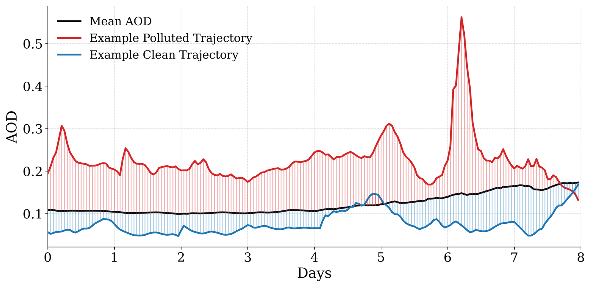
Figure 2 Time series of aerosol optical depth (AOD) for two example trajectories (from NEP1 basin), one was assigned to the polluted group (red, i=90; 1 April 2019) and one assigned to the clean group (blue, i=48; 18 February 2019), compared with the mean AOD across all trajectories (black). Vertical colored lines represent the signed deviation from the mean used in the trajectory classification.

We note that this trajectory-based classification differs from approaches that use only initial-day AOD (Christensen et al., 2020). Because our trajectories span 8 d, aerosol conditions can evolve substantially due to transport, mixing, and removal processes, making initial-day AOD potentially unrepresentative of later cloud development. The signed deviation metric, therefore, captures the relative aerosol exposure along the trajectory while accounting for its temporal evolution. We note that the increase in AOD after day 5 in the polluted example presented in Fig. 2 reflects changes in aerosol conditions along this specific trajectory driven by sea salt aerosols, probably related to an increased wind speed.

2.1.5 MODIS Cloud Retrieval Processing

MODIS cloud properties were obtained from the collection 6.1 product for Terra (MOD06_L2) and Aqua (MYD06_L2) satellites (Platnick et al., 2016) and are collocated to the trajectories. For all liquid cloud retrievals (cloud fraction, effective radius, and LWP), we retain only daytime observations with solar zenith angle <60° and sensor zenith angle <40° (to avoid pixel-swelling caused by the bow-tie effect). For cloud-top height, only the sensor-zenith filter is applied since cloud properties retrievals using the thermal channels are not affected by solar zenith angle. After screening, the hourly trajectory data are aggregated to daily means by averaging all valid retrievals across trajectories within each group (clean and polluted) for each day along the 8 d evolution. This daily-mean representation is used throughout all figures. Due to satellite overpass limitations and the applied viewing-geometry filters, MODIS sampling can be sparse. However, among the points that satisfy the viewing-geometry constraints, the vast majority contain valid retrievals (typically above 96 %); thus, missing data do not have a significant impact on the results.

2.2 Numerical Simulations

The Large-Eddy Simulation (LES) model SAM (System for Atmospheric Modeling; Khairoutdinov and Randall, 2003) is used for the simulations. To address the impact of aerosols on tropical cloud transition, simulations are conducted using an idealized Lagrangian framework (Sandu et al., 2010; McGibbon and Bretherton, 2017; Goren et al., 2019; Erfani et al., 2025), based on the mean trajectory derived from each initiation location in the observational data. In doing so, we do not aim to exactly reproduce the observed mean evolution, acknowledging the nonlinear relationship between individual trajectory behavior and their ensemble-mean response, but to represent observational-based idealized evolution. The model simulates the emerging cloud evolution under two vertically uniform CCN levels of 800 and 20 cm⁻³, assuming a supersaturation of 1 %. This wide range of aerosol conditions is useful for establishing physical understanding and is not intended to mimic the observed difference. The simulations use a two-moment bulk microphysics scheme (Morrison et al., 2005) and the RRTM radiation scheme (Mlawer et al., 1997). It is important to note that the aerosols are not prognostic in our simulations.

The domain size is chosen to be 57.6 km × 57.6 km with 147 stretched vertical levels extending up to 33 km. Vertical grid spacing is finer (tens of meters) in the lower atmosphere to better resolve boundary-layer processes and gradually increases with height. Horizontal grid spacing is 200 m × 200 m. We use a time step of 2 s and a radiation time step of 30 s. This configuration balances the need for a sufficiently large spatial domain to resolve mesoscale cloud structures and dynamics while still resolving small-scale cloud processes at LES resolution, enabling us to capture the full tropical cloud transition (Seifert and Heus, 2013; Jansson et al., 2023). To assess the sensitivity of the results to domain size, we performed an additional simulation with a larger domain (102.4 km × 102.4 km) at the same horizontal resolution (200 m × 200 m), as shown in Fig. S62. The results are qualitatively consistent with the baseline configuration, indicating that the chosen domain size does not substantially affect the main conclusions. This larger domain is comparable to the 1°×1° grid box of the observational data.

We apply small temperature perturbations (𝒪(0.02 K)) near the surface at the beginning of the simulation to initiate boundary-layer turbulence and allow initialization of convection. To ensure cloud presence at the start of the simulations, we initialized the model with a supersaturation of 1 % at the midpoint of the cloudy layer during the first hour of the simulation. Humidity increased linearly from the surface up to 1 % supersaturation at the cloudy layer midpoint, then decreased linearly back to the background value at the top of the cloudy layer. This step is not intended as a physical representation of supersaturation but as a practical initialization procedure to produce early cloud development consistent with the observed conditions along the Lagrangian trajectories.

Model Initial Conditions and Large-Scale Forcing

To simulate the cloud evolution along the mean trajectory, the model is configured using preprocessed, trajectory-mean observational data. This data provides surface and atmospheric properties, as well as large-scale forcing conditions. The variables are derived from the observation datasets and processed to align with the SAM input format. The model is initialized and forced using a combination of surface conditions, atmospheric profiles, and large-scale dynamical parameters. Surface forcing includes SST, sensible and latent heat fluxes, and surface momentum flux, with the latter prescribed as a constant value of 0.0784 m² s⁻², following Siebesma et al. (2003). Atmospheric initial conditions are based on vertical profiles of pressure, potential temperature, specific humidity, and horizontal wind components (zonal and meridional). The evolution of atmospheric temperature and humidity profiles along the clean simulations is shown in Fig. S63, for reference.

To impose realistic large-scale forcing, vertical velocity (w) was derived from the observed pressure velocity (ω) using the relation:

$$\begin{array}{}\text{(3)}& w=-{\displaystyle \frac{\mathit{\omega }}{\mathit{\rho }\cdot g}},\end{array}$$

where ρ is the air density (kg m⁻³) and g is the gravitational acceleration (9.81 m s⁻²). Additionally, large-scale wind forcing is represented by prescribing the observed zonal (u) and meridional (v) wind components. Large-scale temperature and humidity advection were not included. No nudging is applied to the dynamic or thermodynamic variables to allow them to evolve based on the local conditions (including the aerosol conditions). The initial conditions and large-scale forcing were applied homogeneously across the model domain. We therefore assume that the 1°×1° observed meteorological conditions are representative of, and apply uniformly to, the entire 57.6 km × 57.6 km LES domain.

2.3 Isolating the SST impact on q_v from the observations

To estimate water-vapor mixing ratios, q_v, in a way that accounts for temperature differences between polluted and clean groups, we first compute saturation quantities. The saturation vapor pressure over liquid water (e_s(T)) is given by:

$$\begin{array}{}\text{(4)}& e_{\mathrm{s}}\left(T\right)=\mathrm{611.2}\exp \left[{\displaystyle \frac{\mathrm{17.67}(T-\mathrm{273.15})}{T-\mathrm{35.85}}}\right],\end{array}$$

according to Bolton (1980) (Eq. 10), where T is the air temperature. The corresponding saturation mixing ratio (q_s(T,p)) is given by:

$$\begin{array}{}\text{(5)}& q_{\mathrm{s}}(T,p)={\displaystyle \frac{\mathit{\epsilon }{e}_{\mathrm{s}}\left(T\right)}{p-(\mathrm{1}-\mathit{\epsilon })e_{\mathrm{s}}\left(T\right)}},\mathit{\epsilon }=\mathrm{0.622},\end{array}$$

where p is the air pressure. For the polluted group, we include a uniform offset, ΔT, based on the location's SST difference, to represent the observed warmer temperature background. This procedure is applied only to the polluted group to normalize it by the ΔT and compare it with the clean group.

The reconstructed water vapor mixing ratio for each trajectory is obtained as:

$$\begin{array}{}\text{(6)}& q_{\mathrm{v}}^{\left(grp\right)}(z,n,t)={\mathrm{RH}}^{\left(\mathrm{grp}\right)}(z,n,t)q_{\mathrm{s}}\left(T_{\mathrm{ref}}^{\left(\mathrm{grp}\right)}(z,t),p^{\left(\mathrm{grp}\right)}(z,n,t)\right),\end{array}$$

where the relative humidity (RH) is used in fractional form and the result is expressed in g kg⁻¹. Here, “grp” denotes the trajectory group (clean or polluted). This approach isolates the role of relative humidity (RH) from that of temperature: polluted-clean differences can thus be attributed either to the background temperature (via ΔT) or to humidity anomalies independent of temperature.

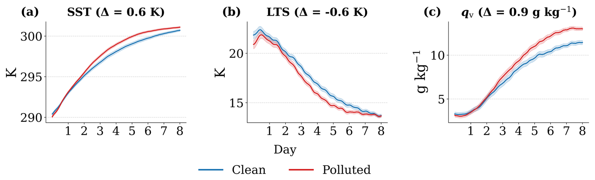
Figure 3 Hourly mean evolution of environmental variables from MERRA-2 reanalysis data along Lagrangian trajectories for the NEP1 initial location (starting from 34.0° N, 125.0° W), separated into clean (blue) and polluted (red) groups. Shown are: (a) sea surface temperature (SST), (b) lower-tropospheric stability (LTS), and (c) specific humidity at 850 hPa (q_v). Solid lines represent group means, shaded regions represent two-sided 95 % confidence intervals for the mean, computed as $\text{mean}\pm \mathrm{1.96}\times \text{SEM (standard error of the mean)}$ across trajectories at each hour. The time-mean differences between the polluted and clean trajectories are shown in parentheses above each panel. The rest of the initial locations are presented in Figs. S2–S9.

3 Results

3.1 Satellite Data Analysis

We start by analyzing the observational dataset to identify patterns in the evolution of polluted and clean cloud regimes. Specifically, Fig. 3 shows the evolution of key environmental variables and Fig. 4 shows cloud and radiation properties. Both figures represent the NEP1 dataset. Equivalent figures for all other initiation locations are provided in the Supplement (Figs. S2–S17), which exhibit generally consistent behavior across locations. In case differences arise, they will be explicitly mentioned.

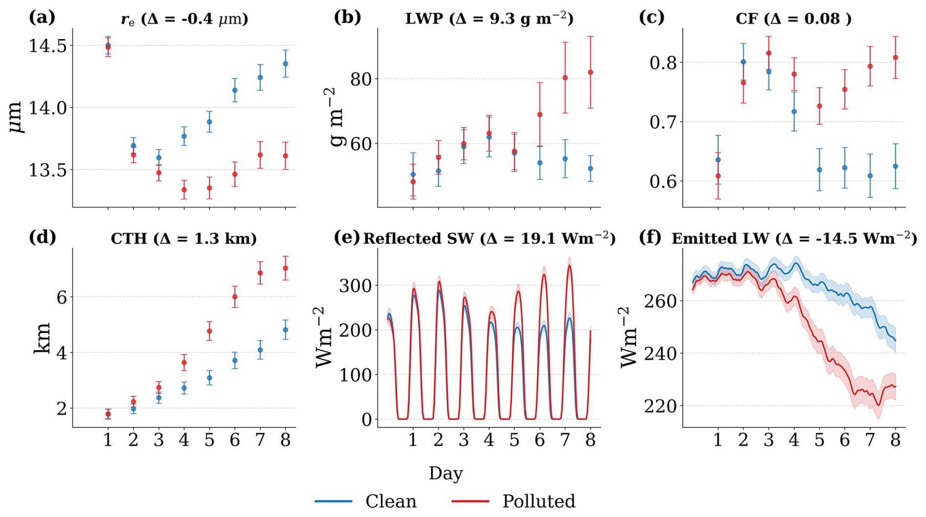
Figure 4 Mean evolution of cloud and radiation properties along Lagrangian trajectories for the NEP1 initial location (starting from 34.0° N, 125.0° W), separated into clean (blue) and polluted (red) groups. Panels (a)–(d) show daily means; panels (e)–(f) show hourly values. Shown are: (a) cloud droplet effective radius (r_e), (b) liquid water path (LWP), (c) total cloud fraction (CF), (d) cloud top height (CTH), (e) reflected shortwave radiation at top of atmosphere (Reflected SW; TOA), and (f) emitted longwave radiation at TOA (Emitted LW). Panels (a), (e)–(f) are based on CERES data, while panels (b)–(d) are based on MODIS data. Solid lines represent group means, shaded regions and error bars represent two-sided 95 % confidence intervals for the mean, computed as $\text{mean}\pm \mathrm{1.96}\times \text{SEM (standard error of the mean)}$ across trajectories at each point in time. The time-mean differences between the polluted and clean trajectories are shown in parentheses above each panel. The rest of the initial locations are presented in Figs. S10–S17.

Across both polluted and clean groups, the trajectories reflect a gradual warming of the SST (Fig. 3a), indicative of movement from the cooler subtropics toward the warmer tropics. Simultaneously, a steady decline in lower tropospheric stability (LTS; defined as the difference in potential temperature between the 700 hPa level and the surface; Fig. 3b) suggests a destabilizing boundary layer environment. Specific humidity at 850 hPa (q_v) increases markedly along the trajectories (Fig. 3c), indicating moistening of the lower free troposphere and a shift toward conditions favoring deeper convection. These thermodynamic trends are consistent with a progressive deepening of the cloud layer, as evidenced by the increasing cloud top height (CTH; Fig. 4d). Before considering aerosol differences, we note that these mean trajectories reflect the canonical tropical cloud transition.

The evolution of cloud fraction (CF; Fig. 4c) also reflects the gradual transition between cloud regimes. Initially, CF is increasing rapidly during the first day, representing the formation of extensive Sc decks during days 2–3, then declines as these decks break up into scattered Cu during days 4–5. Finally, as deep convective clouds develop in the last three days near the deep tropics, CF increases again.

As the air mass advects equatorward, LWP increases during the shallow-to-deep transition, and radiative properties respond accordingly. Specifically, as the air mass moves equatorward, the TOA emitted longwave (LW) radiation decreases steadily, reflecting the rise of cloud tops into higher and thus colder layers of the troposphere. The reflected TOA shortwave (SW) radiation is initially high (during mid-day), then declines and increases back again as deep convective systems form later in the trajectory, following generally the pattern of CF. This baseline progression provides the physical context for interpreting the differences between the clean and polluted groups. We note that during the final stage of the trajectories (days 6–8), clouds become substantially deeper, as indicated by increasing CTH, and may include mixed-phase or glaciated cloud tops. In this regime, MODIS liquid-phase retrievals such as r_e and LWP may not fully represent the cloud column and should therefore be interpreted with caution.

Having established the baseline tropical cloud transition, we now examine how aerosol loading modifies this evolution by comparing the clean and polluted groups. The polluted group exhibits generally smaller cloud droplet effective radii (r_e; Fig. 4a) compared to the clean group from the second day forward, consistent with the expected microphysical signature of the Twomey effect (Twomey, 1977). This reduction in droplet size coincides with a persistent enhancement in LWP (Fig. 4b) for polluted trajectories, especially during the last few days. The average LWP difference along the entire 8 d is 9.3 g m⁻².

Total CF (Fig. 4c) is generally higher in the polluted group around the third day and onward, indicating more extensive cloud cover in the later phases of the cloud transition. This is accompanied by a faster and more pronounced increase in CTH (Fig. 4d), with polluted trajectories reaching higher cloud tops earlier in the transition and ending with deeper convection than the clean group, with a mean difference of about 1.3 km over time.

In terms of the radiative effects in the different groups, the polluted group shows enhanced reflected TOA SW radiation (Fig. 4e) compared to the clean group, consistent with increased cloud optical thickness from smaller droplets (manifested by the decrease in r_e), and higher LWP and CF. This difference in reflected SW radiation is pronounced in the latter half of the trajectory and has a time-average difference of about 19 W m⁻². The emitted TOA LW radiation (Fig. 4f) is lower in the polluted group, especially in the later stages of the trajectory, with a time-mean difference of about −14 W m⁻², reflecting the combined influence of higher and colder cloud tops, and increased CF. These trends are consistent across all different initiation locations (Figs. S10–S17; see also Fig. 5 below).

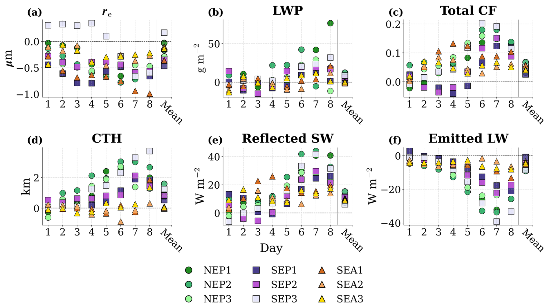
Figure 5 Daily mean differences between polluted and clean trajectory groups for all nine initiation locations (NEP1-3, SEP1-3, and SEA1-3) based on observational data. Panels show: (a) cloud droplet effective radius (r_e), (b) liquid water path (LWP), (c) total cloud fraction (CF), (d) cloud top height (CTH), (e) reflected shortwave radiation at top of atmosphere (Reflected SW; TOA), and (f) emitted longwave radiation at TOA (Emitted LW). Marker shapes and colors indicate the location: circles (NEP), squares (SEP), and triangles (SEA). The “Mean” column indicate the time-mean difference across all days.

Figure 5 provides an observational perspective on the robustness of aerosol-related cloud adjustments. Across all basins (NEP, SEP, and SEA), a generally consistent signal emerges: polluted trajectories tend to have smaller r_e (Fig. 5a; with the exception of SEP3), higher LWP from day 3 forward (Fig. 5b), larger CF (Fig. 5c), and higher CTH (Fig. 5d) compared to their clean counterparts. The reflected SW radiation at the TOA (Fig. 5e) is higher on average for polluted trajectories across all locations, reflecting the combined effect of the generally higher LWP, greater CF, and smaller droplet sizes. Correspondingly, emitted LW radiation (Fig. 5f) is lower on average in polluted cases, consistent with higher and colder cloud tops and enhanced by a larger CF. Yet these differences cannot be attributed solely to aerosol impacts, since the two groups also differ in their underlying thermodynamic environments (Figs. 3; S2–S9), reflecting potential confounding factors, i.e., co-variability with meteorological state (Gryspeerdt et al., 2019; Mülmenstädt et al., 2024; Goren et al., 2025).

The opposite r_e response in the first 5 d seen in SEP3 may reflect the influence of the coastal aerosol environment off northern Chile. This region frequently experiences strong offshore gradients in cloud microphysical properties (Wood et al., 2006; George and Wood, 2010) and episodic enhancements in sulfate outflow (Huneeus et al., 2006), which could shape the observed signal. Furthermore, satellite-retrieved AOD may include contributions from elevated aerosol layers above cloud top, which can increase column aerosol optical depth without directly affecting in-cloud microphysical processes, potentially weakening the observed cloud response (Stier, 2016; McCoy et al., 2018).

The co-variability between aerosol concentration and meteorological conditions is demonstrated in Fig. 3. While both groups follow similar overall trends fitting with the tropical cloud transition: warming SST (Fig. 3a), declining lower-tropospheric stability (Fig. 3b) and increasing q_v at 850 hPa (Fig. 3c), a systematic offset emerges between the polluted and clean groups.

Specifically, polluted trajectories exhibit slightly warmer SSTs, particularly during the mid to late stages of the cloud evolution, potentially providing a more favorable thermodynamic environment for deep convection. Here, the SST differences between the groups reflect co-variability with the large-scale meteorological and seasonal background state rather than a direct aerosol effect on SST. LTS decreases more sharply for polluted cases, implying a deepening of the inversion layer and with that, an earlier onset of deep cloud growth. q_v at 850 hPa is generally higher in the polluted group, indicating a moistening of the lower free troposphere that could enhance and sustain deep convection. These environmental differences suggest that at least part of the cloud development differences between polluted and clean trajectories (Fig. 4) may be supported or explained by variations in the environmental thermodynamic conditions. The combination of higher SSTs, reduced stability, and increased lower-tropospheric moisture in polluted trajectories creates a background state more conducive to rapid cloud deepening and larger radiative impacts.

These environmental differences between clean and polluted conditions (Fig. 3) are robust across the NEP locations (Figs. S2–S3), while the SEP locations show even larger differences, with polluted trajectories consistently warmer, less stable, and more moist (Figs. S4–S6). In contrast, the SEA locations display the opposite behavior: polluted trajectories experience slightly cooler SSTs, and more stable and drier conditions than the clean group (Figs. S7–S9), which could be driven by seasonal biomass burning from the African coast (Haywood et al., 2021; Figs. S33–S35). Notably, despite the opposite thermodynamic differences between clean and polluted conditions in the SEA region compared with the other basins, we still find a similar cloud and radiative response. Specifically, polluted conditions are characterized by smaller r_e, higher LWP, CF, and CTH, more reflected TOA SW radiation, and reduced TOA LW emission, as in the other basins (Fig. 5). The fact that the correlation between aerosol concentration and thermodynamic conditions differs between regions, yet the pattern of the polluted-clean differences in cloud and radiation properties remains consistent, suggests that these signals cannot be fully explained by environmental variability alone.

Importantly, we also find that the two groups differ in the seasonal composition (Figs. S18–S26), reflected in the number of trajectories originating from each season. These differences are indicative both of the inherent seasonality of aerosol loading in the full dataset and additional imbalances introduced by our filtering process (Sect. 2.1.3), which in turn manifests as differences in incoming solar radiation between the two groups. These seasonal differences could partly explain the observed environmental differences, even though the spatial advection paths of the trajectories remain broadly similar across seasons (Figs. S27–S35). To test whether the differences between polluted and clean groups could arise from seasonality differences, we conduct sensitivity analyses using a seasonality-controlled bootstrap. The polluted-clean differences persist even after accounting for the seasonality (Fig. S61).

The robust agreement in sign of cloud and radiative properties differences for clean and polluted conditions across diverse meteorological regimes and ocean basins, which also have different seasonality (Fig. 5), supports the interpretation that the cloud microphysical and macrophysical responses to pollution: smaller droplets, enhanced LWP, CF, and deeper clouds are robust features in our satellite record.

Using AOD as a proxy for aerosol loading has known issues (Stier, 2016; Ahn et al., 2021). Hence, sulfate aerosol mass concentration (SO₄) at the 910 hPa level was also tested as an alternative proxy for aerosol loading (as was suggested in McCoy et al., 2018; Wall et al., 2022). Both aerosol proxies (AOD and SO₄) yield generally similar cloud adjustments between polluted and clean trajectories as reported above (smaller droplet sizes, higher LWP and CF, and deeper clouds for polluted trajectories). However, using AOD as an aerosol proxy produces more pronounced differences in CTH and radiative properties across the different locations (Fig. S60). The main discrepancies between the two methods arose in the correlation between aerosols and environmental variables: for SO₄, the polluted group shows lower SST, higher LTS, and lower q_v – opposite to the AOD-based grouping (Fig. 3). Despite these environmental differences, both aerosol proxies led to consistent cloud adjustments, suggesting that the signal is generally robust to the choice of aerosol metric.

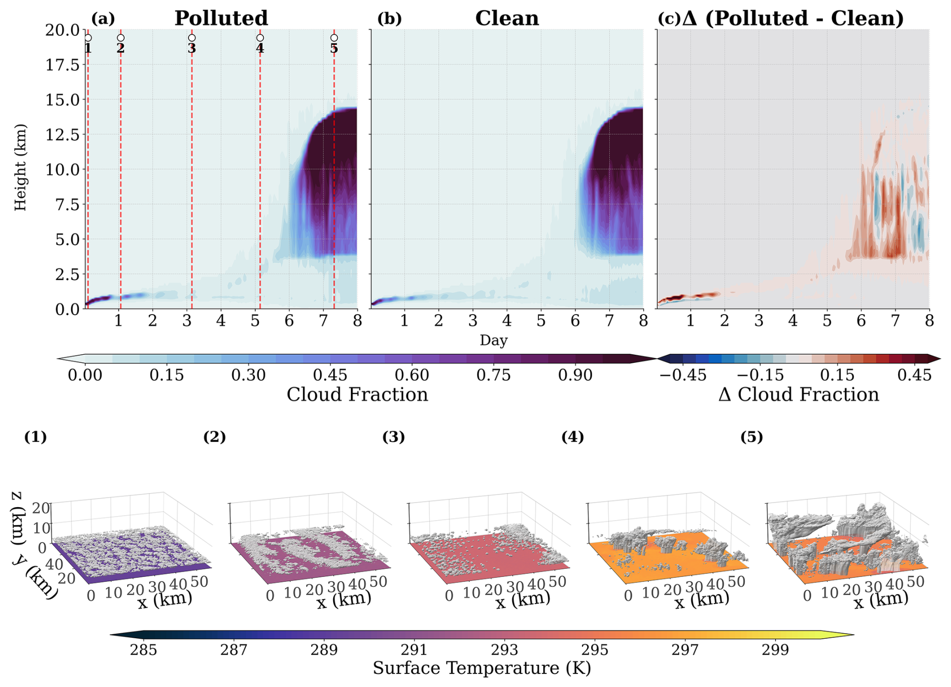
Figure 6 Hovmöller diagrams of cloud fraction evolution from model simulations for the NEP1 initial location. Panels (a) and (b) show cloud fraction as a function of height and time for the polluted and clean simulations, respectively, while panel (c) shows the difference between them. The bottom row (1–5) shows 3D cloud fields at selected timesteps corresponding to markers in panel (a), illustrating the temporal evolution of cloud structure from early development to mature convection. The rest of the initial locations are presented in Figs. S36–S43.

3.2 Numerical Simulations

To better isolate and understand the direct influence of aerosols on cloud and radiative properties, we turn to model simulations where, by construction, the aerosol influence is decoupled from the confounding meteorological factors present in the satellite data. Unlike the observations, where aerosol and meteorological effects are intertwined, the model simulations isolate the impact of aerosols by holding environmental conditions the same between polluted and clean runs. This allows the simulated cloud adjustments to be more directly attributed to aerosol perturbations.

Figure 6 shows Hovmöller diagrams illustrating the simulated evolution of cloud cover, showing the transition from Sc clouds to deep convection. At the early stages, clouds are mostly confined to the boundary layer, where shallow Sc clouds dominate below ∼ 1 km, with high CF. With time, around day 2 to 4, moistening of the lower free troposphere and gradual destabilization of the boundary layer support the breakup of Sc into scattered shallow Cu with lower CF and slightly deeper clouds, marking the transition to a more convective regime. As the lower troposphere becomes increasingly humidified, convection deepens, and cloud tops rise steadily into the mid- and upper-troposphere. During the last two days of the simulation, the domain is characterized by deep convective clouds, extending above 12 km. This progression is consistent with the canonical subtropical to tropical cloud transition.

The polluted simulation (Fig. 6a) exhibits higher CF through much of the column, particularly in the mid to upper troposphere during the later stages of the trajectory. The clean simulation (Fig. 6b) also shows cloud deepening, but with reduced vertical extent and lower mid-tropospheric coverage. Figure 6c highlights these differences, with positive anomalies (red) dominating above the boundary layer, indicating earlier and more pronounced vertical development in polluted cases. This is especially pronounced during the first two days of the cloud evolution. The earlier onset of mid-level cloudiness in the polluted group suggests a faster erosion of the capping inversion and enhanced detrainment aloft, consistent with the microphysical suppression of precipitation and associated increases in LWP and CF (Fig. 7; Albrecht, 1989; Bretherton et al., 2007; Stevens and Feingold, 2009; Erfani et al., 2022).

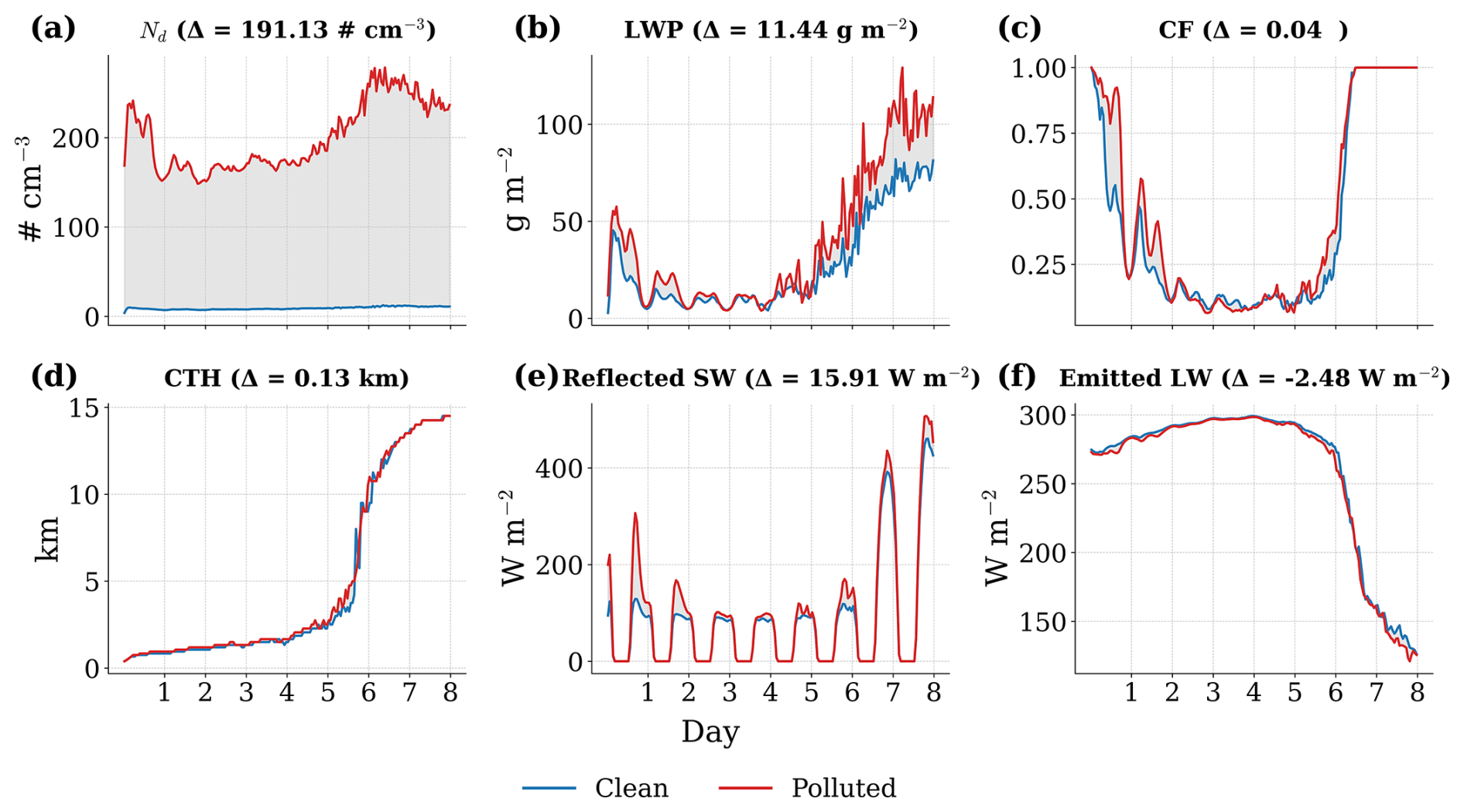
Figure 7 Hourly mean evolution of cloud and radiation variables from the model simulations for the NEP1 initial location as an example, separated into clean (blue, 20 cm⁻³) and polluted (red, 800 cm⁻³) simulations. Panels show: (a) domain mean cloud droplet number concentration (N_d), (b) liquid water path (LWP), (c) total cloud fraction (CF), (d) cloud top height (CTH), (e) reflected shortwave radiation at top of atmosphere (Reflected SW; TOA), and (f) emitted longwave radiation at TOA (Emitted LW). The time-mean differences between the polluted and clean simulations are shown in parentheses above each panel. The rest of the initial locations are presented in Figs. S44–S51.

Figure 7 shows the corresponding hourly evolution of cloud and radiation variables from the model for the same simulations presented in Fig. 6. The simulations reproduce the main observed trends: increasing LWP during the deepening of convection, decreasing CF during the Sc breakup, and recovering with the onset of deeper convection, and CTH rising as cloud systems grow deeper. These cloud changes with time are accompanied by radiative changes, including enhanced mid-day reflected SW and reduced emitted LW as cloud tops ascend into colder levels. While some differences in magnitude and timing exist compared to observations, the model captures the essential progression of tropical cloud transition. The time evolution of the simulations from the different initial locations is presented in Figs. S44–S51, and demonstrates a generally consistent behavior.

The simulated aerosol impact reproduces many of the observational signals: higher LWP, especially in the latter half of the simulation (Fig. 7b), largely similar CF (Fig. 7c), and slightly higher CTH (Fig. 7d) in polluted conditions compared to clean trajectories. The radiative responses in the model also align with the observed cloud adjustments, with polluted trajectories showing enhanced reflected SW (Fig. 7e) and slightly reduced emitted LW (Fig. 7f), which is amplified by the vertical cloud deepening (Fig. 6) and the increased high-altitude cloud cover. Together, these are indicative of optically thicker clouds with higher and colder tops, consistent with the observed trend (Fig. 4). As expected, we can also see a large enhancement in N_d (Fig. 7a), which reflects the imposed increase in CCN in the domain.

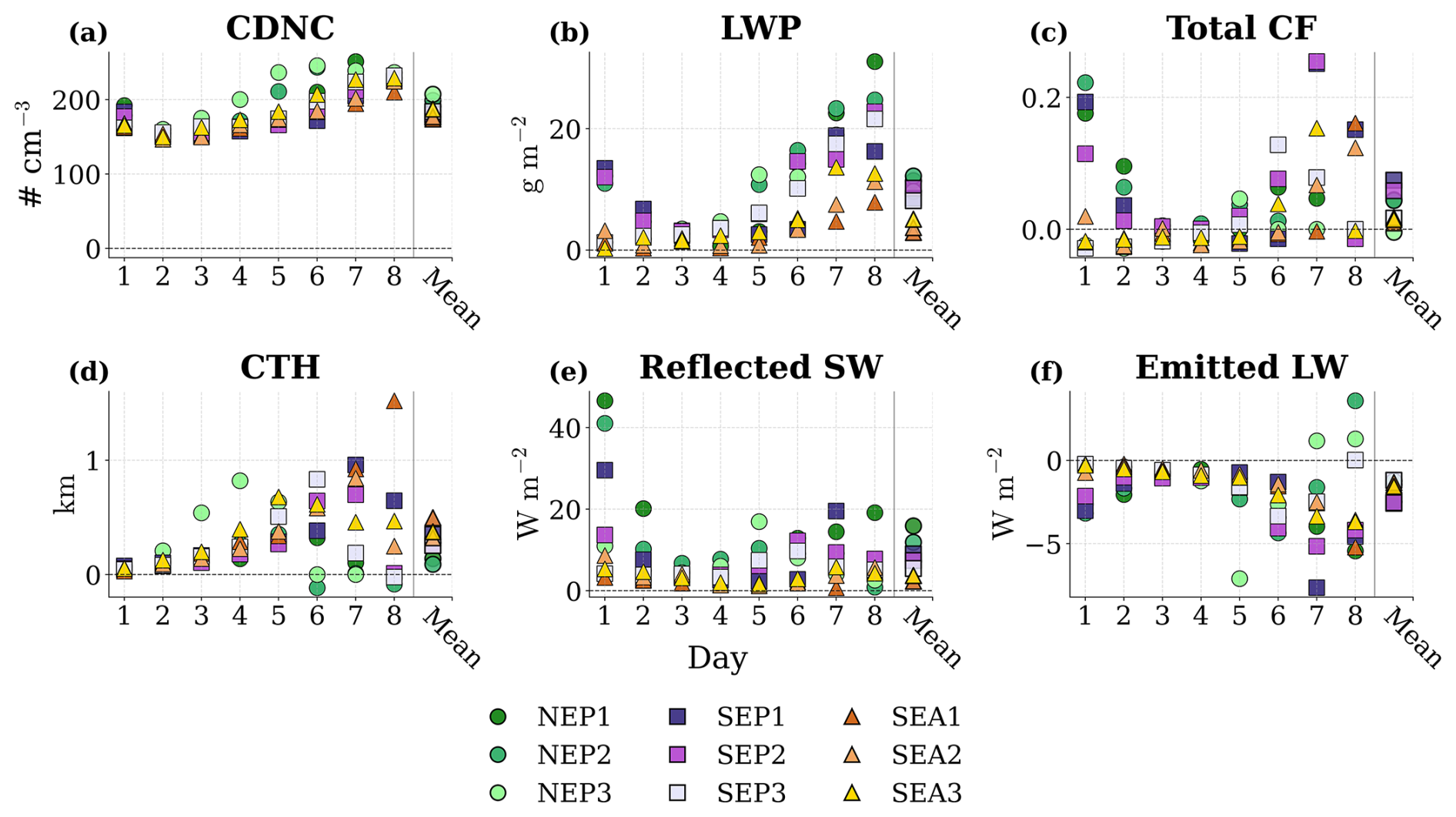
Figure 8 Daily mean differences between polluted and clean trajectory groups for all nine initiation locations (NEP1–NEP3, SEP1–SEP3, SEA1–SEA3) from model simulations. Panels show: (a) domain mean cloud droplet number concentration (N_d) (b) liquid water path (LWP), (c) total cloud fraction (CF), (d) cloud top height (CTH), (e) reflected shortwave radiation at top of atmosphere (Reflected SW; TOA), and (f) emitted longwave radiation at TOA (Emitted LW). Marker shapes and colors indicate the location: circles (NEP), squares (SEP), and triangles (SEA). The “Mean” column indicates the time-mean difference across all days.

Across all basins, the model produces a coherent signal: polluted trajectories exhibit substantially higher N_d (Fig. 8a), which propagates into enhanced LWP (Fig. 8b), larger total CF (Fig. 8c), and higher CTH (Fig. 8d). These cloud adjustments highlight the systematic influence of increased aerosol concentrations on both the horizontal and vertical extent of cloud systems. Radiative responses are similarly consistent across basins. Reflected SW at the TOA (Fig. 8e) is higher on average for polluted trajectories in all locations, consistent with optically thicker and more extensive clouds. Conversely, emitted LW at TOA (Fig. 8f) is on average lower under polluted conditions, in line with higher and colder cloud tops. The magnitudes of these differences are generally comparable to those derived from the satellite observations (Fig. 5). However, the observation-model comparison is not straightforward due to the different aerosol perturbations, with model aerosol differences larger than the observed differences.

The consistency in both the sign and the general magnitude of these simulated responses across the NE Pacific, SE Pacific, and SE Atlantic is interpreted here as the cloud and radiation changes are robust outcomes of aerosol perturbations during marine subtropical to tropical cloud transitions.

3.3 Aerosol–Environment Feedbacks

The interpretation of ACI from observations is complicated due to the co-variability between aerosol concentration and meteorological conditions. Air masses differ not only in aerosol loading but also in their thermodynamic environments (e.g., temperature, stability, humidity), making it difficult to determine whether observed cloud differences arise from aerosols or from pre-existing environmental variability (Gryspeerdt et al., 2016, 2019; McCoy et al., 2020; Christensen et al., 2021; Fons et al., 2023). Consequently, it is often assumed that the apparent cloud adjustments are strongly shaped, or even dominated, by background meteorological variability rather than the correlated aerosol influence itself (Nishant and Sherwood, 2017; Christensen et al., 2021; Wall et al., 2022; Gulistan et al., 2024).

Here, we argue that while it is well established that aerosol-meteorology co-variability can strongly influence apparent cloud responses, an additional aspect, previously discussed in the literature (Stevens and Feingold, 2009; Lee et al., 2012; Seifert and Heus, 2013; Dagan et al., 2016), deserves further attention.

Environmental changes are not only an external confounder that co-varies with aerosol loading; they may also partly arise as a consequence of aerosol impact on clouds. Previous studies have shown that aerosols can modify cloud microphysics and vertical development in ways that subsequently feed back into the surrounding atmospheric structure (Stevens and Feingold, 2009; Seifert and Heus, 2013; Dagan et al., 2016; Spill et al., 2019; Douglas and L'Ecuyer, 2020; Abbott and Cronin, 2021; Spill et al., 2021). According to this interpretation, differences in thermodynamic structure for different aerosol conditions may reflect the combined influence of large-scale meteorological variability and aerosol-induced cloud adjustments that reshape humidity, stability, and energy transport. In this context, the environment is not only a background influence on clouds, but may also be shaped by cloud responses to aerosols. Aerosols, therefore, might act as an internal driver contributing to cloud and moisture adjustments alongside the external modulation imposed by the large-scale environment.

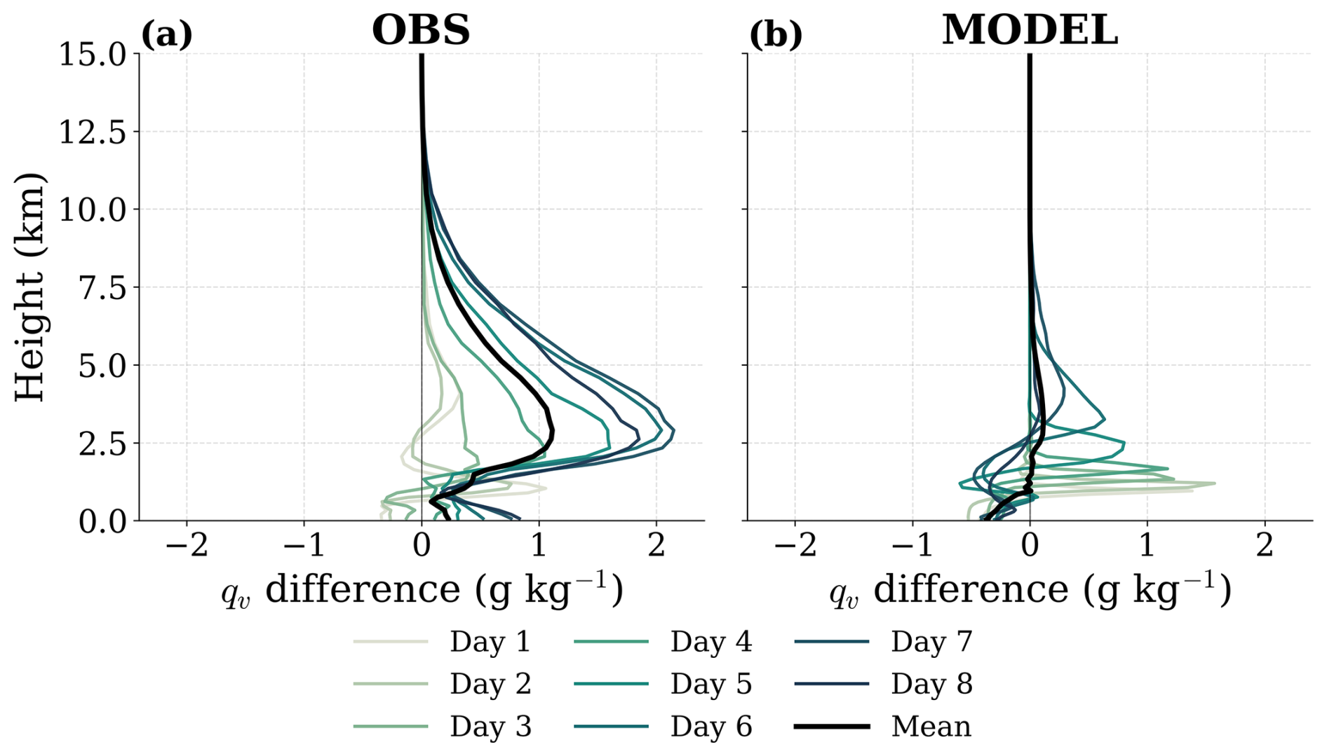
Figure 9 The difference in the vertical profile of specific humidity (q_v) between polluted and clean conditions from observations and model simulations at NEP1, as an example. Panel (a) shows the observed daily and time-mean differences (decoupled from the SST changes, see Sect. 2.3), while panel (b) shows the corresponding model results. The rest of the initial locations are presented in Figs. S52–S59.

Figure 9 demonstrates this point by showing vertical profiles of the differences in q_v between polluted and clean conditions from both observations and model simulations. Figure 9a presents the q_v profiles after accounting for SST differences between polluted and clean trajectories. Thus, they represent the humidity change, which is decoupled from the SST differences (Sect. 2.3).

In the observational record (Fig. 9a), polluted trajectories show enhanced moistening near the top of the boundary layer and into the lower free troposphere, with the signal reaching higher altitudes compared to the model results. This vertical structure is consistent with cloud deepening and detrainment of moisture aloft. In the observations (Fig. 9a), the early days (days 1–3) show relatively shallow moistening confined near the boundary layer top (∼ 1–2 km), whereas later on (days 5–8) the moist anomaly strengthens, extends and peaks at 4–6 km. This progressive deepening of the moist layer is consistent with a transition from stratocumulus-dominated conditions to more convective regimes.

The model generally reproduces this qualitative vertical structure (Fig. 9b): moistening near and above the boundary layer top, though with a smaller magnitude and a slight drying near the surface. The general agreement between observations and model simulations (where, by design, the aerosol impact is isolated from natural co-variability with meteorological conditions) is consistent with the interpretation that aerosols may contribute to shaping thermodynamic structure through cloud–environment interactions, although we cannot fully rule out the influence of co-variability with large-scale meteorology in the observational analysis. Importantly, we suggest this as a possible interpretation. We do not wish to suggest that this effect is conclusively demonstrated by our analysis.

4 Conclusions

Using five years of satellite observations combined with a trajectory model, we identified consistent differences in the evolution of cloud and radiative properties between trajectories evolving under relatively high and low aerosol loading across the Sc–Cu–DC transition, between nine distinct trajectory initiation locations spanning three ocean basins. Specifically, polluted trajectories were characterized by generally smaller r_e (mean difference of $-\mathrm{0.2}\pm \mathrm{0.1}$ µm across the nine different initial locations, where ± indicates the 95 % confidence interval of the inter-location mean), higher LWP ($\mathrm{4.0}\pm \mathrm{3.6}\mathrm{g}{\mathrm{m}}^{-\mathrm{2}}$), larger CF (0.05±0.01) and greater CTH (0.7±0.4 km) across the cloud transition. These microphysical and macrophysical cloud adjustments were accompanied by stronger reflected SW fluxes ($\mathrm{10.2}\pm \mathrm{2.0}\mathrm{W}{\mathrm{m}}^{-\mathrm{2}}$) and reduced emitted LW fluxes ($-\mathrm{5.6}\pm \mathrm{2.0}\mathrm{W}{\mathrm{m}}^{-\mathrm{2}}$; Fig. 5) at the TOA. Environmental conditions also differed between the groups, with location-specific differences: polluted trajectories were generally warmer, less stable, and moister in the NEP and SEP regions, whereas the SEA region displayed the opposite tendency. Thus, model simulations were used to better isolate the aerosol-forced response from potential meteorological confounders. Model simulations confirmed the observed trends by isolating the aerosol-forced response: polluted runs with higher LWP ($\mathrm{8.0}\pm \mathrm{2.6}\mathrm{g}{\mathrm{m}}^{-\mathrm{2}}$), CF (0.03±0.02), and CTH (0.3±0.1 km), as well as more reflected SW radiation ($\mathrm{7.4}\pm \mathrm{3.3}\mathrm{W}{\mathrm{m}}^{-\mathrm{2}}$) and less emitted LW radiation ($-\mathrm{1.8}\pm \mathrm{0.5}\mathrm{W}{\mathrm{m}}^{-\mathrm{2}}$) as observed in the satellite record (Fig. 8).

The consistency of differences between polluted and clean groups across all initiation locations, despite the diversity of their meteorological conditions, and the agreement with the model results highlight aerosols as a key factor in shaping cloud evolution along the subtropical to tropical cloud transition. The robustness of our results from both approaches (Sect. 3.1 and 3.2) is reinforced by the agreement across basins spanning both hemispheres, covering various longitudinal and latitudinal ranges, representing distinct seasonal regimes, and aerosol background. This consistency indicates that the aerosol imprint is not tied to a specific location, but rather might be a systematic feature of the tropical cloud transition.

Our results extend previous studies of ACI beyond the Sc to Cu transition (Yamaguchi et al., 2015; Goren et al., 2019; Christensen et al., 2020; Chun et al., 2025) into the full subtropical to tropical cloud transition, including deep convective development in the tropics. This broader view carries important implications. Since we concluded that aerosols modulate cloud depth, moisture, and radiative properties throughout the tropical transition, their impact is not limited to local microphysical and macrophysical processes. As previous studies have suggested, aerosols may contribute to the transport of moisture and energy within the large-scale overturning circulation, and potentially feed back on the circulation itself (Dagan et al., 2023). This non-local perspective positions aerosols not only as modulators of cloud radiative effects, but also as key players in shaping the dynamics of the tropical atmosphere.

Several limitations should be acknowledged when interpreting our results. First, while widely employed, the use of AOD as a proxy for CCN carries inherent uncertainties (Stier, 2016; Ahn et al., 2021). Satellite retrieval errors can affect AOD values above and below clouds, and retrievals are particularly uncertain in the vicinity of clouds (Koren et al., 2007). AOD is not always consistently correlated with CCN due to variations in aerosol composition, size distribution, and vertical placement relative to cloud layers.

Second, meteorological co-variability remains a fundamental challenge within the dataset. Polluted and clean trajectories differ not only in AOD but also in their thermodynamic environments (e.g., SST, LTS, and humidity). Despite our efforts, a complete separation of aerosol and meteorological influences could not be achieved with the observational data, potentially due to inherent co-variability of aerosol loading with large-scale meteorological conditions. This separation was only possible in the numerical simulations. Thus, part of the observed differences between the two groups may still reflect underlying meteorological variability.

Third, our analysis is based on 8 d Lagrangian trajectories, during which air masses can experience mixing and partial loss of their initial properties, which may alter the aerosol signal over time. However, because our dataset is made up of 5 years of daily trajectories, we expect this effect to be largely averaged out and unlikely to alter the primary patterns we identify. Nevertheless, this temporal evolution represents an inherent limitation of our observational framework.

In addition, our model simulations rely on idealized setups with prescribed CCN perturbations and a limited domain size. For example, our domain size is not sufficiently large to capture convective organization in the deep convective regime (Muller and Held, 2012). Thus, future work should examine the sensitivity of the results to the domain size. In particular, larger domains may be expected to promote earlier transitions due to the higher probability of localized precipitation events (Yamaguchi et al., 2017). However, sensitivity tests with a larger domain (Fig. S62) show very similar evolution of the bulk cloud and radiative properties, suggesting that the main conclusions of this study are not strongly sensitive to domain size, while mesoscale organization remains unresolved. In addition, future work should use prognostic aerosols, rather than prescribed CCN, and hence better represent the full spectrum of ACI and its impact on the thermodynamic conditions (Xue et al., 2010; Leung et al., 2023; Arieli et al., 2025).

Despite these limitations, the consistent aerosol signal across three ocean basins and nine initiation locations suggests that aerosol perturbations systematically amplify cloud radiative effects during the subtropical to tropical cloud transitions. This highlights how aerosols contribute to modulating tropical cloud transition and, in turn, Earth’s energy budget. More broadly, our findings suggest that assessments of aerosol–cloud–climate interactions must account not only for local adjustments in cloud microphysics and macrophysics, but also for the non-local and integrated effects of aerosols across cloud regime transitions. This perspective highlights the importance of accounting for the overarching effects that aerosols may have on the large-scale circulation in both research and climate estimations.