Evaluating turbulent and microphysical schemes in ICON for deep convection over the Alps: a case study of vertical transport and model–observation comparison

The Alpine region experiences frequent deep convection during summer, driven by thermal and mechanical forcing associated with the complex terrain. Deep convection transports moisture into the upper troposphere and lower stratosphere, which affects the climate through its radiative interactions. It is poorly represented in models that rely on parameterized convection and lack adequate representation of boundary layer turbulence and microphysics. In this study, we investigate the evolution of moist deep convection observed on 8 July 2021 over the Alps using ICON simulations with explicitly resolved convection (horizontal resolution of 1 km). The simulations use two turbulence parameterizations: the default turbulence kinetic energy (TKE) and the newly developed two turbulence energies (2 TE) scheme combined with single moment (SM) and double moment (DM) microphysics parameterizations. The simulations are evaluated using cloud properties derived from MSG/SEVIRI satellite measurements. The sensitivity of cross tropopause transport to the choice of turbulence and microphysics scheme is examined. Although, the ICON simulations capture the observed diurnal cycle of convection and successfully simulate the overshooting cloud tops during peak convective activity, our results show that the choice of the turbulence scheme influences the temporal evolution and spatial extent of deep convection, while the microphysics parameterization has a larger impact on the hydrometeor distribution and on the cross tropopause transport.

1 Introduction

Stratosphere–troposphere exchange (STE) processes play an important role in altering the chemical composition of the upper troposphere and lower stratosphere (UTLS) region, including radiatively active species such as ozone and water vapor (Holton et al., 1995). Through its radiative interaction, the stratospheric water vapor warms the troposphere and cools the stratosphere (de F. Forster and Shine, 1999; Shindell, 2001). The changes in the water vapor concentrations in the UTLS region can significantly affect the global climate (Solomon et al., 2010; Hegglin et al., 2014). The variations in stratospheric water vapor are driven by processes that occur over a broad spectrum of spatial and temporal scales. Large-scale processes are well understood and accurately represented in numerical models, but the effects of small-scale processes, like deep convection, remain incompletely understood and are not resolved in current global climate models (Benjamin et al., 2019; Palmer, 2014). The reliability of climate model projections depends on the accurate representation of these small-scale processes. Many observational and modeling studies reported the direct injection of water vapor into the lower stratosphere by overshooting convection (Fu et al., 2006; Wang et al., 2009; Wright et al., 2011). The majority of these studies have focused on the tropics. The hydration into the lower stratosphere over the tropics is linked to the variability of cold-point tropopause temperatures and the confinement strength of monsoon anticyclones in the UTLS region (Mote et al., 1996; Sherwood and Dessler, 2000; Park et al., 2007; Kumar and Ratnam, 2021). The tropical upwelling associated with the lower branch of the Brewer Dobson (BD) circulation transports this water vapor into the upper stratosphere, from where it moves poleward and descends diabatically into the extratropical lowermost stratosphere (Holton et al., 1995). The transport into the extratropical lower stratosphere from the tropical upper troposphere also occurs due to the isentropic mixing (adiabatic) associated with planetary wave activity. However, the observational studies over midlatitudes have also shown evidence of overshooting convection, which is responsible for transporting boundary layer air into the lower stratosphere (Bedka et al., 2010; Hegglin et al., 2014; Homeyer et al., 2017; Schäfler and Rautenhaus, 2023). The research on the direct injection of water vapor by overshooting convection through high resolution simulations over midlatitudes has gained considerable interest. For example, using a 2D version of Goddard Cumulus Ensemble model, Stenchikov et al. (1996) simulated a mid-latitude mesoscale convective event and found that boundary layer tracers were directly transported into the stratosphere primarily by long convective lines. Mullendore et al. (2005) performed 10 h simulations using a 3D cloud resolving model near the Kansas-Nebraska border and reported that strong core updrafts are responsible for carrying the boundary layer tracers to the lower stratosphere. The simulations over north eastern Colorado using a 3D non-hydrostatic cloud model with homogenous sounding and flat terrain revealed the pumping of CO, a boundary layer tracer into the upper troposphere by the supercell (Skamarock et al., 2000).

Most of these studies have mainly focused on the deep convective systems over relatively flat and homogeneous surfaces. However, deep convective systems frequently ocurr over complex terrain, where surface heterogeneities play a crucial role in modulating convective initiation and development. The variations in elevation, land cover and surface heating over mountainous regions can enhance low level lifting and affect the cloud formation and associated microphysical processes (Barthlott et al., 2006; Kottmeier et al., 2008). Furthermore, the intensity and vertical extent of deep convection strongly depend on surface and planetary boundary layer (PBL) fluxes controlled by soil moisture, vegetation, and canopy temperature, with a stronger influence over mountainous regions (Segal et al., 1989; Betts et al., 1994; Findell and Eltahir, 2003; Kalthoff et al., 2011; Gentine et al., 2013; Gayatri et al., 2024). Turbulence, an important sub-grid scale physical process in the surface and boundary layer, becomes more pronounced over complex terrain, as it can affect the development and strength of convection through the transport of moisture, heat and momentum. The adequate representation of turbulence is important for simulating deep convective systems, which require very fine horizontal resolution. However, current global Numerical Weather Prediction (NWP) and chemistry transport models cannot achieve this due to their coarse resolution. Several studies exist on the representation of PBL turbulence in NWP, such as those focusing on eddy-diffusivity closures, TKE-based schemes, and higher-order turbulence models (Mellor and Yamada, 1982; Moeng, 1984; Stull, 1988; Garratt, 1994). Some studies also reported the impact of turbulence schemes on deep convection, mainly focusing on storm dynamics and convective system evolution (Strauss et al., 2019; Verrelle et al., 2017; Shi et al., 2019; Hanley et al., 2015). Hanley et al. (2015) found that variations in the mixing length of the subgrid-scale turbulence scheme can significantly affect the size, intensity, and initiation time of convective storms. There are also studies which have reported the sensitivity of convection to changes in the horizontal and vertical resolutions of the model simulations (Homeyer, 2015; Jenney et al., 2023; Weisman et al., 1997; Cotton et al., 2011; Aligo et al., 2009; Keller et al., 2018; Stein et al., 2015). Using the first-order turbulence closure, Homeyer (2015) reported that storm intensity and water vapor injection into the lower stratosphere are more sensitive to horizontal resolution than to vertical resolution. In a comparative study between cloud-resolving model simulations and radar observations conducted over southern England, Stein et al. (2015) highlighted that the simulated storm type is sensitive to the mixing length used in the turbulence parameterization. They also observed some discrepancies in storm intensity and structure and suggested further refinement in the turbulence and microphysics parameterization. The NWP and climate models currently use bulk microphysics schemes, which assume a fixed shape for the size distribution of hydrometeors (e.g., cloud droplets, raindrops, ice crystals) to predict one or more bulk quantities (mass mixing ratio, number concentration, reflectivity factor or shape parameter) (Morrison et al., 2009). The majority of the previously mentioned cloud resolving simulations studies focused on single moment microphysics predicting only mass mixing ratio of the hydrometeors. The latest bulk microphysics schemes offer prediction of several moments for hydrometeor size distribution (Skamarock et al., 2019; Milbrandt and Yau, 2005).

This study primarily aims to simulate overshooting deep convection over mountainous terrain using ICOsahedral Non-hydrostatic (ICON) model, focusing on turbulence parameterization and cloud microphysics. For this purpose, hindcast simulations are performed using the ICON model coupled with RTTOV (Radiative Transfer for TOVS) and evaluated using satellite observations. The main goal of this study is to compare the performance of a recently developed two-energy turbulence scheme (2 TE scheme), which is based on modeling two distinct turbulence energies, with ICON's default TKE scheme, in representing overshooting cloud tops and the vertical transport of water vapor into the UTLS. To address this and to isolate the impact of turbulence parameterizations on these processes, sensitivity experiments are performed by changing the microphysics schemes (single-moment and double-moment), increasing vertical resolution in the UTLS, and extending the model top height. These efforts aim to advance our understanding of turbulence–convection–microphysics interactions in convection-permitting models and to contribute to the development and evaluation of the ICON framework in deep convection scenarios.

2 Methodology

2.1 Model description

The numerical simulations in the present study were carried out using the ICON model (ICON partnership (MPI-M; DWD; DKRZ; KIT; C2SM), 2024). The model solves the nonhydrostatic and compressible Navier-Stokes equations on an icosahedral-triangular grid. Such a grid structure facilitates a seamless prediction of diverse atmospheric processes, enabling the ICON model to operate effectively across global down to local scales (Zängl et al., 2015). In this study, we used the model version icon-2024.01-dwd-2.0. The simulations use two different turbulence parametrizations. The default turbulence scheme in the ICON model developed by Raschendorfer (2001) is based on a 2nd-order closure at level 2.5 according to Mellor and Yamada (1982). The second turbulence scheme is the two-energy turbulence scheme coupled to a simplified assumed probability density function method (2 TE) (Bašták Ďurán et al., 2022). The exchange of heat, moisture, and momentum between the land surface and the atmosphere is carried out by the TERRA model, developed by Schrodin and Heise (2001) and further discussed by Heise et al. (2006). Shallow convection is parametrized using a mass-flux convection scheme (Tiedtke, 1989; Bechtold et al., 2008). The radiative scheme used is ecRad (Hogan and Bozzo, 2018), which includes an atmospheric radiative transfer model and also a radiative solver that calculates the propagation of radiation through the optical medium (Deutscher Wetterdienst (DWD), 2019).

Table 1 Summary of the numerical experiments conducted in ICON.

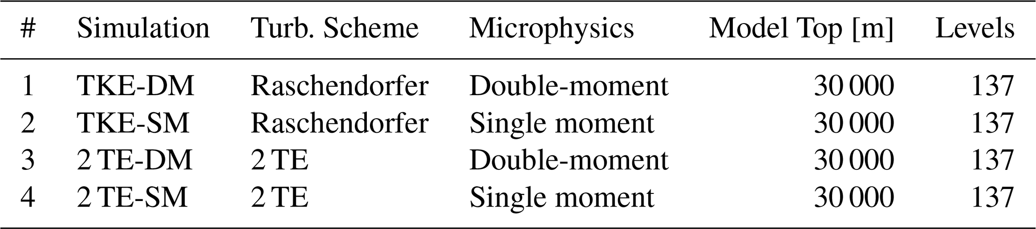
A compilation of all simulations is listed in Table 1. The simulations ran from 7 July 2021 at 18:00:00, to 9 July 2021 at 18:00:00 UTC (Local time: CEST UTC+02:00). The initial and boundary conditions were provided by the operational COSMO-1 analysis, a product from the Swiss national weather service MeteoSwiss. The boundary conditions were provided every hour. The set-up of the simulations follows the Meteoswiss operationl model, but with important modifications. The simulation domain encompasses the greater Alpine region (Fig. 1) with a horizontal grid spacing of 1 km and a time step of 10 s. The model top and sponge layer are set to 30 000 and 20 000 m, respectively, compared to 22 500 and 12 500 m in the operational configuration. In addition, the model domain is slightly smaller and the number of vertical levels is increased from 80 to 137. A vertical grid spacing of 200 m is employed in the UTLS to better capture the processes in this region. At these resolutions, convection and the diurnal cycle are well represented without the need for deep convection parameterization (Done et al., 2004; Pearson et al., 2014). The soil characteristics were provided by the Food and Agriculture organization (FAO) Digital Soil Map of the World (Sanchez et al., 2009), a comprehensive, geospatial database offering detailed information on soil types, properties, and characteristics worldwide. The orography used the Advanced Spaceborne Thermal Emission and Reflection Radiometer dataset (ASTER, Yamaguchi et al., 1998). The dataset typically offers a resolution of around 30 m. The datasets have been interpolated to match the resolution of the numerical domain which has a horizontal grid spacing of 1 km (Fig. 1).

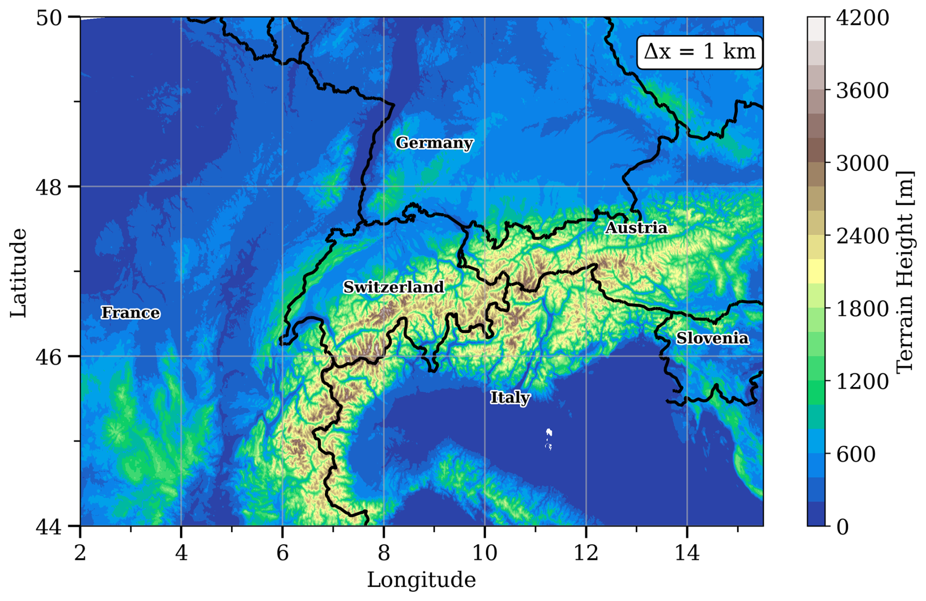
Figure 1 Topographic map of the ICON domain (colour shading) with a horizontal grid spacing of 1 km.

The ICON model employs the fast radiative transfer model (RTTOV) as the forward operator to simulate top of atmosphere radiances and brightness temperature from the atmospheric state (Saunders et al., 2018). Cloud processes were parametrized using a single-moment (Seifert, 2008; Doms et al., 2011) and double-moment (Seifert and Beheng, 2006) micro-physics (Table 1). The ICON single-moment scheme predicts five hydrometeor classes: cloud water, rainwater, cloud ice, snow, and graupel. Graupel forms through riming, where ice or snow particles collide with supercooled liquid droplets. Most microphysical processes are highly sensitive to particle size. While the mean particle size is often correlated with mass content, this correlation is not always reliable. Double-moment schemes address this limitation by predicting both the mass content and the number concentration of hydrometeors. By providing independent size information, these schemes offer a more accurate representation of particle size distributions. The double-moment option refers to the prediction of both mass content and number concentration, which are statistical moments of the particle size distribution. The double-moment microphysics scheme predicts the specific mass and number concentrations of cloud water, rain water, cloud ice, snow, graupel and hail. This scheme is suitable at convection-permitting or convection-resolving scales, i.e., mesh sizes of 3 km and finer. Only on such fine meshes the dynamics is able to resolve the convective updrafts in which graupel and hail form. As for convection, only the shallow convection parametrization is set on for the TKE simulations.

2.2 Observations

Meteosat Second Generation (MSG, Schmetz et al., 2002) comprises four geostationary satellites (Meteosat-8 to Meteosat-11) launched between August 2002 and July 2015. The main payload in the MSG satellite series is the Spinning enhanced visible and infrared Imager (SEVIRI). SEVIRI is a line-by-line optical scanning radiometer that provides continuous global images every 15 min in 12 spectral bands (4 visible and near-infrared (VNIR) and 8 infrared (IR) channels) covering a spatial range from 80° E to 80° W and 80° S to 80° N, which includes Africa, Europe, and a large portion of the Atlantic Ocean. The spatial resolution at nadir for the 11 channels, ranging from 0.6 to 14 µm at nadir, is 3 × 3 km², whereas it is 1 × 1 km² for the high resolution visible channel. The IR channels centered at 10.8 and 12 µm are used to estimate surface and cloud top temperatures. The water vapor and winds in the atmosphere are retrieved from the radiances received in the broad absorption channels at 6.2 and 7.3 µm. The visible channel is used to retrieve cloud microphysics. For details regarding the principle and the retrieval of different satellite products, the readers are referred to (Schmetz et al., 2002).

2.3 Detection of overshooting convection and ice water path

The most common method to identify the overshooting cloud top is the Brightness Temperature Difference (BTD) method (Fritz and Laszlo, 1993; Schmetz et al., 1997; Bedka et al., 2010). In this method, the difference of the brightness temperature (BT) values between the water vapor channel (WV) at 6.2 µm and the IR atmospheric window channel at 10.8 µm is calculated and is represented as BT_{(6.2–10.8 µm)}. The BT_{(6.2–10.8 µm)} is positive above deep convective overshooting clouds due to the presence of water vapour above the cloud top (Schmetz et al., 1997; Setvák et al., 2007). The water vapor present above the cloud top can emit more radiation if the temperature above the cloud top increases, leading to a warmer brightness temperature in the WV channel. The cloud top, being at a relatively lower temperature, emits less radiation, resulting in a colder brightness temperature in the IR channel, where water vapor absorption is very low. Warmer temperatures or higher water vapor amounts in the lower stratosphere above the cloud top can result in a larger positive BT_{(6.2–10.8 µm)}. The maximum difference in BTs between the WV and IR channels can range from 4 to 8 K (Schmetz et al., 1997; Setvák et al., 2007). Setvák et al. (2007) suggested that every overshooting cloud top can generate moisture, which rapidly balances its temperature with its warmer surroundings. However, the BTD method can be sensitive to cloud structure and may be influenced by thin cirrus, anvil outflow associated with deep convection, and variations in upper-tropospheric moisture (Bedka et al., 2012). In this study, SEVIRI data have been used for detecting overshooting cloud tops. To enhance the robustness of identifying overshooting cloud tops, a hybrid detection strategy that combines the BTD criterion with objectively detected mature convective cells derived from the Cb-TRAM (Cumulonimbus Tracking and Monitoring) algorithm is applied to MSG/SEVIRI observations, following the approach of Bedka et al. (2010). This method identifies three stages of thunderstorm development: stage 1 (early development), stage 2 (rapid cooling), and stage 3 (mature phase). The present analysis focuses primarily on active convective cell centers in the mature thunderstorm phase embedded within a developed anvil cirrus cloud. For these cells, the BTD is combined with texture and smoothness information derived from the reflectivity in the high resolution visible (HRV) channel of SEVIRI and BT_(6.2 µm) during daytime and nighttime, respectively. In addition, thin cirrus clouds are excluded using the brightness temperature difference, BT_{(10.8–12.0 µm)}. While stage 1 and stage 2 are usually not detectable when an anvil cloud is present from a previous or contiguous convective cell, stage 3 still could be observed: As soon as the convective cell penetrates the pre-existing anvil of another cell this newer active convective centre can be detected with Cb-TRAM even if it is not at the anvil edge or in the surroundings of the anvil. This combined BTD and Cb-TRAM approach provides more confined areas corresponding to active convective towers that can penetrate the lower stratosphere. This study focuses on satellite-based evaluation and therefore adopts a Cb-TRAM-based hybrid method, which has been extensively validated against independent observations and lightning data (Zinner et al., 2008, 2013; Merk and Zinner, 2013).Another complimentary method to detect overshooting cloud tops is to compare the tropopause temperature with IR brightnss temperature. However, this requires consistent, collocated tropopause estimates with sufficiently high vertical resolution, which are not available from the satellite observations.

The Cirrus Properties from SEVIRI (CiPS) algorithm is used to retrieve ice cloud cover (all clouds with icy tops) as well as ice optical thickness (τ) and ice water path (IWP) for thin cirrus (Strandgren et al., 2017a). CiPS is an AI-based algorithm trained with thermal SEVIRI observations and coincident cirrus properties retrieved from the Cloud-Aerosol Lidar with Orthogonal Polarization (CALIOP) instrument (Winker et al., 2009). CiPS is highly sensitive to thin cirrus but the thermal observations saturate for thick clouds in deep convection. Thus, CiPS is very well suited to derive the spatial extension of the convective clouds including their anvils, but for thicker clouds, the Algorithm for the Physical Investigation of Clouds with SEVIRI (APICS) is better suited (Bugliaro et al., 2011). APICS exploits two SEVIRI solar channels centered at 0.6 and 1.6 µm to derive the optical thickness and effective radius (r_eff) with a Nakajima-King-like method (Nakajima and King, 1990) under the assumption of ice aggregates from Baum et al. (2014).

IWP is derived under the assumption of a vertically homogeneous ice cloud layer with IWP $=\mathrm{2}/\mathrm{3}\cdot {\mathit{\rho }}_{\mathrm{ice}}\cdot r_{\mathrm{eff}}\cdot \mathit{\tau }$, where ρ_ice=917 kg m⁻³ is the density of ice. Since optical thickness ranges up to 200 and effective radius between 5 and 60 µm, maximum retrieved IWP is around 7300 g m⁻². IWP from this VIS-NIR retrieval is expected to be rather sensitive to cloud ice particles and has been shown to be similar or underestimate IWP from microwave and active observations (Rybka et al., 2021),which are sensitive to larger hydrometeors. Due to its dependence on solar observations, APICS is limited to daytime, whereas CiPS is available both during daytime and at night (for details on the algorithms, see Strandgren et al., 2017a, b; Bugliaro et al., 2011; Rybka et al., 2021). Thus, in this study, ice-cloud cover is retrieved from CiPS, while IWP is taken from APICS (daytime only). The algorithms are applied to rapid-scan data from MSG-3 (Meteosat-10) with a temporal resolution of 5 min. On 8 July 2021 the day under consideration, two data gaps occur at 11:40–12:00 and 21:10–21:15 UTC.

3 Results

3.1 Synoptic overview

In the present study, potential vorticity (PV), horizontal winds (zonal wind-u and meridional wind-v), pressure vertical velocity (ω) and geopotential height from the ERA-5 reanalysis, available at a 1 h temporal resolution and a 0.25°×0.25° horizontal resolution, are used to investigate the background synoptic-scale conditions in both the lower and upper troposphere.

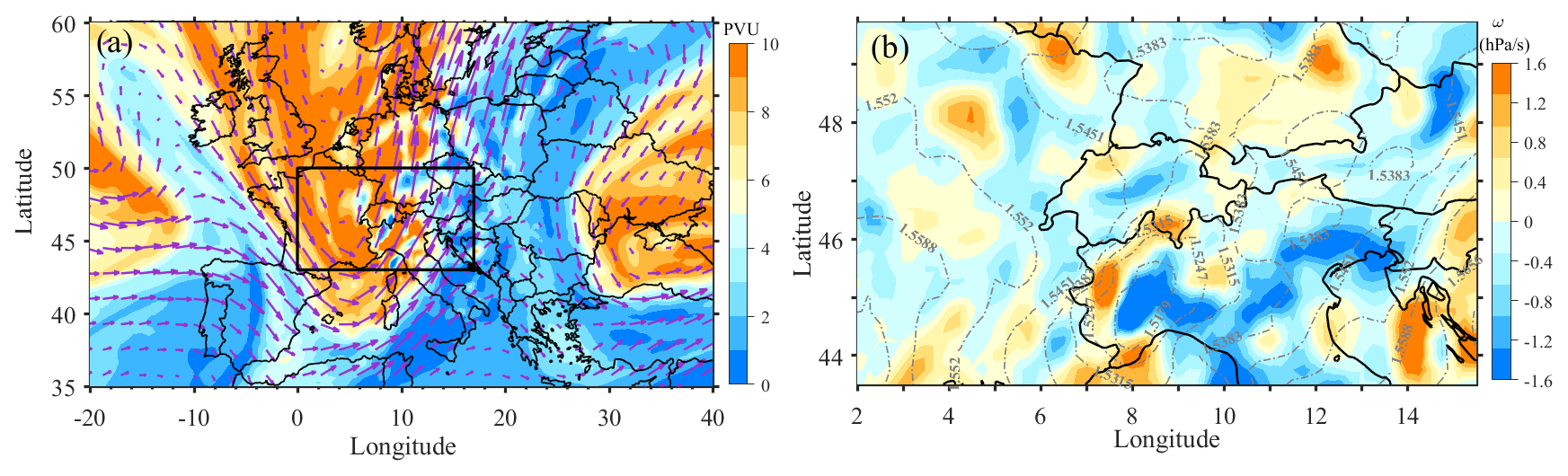
Figure 2 (a) Spatial distribution of potential vorticity (PV) along 350 K isentropic surface obtained on 8 July 2021, 15:00 UTC from ERA-5 reanalysis. The purple arrows represent the wind vectors. (b) Spatial distribution of pressure vertical velocity at 850 hPa obtained for the same time over the rectangular box region shown in (a), the dashed contour lines represent the geopotential height contours.

The 350 K isentropic surface shows a PV intrusion extending from higher latitudes to lower latitudes, covering Western and Central Europe, including France, Germany, and parts of Eastern Europe (Fig. 2). A clear cyclonic circulation is also observed from the wind circulation at this level, suggesting the presence of an upper-level trough over this region. The levels within and below the positive (cyclonic) upper-level PV exhibit a less stable potential temperature distribution (Hoskins et al., 1985; Thorpe, 1985). The PV anomalies and cyclonic circulation in the upper levels can destabilize the lower troposphere, potentially triggering deep convection over the regions ahead of the PV intrusion (Kiladis, 1998; Waugh and Funatsu, 2003). The 850 hPa geopotential height contours show a closed circulation over Central Europe, particularly near the European Alps, indicating the presence of a mesoscale low. This feature is evident by the presence of strong vertical updrafts (negative ω values), indicating strong convective active activity. The PV intrusion, associated with Rossby wave breaking, interacts with the upper-level cyclonic flow, leading to reduced static stability, enhanced upper-level divergence, and the facilitation of large-scale ascent and deep convection (Kiladis, 1998). The upper-level PV cyclonic low together with the mesoscale low in the lower troposphere can further enhance the strength of the convection, thereby leading to deep overshooting convection.

3.2 Evaluation of ICON simulations with satellite observations

3.2.1 Cloud-top temperature and diurnal cycle of convection

Figure 3 compares the simulated BT at 10.8 µm with the SEVIRI observations on 8 July 2021 at 15:00 UTC, representing the late afternoon hours when convection over the land is near its peak intensity (Chen and Houze, 1997; Yang and Slingo, 2001). Lower BTs indicate colder cloud tops, while warmer BTs correspond to low-level clouds or clear skies or thin cirrus. Satellite observations show very low BTs (< 240 K) mainly located over northern Italy, and southern Germany, eastern Switzerland, and western Austria. The simulations also capture this behavior, but with slight differences in their spatial extent and location.

To understand the diurnal evolution of convection, we analyze the temporal patterns of BT in the domain (Fig. 1) and select a region (dashed box in Fig. 3) that exhibited deep convection which developed and persisted locally, with no advection of clouds into this region from surrounding areas throughout the convective event.

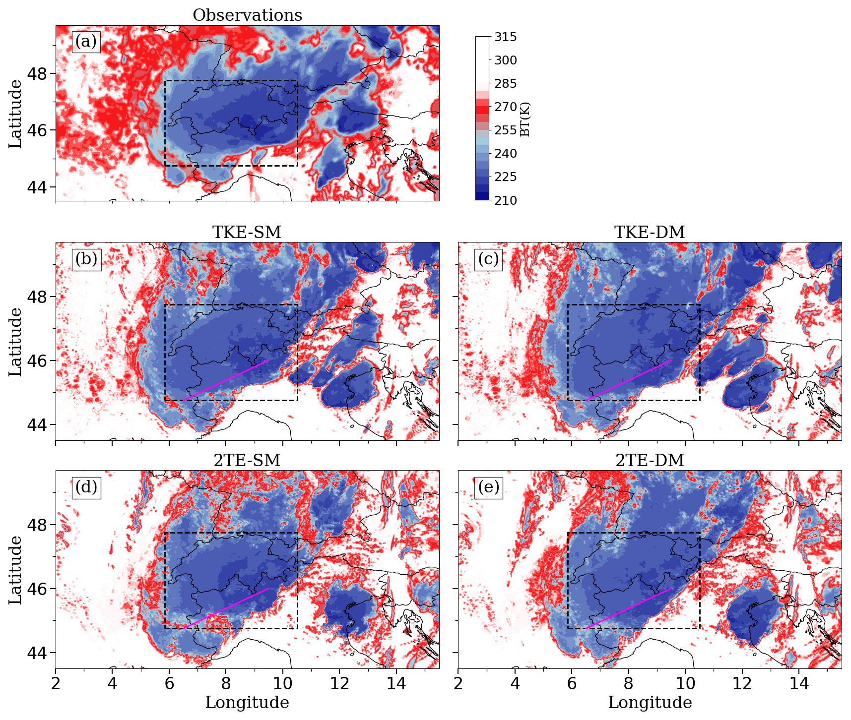
Figure 3 (a) Spatial distribution of BT obtained at 10.8 µm on 8 July 2021, 15:00 UTC (colour shading). (b), (c), (d) and (e) also represent the same but for ICON simulations. The box in all the panels represents the analysis region. Vertical cross-sections are obtained along the magenta line shown in (b), (d), (e) and (f).

During fair weather conditions, the diurnal cycle of convection is primarily driven by the surface heating and boundary layer dynamics (Weckwerth et al., 2011; Yang and Slingo, 2001; Noel et al., 2018; May et al., 2012). However, there are various mesoscale processes like anabatic winds near orography and land sea breeze ciruclation near coastal regions that can also affect the diurnal cycle of convection (Basu, 2007). The presence of a cutoff low in the upper troposphere, formed as narrow filaments from stratospheric potential vorticity (PV), as seen in this study, can also have a major impact on the triggering and evolution of the deep convection (Röthlisberger et al., 2022). The diurnal evolution of convection in simulations and observations is shown in Fig. 4, which is obtained by averaging the BT (10.8 µm) in the analysis region (44.75–47.75° N, 5.85–10.5° E). It is clear from this figure that the simulations and observations show a clear diurnal cycle of convection. During the night and early morning (00:00–09:00 UTC), higher BTs between 260 and 270 K with low fluctuations are found in simulations, indicating negligible or low convective activity. In the same time period, the observations show similar BT values; however, a small dip to 260 K between 04:00 and 07:00 UTC is likely caused by the advection of high clouds into this region during this period (not shown). A significant drop in BT is observed during the late morning and early afternoon (09:00–12:00 UTC) showing the onset of convection. The lowest BT values indicating maximum convective intensity are found during the late afternoon to evening hours (14:00–16:00 UTC), after which the BT values increase due to the decay of convective activity.

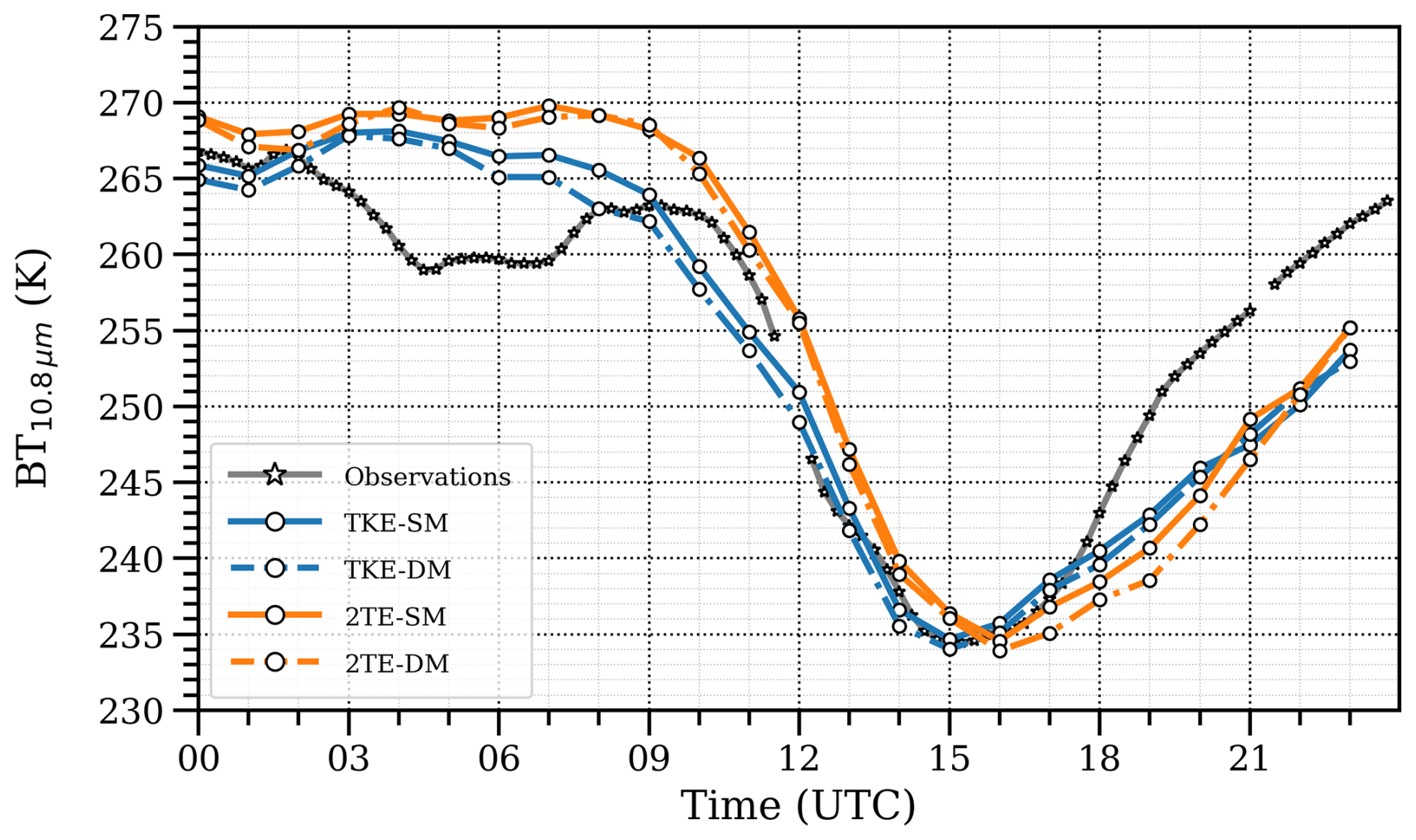
Figure 4 Time series of BT values at 10.8 µm for ICON simulations and satellite observations observed on the same day over the box region (44.75–47.75° N, 5.85–10.5° E), as shown in Fig. 3.

A sharp decrease in the BT is visible during 12:00–16:00 UTC, indicating maximum convective activity during this period. Both TKE simulations (TKE-SM & TKE-DM) match the observed timing of peak convection, reaching their minimum BT at 15:00 UTC. While the 2 TE-SM and 2 TE-DM simulations exhibit a time lag of one hour (16:00 UTC) for the peak convective activity. Signs of decay are clearly seen after 15:00–16:00 UTC; however, the simulations exhibit a slower decay of convection compared to the observations, as indicated by a slower rise in BT.

3.2.2 Overshooting convection and ice clouds

In observations, the overshooting cloud tops are identified by first using the Cb-TRAM method to detect mature convective cells, followed by applying the BT_{(6.2–10.8 µm)}>0 criterion. In model simulations, the same threshold is applied together with the identification of cloud tops penetrating above the local lapse rate tropopause. Figure 5 shows the difference in BTs obtained from satellite observations and ICON simulations at 15:00 UTC, together with the locations of overshooting cloud tops. Colder BT (Fig. 3), along with high positive BT_{(6.2–10.8 µm)}, are particularly observed in the southern, northwestern, and, to some extent, northeastern regions of the selected region in the satellite observations. The simulations broadly replicate the positive values seen in the observations for these regions, with slight differences in terms of spatial extent, intensity, and location of the maximum positive BT_{(6.2–10.8 µm)}. High BT_{(6.2–10.8 µm)} (>3 K) values are concentrated over the central Alpine region in both observations and simulations. These regions are collocated with the areas of cloud tops crossing tropopause (shown by the black dots). The spatial coverage of the moderate BT_{(6.2–10.8 µm)} values (1–3 K) is larger in simulations compared to observations. The simulations exhibit a broader distribution beyond the selected region, extending eastward and southeastward in continuous or semi-continuous streaks, in contrast to the observations, which show isolated patches. With respect to the black areas that stem from the hybdrid Cb-TRAM and BTD method, we observe that no active convective cells can be observed in Central Switzerland. This might be due to pre-existing thick ice clouds inhibiting observations of convective cloud tops or to their smaller size. In general, the black dots in the simulations in Fig. 5b–d show a lower granularity than the observations, especially for TKE.

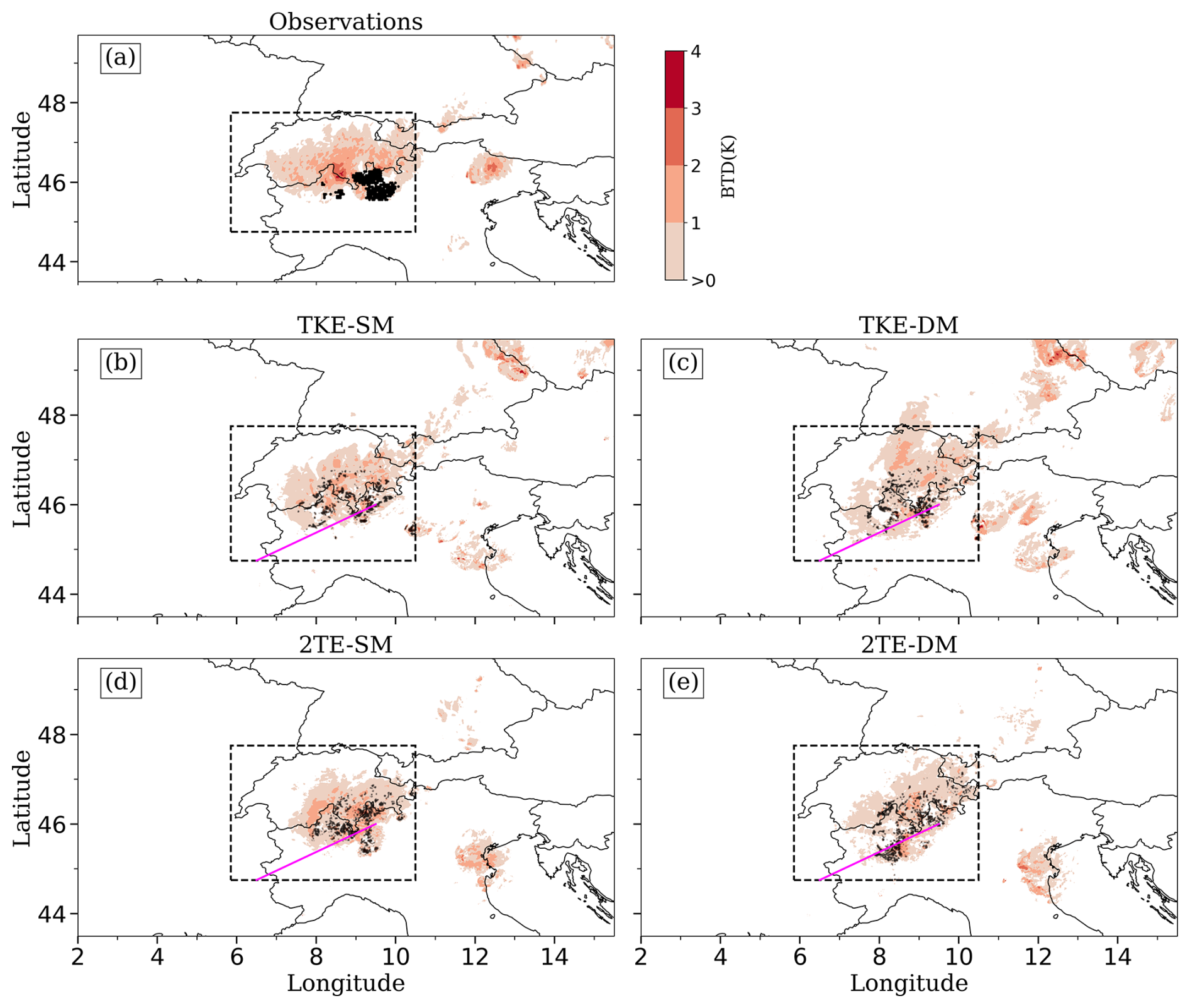
Figure 5 (a) Spatial distribution of the BT_{(6.2–10.8 µm)} obtained between WV (6.2 µm) and IR (10.8 µm) at 15:00 UTC from observations, (b), (c), (d) and (e) represent the same but for ICON simulations. The black dots in these panels indicate overshooting cloud tops identified using the common BT_{(6.2–10.8 µm)}>0 criterion, combined with Cb-TRAM method for observations and tropopause crossing criterion for the simulations. Vertical cross-sections of QI (cloud ice), QC (cloud water), w (vertical wind) and turbulent kinetic energy (tke) are obtained along the magenta line shown in (b), (d), (e) and (f).

The fractional area coverage of overshooting cloud tops in the selected region, obtained from observations, is shown in Fig. 6 along with the corresponding fractional area of cloud tops penetrating above the tropopause from simulations. Similar, to the diurnal cycle of deep convection, a strong diurnal variation in overshooting cloud tops exists in observations and simulations, with a peak between 13:00 and 16:00 UTC (afternoon to evening local time), after which it begins to decline. The percentage of the overshooting clouds is minimal early in the day (before 06:00 UTC). It can be noted from this figure that the observations showed two distinct peaks, at 08:00–09:00 and 14:00–15:00 UTC. The peak observed at 08:00–09:00 UTC seen in the observations coincided with the passage of a deep convective cell over the region, which is not found in the simulations.Despite the presence of a stable surface layer during the early morning hours, the existing PV intrusion can provide upper-level instability and dynamic lifting, thereby promoting strong convection. The overshooting cloud fraction is further amplified (Fig. 6) during the local evening hours (∼ 14:00–16:00 UTC) due to the peak associated with the diurnal cycle of surface heating, which is clearly evident both in observations and simulations.

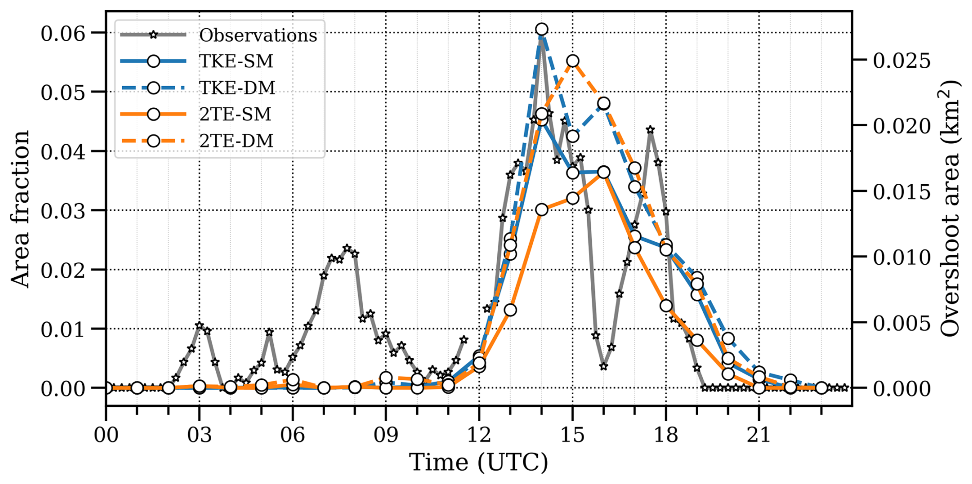
Figure 6 Time series of the area fraction of overshooting cloud tops identified using common BT_{(6.2–10.8 µm)}>0 criterion, combined with Cb-TRAM method for satellite observations and with tropopause crossing criterion for the ICON simulations, obtained on 8 July 2021 over the study region.

The TKE simulations show a sharper and more pronounced overshooting cloud fraction compared to the 2 TE simulations during this period. In particular, the DM scheme produces higher overshooting cloud tops than the SM scheme and shows better agreement with the observations. The SM scheme uses a fixed size distribution of hydrometeors, which limits the variability in the growth process of the hydrometeors.The differences observed in overshooting convection between TKE and 2 TE, as well as between SM and DM, are statistically significant (p<0.05).

In general, the auto-conversion and accretion processes are most active near the cloud top of deep convective clouds (Houze, 2014; Tao and Moncrieff, 2009). The fixed hydrometeor assumption in the SM scheme could limit the vertical development of convective anvils, thereby influencing the spatial extent of overshooting convection (Doms et al., 2011; Seifert, 2008). In contrast, the DM scheme which allows the dynamic adaptation of the hydrometeor distribution (ice particle) through auto conversion (Seifert and Beheng, 2006), exhibits a larger fractional area of overshooting convection, indicating enhanced upward transport of ice and moisture into the upper troposphere and lower stratosphere in these simulations.

The peak in the area of overshooting cloud fraction is broader in 2 TE simulations compared to TKE and observations. The difference between the observations and the model simulations is likely due to differences in the spatial resolution and retrieval methodology. Homeyer (2015) reported that the 1 km cloud-resolving simulations, performed for a convective squall line over the U.S. Central Great Plains extending from Texas to Oklahoma, captured more overshooting cloud tops than the coarser 3 km simulations and radar observations, which have a resolution of ∼ 2 km. The difference among the simulations is due to the variations in the turbulence parameterization and its influence on convective intensity and turbulent mixing, as well as model's representation of local convective processes. The observations show a distinct reduction in the area of overshooting cloud fraction at 16:00 UTC, followed by an increase during 17:00–18:00 UTC and a sharp decline thereafter. In contrast, the model simulations do not reproduce a similar pattern and instead exhibit a more gradual decrease after 14:00–16:00 UTC, particularly in the DM simulations, indicating slower dissipation and prolonged retention of convective activity.

Cloud ice constitute a large portion of the hydrometeors in overshooting deep convective systems in the upper troposphere. One important ice cloud parameter, which is also an essential climate variable, is the ice water path (IWP) (Zemp et al., 2021). The IWP represents the vertically integrated cloud ice water content, encompassing all types of ice particles. In this study, IWP is selected for comparison as it can be retrieved from satellite observations using visible channels, in contrast to quantities such as ice water content, which are available in the model output but cannot be observed by passive satellite sensors. The diurnal evolution of the IWP over the analysis region between simulations and observations is represented in Fig. 7. Higher IWP is observed in observations between 04:00 and 11:00 UTC, likely due to the advection of the high cloud tops into this region during this period. The IWP peaks around 15:00–16:00 UTC in the simulations similar to that found in observations. The TKE-DM shows a slight higher IWP compared to observations and the 2 TE simulations. The IWP obtained from 2 TE-SM is lowest. The use of DM shows an increase in the IWP values for both the TKE and the 2 TE simulations. A recent study conducted by Gettelman et al. (2024) reported that the higher IWP in the DM scheme is attributed to the enhanced ice nucleation, reduced sedimentation rates of smaller ice particles, and accretion of ice onto snow throughout the depth of the column.

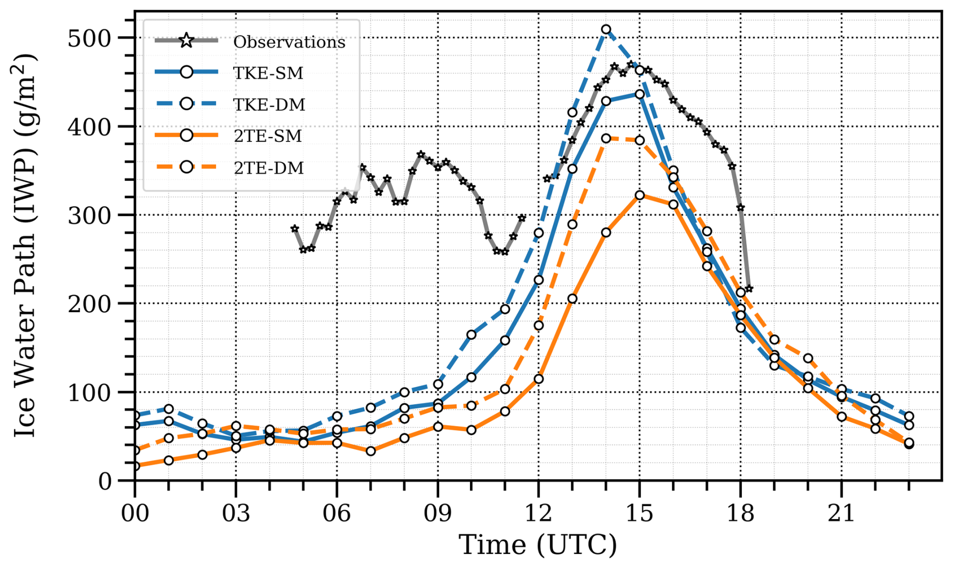
Figure 7 Time series of the Ice Water Path (IWP) between ICON simulations and satellite observations obtained on 8 July 2021 over the study region.

3.3 Impact of model setup on cross-tropopause transport and cloud ice distribution

To investigate the sensitivity of model set up on moisture transport across the tropopause, the cloud ice content (QI), water vapor content (QV) above the lapse rate tropopause (LRT), is considered, where, the LRT is defined as the lowest level at which the temperature lapse rate becomes less than 2 K km⁻¹, provided that the average lapse rate between this level and any level within the next 2 km above remains below 2 K km⁻¹ (World Meteorological Organization, 1957).

QI_LRT and QV_LRT are the integrated ice content and water vapor content in a 1 km deep layer above the LRT respectively. Their mean diurnal evolution over the analysis region is shown in Fig. 8. In all configurations, QI_LRT and QV_LRT reach a maximum between 14:00 and 15:00 UTC. This coincides with the peak in overshooting cloud fraction in both observations and simulations (Fig. 6). The DM simulations show higher QI_LRT and QV_LRT values and stronger vertical transport across the tropopause compared to single-moment (SM) simulations, likely due to differences in the representation of microphysical processes between them. The SM scheme predicts only the mass mixing ratio of the hydrometeor with a fixed particle size distribution. In contrast, the DM scheme prognostically simulates both the mass and number concentrations of hydrometeors, enabling a more realistic and dynamic representation of particle size distributions and microphysical processes such as nucleation, growth, sedimentation, and sublimation. These improvements can significantly influence the vertical transport of the hydrometeor, as the DM scheme provides a more detailed representation of phase changes and associated latent heat release, which enhance buoyancy and support deeper convective updrafts. Additionally, the DM schemes tend to produce a larger number of smaller ice particles near and above the tropopause. These particles sediment more slowly and can remain suspended for longer periods, leading to increased ice content in the upper troposphere and lower stratosphere, particularly above the LRT. This highlights the role of choice of microphysics configuration in determining the magnitude of transport into the lower stratosphere.

The differences in the mixing ratios of different water phases between the profiles averaged for the convective (14:00–16:00 UTC) and pre-convective (06:00–09:00 UTC) periods are also calculated and shown with respective to LRT in Fig. A1. High concentrations of both QI and QV are observed above the tropopause during convection compared to the pre-convective environment, confirming the effective hydration of the lower stratosphere. In particular, DM exhibits higher QV than SM both below and above the tropopause. Whereas, SM produces larger QI below tropopause than DM, possibly due to the slower conversion and sedimentation of small ice particles. In contrast, DM shows enhanced QI above the tropopause compared to SM, indicating more efficient upward transport and prolonged retention of ice in overshooting convection. QC (cloud water) is higher in DM than in SM below the tropopause, with enhanced values extending up to the tropopause, beyond which liquid water decreases sharply due to colder temperatures. Shifts in the peak altitudes of other hydrometeor profiles between SM and DM reflect variations in residence time and vertical transport, with stronger shifts observed in 2 TE than in TKE (Fig. A2). In contrast, SM shows higher QG (Graupel content) than DM in TKE simulations, whereas DM produces higher QG than SM in 2 TE, likely reflecting differences in turbulence–microphysics coupling that regulate updraft strength and liquid–ice overlap in the mixed-phase region.

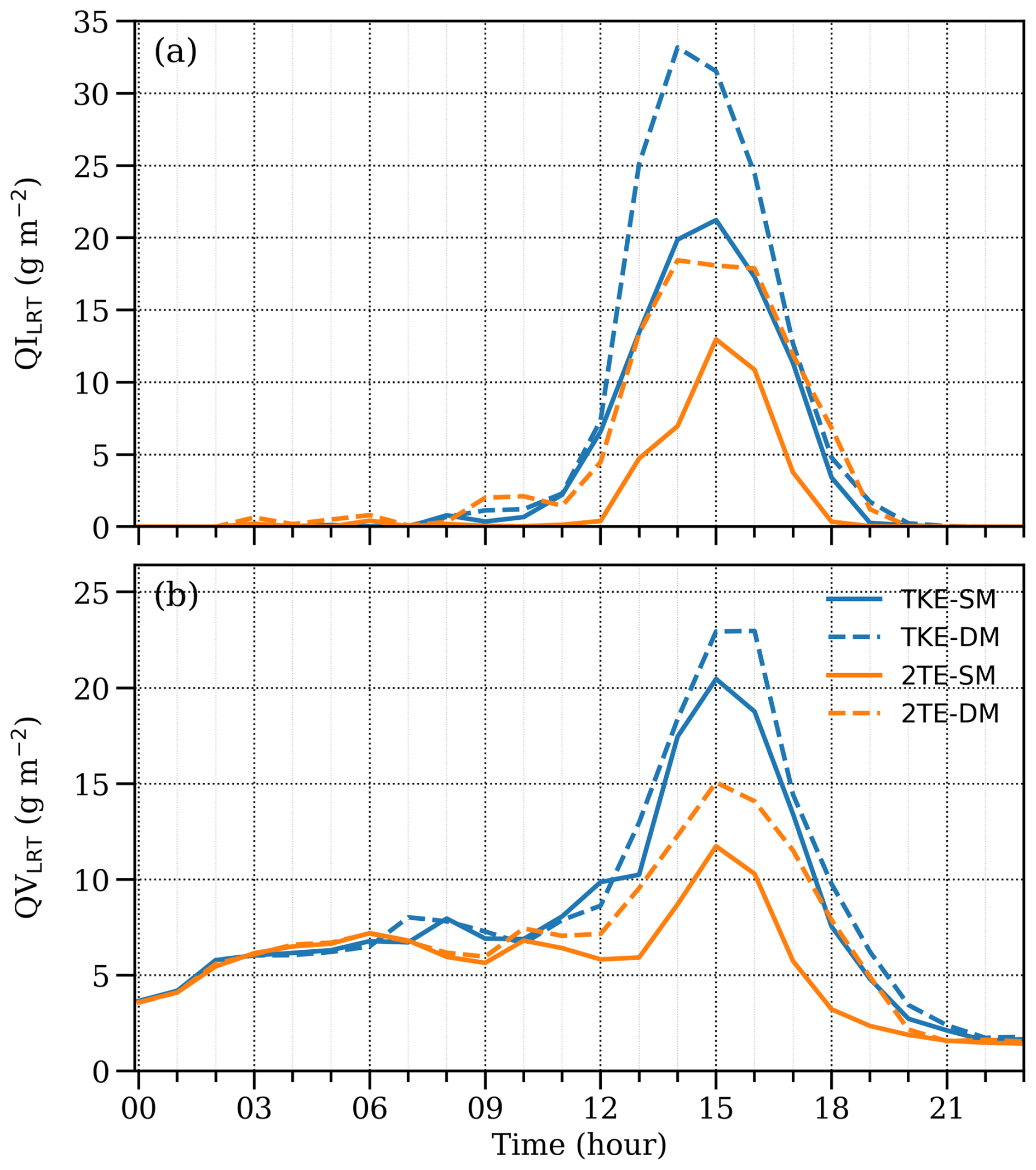
Figure 8 Time series of (a) cloud ice content (QI) above 1 km from Lapse rate tropopause, (b) water vapor content (QV) averaged over the selected region on 8 July 2021 across different simulations.

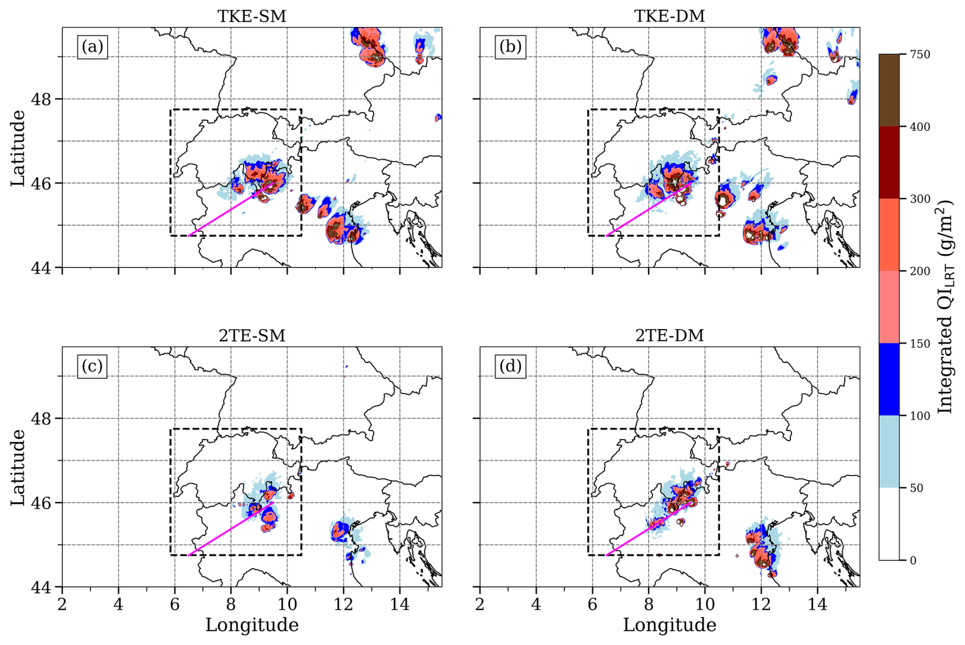
Figure 9 Spatial distribution of QI_LRT obtained at 15:00 UTC on 8 July 2021 from ICON simulations.

To understand the regional heterogeneity and spatial extent in deep convective transport, the spatial distribution of QI_LRT in different simulations for 15:00 UTC is shown in Fig. 9. The values are higher over regions with Alpine topography, indicating the influence of orographic lifting on cross-tropopause transport. From this figure, it can be observed that QI_LRT is larger in the TKE simulations, showing a higher magnitude and a broader distribution compared to the 2 TE simulations. Furthermore, the addition of the DM microphysics configuration increases the vertical transport across the tropopause, leading to higher QI_LRT values in both the TKE and 2 TE simulations. The DM simulations show more intense and frequent regions of cloud ice above the tropopause, with values exceeding 200 gm⁻². While such features are also evident in the TKE-SM simulation, they are less frequent in the 2 TE-SM configuration. This suggests that the TKE simulations support cross-tropopause transport more effectively compared to the 2 TE simulations which could be due to differences in the intensity of convection and mixing represented in the TKE and 2 TE schemes.

To investigate this, convective available potential energy (CAPE) and vertical wind at 500 hPa averaged over the analysis region are examined. The time series of the mean, 95th percentile and maximum of these parameters for both SM and DM configurations in the TKE and 2 TE simulations are shown in Fig. 10. In contrast to the 2 TE simulations, the TKE simulations exhibit higher CAPE (Fig. 10a–c) and stronger vertical wind at 500 hPa (Fig. 10d–f), indicating greater convective instability and enhanced updraft strength, which contribute to the increased transport into the UTLS region. The DM simulations show a moderate increase in CAPE and updraft strength compared to SM. So, convective and complex microphysical processes near the cloud top can influence the amount of QI_LRT.

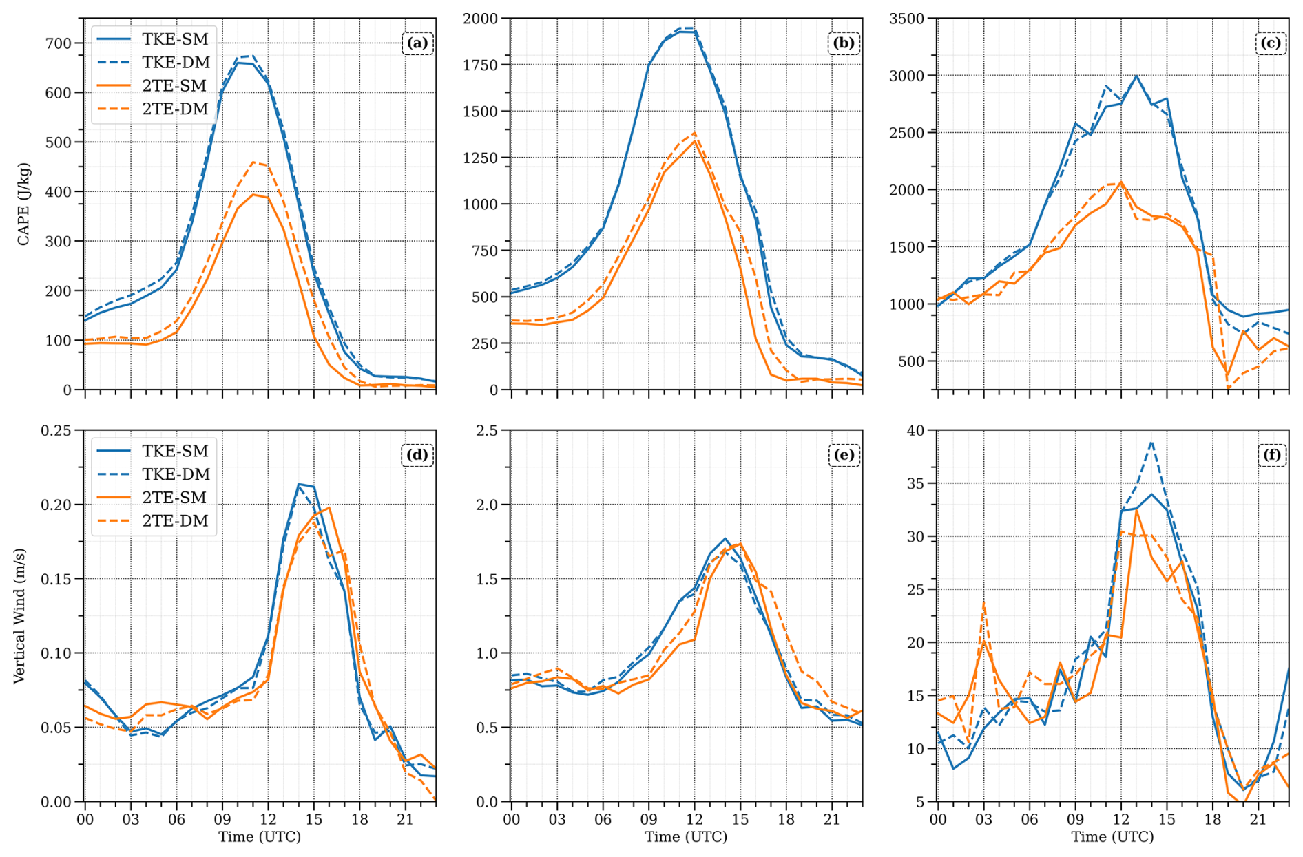
Figure 10 Time series of CAPE and 500 hPa vertical wind from ICON simulations over the box region (44.75–47.75° N, 5.85–10.5° E), as shown in Fig. 3a–c show the mean, 95th percentile and maximum of CAPE, respectively on 8 Juy 2021; panels (d)–(f) show the same statistics for vertical wind.

To investigate the role of turbulence, vertical cross sections of turbulent kinetic energy were obtained along a line (as shown in Figs. 3 and 5) passing through the main convective cores in the analysis region and is represented in Fig. 11. It is evident from this figure that the 2 TE scheme exhibits lower turbulent kinetic energy compared to the TKE simulations, indicating weaker mixing. The close spacing of potential temperature levels near tropopause is clearly observed in the TKE simulations, indicating enhanced vertical mixing due to the updrafts (Fig. 12a–b) associated with overshooting convection. Higher TKE values near and above the tropopause in these simulations could be associated with gravity wave activity. Thus, the weaker mixing and reduced convective instability in 2 TE simulations likely limited the vertical transport compared to TKE simulations. However, within 2 TE simulations, the DM scheme shows higher transport to the lower stratosphere compared to the SM simulations, possibly because of the better representation of the microphysical processes in DM compared to SM.

Horizontal advection in the deep convection anvil region can cause a temporal lag between the maximum convective activity and the amount of ice observed near the tropopause (Auguste and Chaboureau, 2022). Similar to turbulent kinetic energy, the vertical distribution of cloud ice and cloud water content in different simulations is also obtained and shown in Fig. 12. Higher cloud ice values are present in all the simulations in the altitude range of ∼ 8–12 km. It can be observed from this figure that the 2 TE-SM simulation does not show any overshooting at this particular location and time, while the implementation of DM clearly enhances the vertical transport of ice particles above LRT. The DM scheme simulations show sustained regions of cloud ice above the LRT over a larger horizontal area. This could be partly attributed to the suspension of smaller ice particles due to slower sedimentation rates and stronger updrafts. Higher cloud water values extending from the mid-troposphere to the upper troposphere are found over regions with stronger updrafts (Fig. 12), indicating the potential for moisture transport into the lower stratosphere. It can be found from this figure that the DM simulations produce higher cloud water values compared to the SM simulations possibly due to the better representation of hydrometeor mixing processes in DM compared to SM.

The LRT appears more distorted in the DM simulations compared to SM, likely due to enhanced convective activity and latent heat release, which are likely less accurately represented in the SM scheme. To summarize, the DM schemes produce more cloud water and cloud ice compared to SM in both the TKE and 2 TE simulations, indicating that the concentration of the hydrometeors and their distribution depend primarily on the choice of the turbulence parameterization.

Figure 11 Vertical Cross section of turbulent kinetic energy (m² s⁻²), along the magenta line as shown in Figs. 3 and 5 at 14:00 UTC. The black contour lines represent the potential temperature in kelvin.

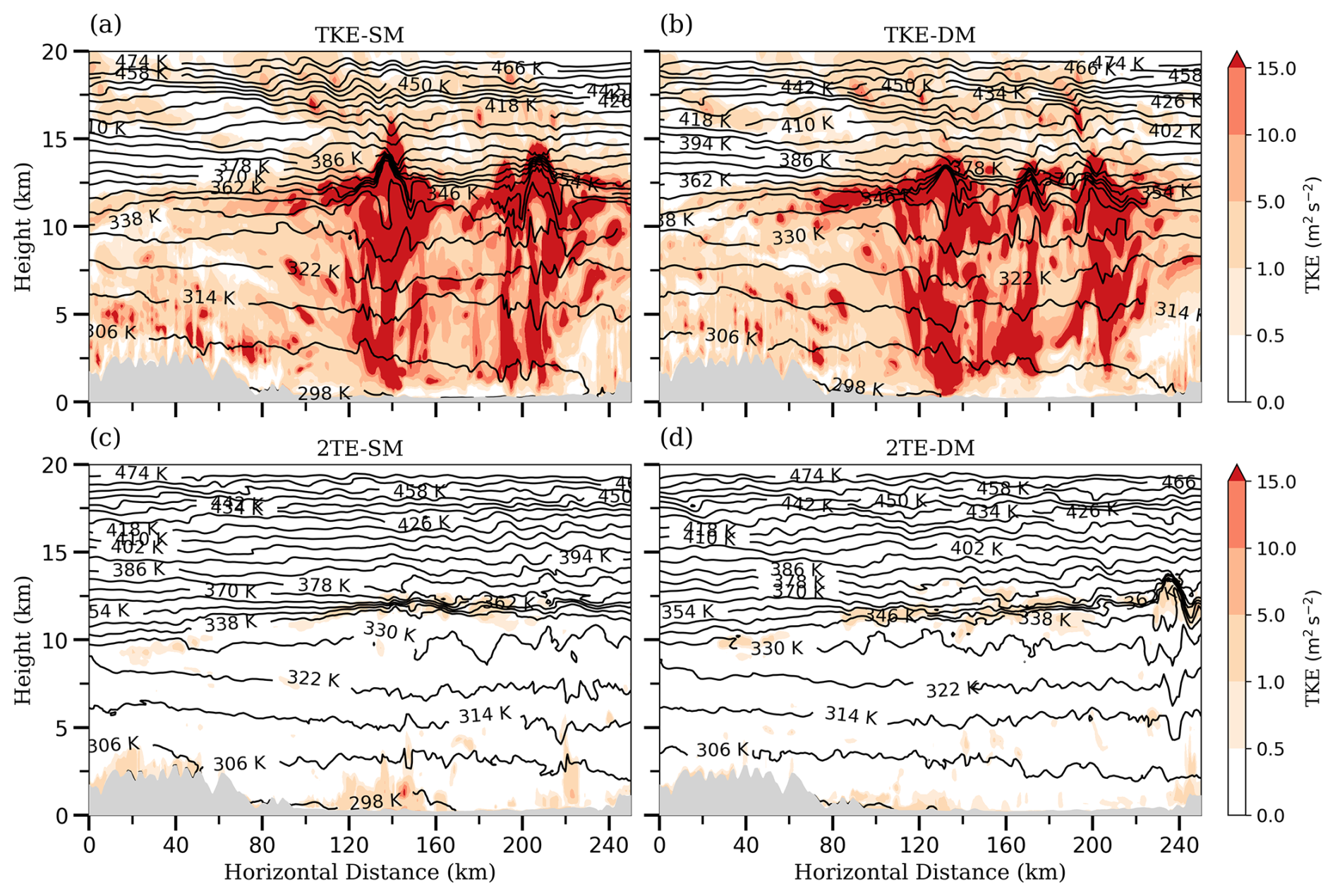
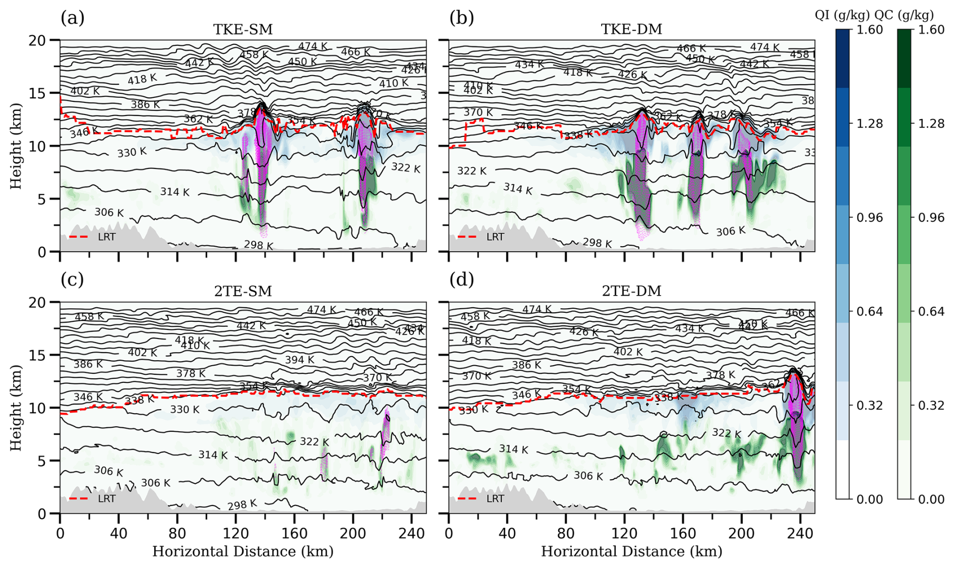
Figure 12 Same as Fig. 11 but for QI (g kg⁻¹) and QC (g kg⁻¹). The magenta lines indicate regions where vertical wind exceeds 5 m s⁻¹. The red dashed line in each panel show the altitude of the lapse rate tropopause (LRT). The black contour lines represent the potential temperature in kelvin.

4 Conclusions

This study evaluates the impact of turbulence and microphysics parameterization on the diurnal cycle of convection and the characteristics of overshooting convection in ICON simulations for a deep convective event observed on 8 July 2021 over complex terrain. Satellite observations are utilized to assess the representation of the simulated deep convection, ice clouds, ice water path and overshooting cloud tops.

The diurnal cycle of convection is evaluated by comparing the Brightness temperature (BT) values at 10.8 µm from model simulations with satellite observations. The assessment of the model simulations focused on the diurnal evolution of the overshooting cloud fraction and ice clouds, while the spatial evaluation examined the distribution of the convection and overshooting cloud tops within the domain region. For identifying the overshooting cloud tops in observations, the brightness temperature difference (BTD) method together Cumulonimbus Tracking and Monitoring (Cb-TRAM) is used. In simulations, they are diagnosed using the BTD approach in combination with the cloud area crossing the lapse-rate tropopause.

The TKE and 2 TE simulations effectively captured the diurnal cycle of convection, with the magnitude of peak convective activity (indicated by low BT values) closely matching the observations. However, differences remain, particularly in the timing of peak convective activity and the evolution of the overshooting cloud fraction, highlighting the influence of the turbulence parameterization used. The TKE simulations show a larger overshooting cloud fraction, higher IWP, and greater moisture transport into the lower stratosphere than the 2 TE simulations. This enhancement is likely due to stronger convection, as indicated by higher CAPE in TKE simulations compared to 2 TE, larger maximum vertical velocities and stronger turbulence due to higher turbulent kinetic energy. Thus, the main impact of the choice of the turbulence scheme on cloud and moisture distribution in the UTLS region is likely indirect, with its influence on the characterization and evolution of the atmospheric boundary layer being more important than its impact on mixing within deep convection. These results indicate that differences in turbulence parameterization influence the structure and intensity of deep convection and its impact on the UTLS, with important implications for stratosphere–troposphere exchange. This highlights the need for targeted sensitivity experiments to isolate boundary-layer, shallow-convection, and deep-convection interactions within the ICON framework.

There are notable differences between Double Moment (DM) and Single Moment (SM) schemes, particularly in the intensity of convection and the fraction of overshooting cloud tops. The DM scheme in both TKE and 2 TE simulations, produces more overshooting cloud tops and ice water path compared to compared to SM, indicating that the strength and vertical extent of deep convection depends on the choice of microphysics. This behavior is consistent with the findings of Gettelman et al. (2024), who demonstrated that over the Southern Ocean the DM scheme enhances the representation of supercooled liquid and ice clouds by predicting both mass and number concentrations of hydrometeors, leading to higher IWP values. values compared to the SM scheme.

Further, the sensitivity of the model setup on moisture transport into the lower stratosphere above the tropopause is also examined by estimating the integrated ice content and integrated water vapor content above 1 km from the lapse rate tropopause. It is larger using the DM scheme than the SM scheme for both the TKE and 2 TE simulations. This indicates significant differences in the vertical distribution of the hydrometeors and transport across the tropopause.

As this analysis is based on a single deep convective case over complex terrain, future work is planned to assess the sensitivity of these parameterizations across different surface conditions, including flat continental regions and oceanic environments, and under varying thermodynamic and dynamical conditions. The enhanced upper level ice and moisture transport in the DM simulations further indicates that the microphysical processes near tropopause require systematic evaluation across different convective regimes and model resolutions. Such analyses are needed to establish the broader applicability of these findings and to better constrain microphysical pathways and the representation of overshooting convection and associated transport into the lower stratosphere.

Appendix A: Additional figures

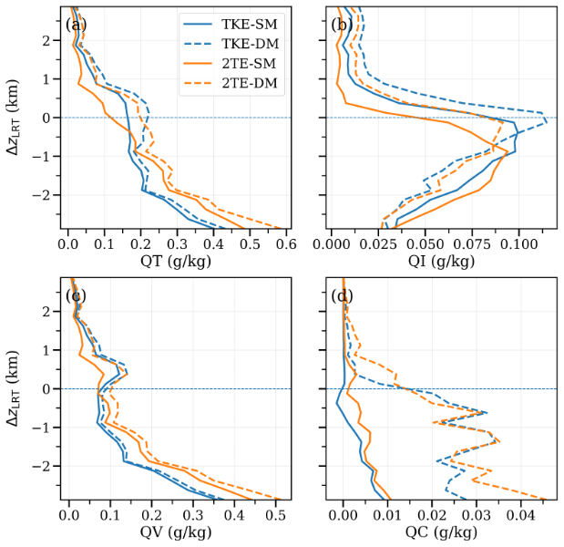
Figure A1 Mean difference between vertical profiles averaged over convective (14:00–16:00 UTC) and pre-convective environments (06:00–09:00 UTC), relative to the lapse-rate tropopause, for (a) total water (QT), (b) ice water content (QI), (c) water vapor (QV), and (d) cloud water (QC) over the selected region across different simulations. Positive values indicate enhanced mixing ratios during convective conditions.

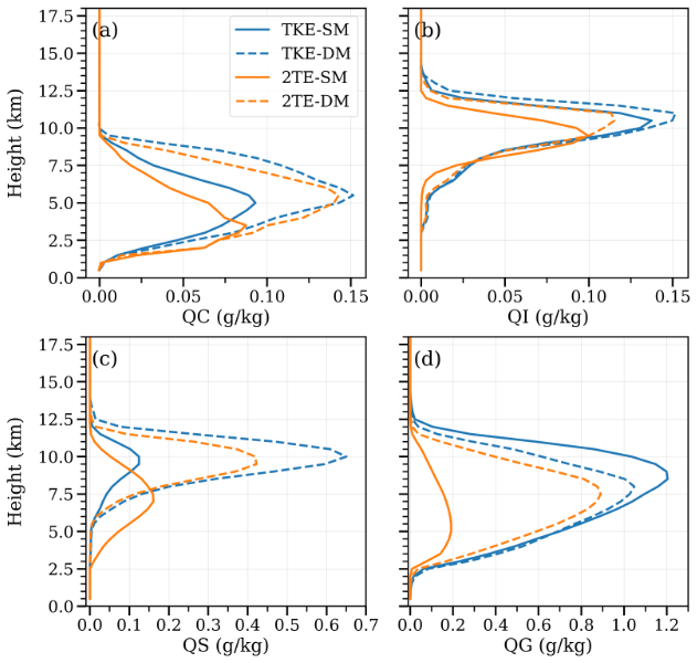
Figure A2 Mean profiles of different hydrometeors averaged over the analysis region at 15:00 UTC on 8 July 2021 across different simulations for (a) cloud water (QC), (b) cloud ice (QI), (c) snow (QS), and (d) graupel (QG).