Aerosol source apportionment modelling using a coupled regional–urban scale system

Recent air quality studies point towards the importance of distinguishing aerosol sources and their chemical composition in relation to the toxicity of particulate matter (PM). While aerosol source apportionment datasets are becoming increasingly available, model evaluations remain scarce. In this study, results from the regional-scale European Monitoring and Evaluation Programme (EMEP) Meteorological Synthesizing Centre – West (MSC-W) and coupled urban EMEP (uEMEP) Gaussian plume downscaling system are evaluated against three European positive-matrix-factorization (PMF) source apportionment datasets. These datasets are based on 28 predominantly urban measurement sites, spanning the years 2013 to 2018. In our analysis, special attention is paid to the impact of urban downscaling to 250 m resolution as well as to the role of primary and secondary organic aerosol. Results show that the model performance varies considerably between PMF factors, which may be explained in part by the ambiguity involved in the matching to modelled species and to uncertainties in the PMF analysis itself. Nevertheless, common model strengths and weaknesses can be identified. For example, model strengths relate to the ability to describe temporal variations of individual PMF factor concentrations while weaknesses relate to the apparent discrepancies in some of the underlying emission distributions. While downscaling generally improves results for road traffic and residential heating, it can also enhance existing biases, with overall model performance for these components remaining poor. Downscaling of residential heating is further found to be sensitive to the treatment of condensable wood burning emissions.

1 Introduction

Ambient particulate matter (PM) exposure is recognized as the leading environmental risk factor associated with excess mortality and morbidity (Pozzer et al., 2023). The associated health impacts have traditionally been measured in relation to the exposure to PM mass (WHO, 2021), in particular for particles with aerodynamic diameters below 2.5 µm (PM_2.5). However, recent studies suggest that PM from certain (anthropogenic) emission sources is more toxic than others, in particular in relation to their oxidative potential (OP) (Weber et al., 2021; Daellenbach et al., 2020b). Exposure to PM from anthropogenic sources is further often highest in urban areas. This points towards the general need to advance our understanding of aerosol sources, their chemical composition, and their urban-scale characteristics (El Haddad et al., 2024). In this effort, atmospheric chemistry-transport models (CTMs) play an important role in estimating PM source contributions across spatio-temporal scales. CTMs also serve as important tools for the estimation of the impacts of future emission control strategies (e.g., see The Forum for Air Quality Modelling, FAIRMODE;  Thunis et al., 2022). Critical to the use of CTMs is their validation against observationally derived data.

Many techniques have been developed to derive aerosol source apportionment from measurements (e.g., Putaud et al., 2004; Gelencsér et al., 2007; Favez et al., 2010; Yttri et al., 2011; Chen et al., 2022). The current work focuses on positive matrix factorization (PMF) analysis, which decomposes observed PM mass into contributions from individual chemical profiles (Paatero and Tapper, 1994), or so-called PMF factors. These factors may be representative of individual primary emission sources, or of chemical profiles associated with secondary aerosol formation processes. The current work focuses on the PMF datasets described by Weber et al. (2019) for total PM₁₀, Daellenbach et al. (2020b, 2017) for PM₁₀ organic aerosol (OA) and vehicular wear metals, and Chen et al. (2022) for PM₁ OA, being based on daily and hourly measurements from 28 predominantly urban sites in Europe. While the datasets each employ their own measurement and PMF protocols, there is a large degree of overlap between their identified (urban) sources.

The PMF datasets are compared against model simulations performed using the 3-dimensional Eulerian European Monitoring and Evaluation Programme (EMEP) CTM. The EMEP model (Simpson et al., 2012, 2024) has been developed for research and policy applications at Meteorological Synthesizing Centre – West (MSC-W) under the auspices of the Convention on Long-Range Transboundary Air Pollution (CLRTAP) (http://www.emep.int/mscw, last access: October 2025). In addition, PM from vehicular traffic, residential heating, and shipping emissions is downscaled to a 250 m resolution using the urban EMEP (uEMEP) Gaussian plume model (Mu et al., 2022; Denby et al., 2020). In the uEMEP model, the Local Fractions (LFs) as calculated in the EMEP model are used to downscale local emission sources without double counting of emissions (Wind et al., 2020).

Section 2 gives an overview of the EMEP/uEMEP modelling system, followed by a brief discussion of PMF analysis in Sect. 3. Given the large amount of geochemical data and measurement techniques involved in this work, a description of the matching with modelled species and emission sources is given for each dataset in an individual section (Sects. 4–6). These sections also include comparisons to model results. The overall model evaluation is summarized and discussed in Sect. 7, where special attention is paid to the treatment of condensable wood burning emissions. The results are concluded in Sect. 8.

2 Modelling system

2.1 The EMEP MSC-W model

The EMEP model version rv5.5 is used to perform regional-scale (0.1°×0.1° horizontal resolution) air quality simulations over the domain shown in Fig. 1a. The model employs 20 vertical levels up to an altitude of 100 hPa, with a surface layer approximately 45 m thick. Meteorological fields are driven by 3-hourly data from the ECMWF Integrated Forecasting System (IFS) model (ECMWF, 2014). The EMEP model is continuously evaluated against observational data within Europe (https://aeroval.met.no/pages/evaluation/?project=emep, last access: October 2025), both for hind-casting and operational purposes.

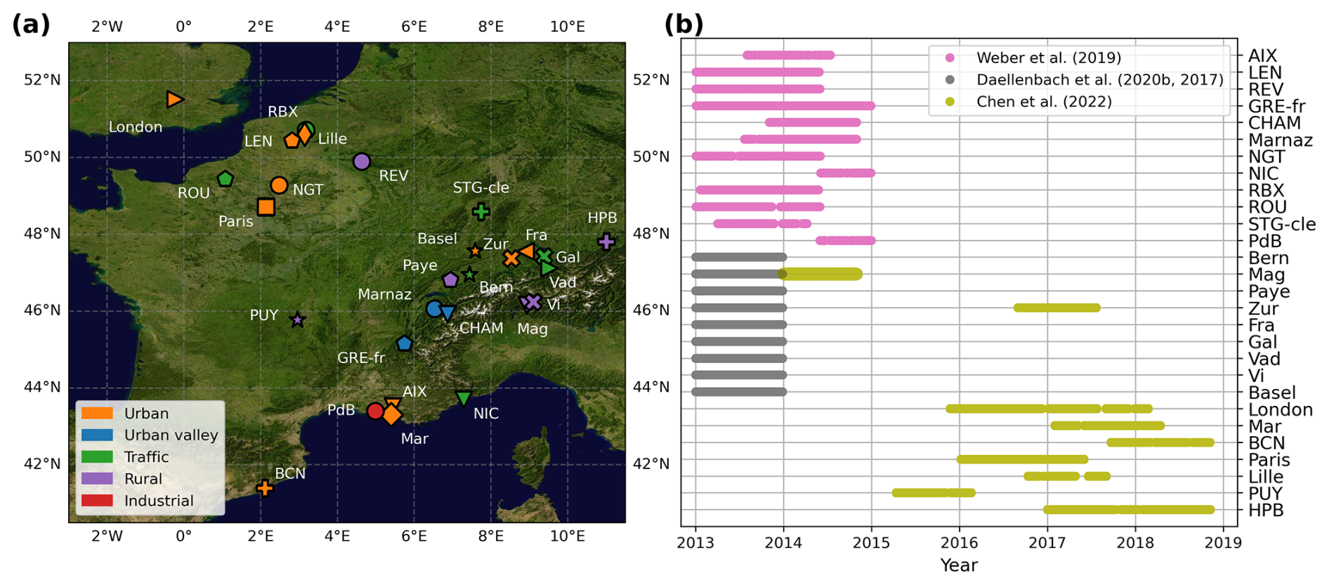
Figure 1 Panel (a) shows the geographical location and type category (indicated by their colour) of the measurement stations. Panel (b) shows the data availability and data source. Background photography in panel (a) is sourced from NASA's Earth Observatory. The marker style and colours are unique to each station, being used consistently throughout the text.

The default EmChem19 chemical mechanism is described in detail by Bergström et al. (2022), employing a set of simplified lumped VOC species to balance realism with computational complexity (Ge et al., 2024). Photolysis rates are calculated using the Cloud-J system (Prather, 2015; van Caspel et al., 2023). In the EMEP model, aerosols are represented by a fine and coarse log-normal mode, with practically all PM_2.5 being contained within the fine mode. Inorganic Secondary Aerosol (SIA, or deliquesced ${\mathrm{SO}}_{\mathrm{4}}^{\mathrm{2}-}$, ${\mathrm{NH}}_{\mathrm{4}}^{+}$, and ${\mathrm{NO}}_{\mathrm{3}}^{-}$) is calculated for fine mode aerosol using the ISORROPIA-Lite thermodynamic equilibrium module (Kakavas et al., 2022; Nenes et al., 1998). Coarse mode nitrate is formed by the heterogeneous reaction of HNO₃ on dust and sea-salt aerosol surfaces, with this fraction not contributing towards the thermodynamic equilibrium calculations. Secondary OA (SOA) formation pathways are described based on the VBS approach, including biogenic SOA (bSOA) formation by the oxidation of biogenic VOCs (isoprene, α-pinene) and anthropogenic SOA (aSOA) formation by the oxidation of benzene, toluene, and other lumped anthropogenic VOC precursor species. Total SOA mass is calculated based on the equilibrium partitioning between semi-volatile VOCs (SVOC) and total available fine-mode OA. In addition, a background OA concentration (representing missing sources of biogenic OA) is specified as 0.4 µg m⁻³ at the surface, decreasing exponentially in altitude with a 9.1 km scale-height (Bergström et al., 2012). Background OA is included as part of the fine aerosol mode, thereby contributing to the gas-particle partitioning of SVOC. It is further assumed to be comprised of highly oxygenated OM having a f_OA:OC of 2.0.

In the current work, the generalized Local Fractions (LFs) are used to track sensitivities to 1 % emission reductions for all chemical species (including those with active chemistry) for any country-and-emission-sector combination (Wind and van Caspel, 2025). These 1 % reduction sensitivities can be extrapolated to 100 % emission impacts as first-order estimates of, for example, the contribution of any given emission sector within a country to SIA across the modelling domain. For primary (inert) species, the generalized LFs calculate exact source contributions.

2.2 Default EMEP emissions

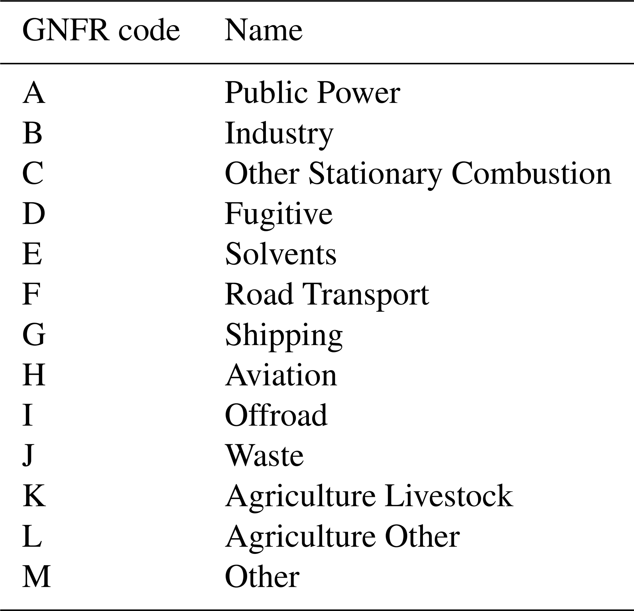
The EMEP model is run using the default gridded emissions reported by the Centre on Emission Inventories and Projections (CEIP, https://www.ceip.at/, last access: October 2025), being defined for 13 GNFR (gridded nomenclature for reporting) anthropogenic emission sectors (Table 1). This inventory includes emissions for the pollutants nitrogen oxides (NO_x), non-methane VOCs, carbon monoxide (CO), sulphur oxides (SO_x), ammonia (NH₃), primary fine particulate Matter (PM_2.5), and primary coarse PM (PM_co), which are distributed in time using a set of monthly, weekly, daily, and hourly time factors based on the CAMS-TEMPO datasets (Guevara et al., 2021, 2020). In research applications of the EMEP model, condensable primary OA (CPOA) from residential wood burning has been treated with both semi- and intermediate- volatility organic compounds (Simpson et al., 2022; Denier van der Gon et al., 2015b). The default configuration, as used here, assumes that CPOA is non-volatile, and is part of the officially reported stationary combustion (GNFR C, sometimes referred to as residential heating; even though it also includes contributions from cooking fuel use) primary PM (PPM). This assumption of inert CPOA is made to avoid usage of somewhat arbitrary VBS distributions on top of officially reported emissions. Robinson et al. (2007) and Simpson et al. (2012, 2022) have shown that this assumption has little impact on total PM_2.5 results in most areas.

Table 1 GNFR emission sector definitions.

Each of the emission sectors are combined with country-level emission split data to distribute, for example, the respective PM_2.5 emissions between the fine-mode EC, BC, and OA aerosol fractions. Stationary combustion emissions (GNFR C) further employ a temporal redistribution based on heating degree day factors, where emissions are suppressed when ambient temperatures rise above 18 °C.

The GNFR I (offroad mobile machinery) sector is by and large comprised of emissions from agriculture and forestry. Its emitted Cu per total emitted PM mass is around a factor of 10 lower than that of road transport (presumably because offroad vehicles perform less braking), based on emission data reported to CEIP. Further assuming that road abrasion and tyre wear play insignificant roles for off-road vehicles, off-road PM_2.5 OA emissions are assumed to entirely comprised of vehicular exhaust primary OA (POA). Similarly, OA emissions from the shipping sector are assumed to be entirely comprised of POA from shipping exhaust.

Natural emissions include forest fires based on the daily Fire INventory from NCAR version 2.5 (FINNv2.5, Wiedinmyer et al., 2023) dataset, as derived from the Moderate Resolution Imaging Spectroradiometer (MODIS) and Visible Infrared Imaging Radiometer Suite (VIIRS) satellite instruments. Soil-NO_x emissions are included based on the monthly climatological CAMS-GLOB-SOIL v2.4 inventory (Denier van der Gon et al., 2023), while oceanic dimethyl sulphide (DMS) emissions are included based on climatological surface water concentrations. PBAPs are included based on the parameterizations from Heald and Spracklen (2009) and Hoose et al. (2010), as described in detail by Lange et al. (2024). In short, spores emitted in the relevant size range (i.e., below a diameter of 10 µm) are approximated as having a fixed aerodynamic diameter of 5 µm, and are treated as being chemically inert. Spore emissions are controlled by the modelled specific humidity, temperature, and leaf area index (m² m⁻²). Each spore is further assumed to contain a fixed percentage of polyols by mass (4.5 %) following Vida et al. (2024). The resulting concentrations were found to compare favourably with total observed polyol concentrations in France and Norway Lange et al. (2024). All POA emissions, with the exception of those related to biomass burning (GNFR C and forest fires, with GNFR C being dominated by biomass burning), are assumed to have an f_OA:OC of 1.25 by default. For biomass burning the f_OA:OC ratio is assumed to be 1.7. Primary emissions related to plant debris are not taken into account (Brighty et al., 2022).

2.2.1 Auxiliary vehicular traffic datasets

In addition to the default emissions used in the EMEP model simulations, auxiliary datasets are employed to post-process total EMEP modelled road traffic (GNFR F) PPM concentrations into different road traffic sub-sector contributions. These auxiliary datasets contain country-total emission totals for the vehicular exhaust, brake wear, tyre wear, and road abrasion sub-sectors. To this end, the sub-sector emissions are represented as fractional contributions towards the total GNFR F emissions. These fractions are then applied to modelled GNFR F surface PPM concentrations (tracked on a per-country basis using the generalized LFs) to calculate their respective PPM contributions. A second auxiliary dataset includes chemical speciation information on a per-country basis. This provides information on the elemental carbon (EC), POA and “other minerals” content of the vehicular sub-sector emissions. The second dataset further specifies the vehicular exhaust chemical speciation data for diesel cars, diesel trucks, petrol cars, petrol 2-wheelers, and LPG vehicles individually. A third dataset provides per-country emission totals for the aforementioned vehicular exhaust sub-sectors, and can be combined with the chemical speciation data to calculate the chemical speciation split for total modelled vehicular exhaust emissions. However, since nearly all measurement sites described in the current work are urban, the contribution from diesel trucks (assumed to be predominantly associated with highway traffic) are excluded from the vehicular exhaust OA calculations. Diesel vehicles generally show considerably lower POA exhaust emissions compared to petrol vehicles. While the auxiliary dataset describing the chemical composition of the traffic sub-sector emissions is based on the year 2019, all other datasets (including the emissions used in the EMEP model) are specific to each meteorological year of simulation.

Using the road traffic auxiliary datasets, typical contributions of vehicular exhaust towards total primary road traffic PM₁₀ falls between 70 %–80 %, with the remainder being split into three nearly equal parts brake wear, tyre wear, and road abrasion. The vehicular exhaust OA fraction falls between $\mathrm{1}/\mathrm{3}$ to $\mathrm{1}/\mathrm{4}$ depending on the country-specific ratio of diesel to petrol cars. The OA fraction of tyre wear emissions is around $\mathrm{1}/\mathrm{2}$. The calculated brake wear fraction can further be used to estimate vehicular Cu and Fe concentrations. The latter are assumed to comprise 70 % of total brake wear PM₁₀ based on laboratory measurements with European legislation compliant ECE brake pads (Hagino et al., 2024).

2.3 Downscaling using uEMEP

The original LF methodology tracks the fractional contribution to PPM from emissions within so-called local regions (Wind et al., 2020). In the current work, the local regions are taken to be squares of seven 0.1°×0.1° horizontal grid-boxes wide, centred on each grid-cell of the EMEP model. The tracked local contributions to PPM are first removed from the total EMEP modelled concentrations. The EMEP grid-boxes within the local regions are then divided into 250 m² subgrids, with the local emissions being redistributed within the subgrids based on high resolution proxy data (Mu et al., 2022). Following the approach of Mu et al. (2022), road traffic (GNFR F), residential heating (GNFR C), and shipping (GNFR G) are downscaled based on Open Street Map (OpenStreetMap contributors, 2020) data, 250 m population density data from Schiavina et al. (2023), and data from the Automatic Identification System (AIS) (Kystverket, 2020), respectively. The concentration fields resulting from these downscaled emission sources are modelled using the urban EMEP (uEMEP) Gaussian plume formalism (Denby et al., 2020). For each measurement site, the contribution of the Gaussian plumes associated with each 250 m² subgrid are calculated on an hourly basis, taking into account ambient meteorological conditions. The total contribution from each subgrid is referred to as the (station total) local uEMEP contribution. Total concentrations then follow as the downscaled local uEMEP part plus the non-local EMEP part, together being referred to as the uEMEP results. We note that EMEP results for non-downscaled species are interpolated to site-specific locations based on bi-linear interpolation.

As described in Denby et al. (2020), contributions from Gaussian plumes from different uEMEP subgrids to concentrations at a single site can be used to calculate a weighted average travel time. While normally calculated for use in a simplified O₃ chemistry scheme, the weighted travel time is calculated in the current work in relation to downscaled PM₁₀ (Sect. 7.1).

3 PMF analysis

PMF analysis is an inverse modelling technique that decomposes measurements describing total PM mass into (positive) contributions from a number of chemical profiles, or so-called PMF-factors (Reff et al., 2007). This is achieved by solving a system of the form

$$\begin{array}{}\text{(1)}& x_{i,j}=\sum _{m=\mathrm{1}}^n{w}_{i,m}{f}_{m,j}+{\mathit{\epsilon }}_{i,j},\end{array}$$

where x_i,j represents the contributions of j number of chemical species to measurements indexed by i. Measured contributions are apportioned between n different PMF factors (f), where the weights of the factors are represented by w_i,m. ε_i,j represents the residual of the solution. The solution for w can then be used to construct time series of the different PMF factor concentrations. In the PMF analysis, factor profiles can be pre-defined based on existing knowledge of emission sources and other chemical processes, or they may be derived as unconstrained factors. In general, however, PMF factors are derived based on the temporal covariance of its different chemical components. External constraints on the PMF solution can also imposed, for example with the use of chemical tracer species and other co-located measurement data.

Details about the PMF techniques employed by the datasets are given in their respective sections, including a discussion of their uncertainty estimates. In general, both the measurement input data, optimal PMF solution (relating to the uniqueness of the solution), and choice of geophysical constraints have uncertainties associated with them. The uncertainties can also be factor dependent, relating in part to the degrees of measurement uncertainty of its individual components and to the availability tracer species (Amato et al., 2024).

An overview of the locations and data availability of the measurement stations is given in Fig. 1, with the station full names and latitude-longitude coordinates given in Supplement Table S1. For the Chen (2022) dataset, the geographical extent of the modelling domain covers only a subsection of all available data. This excludes for example the Helsinki and Kraków sites, on the basis that performing and storing hourly simulation results for a larger domain is highly resource demanding.

4 Weber et al. (2019) PM₁₀ source profiles

Weber et al. (2019) applied PMF analysis to daily mean PM₁₀ filter measurements from 15 stations in France. The measurements were taken roughly every third day on pre-heated quartz fibre filters between the years 2012 and 2015, although exact measurement periods differ from site to site. In short, chemical analysis of the EC and OC fractions was performed using thermo-optical analysis, while water-soluble inorganic components (secondary inorganic salts, crustal species) and methanesulfonic acid (MSA) were measured through ion chromatography. Metals were measured using plasma atomic emission and mass spectrometry, and sugar alcohols (e.g., mannitol, arabitol) through liquid chromatography techniques. The PMF analysis was performed using the U.S. Environmental Protection Agency (US-EPA) PMF5.0 software package (Norris et al., 2014) employing the Multilinear Engine version 2 (ME-2) solver, identifying between eight to 10 factors per site. The PMF solution included a number of factor-specific chemical constraints, being accepted based on a range of solution criteria (e.g., ensuring that outliers have no impact on the final results). The analysis accounted for all measured (dry) PM₁₀ mass. As a result, the individual PMF factors can be used to reconstruct total measured PM₁₀ mass, given that the uncertainty of the PMF solution is within the range of the total PM₁₀ measurement uncertainty (Pekel et al., 2025). Uncertainty estimates made using bootstrap and displacement analyses, testing the uniqueness of the solution (rotational ambiguity), point toward a typical inter-quartile range (IQR) uncertainty of 0.2–0.5 µg m⁻³ for average PMF factor concentrations (http://pmsources.u-ga.fr/, last access: October 2025).

In the current work, data available from 14 stations between 2013 and 2014 is used. However, results for the Bordeaux-Talence (“TAL”) site are excluded on the basis of having only three months of data in the time period under consideration. Furthermore, results from the Passy site are excluded as modelled concentrations underestimate nearly all PMF factors by a large margin, leading to a severe degradation of the overall model statistics. This is most likely related to the site being located in a narrow alpine valley with a strong influence of local meteorological conditions. Results for the TAL and Passy sites are nevertheless included in the supplementary materials, as referred to in the text.

4.1 Chemical composition

In the Weber et al. (2019) dataset, chemical composition data is available for each of the PMF factors at each of the sites. These profiles provide the gram per gram (g g⁻¹) contribution of EC, OC, SIA, trace metals (e.g., Cu, Fe), and other ions towards each gram of PMF factor PM₁₀ mass, with the chemical profiles being assumed stationary in time (i.e., fixed throughout the time series). For the purpose of the comparison to modelled concentrations, the chemical composition data for primary components is grouped into an OC, EC, and “Rest” term, effectively matching the PPM species included in the model. All available chemical composition data and their grouping into the OC, EC, and Rest terms is shown in Table S2.

Similar to the approach of Font et al. (2024, Eq. 9), the PMF factor chemical composition data can also be used to estimate factor-specific f_OA:OC. This is achieved by deriving f_OA:OC from all composition data as

$$\begin{array}{}\text{(2)}& f_{\mathrm{OM}:\mathrm{OC}}=(\mathrm{1}-[\mathrm{SIA}]-[\mathrm{EC}]-[\text{Rest-PPM}\left]\right)/\left[\mathrm{OC}\right],\end{array}$$

where for example SIA represents the relative g/g contribution to the factor. By this approach, all non-organic contributions are removed and the remainder is assumed to be OA. The resulting f_OA:OC thereby serves as an upper-estimate, as not all aerosol mass is always accounted for in the composition measurements (Si is for example not an explicitly measured species even though it contributes towards the dust PMF factor discussed in the following). Station-specific f_OA:OC estimates are shown for a selection of relevant PMF factors in Fig. S1 of the Supplement, as will be referred to in the text. The PMF-derived f_OA:OC ratios are discussed in the following PMF factor descriptions, as they can in part guide the matching with modelled concentrations.

4.2 PMF factors

In the following, a description of each of the derived PMF factors is given, along with their interpretation with respect to known emission sources and chemical processes. These sources and processes are then identified in the model, and matched to the modelled PMF factors accordingly. However, not all processes related to certain PMF factors have a direct modelled counterpart, sometimes being included as part of a single simplified model process. In such cases, certain PMF factors are combined into a single factor (e.g., a “sea salt” factor from the combined aged and fresh sea salt PMF factors) to make the matching with the model more robust.

Complementary to the detailed discussion in the following, a more succinct overview of the matching to modelled sources and species is given in Table S3. Furthermore, while not all PMF factors described by Weber et al. (2019) correspond to directly identifiable sources (e.g., factors related to SIA), all factors are discussed here within the context of aerosol source apportionment in order to provide a full description of the employed PMF analysis. In the following, PMF factors generally refer to those factors identified by the authors of the respective datasets, with the (EMEP/uEMEP) modelled counterparts explicitly referred to as such.

4.2.1 Biomass burning

The biomass burning PMF factor is rich in OC, EC, K⁺ and Rb. Biomass burning further displays a strong seasonality (Fig. 5), with its highest concentrations during the winter months resulting from residential wood burning emissions. The PMF-derived f_OA:OC values (Fig. S1) of the biomass burning factor profiles are consistent between sites, falling in the range of 1.6–2.1 with an average value of 1.7.

In the PMF analysis, the solution is constrained to include all measured levoglucosan and mannosan while also including other fractions of species that are correlated with the former. Levoglucosan is a strong and general tracer for (cellulosic) biomass burning (Simoneit et al., 1999), with all POA emissions from GNFR C (being dominated by biomass burning from residential sources) as well as forest fires thereby being assigned to the modelled biomass burning factor. The inclusion of forest fire PM is mostly to capture short-term variations associated with forest fire events during summer, with its average mass contribution towards the modelled factor being less than 2 %. The f_OA:OC of 1.7 assumed by default for GNFR C and forest fire POA emissions closely agrees with the PMF-derived average.

4.2.2 Road traffic

The road traffic PMF factor is rich in metals (Cd, Cu, Fe, Mo, Sb, and Sn) as well as OC. All modelled vehicular exhaust PPM is assigned to the modelled factor. For vehicular non-exhaust, tyre wear is mostly comprised of carbon (ca. 77 %) and Zn (Wagner et al., 2024). Since Zn is predominantly apportioned to the road traffic factor in the PMF analysis, tyre wear PM is also assigned to the modelled factor. Likewise, vehicular brake wear, being rich in Cu, Fe, Sb, and Sn, is also assigned. However, contributions from road abrasion are included in the modelled dust factor, as will be discussed in Sect. 4.2.4. The GNFR I sector (off-road mobile machinery) represents vehicular emissions from agriculture, forestry, and fishing. All off-road PPM is also assigned to the modelled road traffic factor, based on the presumed chemical likeliness with on-road traffic emissions. Here it has been assumed that road abrasion plays an insignificant role for off-road traffic.

As described in Weber et al. (2021), the road traffic, biomass burning, and dust factor are suspected of containing aSOA. The aSOA apportioned to these factors depends on its correlation with the respective PPM components (Vida et al., 2025). As discussed in Sect. 7.1, the large majority of modelled SOA from biomass burning (related to the oxidation of SVOC) is by default included as part of the GNFR C (stationary combustion) POA emissions. The explicitly modelled aSOA, being derived from the oxidation of VOC pre-cursors, shows average concentrations of around 0.3 µg m⁻³ at the individual Weber et al. (2019) sites. In addition, its correlation with other primary components of the modelled road traffic and biomass burning are weak (0.36, 0.33, respectively), and practically non-existent for the dust factor (0.10). However, since the seasonal variations (or lack thereof) are similar to that of road traffic PPM, all aSOA is assigned to the modelled road traffic factor. While this is a simplification, the impact on the results is limited, given that total modelled (downscaled) road traffic mass amounts to 2.0 µg m⁻³.

PMF-derived estimates for road traffic f_OA:OC values vary greatly from site to site, falling in the range of 1.0–12.8 with an average of 3.8. With seven sites showing ratios greater than 2.2, this suggests that not all species relevant to the road traffic factor are included in the chemical analysis. Namely, literature values of primary hydrocarbon OA (traffic exhaust) f_OA:OC are around 1.4 (Crippa et al., 2013b) while that of secondary OA typically falls in the range of 1.8-2.5 (Aiken et al., 2008). Since the unaccounted for chemical composition data can represent a significant portion of total road traffic PMF factor mass, a road traffic f_OA:OC of 2.0 is conservatively assumed for those stations at which the estimated ratio exceeds this. This imposed ratio is then used to close the total road traffic mass budget using the Rest-PPM term, effectively counting the unmeasured species towards the latter. For example, this approach increases the Rest-PPM g g⁻¹ contribution from 0.12 to 0.43 at the Len site.

In the PMF analysis, the sum of the road traffic secondary inorganic salts falls between 0.0–0.13 g g⁻¹ from site to site. This represents overall small contributions, with the large majority of SIA instead being contained within the nitrate-rich and sulfate-rich factors (discussed in the following). Adding modelled road transport SIA to the modelled road transport factor further leads to a considerable overestimations of its ${\mathrm{NO}}_{\mathrm{3}}^{-}$ contribution (Fig. S2, following the results described in Sect. 4.3.2). Road transport SIA is therefore not assigned to the modelled factor, instead being included as part of the nitrate-rich and sulfate-rich factors.

4.2.3 Primary biogenic aerosols

The primary biogenic factor peaks during the warm period (April-September) and is traced by polyols (arabitol, mannitol) and OC. Polyols are common component of primary biogenic aerosol particles (PBAPs) such as fungal spores and bacteria (Samaké et al., 2019b; Yttri et al., 2011). All modelled fungal spores are thereby assigned to this factor. However, the PBAP factor contains traces of EC, which may result from agricultural activities that are often correlated with PBAP emissions (Samaké et al., 2020). Similar to Vida et al. (2024), we therefore also assign PPM from non-livestock agricultural activity (GNFR L) to this factor. The PMF-derived average f_OA:OC amounts to 1.8, matching the default ratio of 1.8 assumed for the modelled PBAPs based on the work of Samaké et al. (2019a).

4.2.4 Dust

The dust factor captures effectively all measured crustal elements, having Al, Ti, Ca²⁺ as its main tracers, but also containing Co, Cs, Mn, and Sr along with some OC. However, natural dust is rich in Si (around 50 % for European dust originating from Saharan long-range transport, Formenti et al., 2008) while this element is not explicitly included in the PMF analysis. Similar to the approach for road traffic, an upper-limit f_OA:OC of 2.2 (representative of highly oxygenated OA) is conservatively assumed to count the mass of unmeasured species towards the Rest-PPM term.

All dust from natural sources (i.e., wind blown dust) is assigned to the modelled dust factor, being assumed to be entirely comprised of crustal material. Road abrasion is also included in the modelled factor, being mostly comprised of crustal elements such as Ca and Al, but also Si, Fe, and K (Wagner et al., 2024), with the chemical profile of particles generated by the friction of tires on road surfaces being indistinguishable from (natural) mineral dust in the PMF analysis (Manousakas et al., 2025). While road abrasion and other (traffic-related) aerosols may deposit on road surfaces and become re-suspended, this process is not currently taken into account in the model.

4.2.5 Sea salt

The PMF analysis identified both an aged and fresh sea salt factor, together representing practically all Na⁺ and Cl⁻ ions. The aged sea salt factor further contains OC and SIA (mostly ${\mathrm{NO}}_{\mathrm{3}}^{-}$ and ${\mathrm{SO}}_{\mathrm{4}}^{\mathrm{2}-}$), which can aggregate on the surface of sea salt aerosol as it ages (Chi et al., 2015). Since the EMEP model is unable to distinguish between aged and fresh sea salt, the aged and fresh PMF factors are combined into a single sea salt factor. All modelled sea salt is then assigned to the modelled sea salt factor. Sea salt emissions are by default assumed to contain 55.0 % Cl⁻, 30.0 % Na⁺, and 7.0 % ${\mathrm{SO}}_{\mathrm{4}}^{\mathrm{2}-}$ (and 18 % other (cat)ions) by mass. A description of the accumulation of OC on sea salt aerosol is not included in the model.

The EMEP model further includes heterogenous formation of coarse-mode ${\mathrm{NO}}_{\mathrm{3}}^{-}$ on sea salt and dust aerosol surfaces by the uptake of HNO₃. However, the PMF-derived dust factor contains very little ${\mathrm{NO}}_{\mathrm{3}}^{-}$ while diagnostic analysis also finds the large majority of coarse-mode ${\mathrm{NO}}_{\mathrm{3}}^{-}$ to be associated with sea salt aerosol within the current modelling domain. All modelled coarse-mode ${\mathrm{NO}}_{\mathrm{3}}^{-}$ is therefore assigned to the sea salt factor.

4.2.6 Nitrate-rich and sulfate-rich

The main species contributing to the nitrate-rich factor are ${\mathrm{NO}}_{\mathrm{3}}^{-}$ and ${\mathrm{NH}}_{\mathrm{4}}^{+}$, while these are ${\mathrm{SO}}_{\mathrm{4}}^{\mathrm{2}-}$ and ${\mathrm{NH}}_{\mathrm{4}}^{+}$ for the sulfate-rich factor, noting that the PMF analysis partitions practically all ${\mathrm{NH}}_{\mathrm{4}}^{+}$ mass between these two factors. On average, the PMF-derived nitrate-rich factor contains 0.29 g of ${\mathrm{NH}}_{\mathrm{4}}^{+}$ per gram of ${\mathrm{NO}}_{\mathrm{3}}^{-}$ while the sulfate-rich factor contains 0.36 g of ${\mathrm{NH}}_{\mathrm{4}}^{+}$ per gram of ${\mathrm{SO}}_{\mathrm{4}}^{\mathrm{2}-}$. To apportion modelled ${\mathrm{NH}}_{\mathrm{4}}^{+}$ between the nitrate-rich and sulfate-rich factors, we assume that the modelled factors have identical ${\mathrm{NH}}_{\mathrm{4}}^{+}$ contributions per gram of ${\mathrm{NO}}_{\mathrm{3}}^{-}$ and ${\mathrm{SO}}_{\mathrm{4}}^{\mathrm{2}-}$, respectively. Total modelled ${\mathrm{NH}}_{\mathrm{4}}^{+}$ can then be distributed to the sulfate-rich factor using the expression

$$\begin{array}{}\text{(3)}& {{\mathrm{NH}}_{\mathrm{4}}^{+}}_{\text{Sulfate-rich}}={\displaystyle \frac{{\mathrm{SO}}_{\mathrm{4}}^{\mathrm{2}-}}{{\mathrm{SO}}_{\mathrm{4}}^{\mathrm{2}-}+{\mathrm{NO}}_{\mathrm{3}}^{-}}}\times {\mathrm{NH}}_{\mathrm{4}}^{+},\end{array}$$

from which ${\mathrm{NH}}_{\mathrm{4}}^{+}$ assigned to the nitrate-rich factor also follows. Note that in Eq. (3), the ${\mathrm{SO}}_{\mathrm{4}}^{\mathrm{2}-}$, ${\mathrm{NO}}_{\mathrm{3}}^{-}$, and ${\mathrm{NH}}_{\mathrm{4}}^{+}$ concentrations represent their total modelled concentrations minus the contributions already assigned to other PMF-factors (e.g., coarse nitrate to the sea salt factor).

The chemical profile of the PMF-derived sulfate-rich factor further has a considerable contribution from OC (0.19 g g⁻¹ on average), which Weber et al. (2019) attributes to the possible mixing with another OC-containing aerosol fraction. Borlaza et al. (2021) indeed found the sulfate-rich factor to split into a bSOA factor upon the inclusion of a new organic marker for secondary production, attributing the original cross-contamination to features common to secondary aerosols, being transported over long distances while being capable of remaining in the atmosphere for about a week. The average PMF-derived estimated f_OA:OC of 2.2 also agrees well with the sulfate-rich OC fraction being of secondary origin. All modelled bSOA is therefore assigned to the modelled sulfate-rich factor. For the modelled nitrate-rich factor, its contributions are comprised solely of modelled ${\mathrm{NH}}_{\mathrm{4}}^{+}$ and (fine-mode) ${\mathrm{NO}}_{\mathrm{3}}^{-}$.

In addition, Weber et al. (2019) identified SOA derived from marine MSA emissions (Hodshire et al., 2019; Li et al., 1993) as a separate MSA-rich factor, having an average mass contribution of 0.6 µg m⁻³. However, MSA emissions are not included in the EMEP model, instead being approximated in part through a domain-wide “background OA” concentration of 0.4 µg m⁻³ (representing missing sources of highly oxidized biogenic OA). To reconcile this model simplification with the PMF analysis, the PMF-derived MSA-rich factor is added to the PMF-derived sulfate-rich factor while background OA is added to the modelled sulfate-rich factor. Both the modelled and PMF-derived sulfate-rich factors then in principle contain all bSOA.

4.2.7 Marine/HFO and industrial factors

While the marine/HFO (heavy fuel oil) and industrial PMF factors are present at only a limited number of sites (3 and 4, respectively), they are nevertheless incorporated into the analysis here on the basis that they easily relate to the modelled shipping (GNFR G) and industry (GNFR B) emission sectors. However, as noted by Weber et al. (2021), the chemical profiles of the industry factor, and to some extent also that of the marine/HFO, show a high degree of site-to-site variability while also being comparatively uncertain. In the EMEP model, all PPM from shipping and industry is assigned to the respective modelled factors. Since the PMF-derived marine/HFO factor further contains a considerable contribution from SIA (notably ${\mathrm{SO}}_{\mathrm{4}}^{\mathrm{2}-}$), modelled SIA from shipping is also included in this factor.

4.3 Results

4.3.1 Station average concentrations

Figure 2 shows the average PMF-derived and modelled concentrations of each of the factors at each of the Weber et al. (2019) sites. For the main factors affected by downscaling (road traffic, biomass burning), uEMEP results are shown in addition to the EMEP results. While the dust factor is affected by downscaling due to its contribution from road abrasion, the impact of downscaling is small, and therefore only its uEMEP results are shown. Total PM₁₀ concentrations are shown based on the combination of modelled EMEP and uEMEP results (EMEP/uEMEP). Figure 2 also shows the average PMF-derived concentrations across all sites and the corresponding normalized mean bias (NMB) and Pearson correlation (r) statistics. Here the average and NMB statistics are based on all available daily data while the correlation is calculated based on station average concentrations. The correlation thereby reflects the ability of the model to capture site-to-site variability (i.e., spatial correlation).

Figure 2 Average PMF-derived and modelled factor concentrations for the Weber et al. (2019) dataset. Station labels correspond to those shown in Fig. 1. Note the difference in axis scaling in panel (l).

Comparing Fig. 2a–b shows that the negative bias for road traffic is reduced by downscaling using uEMEP. As anticipated, the increase in modelled concentrations is most pronounced at traffic sites, increasing concentrations by a factor of two at the Strasbourg Clémenceau (STG-cle) site. The road traffic factor is nevertheless underestimated by −30 % on average even after downscaling. The biomass burning factor (Fig. 2c–d) also sees large increases in modelled concentrations, going from a −28 % to +37 % bias after downscaling. For biomass burning, the largest changes from downscaling are seen at urban valley sites. The increase is most pronounced at the Chamonix (CHAM) site, going from a 1.2 to 16.1 µg m⁻³ modelled concentration compared to a PMF-derived average of 7.3 µg m⁻³. However, downscaling can also increase existing (positive) biomass burning biases at both traffic and urban sites.

The modelled sea salt factor shows generally agreeable results while the dust and PBAP factors are underestimated at almost all stations. The highest dust concentrations are found at urban valley and traffic stations, even though not all urban and traffic show high dust concentrations. The modelled secondary nitrate-rich and sulfate-rich factors compare well to the PMF results. The nitrate-rich factor further shows a considerable amount of site-to-site variability, with its average mass contribution being the highest of all factors. Model performance for the marine/HFO and industrial factors is poor, although the number of sites for these factors is low. While not explicitly shown, downscaling with uEMEP increases average total modelled PM₁₀ concentrations from 12.8 to 17.4 µg m⁻³, compared to a PMF-derived average of 17.5 µg m⁻³.

Of all available modelled sources, only GNFR A (public power) and GNFR K (agricultural livestock) are not assigned to any of the PMF factors. These represent minor contributions, however, with diagnostic analysis finding the total average reconstructed PM₁₀ concentration based on the modelled PMF factors to be 0.2 µg m⁻³ less than total PM₁₀ as directly output by the EMEP model (based on all emission sources).

4.3.2 Chemical speciation

Individual chemical components of the PMF-derived and modelled factors can be compared to identify possible reasons for differences between their total concentrations. To this end, Fig. 3 shows the average inorganic salt, EC, OC, and Rest-PPM concentrations for each of the factors, averaged across all available daily data. Here total factor concentrations are also shown, in addition to average component concentrations across all factors.

Figure 3 Panel (a) shows average mass contributions of the different chemical components comprising the Weber et al. (2019) PMF factors, as derived from all available PMF and model data. Panels (b), (c), and (d) show average results for each of the PMF factors, chemical components, and PM₁₀ mass, respectively.

Figure 3 illustrates that the overestimated biomass burning concentrations with uEMEP are largely due to an overestimation of its OC fraction, which in the uEMEP model amounts to 2.3 µg m⁻³ compared to a PMF-derived average of 1.4 µg m⁻³. For the road traffic factor, EC simulated by uEMEP is overestimated by 0.19 µg m⁻³ (43 %) while the Rest-PPM and OC terms are underestimated by 0.29 µg m⁻³ (−35 %) and 0.20 µg m⁻³ (−28 %), respectively. Given that the PMF-derived inorganic salt fraction amounts to 0.19 µg m⁻³, the 0.89 µg m⁻³ (32 %) underestimation of total road traffic PM₁₀ is thereby largely the result of its underestimated OC and Rest-PPM fractions (considering also the conversion of OC to OA).

Modelled components of the sea salt, sulfate-rich, and nitrate-rich factors show generally agreeable results. For the dust factor, the absence of modelled OC contributes around 0.8 µg m⁻³ to its underestimated total concentration (assuming an f_OA:OC of 2.0), representing the majority of its underestimated modelled mass. The model overall agrees well with the total species concentrations shown in Fig. 3c, with uEMEP bringing total OC close to the PMF-derived average. The main discrepancy in relative terms applies to ${\mathrm{SO}}_{\mathrm{4}}^{\mathrm{2}-}$, being underestimated by around a factor of two.

The modelled and PMF-derived road traffic factor represent a considerable mass contribution to total PM₁₀ while its modelled variability is found to be high and in poor agreement with the PMF results (Fig. 2). To investigate which components contribute most to this variability, Fig. 4 compares the uEMEP and PMF-derived OC, EC, and Rest-PPM fractions. Here the EC fraction correlates reasonably well with observations (r=0.60), while the Rest-PPM and OC fractions are poorly described ($r=-\mathrm{0.01}$ and r=0.20, respectively), showing no clear relationship between the OC and Rest-PPM errors (i.e., stations where OC is underestimated do not necessarily underestimate Rest-PPM). Diagnostic analysis where the imposed road traffic f_OA:OC upper-limit of 2.0 is ranged between 1.4–2.9 do not improve the results for Rest-PPM, with its correlation staying below 0.20 for all values (Fig. S3). The difference in model performance for the OC, EC and Rest-PPM components may partly be explained by the PMF-derived road traffic factor showing a wide variety of chemical profiles over France (Weber et al., 2019). In contrast, the chemical characteristics of the modelled emission datasets are described on a per-country basis, with the modelled road traffic chemical composition thereby being practically identical over all of France.

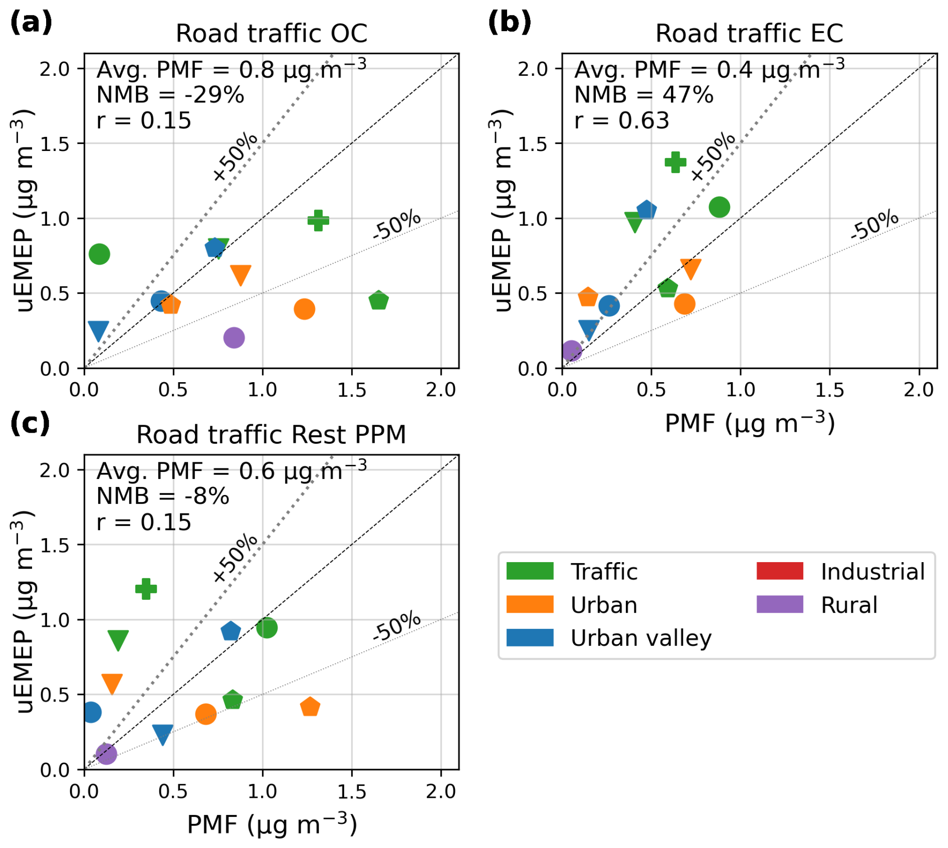
Figure 4 Average PMF-derived and uEMEP modelled road traffic OC (a), EC (b), and Rest-PPM (c) concentrations at the Weber et al. (2019) sites.

4.3.3 Station time series

Time series at the Grenoble Les Frênes (GRE-fr) station are shown to illustrate the temporal variations of the main PMF factors, being representative also of those derived at the other sites. Since the GRE-fr site does not identify the industrial and marine/HFO factors in the current dataset (the analysis of Ngoc Thuy Dinh et al. (2026); Borlaza et al. (2021) did identify an industrial factor at the Grenoble site), time series for these factors at the Port de Bouc (PdB) station are included in Fig. S4, to illustrate their overall low concentrations and high variability.

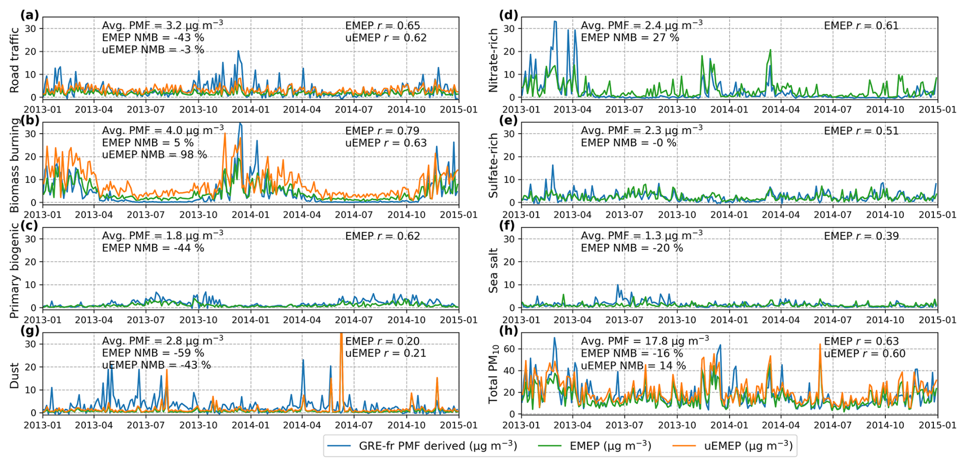
Figure 5 PMF-derived and modelled surface concentrations at the GRE-fr site between the years 2013 and 2014. uEMEP results are shown only for those factors affected by downscaling. Note the difference in y-axis scaling in panel (h).

Figure 5 shows the time series of the road transport, biomass burning, PBAP, dust, nitrate-rich, sulfate-rich, sea salt, and total PM₁₀ concentrations. Factors affected by downscaling show both the EMEP and uEMEP results whereas total PM₁₀ is calculated based on the combination of EMEP and uEMEP. Figure 5a shows that temporal variations of the road traffic factor are reasonably well described (r=0.62–0.65), although episodic wintertime peaks are underestimated. Downscaling with uEMEP further increases modelled concentrations throughout the year, leading to overestimations during the summer months. The latter compensates for the underestimated wintertime concentrations, resulting in an overall uEMEP bias of −3 %. For the biomass burning factor, wintertime peaks are underestimated to a lesser extent while its seasonal variations are more pronounced. The overall bias in uEMEP is high (98 %), with concentrations being overestimated already in the EMEP results.

Consistent with literature, PBAP PM has its highest concentrations during the summer months (Samaké et al., 2019a; Yttri et al., 2021). Its seasonal variations are well described, even though the model has a negative bias of −44 %. Seasonal variations of the nitrate-rich factor are limited to episodic events mostly during the cold period (October–March) while the sulfate-rich factor shows comparatively stable concentrations throughout the year. Sea salt also shows comparatively little variation, with concentrations being low. The dust factor shows episodic behaviour throughout the year, likely related to Saharan dust episodes. While such episodes are also present in the model, their timing and magnitude shows little overlap with the PMF results.

Total modelled PM₁₀ concentrations correlate reasonably well with the PMF results (r=0.60–0.63), with downscaling changing the model bias from −16 % to 14 %. Based on the individual PMF factor results, the uEMEP overestimation is largely result of the increase in biomass burning concentrations, overcompensating for underestimations in most other factors (an exception being the nitrate-rich factor). For reference, the model performance statistics for each of the factors at each of the Weber et al. (2019) sites is shown in Table S4.

5 Daellenbach et al. (2020b, 2017) PM₁₀ OA source apportionment and vehicular brake wear metals

Daellenbach et al. (2020b) combined PMF results for OA and vehicular wear metals with total aerosol oxidative potential (OP) measurements to derive source-specific (intrinsic) OP factors. The analysis was based on daily mean PM₁₀ quartz-fibre filter measurements from nine sites in Switzerland and Liechtenstein, being sampled every fourth day in the year 2013. The OA PMF results were based on those described in Daellenbach et al. (2017), using the offline Aerosol Mass Spectrometry (AMS) methodology described in Daellenbach et al. (2016). The latter employs mass spectral signatures (mass to charge ratios; $m/z$) for the identification of individual chemical compounds, with the bulk OA being removed from the filters based on water-extraction. For the purpose of deriving intrinsic OP values (and metal PMF factors), daily mean measurements from four sites (Bern, Magadino, Payerne, and Zurich) were aggregated into monthly and half-monthly bins in Daellenbach et al. (2020b), with trace metal contents (crustal material, metals) being determined using coupled plasma mass spectrometry. The trace element analysis identified PMF factors related to vehicular brake wear emissions (rich in Fe, Cu, Sb, Mo) and residential heating (Cd, Pb, Rb, Zn). However, since only the vehicular wear factor was implicated as a marker for aerosol toxicity (Daellenbach et al., 2020b), the residential heating metal-fraction is not discussed here.

The PMF analysis was performed using the ME-2 PMF engine with the Source Finder (SoFi) toolkit (Canonaco et al., 2013), distinguishing between primary and secondary OA using chemical fingerprints characteristic of SOA. POA was decomposed into its hydrocarbon-like OA (HOA), cooking OA (COA), sulphur-containing OA (SCOA), and biomass burning OA (BBOA) contributions. The COA factor was identified based in part on its correlation with fatty acids (Crippa et al., 2013a), being produced in the process of meat charbroiling. While food processing emissions are likely to be under-represented in the EMEP emission inventory (as is commonly the case, see Ots et al., 2016), cooking emissions from fuel use are included as part of GNFR C. For consistency with the modelled emission source, COA is combined with the BBOA factor (discussed in the following) to create a single factor representing fuel combustion from residential sources. This constructed factor is still referred to as BBOA, as biomass burning nevertheless dominates total GNFR C emissions. For example, biomass burning represents 99 % and 92 % of GNFR C emissions in France and Switzerland, respectively. In the PMF results, COA on average represents a contribution of 0.5 µg m⁻³.

As described in detail by Daellenbach et al. (2017), overall uncertainty estimates (err_tot) of the organic PMF factors depends on the derived factor concentrations. The ratio between err_tot and total concentrations (err_tot $/$ conc) can be as high as 2–4 when individual factor concentrations fall below 0.2 µg m⁻³. For concentrations above 0.5 µg m⁻³, and not considering the SCOA factor, the err_tot $/$ conc ratio is typically around 0.5. Uncertainties are generally lower for aSOA, having an err_tot $/$ conc ratio of around 0.2-0.3 for concentrations greater than 0.5 µg m⁻³. Uncertainties are highest for the SCOA factor, having an err_tot $/$ conc ratio of around 0.8 for concentrations of 0.5 µg m⁻³, in part due to a lack of factor specific chemical constraints and for being calculated as a mass closure term. For the SCOA factor, and to an extent also HOA, the uncertainty is further relatively high given the uncertain water-solubility. For average concentrations across all sites, uncertainties fall within the range of 0.20–0.32 µg m⁻³ for all OA factors (Daellenbach et al., 2017, Table 3), representing a typical uncertainty of around 20 %–30 %. Bootstrap runs and rotational ambiguity tests further found overall low uncertainties for the vehicular wear factor, having an IQR to median concentration ratio of around 0.1 (Daellenbach et al., 2020b).

5.1 PMF factors

Similar to the structure of Sect. 4.2, descriptions of the relevant PMF factors are given in the following along with a description of the modelled PMF factors and their matching to model output species. An overview of the matching to modelled species is also given in Table S5.

5.1.1 HOA, SCOA, and brake wear metals

The HOA, SCOA, and brake wear PMF factors all relate to vehicular traffic emissions. The HOA factor is associated with POA from vehicular exhausts and other liquid fossil fuel combustion sources, with a mean derived f_OA:OC of 1.32 and an IQR of 1.30–1.33 (Daellenbach et al., 2017). The mean f_OA:OC is in close agreement with the ratio of 1.25 assumed in the EMEP model. The HOA factor was included in the PMF analysis based on chemical profile spectra from Crippa et al. (2013b), being identified in part based on its association with diurnal traffic-induced variations. NO_x was used as a marker to constrain the PMF solution for HOA. In the EMEP model, HOA is calculated as POA from on-road and offroad vehicular exhaust emissions. Following Daellenbach et al. (2020b), POA from shipping emissions is also assigned to the HOA factor. While Daellenbach et al. (2020b) additionally assigned POA from industry and public power, the emission datasets employed in the current work are unable to distinguish between their respective liquid and solid fuel fractions. However, the underlying chemical speciation data reveals that OA from these latter emission sources is limited, representing less than 1 % and 10 % of their total PM_co and PM_2.5 emissions, respectively.

The PMF-derived SCOA was found to correlate with NO_x, in line with sulphur-containing emissions from vehicular tyre wear. The modelled SCOA factor is calculated as the OA fraction from on-road tyre wear, representing around half of the total modelled tyre wear PM mass. The vehicular wear PMF factor represents metals from break wear (Fe, Cu, Zn, Mb), with its PMF-derived mass contributions being dominated by Cu (4.51 %) and Fe (92.51 %). Modelled Fe and Cu concentrations are based on on-road vehicular brake wear emission data, with Fe and Cu together assumed to comprise 70 % of total brake wear PM mass (Hagino et al., 2024).

5.1.2 BBOA

The BBOA factor is associated with biomass (wood) burning emissions, being calculated as an unconstrained PMF factor using carbon monoxide (CO) as a marker. The resulting chemical profile is characterized by oxygenated fragments from anhydrous sugars such as levoglucosan. The mean measured f_OA:OC of 1.74 (Daellenbach et al., 2017) closely matches the ratio of 1.7 assumed by the EMEP model. Given the spatio-temporal correlation with other sources of residential combustion, POA from residential coal combustion can also contribute to this factor (Daellenbach et al., 2020b). In the model, all POA from GNFR C is assigned to the BBOA factor, in addition to POA from forest fires. As for the biomass burning PMF factor from Weber et al. (2019), forest fire contributions to the modelled BBOA factor are small (0.1 µg m⁻³ on average).

5.1.3 aSOA and bSOA

The aSOA and bSOA factors, sometimes referred to as winter oxygenated OA (WOOA) and summer oxygenated OA (SOOA), respectively, were identified based on their high contributions from oxygenated ions and their distinct seasonal variations (Daellenbach et al., 2017). bSOA was found to correlate well with temperature while aSOA was found to correlate with ${\mathrm{NH}}_{\mathrm{4}}^{+}$, the latter being associated with (long-range transported) SIA. The bSOA mass spectral signature was found to be similar to those reported for chamber SOA generated from terpene oxidation. For aSOA, the chemical profile was found to be characteristic of highly oxidized SOA from anthropogenic precursors (mostly from wood combustion Daellenbach et al., 2020b, 2019). Average f_OA:OC values were found to be 1.89 and 2.12 for bSOA and aSOA, respectively, with the ratio for aSOA being characteristic of highly aged OOA (Daellenbach et al., 2017). The f_OA:OC of 2.0 assumed by the EMEP model for aSOA, bSOA and background OA is in reasonable agreement with the PMF-derived estimates. All modelled aSOA and bSOA is assigned to the respective PMF factors. In addition, the background OA species is assigned to the bSOA factor, being representative of highly oxidized SOA from missing biogenic precursor emissions (Sect. 4.2.5).

Daellenbach et al. (2017) further note that the bSOA factor may contain OA from unresolved PBAPs, with the latter having similar seasonal characteristics. With the assumption that the derived bSOA factor is a linear combination of PBAPs and bSOA, and using the relative contribution of the ${\mathrm{C}}_{\mathrm{2}}{\mathrm{H}}_{\mathrm{5}}{\mathrm{O}}_{\mathrm{2}}^{+}$ ion (a marker of PBAP) to the derived bSOA profile, Daellenbach et al. (2017) roughly estimate that 17 % of bSOA may in fact be PBAPs, amounting to an average warm-season PBAP contribution of 0.30 µg m⁻³. Analysis based on co-located free cellulose measurements yielded an average warm-season PBAP estimate of 0.69 µg m⁻³. However, these aforementioned estimates were found to be about a factor of 3 to 10 lower than those reported by Bozzetti et al. (2016), indicating that the estimates are highly uncertain. Given the uncertainties involved in the PBAP contribution to the PMF-derived bSOA factor, and given that modelled PBAPs represent a significant source of OA (1.0 µg m⁻³ on average), all modelled PBAPs are added to the bSOA factor in part to avoid neglecting a significant source of OA mass.

5.2 Results

5.2.1 Annual mean concentrations

This section focuses on the results for PMF factors affected by downscaling at the four sites considered in Daellenbach et al. (2020b), where the vehicular wear factor is based on monthly and half-monthly averages. For the BBOA and HOA factors, results are based on all available 3-daily data from Daellenbach et al. (2017).

Figure6 shows the annual mean PMF and modelled concentrations for the HOA, vehicular wear, and BBOA factors, including the modelled local and non-local (i.e., outside of an approximately 30 km radius) contributions. These results indicate that HOA is underestimated by a factor of 2–8, with also the rural stations (Magadino, Payerne) showing considerably higher PMF-derived concentrations. The vehicular wear factor is better captured. The BBOA factor is overestimated by a large margin already in the EMEP model, which is exacerbated by downscaling with uEMEP. The overestimated BBOA concentrations at the Zurich and Bern sites are especially striking, with uEMEP concentrations of 7.6 and 4.9 µg m⁻³ being far removed from the PMF derived results of 0.5 and 0.7 µg m⁻³, respectively. For the urban sites (Bern and Zurich), local contributions dominate over those of the regional background. While not explicitly shown, both the PMF and model results for the vehicular wear factor show little seasonal variations.

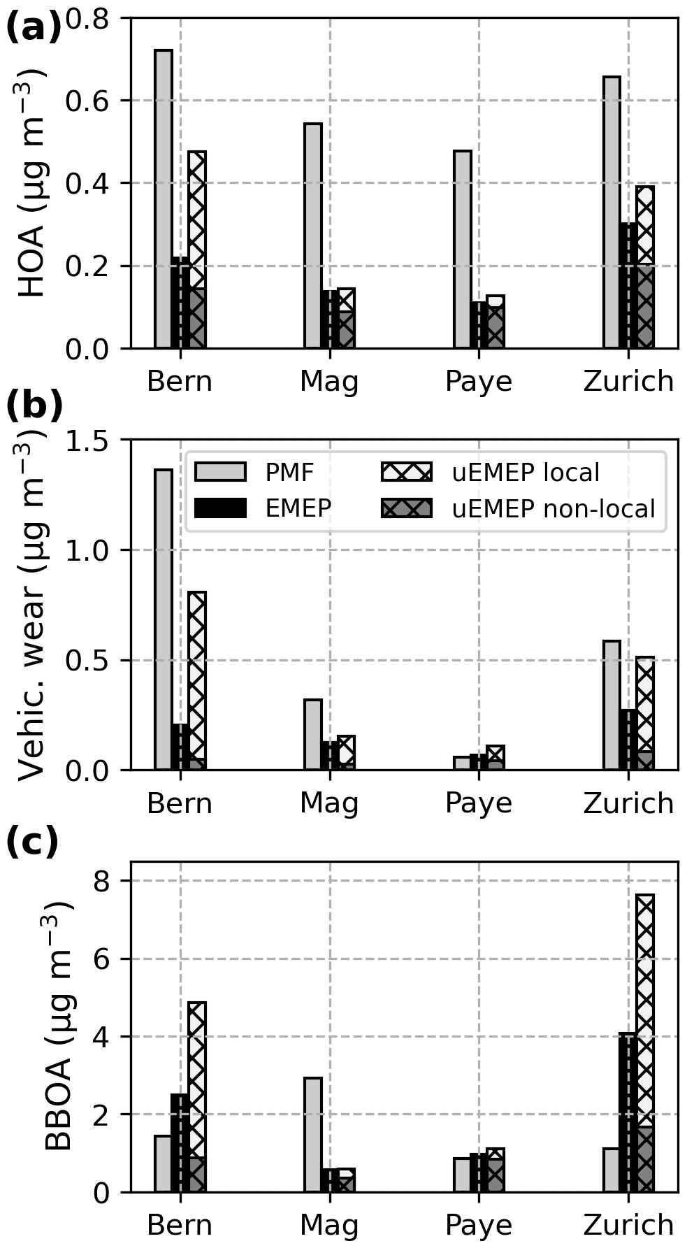
Figure 6 Annual mean PMF-derived and modelled HOA, vehicular wear, and BBOA concentrations for the year 2013 at four Swiss stations. Values calculated using uEMEP are split between their local and non-local contributions.

5.2.2 Daily mean data

Figure 7 shows daily mean time series the PMF-derived OA factors for the other five stations of Daellenbach et al. (2017), with results for the four stations from Daellenbach et al. (2020b) being shown in Fig. S5. For factors affected by downscaling, only uEMEP concentrations are shown. Figure 7 illustrates that the model describes the bSOA factor well, even though concentrations are overestimated in winter. Here the contributions from PBAPs are highlighted using shaded areas, illustrating that PBAPs contribute significantly to the modelled bSOA concentrations. aSOA peaks between January-April, and is in general underestimated by a large margin. The HOA factor shows elevated concentrations during the cold period while also being underestimated by the model. BBOA is overestimated by a large margin at all sites except Vittore, where it is instead underestimated by around a factor of ten. The SCOA factor shows generally large underestimations and poor correlations. While the modelled HOA and SCOA factors are closely related based on their relation to modelled road traffic PPM, the correlation between the PMF-derived HOA and SCOA factors is poor (r<0.32). For all station and PMF factor combinations from the Daellenbach et al. (2020b, 2017) dataset, model statistics are shown in Table S6 for both the EMEP and uEMEP models. In addition, scatter plots of the OA PMF factors from all stations are shown in Fig. S6. Including any unassigned sources of OA in the model further increases average modelled total OA concentrations by 0.1 µg m⁻³, indicating that effectively all OA mass is accounted for in the analysis.

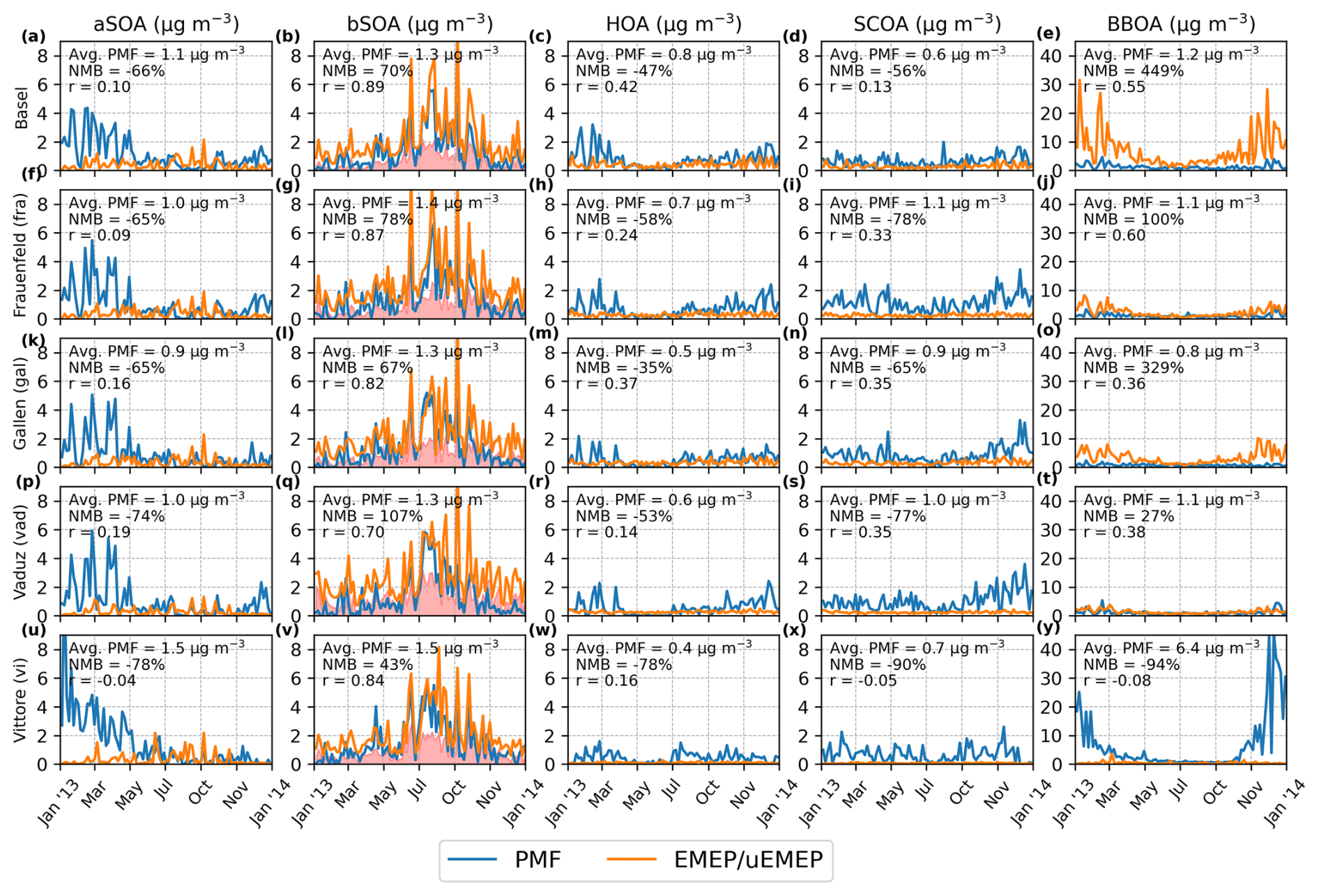
Figure 7 Comparison of the PMF-derived OA fractions from Daellenbach et al. (2017) and the corresponding EMEP/uEMEP modelling results. Note the difference in y-axis scaling for the right-hand panels. Shading in the panels showing bSOA indicate the modelled contribution of PBAPs to this factor.

6 Chen et al. (2022) PM₁ OA source apportionment

The Chen et al. (2022) dataset is comprised of PMF-derived PM₁ OA source apportionment based on Atmospheric Chemical Speciation Monitor (ACSM) measurements obtained at 22 sites. In the current work, data from the 9 sites located within the modelling domain of Fig. 1 are used. ACSMs operate by accelerating aerosol passing through an inlet, impacting it on on a vaporiser (600 °C), and ionising the resulting vapours. The ionized vapours are then analysed using a mass spectrometer to determine their $m/z$ ratios, relating to the chemical structure of organic and inorganic molecules contained within the aerosol. Chemical fingerprints based on these measurements are used as input to the PMF analysis.

Contributions from HOA, BBOA, COA, and oxygenated organic aerosol (OOA) were determined using a rolling PMF technique employing a time-window between 7 to 28 d, following the standardized 5-step protocol described in Chen (2022). Using the rolling PMF technique, factors are estimated based in part on their daily and seasonal time-variations, adjusting their chemical profiles according to their seasonal characteristics (Canonaco et al., 2021; Chen et al., 2021). Liquid fuel and wood burning fractions of equivalent black carbon (eBC) were used as markers for the HOA and BBOA factors, respectively, as determined from co-located filter-based absorption photometer measurements. For the stations in the current work, HOA factor profiles were based on Crippa et al. (2013a) and on station-specific wintertime measurement data. The BBOA profiles were based on either Ng et al. (2011), Fröhlich et al. (2015), station-specific wintertime data, or the solution obtained from its inclusion as an unconstrained factor. Rotational and statistical uncertainty were estimated following the approach outlined in Canonaco et al. (2021), with the average PMF uncertainty amounting to 20 % and 23 % for the HOA and BBOA factors, respectively. As for the Daellenbach et al. (2017) dataset, COA results are added to the BBOA factor for consistency with the modelled GNFR C emission sector. On average, COA concentrations amount to 0.2 µg m⁻³ at the Chen (2022) sites discussed in this work. The PMF analysis further identified a combined shipping and industry OA factor at the Marseilles site, a “58-OA” factor at the Magadino site, and cigarette smoke OA (CSOA) at the Zurich site. Since these factors represent relatively small mass contributions (4 %, 2 %, and 16 % to PM₁ OA at the respective sites), these are not considered here. These factors represent a combined average contribution of less than 0.1 µg m⁻³ to the results discussed in this work.

The HOA and BBOA factors from Chen et al. (2022) are taken to be comparable to those described for the Daellenbach et al. (2017) dataset, even though there are underlying differences in their PMF methodologies and measurement techniques. However, Chen et al. (2022) does not distinguish between the aSOA and bSOA factors, instead deriving a more oxidised-oxygenated OA (MO-OOA) and less oxidised-oxygenated OA (LO-OOA) factor. Since the default EMEP model does not distinguish between MO-OOA and LO-OOA, these factors are combined into a single OOA factor. This factor is taken to be a proxy for all secondary organic aerosol (i.e., aSOA and bSOA), with total OOA having an average uncertainty of 22 % (Chen, 2022). Furthermore, the PBAPs included in the Daellenbach et al. (2017) bSOA factor are exclusively modelled in the coarse aerosol fraction, and are therefore not included in the modelled OOA factor here. For HOA and BBOA, the large majority of mass is in general contained within the PM₁ fraction (e.g., Luo et al., 2022). Diagnostic analysis where the coarse aerosol fractions are excluded from the modelled Daellenbach et al. (2020b) factors are indeed found to differ by no more than 0.001 µg m⁻³ relative to the PM₁₀ results. SOA is by its nature contained mainly within the PM₁ fraction (Pandis et al., 1993). While the ACSM data is provided at 30 min intervals, the data is aggregated into hourly and daily means for the purpose of comparing to the EMEP and uEMEP model results. An overview of the matching between modelled species and the Chen (2022) PMF factors is given in Table S7.

6.1 Results

6.1.1 Station average concentrations

Figure 8 shows the average PMF-derived and modelled concentrations at the nine Chen et al. (2022) sites. Here all data has been aggregated into daily means for consistency with the previously described datasets. Figure 8 shows that the HOA factor is changed very little by uEMEP downscaling, indicating that the stations are not located near to roads. The BBOA factor is severely overestimated by the EMEP model, with downscaling increasing the positive biases at urban sites, even though downscaling has an overall modest impact. Overestimated BBOA concentrations are most severe at the Zurich site (consistent with the results from the Daellenbach et al. (2017) dataset), amounting to 8.7 µg m⁻³ in uEMEP versus 0.2 µg m⁻³ from the rolling PMF analysis. Omitting this station changes the overall model NMB from 192 % to 105 % and the correlation coefficient from −0.21 to 0.11. The OOA factor is further underestimated by around a factor of two while showing a slightly negative correlation.

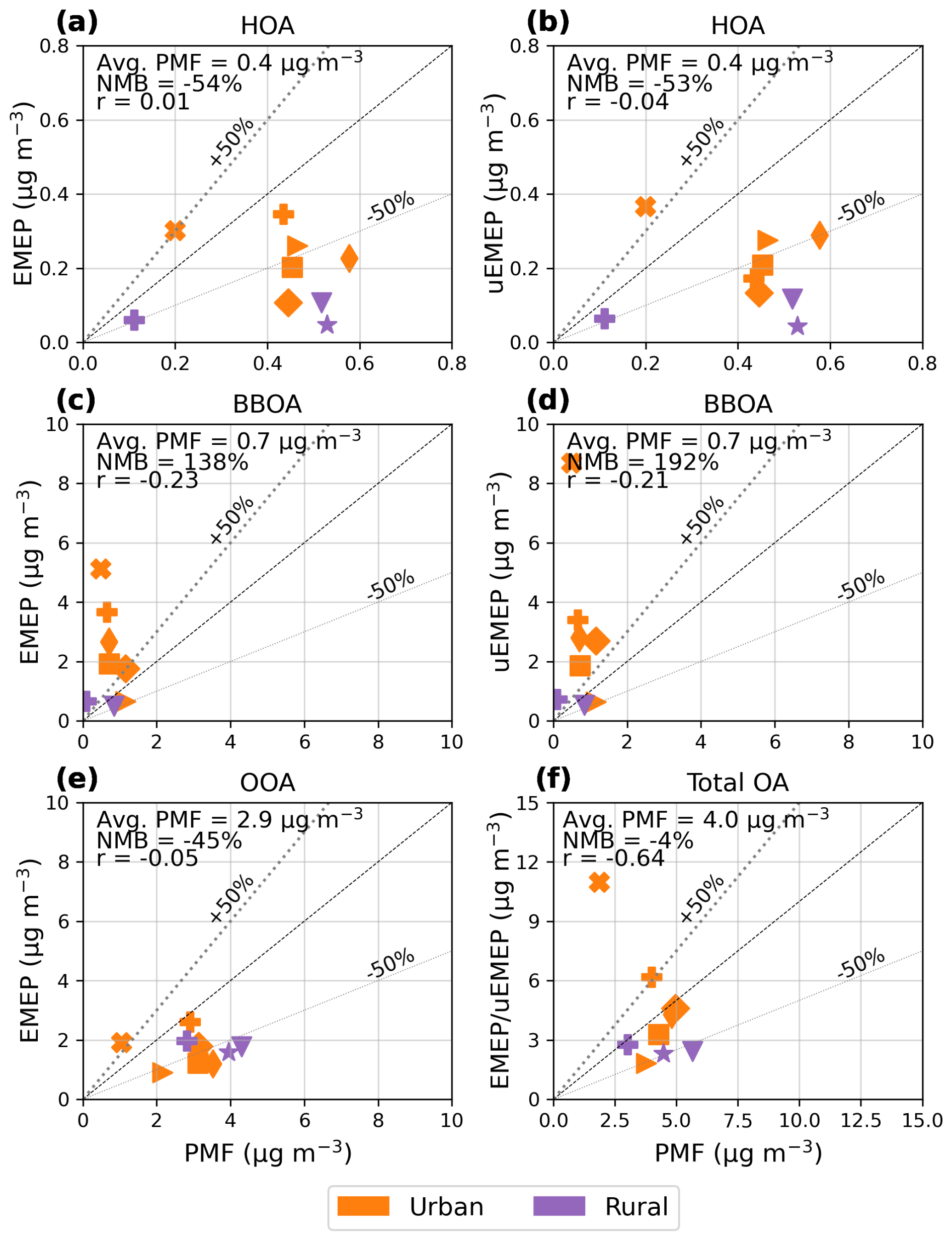
Figure 8 Average observed and simulated PMF factor concentrations at the Chen et al. (2022) sites. Markers correspond to those shown in Fig. 1. Note the differences in axis scaling between the panels.

For all three factors, and for both the EMEP and uEMEP models, the correlation between the PMF and modelled concentrations is in general poor. Furthermore, in the PMF results the majority of OA mass is contained within the OOA factor, indicating that the stations are comparatively far removed from primary sources. In the model, however, the primary BBOA factor dominates OA mass. For total OA concentrations calculated based on the individual PMF factors (Fig. 8f), the model bias is low while also showing a large negative correlation. As for the Daellenbach et al. (2017) dataset, any unaccounted for (i.e., unassigned to modelled PMF factors) sources of modelled OA amount to 0.1 µg m⁻³ on average, illustrating that effectively all modelled PM₁ OA is accounted for by the modelled PMF factors.

6.1.2 Station time series

Time variations of the Chen et al. (2022) PMF factors are illustrated using the results from the Paris site, with time series of the HOA, BBOA, and OOA factors being shown in the left-hand panels of Fig. 9. Daily averages are shown here to match the time series analysis of the Weber et al. (2019) and Daellenbach et al. (2017) datasets. However, the middle and right-hand panels of Fig. 9 show average diurnal variations based on the underlying hourly data for the cold period and warm period.

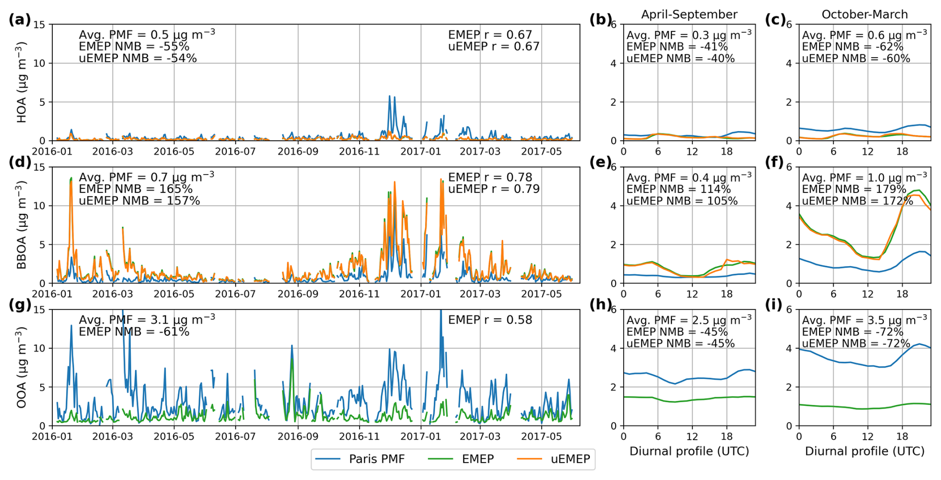
Figure 9 PMF-derived and modelled surface concentrations at the Paris site based on daily average results (a, d, g) and hourly results (other panels). uEMEP results are shown only for factors affected by downscaling.

Figure 9a-c illustrate that, consistent with the results of Fig. 8, HOA is largely underestimated while downscaling also has very little effect. Underestimations are particularly severe during the winter months, when PMF concentrations can reach values up of to 6 µg m⁻³. While the model captures the timing of peak concentrations reasonably well, having an overall correlation coefficient of 0.68, their magnitude is severely underestimated. Daily maximum concentrations further occur around 21:00 UTC in both the warm and cold periods, whereas modelled concentrations peak around 16:00 and 06:00 UTC during these respective time periods (although HOA concentrations are generally low).

Figure 9d-f demonstrates that BBOA temporal variations are captured well by both the uEMEP and EMEP models, even though average concentrations are underestimated. The diurnal variations are also well described, although here modelled concentrations peak around 1–2 h (21:00–22:00 UTC) earlier than those derived from the PMF analysis. The OOA factor displays high episodic concentrations throughout the year, with its concentrations being highest during the cold period. Modelled OOA concentrations are underestimated especially during the cold period. Notable is that for the BBOA factor at the Zurich site, the large model overestimation is similar to that found for the Daellenbach et al. (2020b) dataset, with average EMEP and uEMEP modelled concentrations of 5.3 and 8.9 µg m⁻³, respectively, compared to a PMF-derived average of 0.2 µg m⁻³. For reference, the NMB and correlation statistics for each of the seven sites from the Chen et al. (2022) dataset are shown in Table S8. Table S9 in addition shows the station statistics based on hourly mean data, although these are not notably different to the daily average results.

7 Discussion

Table 2 summarizes the model performance based on all available station data from the datasets discussed in the previous sections. As before, the Pearson correlation statistic is calculated based on station average data to reflect the model skill in reproducing site-to-site variability (spatial correlation). However, the correlation between modelled and PMF-derived time series at individual sites is a measure of the model skill in capturing temporal variations (denoted r_t). Table 2 thereby also shows the average r_t based on the values calculated at each of the sites. Furthermore, for the Chen (2022) dataset, the model results at the Zurich site for POA from residential wood combustion (BBOA) as well as total OA represent clear outliers (with results being overall more variable for the BBOA factor at the Daellenbach et al. (2017) sites). In Table. 2, the Zurich site is therefore omitted in the statistical analysis of the Chen (2022) PMF results.

Table 2 Statistics based on daily mean data from all PMF datasets described in Sect. 4–6. The OOA^* factor is constructed as the sum of the aSOA and bSOA factors.

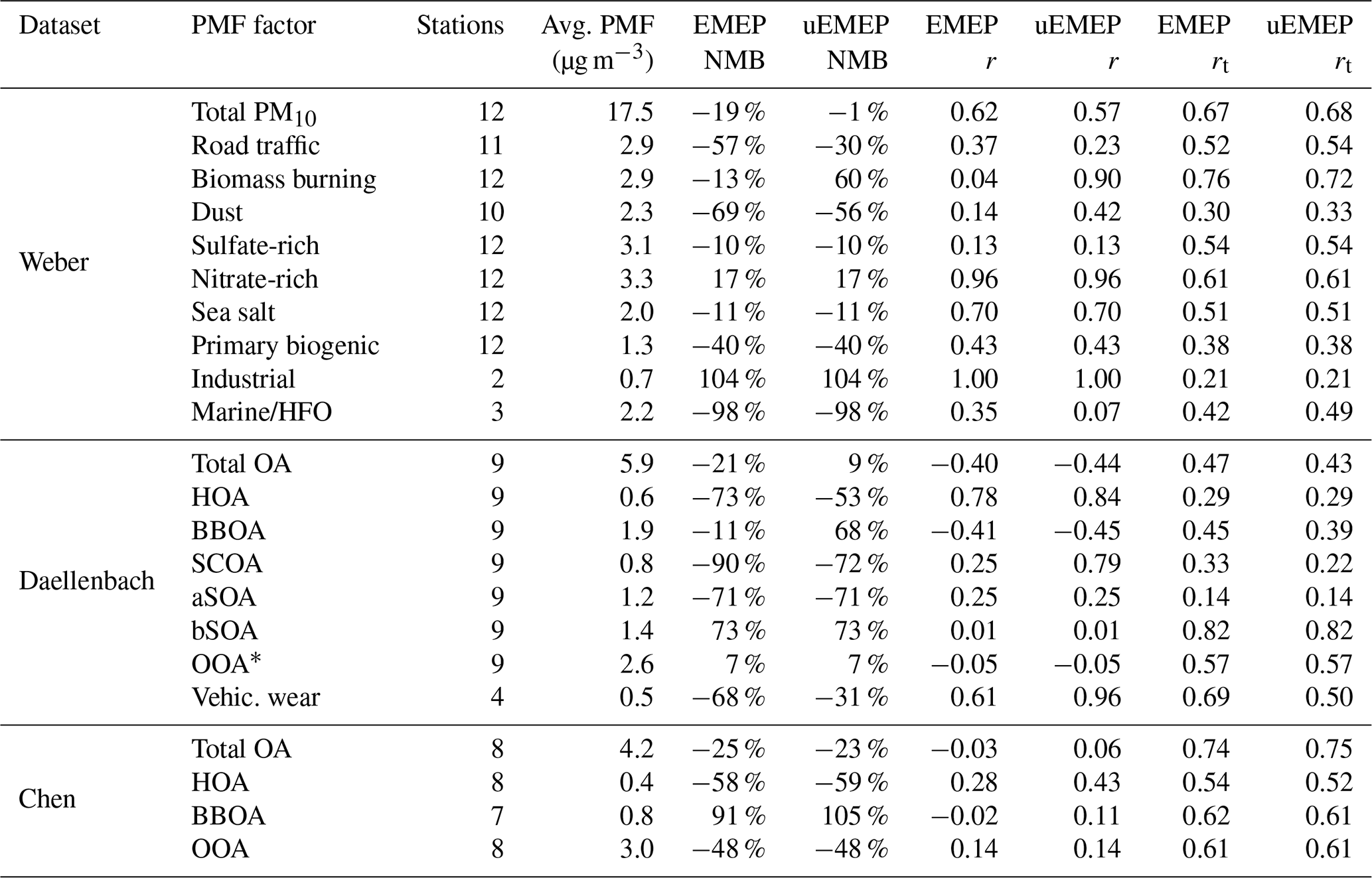
These results highlight that the model performance for PMF factors related to vehicular emissions (road traffic, HOA, SCOA, vehicular wear) is poor across the datasets, even though downscaling reduces their negative biases. The vehicular factors are nevertheless underestimated by 30 %–70 % even after downscaling. While the spatial correlations for the Daellenbach et al. (2020b, 2017) HOA, SCOA, and vehicular wear (brake wear metal) PMF factors are good, their temporal correlations are poor (r_t≤0.50). For HOA, and OA in general, one reason for the model discrepancies may be that the measured composition of OA and f_OA:OC can vary considerably by location, season, and time of day, for example due to differences in sources and combustion efficiencies (Font et al., 2024). However, while such variations may affect the spatial and temporal correlation scores, the average PMF-derived f_OA:OC ratios were nevertheless found to be in good agreement with those assumed in the EMEP model. For the modelled vehicular wear and SCOA factors, their contributions represent only small fractions of total modelled road traffic PPM (GNFR F). For these factors, small changes in the model assumptions (e.g., for the metal content of vehicular brake wear) and the GNFR F sub-sector emission inventories may therefore have a comparatively large impact on the results, given that their PMF-derived concentrations are also low.

The difference in average PMF-derived HOA concentrations between the Daellenbach et al. (2017) and Chen et al. (2022) factors could be the result from the large site-to-site variability in combination with the limited number of sites. However, uncertainties in the PMF analysis and underlying measurement techniques may also play a role, given that HOA concentrations are low. Table 2 further shows total OOA concentrations derived from the (offline) Daellenbach et al. (2017) and (online) Chen (2022) datasets, with average concentrations from the latter being higher, possibly due to higher OOA concentrations derived using the rolling PMF technique compared to the offline analysis (Chen et al., 2021). The EMEP model shows a small positive bias for the total Daellenbach et al. (2017) OOA whereas OOA from Chen (2022) is underestimated by a considerable margin (−48 %). The better bias performance for the former may relate to the modelled PBAP assigned to the Daellenbach et al. (2017) bSOA factor, which contributes 1.0 µg m⁻³ on average.

The model performance for many of the Weber et al. (2019) factors is encouraging. However, the bias and error in spatio-temporal variations in factors such as dust and biomass burning goes beyond what may be expected from the statistical PMF error. The model performance is especially poor for the industrial and marine/HFO factors, although these are based on a limited number of sites. In contrast, results for the sulfate-rich, nitrate-rich and sea salt factors are overall good. The latter factors also make relatively large contributions towards total PM₁₀ mass, with the model skill in reproducing total PM₁₀ being consistent with earlier EMEP evaluations in France. For aSOA, the accuracy of its inclusion in the modelled factor(s) is also limited by its unclear identification in the PMF analysis. Similar challenges involved in the matching to the Weber et al. (2019) PMF factors are underlined by Pekel et al. (2025) and Vida et al. (2025), although an inter-comparison of model methodologies is challenging in part due to differences in the treatment of SOA and the use of different emission sector definitions.

7.1 Condensable wood burning emissions

Biomass burning makes an important contribution to total PM₁₀ and OA mass, in line with nearly all stations being classified as either urban or traffic sites in urban areas. This makes accurate modelling of its mass contribution especially important, whereas Table 2 indicates that the factors relating to biomass burning are overestimated by 60 %–105 % after downscaling. One possible reason for this is the default treatment of condensable primary organic aerosol (CPOA) in the model. As described in detail in Donahue et al. (2006) and Robinson et al. (2010, 2007), the CPOA fraction of biomass burning aerosol is comprised of low-volatility SVOCs from wood burning emissions. These SVOCs quickly condense to form particulate matter upon emission into the atmosphere. However, as the emission plume dilutes, partial vapour pressures and primary condensation surface area concentrations are reduced, leading to the re-evaporation of the semi-volatile compounds. For example, going from an atmospheric dilution ratio of 20 to 120 can reduce particulate OC from wood burning by 75 % (Lipsky and Robinson, 2006). The resulting gaseous SVOC fraction can in turn efficiently age (oxidize) to form SOA over the course of a few hours, owing to their comparatively low volatility (Grieshop et al., 2009).

The GNFR C emissions included by default in the EMEP model are based upon emission factors derived from dilution tunnel (DT) experiments (Denier van der Gon et al., 2015a), being representative of the PM emissions as the smoke leaves the smoke stack. In the default treatment, CPOA is assumed to be non-volatile (i.e., all counted towards PPM). This representation was deemed appropriate for the typical grid-box size of the EMEP model (approximately 10 km by 10 km), and has been shown to give comparable results to the use of more elaborate schemes involving volatility basis set (VBS) approaches (Robinson et al., 2007; Simpson et al., 2012, 2022). Given the EMEP model's primary aim of support to policy making, it is also important to avoid arbitrary assumptions (e.g., addition of semi- and intermediate- volatility compounds) that are inconsistent with officially reported emissions. However, the non-volatile CPOA assumption is likely poor for urban-scale modelling. This is illustrated with diagnostic analysis of the weighted mean travel time for the downscaled (local) GNFR C PM using the uEMEP model, as shown for the year 2016 in Fig. S7. The latter indicates that travel times towards the measurement sites are typically between 10–20 min, and at most 48 min.

One solution would be to reduce the downscaled fraction of residential wood burning primary OC emissions, under the assumption that the SOA derived from volatile CPOA precursors is formed on EMEP rather than uEMEP spatio-temporal scales. As a conservative estimate of the 50 %–80 % fraction of the traditionally defined POA that exists in vapour phase at atmospheric conditions (Grieshop et al., 2009), this reduction factor can be chosen to be a factor of two (equivalent to a volatile CPOA ratio of 0.5). SOA derived from CPOA precursors can then also be counted towards the aSOA and OOA PMF factors, given that they are derived from the oxidation of precursor species. That a part of what is considered as non-volatile PM in the emission inventory should be assigned to OOA species, is further supported by the sum of the PMF-derived aSOA and BBOA factors showing overall better agreement with the default modelled BBOA factor (Fig. S8).

7.1.1 Impact on simulation results

As shown in Table 3, applying a volatile CPOA ratio of 0.5 reduces the overall bias of the downscaled Weber et al. (2019) biomass burning factor from 60 % to 29 %, being the result of the change in its modelled OC fraction (from 2.3 to 1.8 µg m⁻³, compared to a PMF-derived average of 1.4 µg m⁻³). Note that for the biomass burning factor, primary and secondary OA from wood burning is assumed to be contained within this single PMF factor, such that a distinction between primary and secondary OA does not apply here. Although the mean PMF-derived f_OA:OC of 1.7 can be considered low for a factor that is a mix of primary and secondary biomass burning OA, given that it is similar to the f_OA:OC derived for the (primary) BBOA factor by Daellenbach et al. (2017). While the overall bias in PM₁₀ changes from −1 % to −6 %, this is in line with most other PMF factors being underestimated. The overall correlation statistics are affected by no more than 0.03 for both the biomass burning and total PM₁₀ results.

Table 3 As Table 2 but now comparing model configurations where a volatile CPOA ratio of 0.5 is assumed (indicated by EMEP^* and uEMEP^*). Only PMF factor relevant to biomass burning are shown.

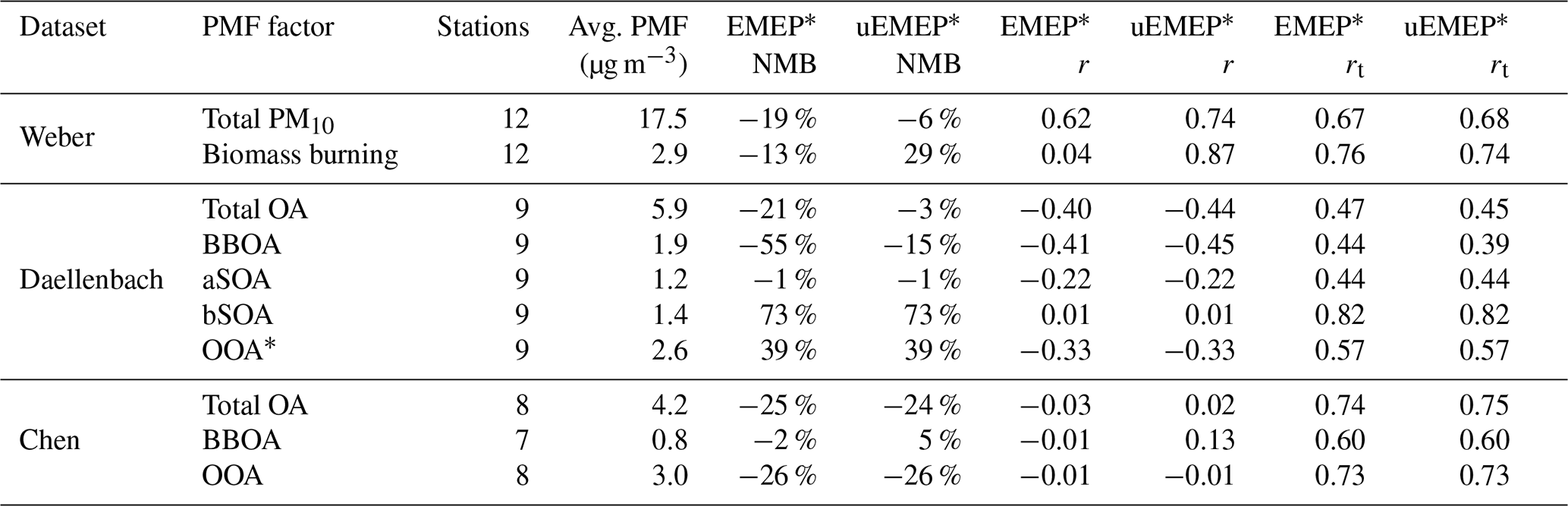
Assigning the volatile CPOA fraction to the aSOA and OOA PMF factors considerably increases the model skill for these factors, even though (spatial) correlations remain largely unchanged. Temporal variations at the individual sites (both rural and urban) are largely unchanged for the BBOA factor, while they are considerably increased for the aSOA factor. Temporal correlations for the OOA factor are impacted to a lesser extent, given the already present influence of bSOA. Applying the CPOA fraction largely removes the large positive bias in the modelled BBOA factors. However, it remains unclear to what extent SOA derived from the oxidation of semi-volatile precursors contributes towards the oxygenated OA factors, and to what extent these factors may be influenced by aged POA. For example, ageing of POA can lead to the production of OOA also in the absence of sunlight (Kodros et al., 2020; Tiitta et al., 2016). Ageing of POA may also explain in part why the Chen (2022) OOA factor remains underestimated by −26 %, even after assigning the modelled volatile CPOA fraction. The assumption that the PMF-derived aSOA factor can be associated with the SOA formed by the rapid oxidation of low-volatility precursors also contrasts with the suggestion of Daellenbach et al. (2017) that aSOA represents highly aged OA. Furthermore, a clear link between the BBOA and aSOA factors is not always present in the PMF results. For example, at the Vittore station (Fig. 7u–y) BBOA concentrations are high from November onwards while aSOA concentrations are practically zero during this time, even though the BBOA and aSOA factors do vary concurrently between January and April.

The large site-to-site variability between modelled and PMF-derived biomass burning concentrations, for both urban and rural sites, can also be indicative of a poor representation of the spatial distribution in the EMEP emission inventory, and possibly also of the uEMEP downscaling proxy (population density). In particular, the results for the Vitorre, Magadino, Basel, and Zurich sites show vastly different results between the PMF-derived and modelled concentrations, going beyond the changes achieved by imposing the CPOA assumption. The location and magnitude of residential wood combustion (RWC) emissions in inventories is indeed known to be uncertain, being hampered for example by differences in wood burning regimes between different geographical regions (Daellenbach et al., 2018). The RWC modelling study of Denier van der Gon et al. (2015a) used a specialised spatial distribution for RWC emissions, and Ots et al. (2018) found better EMEP model results for the United Kingdom when RWC emissions were redistributed from urban to rural areas. For reference, a synthesis of the statistical results across datasets and PMF factors (following Table 2) with the CPOA assumption is given in Table S10.

8 Conclusion

By leveraging results from the three PMF source attribution datasets discussed in this work, common model strengths and weaknesses were identified. Model strengths include the ability to describe seasonal variations of individual PMF factor concentrations, for example related to biomass burning, while also showing favourable spatial (site-to-site) correlations for many other factors. However, the simulation of OA sources remains challenging across the datasets, with source-specific contributions from primary and secondary OA often being obscured (both in the PMF analysis and model emission inventories). The interpretation with respect to site-specific or highly process-bound PMF-factors also remains challenging, where multiple PMF factors have sometimes been combined into single factors to aid their inter-comparison with modelled quantities. Validating the model results is further challenged by PMF analysis itself being an inverse modelling technique, having its own inherent sources of known and unknown uncertainty. In this respect, a harmonized PMF protocol applied to both measured and modelled quantities would be beneficial (Chen et al., 2010), shedding light on how PM from co-varying model sources may be captured by individual PMF factors. The main findings and conclusions of the current work can be summarized as:

• For the datasets considered in the current work, the total aerosol mass quantities that the EMEP and uEMEP models have traditionally been compared to consistently perform well, even though spatial correlations for total OA are poor. For mass concentrations, arguably being the most important model evaluation metric for mass based health indicators, individual factor concentrations often show under and over-predictions beyond those which may be expected from the statistical PMF uncertainty. This suggests that at least some degree of compensation of errors may be taking place in the total mass calculations, with the PMF analysis revealing possible errors in the underlying modelled source contributions.

• PMF factors relating to residential heating and road traffic make comparatively large contributions towards total PM₁₀ and OA mass. Their modelled concentrations are further strongly impacted by urban downscaling using uEMEP, reducing the negative bias seen across factors relating to road traffic. However, downscaling can also enhance existing biases, with overall model skill for factors relating to road traffic and biomass burning remaining poor. The results further point towards possible errors in the spatial distribution of residential heating emissions, showing exceedingly large over and underestimations at a number of urban and rural sites.

• Model results related to biomass burning are considerably improved when a 50 % volatility assumption is applied to CPOA from residential wood burning. In this framework, volatile CPOA is excluded from downscaling with uEMEP while also being assigned to oxygenated rather than primary OA PMF factors. This simplified treatment of SOA principally serves to highlight the sensitivity of modelled BBOA and OOA to the treatment of CPOA, with more realistic implementations depending on photochemistry, ambient temperatures, and the availability of organic condensation surfaces (Donahue et al., 2006). Oxygenated OA factors may further also depend on the ageing of POA (Shrivastava et al., 2008), which is not included in the default version on the model as used here.

One of the overarching motivations behind the current work is the close relationship between PMF analysis and newly suggested measures of aerosol toxicity such as aerosol OP. Within current state-of-the-art OP frameworks, PMF-derived aerosol sources are assigned intrinsic OP values based on their (grouped) chemical characteristics, with total OP being calculated as a linear combination of its individual PMF factor contributions (Weber et al., 2021; Daellenbach et al., 2020b). The quality of total modelled OP is then to a large extent determined by the quality of the underlying PMF factor calculations, in particular for those factors having a high intrinsic OP (predominantly related to urban anthropogenic emission sources). Our results highlight that, at least within the framework of the EMEP/uEMEP modelling system, the most important intrinsic OP sources are also the most difficult to model. For example, in addition to the overall poor model skill in reproducing vehicular traffic PMF factors, the discussed distinction between primary and secondary OA from wood burning emissions also relates to a factor of five difference between their intrinsic OP values (Daellenbach et al., 2020b). Joint efforts must be pursued to establish a better matching between statistical regression models and CTMs so as to be able to simulate OP properly at an acceptable epidemiological scale.