Decomposing pre-industrial to present-day land use change forcing in the UK Earth System Model

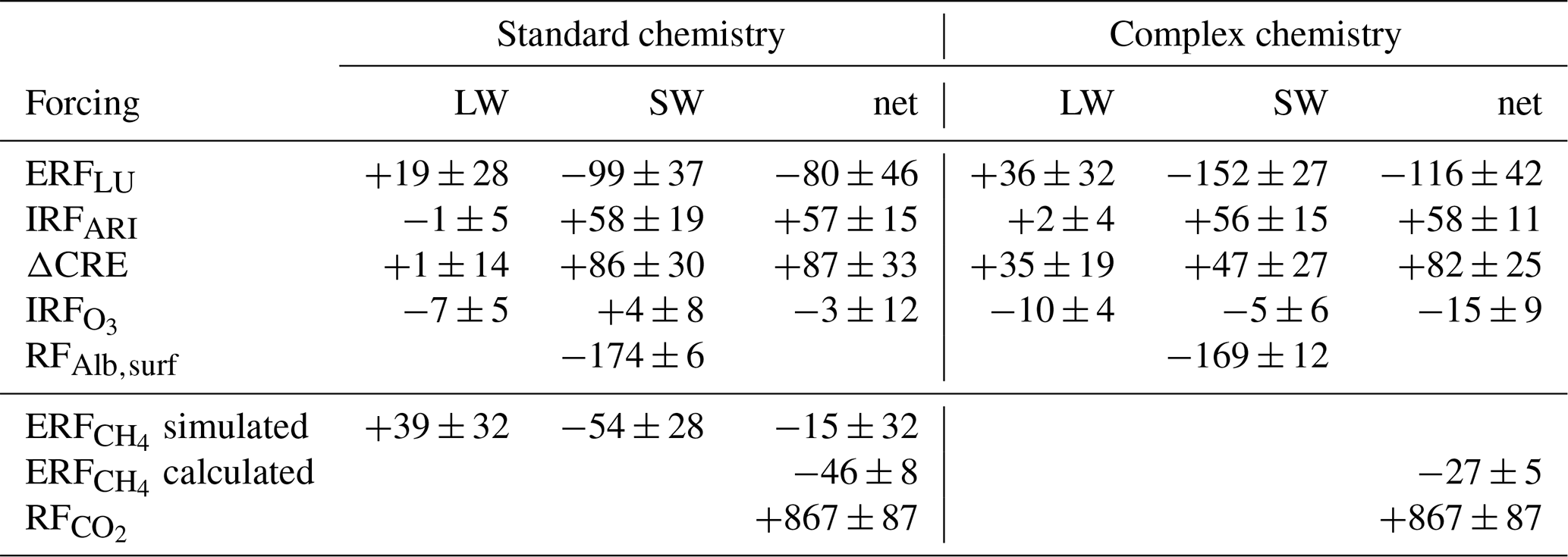
Land use impacts climate through changes in carbon emissions, surface albedo and evapotranspiration, as well as biogenic volatile organic compound (BVOC) emissions, which influence atmospheric composition. The relative importance of changes in atmospheric composition driven by pre-industrial to present-day land use change has not been assessed for the UK Earth System Model (UKESM). Here, we decompose the pre-industrial to present-day land use change forcing in UKESM1.1 with additional process updates. We find a net simulated forcing of $-\mathrm{0.08}\pm \mathrm{0.05}$ W m⁻² when using the standard (Strat-Trop vn1.0) chemistry, and $-\mathrm{0.12}\pm \mathrm{0.04}$ W m⁻² for a more complex (CRI-Strat 2) chemical mechanism. The simulated forcing includes the positive aerosol direct and indirect effects (around +0.06 and +0.085 W m⁻², respectively), alongside negative forcings from ozone (around −0.01 W m⁻²) and surface albedo change (around −0.17 W m⁻²). The forcing from the aerosol indirect effects calculated in this study is greater than in recent UKESM BVOC forcing experiments, which we attribute to using pre-industrial background conditions and increased organic matter hygroscopicity. Additional calculations show the radiative forcing from changes to methane lifetime is between −0.02 and −0.04 W m⁻², while the land use carbon emissions drive a carbon dioxide forcing of +0.87 W m⁻². Overall, the competing effects of changes in aerosols and short-lived greenhouse gases with surface albedo counter around 15 % of the carbon dioxide forcing. However, non-carbon dioxide effects have significant regional impacts, which reach −2.19 W m⁻² from surface albedo change in North America.

1 Introduction

Land use change is the source of around one-third of the total anthropogenic carbon dioxide (CO₂) emissions since 1750 (Canadell et al., 2007). Additionally, changes in land cover influence surface albedo, surface roughness and evapotranspiration (Davin et al., 2007; Davin and Noblet-Ducoudré, 2010), while the loss or gain of vegetation affects the emissions of various gases and aerosols (e.g. Ganzeveld et al., 2010; Ito and Hajima, 2020; Wu et al., 2012). Despite recognition that land-use driven changes in atmospheric composition have climate impacts (Fiore et al., 2012; Heald and Spracklen, 2015), only a few studies have attempted to decompose the pre-industrial (PI) to present-day (PD) radiative forcing from changes in land use/land cover, referred to here as land use, into the various atmospheric chemistry and aerosol pathways (Heald and Geddes, 2016; Scott et al., 2017; Unger, 2014a, b; Ward et al., 2014). Additionally, the continued development of Earth system models (ESMs) results in the inclusion of new and updated process representation that impacts these forcings (e.g. Weber et al., 2022). This study re-evaluates the PI to PD land use radiative forcing using the United Kingdom Earth System Model vn1.1 (UKESM1.1) with these updated or new processes and parameterisations, focusing on the changes in atmospheric chemistry and aerosols.

There are multiple pathways through which land use change can drive changes in atmospheric composition that have climate impacts. Biogenic volatile organic compounds (BVOCs) are tropospheric ozone (O₃) precursors, while their oxidation reactions can also be O₃ sinks. Consequently, any change in their emission can affect the concentrations of this greenhouse gas, although the sign of the impact will also depend on nitrogen oxide (NO_x) concentrations (Seinfeld and Pandis, 2016). In addition, BVOCs are rapidly oxidised in the troposphere and can, therefore, affect the availability of the hydroxyl radical (OH) for reactions with other gases, resulting in a link between BVOC emissions and the atmospheric oxidation capacity (Lelieveld et al., 2008; Wang et al., 2022). Of particular interest for the land use radiative forcing is the potential impact via OH on the methane (CH₄) lifetime. Finally, BVOCs are also secondary organic aerosol (SOA) precursors and, consequently, affect both aerosol-radiation interactions (ARI, also known as the aerosol direct effect) and aerosol-cloud interactions (ACI, or the aerosol indirect effects), thereby influencing climate (e.g. Scott et al., 2014).

The influence of NO_x on O₃ formation is just one example of how the impacts of changes in BVOC emissions depend on background conditions. The BVOC emission flux is sensitive to atmospheric CO₂, as well as temperature and sunlight (Guenther et al., 1995, 2012; Hantson et al., 2017). The initial availability of oxidants will determine how important a land-use driven change in BVOCs is for, e.g., aerosol formation pathways and methane lifetime. Previous studies have found that PI to PD aerosol forcing calculations are significantly affected by the background aerosol state in the PI (Carslaw et al., 2017; Rap et al., 2013). Further, the geophysical effects of land use change, such as changes in albedo and evapotranspiration, affect the radiative balance and drive rapid adjustments (e.g. changes in surface temperature) that can feedback on biogenic emissions.

Previous research into PI-PD land use radiative forcing from changes in atmospheric composition has used a variety of models and experimental set ups, as well as definitions of radiative forcing, leading to a wide range of results. The effective radiative forcing (ERF) is the change in the top-of-atmosphere net radiative flux (incoming − outgoing) after tropospheric and stratospheric adjustments, while Earth's surface temperature remains fixed. Ideally, both land surface and ocean temperatures would remain fixed. However, due to modelling constraints, land surface temperature adjustments are typically allowed to occur. Alternative metrics include the stratospherically-adjusted radiative forcing (SARF), which focuses on the change in the radiative flux after allowing for stratospheric adjustments but keeping the tropospheric conditions fixed, and the instantaneous radiative forcing (IRF), which does not include any adjustments. For the following discussion of existing literature, we use the introduced radiative forcing terms explicitly when the definition of the forcing is clear in the literature.

Early modelling experiments on BVOC impacts by Unger (2014a, b) suggested that the decrease in BVOC emissions from PI to PD land use change likely had a net negative forcing of $-\mathrm{0.11}\pm \mathrm{0.17}$ or $-\mathrm{0.17}\pm \mathrm{0.01}$ W m⁻². The different values were due to using different methodologies and background conditions, including different climate conditions and anthropogenic emissions of gases and aerosols. Climate influences the magnitude of the BVOC emissions, while the presence of other trace gases, in particular NO_x, and aerosols affects BVOC oxidation and subsequent impacts. The results of the two studies also showed different magnitudes for the O₃, CH₄ and biogenic ARI forcings. Unger (2014a) calculated, using PD atmospheric background conditions, a substantial contribution from O₃ (−0.13 W m⁻²) compared to CH₄ and ARI from biogenic SOA (−0.06 and +0.09 W m⁻², respectively). When the impact from other anthropogenic changes was considered (Unger, 2014b), the CH₄ forcing became more prominent (−0.12 W m⁻²), as it was an order of magnitude greater than the O₃ and biogenic SOA ARI impacts (−0.03 to −0.012 W m⁻², respectively). Heald and Spracklen (2015) calculated forcings of similar magnitude from land-use-driven changes in O₃ (−0.11 W m⁻²) and biogenic SOA ARI (+0.012 to +0.056 W m⁻²). Their estimate of the global mean PI to PD radiative effect from land-use-driven changes in atmospheric composition was −0.21 W m⁻² (range of −0.28 to −0.14 W m⁻²). Note that ACI were not considered in each of these studies.

The role of ACI in the radiative forcing from land use change became more apparent once organically mediated nucleation was included in models. This process increased the sensitivity of cloud condensation nuclei to SOA (Rap et al., 2013; Scott et al., 2014). Scott et al. (2017) found the ARI and ACI forcings (IRF${}_{\mathrm{ARI}}=+$0.02 and RF${}_{\mathrm{ACI}}=+\mathrm{0.008}$ W m⁻²) in combination slightly outweighed the negative O₃ and CH₄ forcings (ERF${}_{{\mathrm{O}}_{\mathrm{3}}}=-$0.02 and SARF${}_{{\mathrm{CH}}_{\mathrm{4}}}=-\mathrm{0.007}$ W m⁻²), resulting in a minimal net positive land use change forcing from changes in atmospheric composition. This research highlights the importance of considering both direct and indirect aerosol effects, and the aerosol effects may be even greater under different background conditions. The use of PD atmospheric background conditions in the Scott et al. (2017) study may have decreased the net radiative effect; organic aerosol forms a smaller proportion of atmospheric aerosol in the PD polluted atmosphere compared to PI conditions.

The definition of what atmospheric composition changes can be attributed to land use change can be expanded even further beyond the impacts on O₃, CH₄ and aerosols. Ward et al. (2014), in addition to impacts from BVOC and CO₂ emissions, considered changes in fire emissions and impacts from dust and smoke. This resulted in a SARF from land use change of $+\mathrm{0.9}\pm \mathrm{0.5}$ W m⁻², predominantly driven by CO₂. Heald and Geddes (2016) included emissions from agriculture, which can substantially contribute to nitrate aerosol, due to the use of nitrogen-based fertilisers. This increase in atmospheric aerosol introduced a negative ARI forcing (IRF${}_{\mathrm{ARI},\mathrm{nitrate}}=-\mathrm{0.071}$ W m⁻²) that offset the positive forcing from the reduced biogenic SOA (IRF${}_{\mathrm{ARI},\mathrm{SOA}}=+\mathrm{0.017}$ W m⁻²). Overall, these studies highlight that the contributions from different trace gases and aerosols to the PI to PD land use change forcing remain uncertain and that the inclusion and representation of processes can have significant impacts on the calculated forcing.

The land use ERF calculated using versions 1.0 and 1.1 of UKESM was $-\mathrm{0.17}\pm \mathrm{0.04}$ and $-\mathrm{0.21}\pm \mathrm{0.04}$ W m⁻², respectively (O'Connor et al., 2021; Mulcahy et al., 2023), which is similar to the early estimates by Unger (2014a, b). However, this forcing has not been decomposed into the various atmospheric chemistry and aerosol contributions in either version of UKESM. Further, new and improved parameterisations and process representations are now possible, which have been shown to impact radiative effect calculations (Sands et al., 2025). The relevant changes include: organically-mediated boundary layer nucleation (BLN), updated aerosol hygroscopicity, updated plant functional type (PFT) BVOC emission factors, the contribution to SOA from isoprene as well as alternative representations (more complex) of gas phase chemistry in this model.

In this work, we evaluate the effective radiative forcing (ERF_LU) from PI to PD land use change, using UKESM with updated process representation. We further decompose the total land use forcing into the contributions from O₃, CH₄ and CO₂, as well as the aerosol direct and indirect effects, and surface albedo. This is the first attempt to decompose the PI to PD land use change forcing in UKESM in such detail; the ERF_LU will also be affected by processes missing in previous assessments. We introduce the model, experimental set up and the approaches used to calculate the radiative forcings of various components in Sect. 2. In Sect. 3, we present the newly-calculated land use ERF and the individual contributions, while Sect. 4 includes the discussion and conclusions.

2 Methodology

2.1 Model description

This study employs an atmosphere-only configuration of the United Kingdom Earth System Model vn1.1 (UKESM1.1; Mulcahy et al., 2023) at a resolution of N96L85 (1.25° × 1.875° horizontal resolution; 85 vertical levels up to 85 km), with the addition of several new or updated processes that are relevant to biogenic emission impacts on atmospheric chemistry and aerosols. The impact of these processes, which are detailed in the following paragraphs, has been previously assessed in a present-day climate simulation (Sands et al., 2025). The Global Atmosphere 7.1 science configuration of the Met Office's Unified Model (MetUM) (Walters et al., 2019) is used to simulate the physical atmosphere, while the United Kingdom Chemistry and Aerosols (UKCA) model (Morgenstern et al., 2009; O'Connor et al., 2014) with the Global Model of Aerosol Processes (GLOMAP-mode; Mann et al., 2010; Mulcahy et al., 2020) are the chemistry and aerosol components.

The vegetation is represented by 13 plant functional types (PFTs), the distribution of which is prescribed based on a pre-existing coupled transient historical simulation of UKESM1.1. In this pre-existing simulation, the vegetation was interactive. Outputs from the same simulation are used to prescribe the canopy height and leaf area index (LAI) values. The PFT distribution and LAI drive BVOC emissions, for which the interactive biogenic volatile organic compound (iBVOC) scheme is used (Pacifico et al., 2011, 2012). A key difference in the model set up here compared to the standard UKESM1.1 is the use of updated isoprene and monoterpene emission factors (Weber et al., 2023).

Two mechanisms for fully interactive stratospheric and tropospheric chemistry are used in this study. StratTrop vn1.0 (ST; Archibald et al., 2020) is the standard chemistry mechanism in UKESM1.1, while CRI-Strat 2 (CS2; Archer-Nicholls et al., 2021; Weber et al., 2021) is a more complex scheme, which includes HO_x recycling during isoprene oxidation, the separation of lumped monoterpenes into α-pinene and β-pinene, and a more explicit oxidation scheme for both monoterpenes that includes the formation of trace gases, predominantly oxygenated VOCs. The schemes are referred to as the standard and complex mechanisms, respectively. In both mechanisms, monoterpenes and isoprene contribute to aerosol mass through the formation of condensable vapours (Sec_Org_MT and Sec_Org_I) which condense onto pre-existing particles. We further include organically-mediated boundary layer nucleation (BLN), through which Sec_Org_MT can contribute to new particle formation in the boundary layer.

GLOMAP-mode simulates four aerosol types: sulphate (SU), sea-salt (SS), black carbon (BC) and organic matter (OM). These are combined with the Coupled Large-scale Aerosol Simulator for Studies In Climate (CLASSIC) aerosol scheme for mineral dust (DU). We apply a correction to the hygroscopicity values of the different aerosol types, which includes an increase in the hygroscopicity of OM. Previous research has found that the response in ACI associated with increased OM are atypical in UKESM1.0 compared to other ESMs, which is attributed to relatively inefficient cloud nucleation (Thornhill et al., 2021b). This response may be affected by the change in hygroscopicity. Due to the coupling between the gas-phase chemistry and aerosols, the formation and growth of aerosol particles responds to changes in the simulated trace gases that are aerosol precursors, as well as changes in oxidants (e.g. O'Connor et al., 2021).

2.2 Experimental set up

Calculation of the land use ERF is based on the comparison of a PI control (piClim-control*) and an experiment where the only change is the use of land cover representative of the year 2014, assumed to be PD (piClim-lu*) (Table 1). The difference between the experiment pairs (perturbation − control) represents the impact of changing land use. This isolates the impact of changing vegetation, although emissions associated with the expansion of agriculture, such as NO_x from fertiliser applications, are excluded. Each experiment was run for 45 model years. The results presented are based on the latter 30 years of model simulations, following the protocols from the Radiative Forcing Model Intercomparison Project (RFMIP) (Pincus et al., 2016) and recommendations from Forster et al. (2016). In all experiments, the radiative balance is sensitive to changes in aerosols, ozone, methane, cloud properties, water vapour and land surface properties. While the plant functional type, canopy height and leaf area index, as well as methane concentration, are prescribed, the other radiative feedbacks are prognostic.

Mulcahy et al. (2023)Mulcahy et al. (2023)

Table 1 Summary of the prescribed conditions of the fixed SST time-slice simulations. Three simulations are pre-existing (piClim-control, piClim-lu and piClim-CH4), while the other experiments were prepared specifically for this research. The standard chemistry mechanism is Strat-Trop vn1.0, while the complex chemistry refers to CRI-Strat 2. The methane column shows the prescribed values.

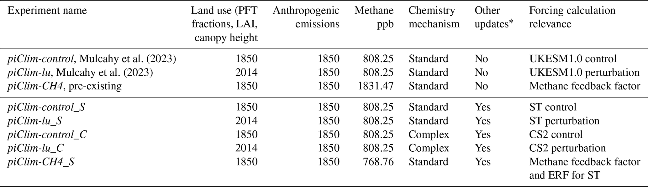
^∗ Other updates: inclusion of organically mediated boundary layer nucleation; updated hygroscopicity values, reaction rates and BVOC emission factors; contribution to SOA from isoprene.

We make use of a pre-existing experiment pair from UKESM1.1 (piClim-control and piClim-lu; Mulcahy et al., 2023) and run two new key experiment pairs, which use two different chemistry mechanisms. Two simulations (piClim-control_S and piClim-lu_S) include the additional processes described in the previous subsection (Sect. 2.1), except for the complex chemistry mechanism. As the complex chemistry mechanism has been found to have a substantial influence on BVOC impacts (Weber et al., 2022), it is included alongside other processes in the second experiment pair (piClim-control_C and piClim-lu_C). Two additional experiments (the pre-existing piClim-CH4 and new piClim-CH4_S) were used to calculate the methane (CH₄) feedback factor on its own lifetime. Further, the piClim-CH4_S experiment can be used to calculate the CH₄ effective radiative forcing (ERF${}_{{\mathrm{CH}}_{\mathrm{4}}}$) associated with land use change.

2.3 Radiative forcing calculations

The net simulated land use effective radiative forcing (ERF_LU) is calculated based on the change in the net incoming (downwelling − upwelling) top of atmosphere (TOA) fluxes in both the shortwave (SW) and longwave (LW) between the land use perturbation experiment (piClim-lu_S or piClim-lu_C) and the respective control (piClim-control_S or piClim-control_C) simulations. The methodology to quantify the forcing associated with a particular gas, aerosol effects or surface albedo varies; the approaches used are described in more detail in the paragraphs below.

The recommendations of Ghan (2013) are followed to calculate the instantaneous radiative forcing (IRF) from aerosol-radiation interactions (IRF_ARI), as well as the cloud forcing from changes in cloud-radiative effects (ΔCRE):

$$\begin{array}{}\text{(1)}& {\displaystyle }{\mathrm{IRF}}_{\mathrm{ARI}}=\mathrm{\Delta }(F-F_{\mathrm{clean}})\text{(2)}& {\displaystyle }\mathrm{\Delta }\mathrm{CRE}=\mathrm{\Delta }(F_{\mathrm{clean}}-F_{\mathrm{clear},\mathrm{clean}})\end{array}$$

where F is the TOA radiative flux (downwelling − upwelling), F_clean is the TOA radiative flux excluding scattering and absorption by aerosols and F_clear,clean is the TOA radiative flux excluding cloud effects and scattering and absorption by aerosols. The calculation of radiative fluxes multiple times with different forcings included is referred to as the double call method. The aerosol-free fluxes are used to calculate the CRE, as aerosols above clouds also interact with the radiation and can bias the forcing diagnosis at TOA (Ghan, 2013).

A double call to the radiation scheme is also used to calculate the instantaneous radiative forcing driven by changes in ozone concentrations (IRF${}_{{\mathrm{O}}_{\mathrm{3}}}$). For each simulation, the radiative fluxes are calculated once using a reference O₃ distribution and once using the simulated O₃ concentrations. The same reference distribution data, in this case monthly mass mixing ratios for the year 2014, are used for all simulations, so that the difference between the reference and simulated O₃ radiative fluxes can be compared between simulations to calculate IRF${}_{{\mathrm{O}}_{\mathrm{3}}}$ (Collins et al., 2025).

The surface albedo forcing (RF_Alb,surf) is calculated following Weber et al. (2024):

$$\begin{array}{}\text{(3)}& {\mathrm{RF}}_{\mathrm{Alb}}=\mathrm{\Delta }{F}_{\mathrm{surf},\mathrm{clear},\mathrm{clean}}\times {\displaystyle \frac{{\mathrm{SW}}_{\mathrm{DW},\mathrm{surf},\mathrm{clean}}}{{\mathrm{SW}}_{\mathrm{DW},\mathrm{surf},\mathrm{clear},\mathrm{clean}}}}\end{array}$$

where $F_{\mathrm{surf},\mathrm{clear},\mathrm{clean}}$ is the surface flux excluding scattering by aerosols and clouds, and (${\mathrm{SW}}_{\mathrm{DW},\mathrm{surf},\mathrm{clean}}/{\mathrm{SW}}_{\mathrm{DW},\mathrm{surf},\mathrm{clear},\mathrm{clean}}$) is the ratio of the downwelling SW clean (excluding scattering and absorption by aerosols) to SW clear-clean (excluding scattering and absorption by aerosols and clouds) fluxes at the surface. This method is used so that the albedo effect is not amplified by the removal of the cloud and aerosol effects, which permits a higher proportion of SW radiation to directly reach the surface/TOA. However, the RF_Alb,surf is quantified at the surface, whereas the aerosol and O₃ forcings are calculated at the TOA. The presence of SW absorbing trace gases and aerosols in the atmosphere means not all of the reflected radiation would reach the TOA.

Two alternative surface albedo forcing calculations, which are valid at the TOA, are also explored to test the sensitivity of this result to the methodology. The simplest method makes the assumption that the change in SW TOA fluxes excluding scattering and absorption by aerosols and clouds is predominantly due to changes in surface albedo (Ghan, 2013), so that

$$\begin{array}{}\text{(4)}& {\mathrm{RF}}_{\mathrm{Alb},\mathrm{clear},\mathrm{clean},\mathrm{TOA}}=\mathrm{\Delta }{F}_{\mathrm{SW},\mathrm{clear},\mathrm{clean}}.\end{array}$$

This method is expected to overestimate the albedo forcing, as the masking effect of clouds and aerosols is completely removed. Finally, the forcing can be estimated from the clear-sky change in surface albedo, the incident SW radiation at the top of atmosphere and the clear-sky atmospheric transmissivity (0.7) following Qu and Hall (2006) and Collins et al. (2025):

$$\begin{array}{}\text{(5)}& {\mathrm{RF}}_{\mathrm{Alb},\mathrm{clear},\mathrm{TOA}}=-\mathrm{0.7}\times \mathrm{\Delta }\mathrm{Albedo}\times {\mathrm{SW}}_{\mathrm{DW},\mathrm{TOA}}.\end{array}$$

This method includes a correction for the effects of gases and aerosols in the atmosphere that interact with the reflected SW radiation and provides an estimate for the TOA surface albedo forcing. However, the masking effect of clouds is not included.

The impacts of changes to CH₄ and CO₂ are not included in the net ERF_LU calculated from the land use perturbation simulation pairs, as the concentrations of both greenhouse gases are prescribed. Two methods are used to calculate the CH₄ forcing for the standard chemistry mechanism, but only method one is applied for the complex chemistry mechanism due to the high computational cost of the second approach. The first method follows a multi-step process to estimate the RF${}_{{\mathrm{CH}}_{\mathrm{4}}}$ based on the change in CH₄ concentration expected from the difference in CH₄ lifetime between the simulation pairs. The CH₄ lifetime for each simulation is initially calculated against removal by OH, but adjusted for stratospheric and soil sinks, following Holmes (2018). Next, the change in CH₄ concentration based on these lifetimes is calculated as in multiple previous studies (e.g. O'Connor et al., 2021; Weber et al., 2024; Stevenson et al., 2013; Fiore et al., 2009):

$$\begin{array}{}\text{(6)}& [\mathrm{CH}\mathrm{4}{]}_{\text{piClim-LU}}=[\mathrm{CH}\mathrm{4}{]}_{\text{piClim-control}}\times {\left({\displaystyle \frac{{\mathit{\tau }}_{\text{piClim-LU}}}{{\mathit{\tau }}_{\text{piClim-control}}}}\right)}^f\end{array}$$

where [CH4] is the CH₄ concentration, τ is the CH₄ lifetime and f is the feedback factor accounting for the feedback of CH₄ on its own lifetime (Prather, 1996). Changes in CH₄ affect OH concentrations, which in turn impact CH₄ oxidation and lifetime (O'Connor et al., 2010; Voulgarakis et al., 2013). We note the CH₄ feedback on its own lifetime varies depending on the Earth system model and background state of the atmosphere. We first calculate f based on outputs from pre-existing UKESM1.1 simulations (piClim-control and piClim-CH4) and the following equations:

$$\begin{array}{}\text{(7)}& f=\mathrm{1}/(\mathrm{1}-s)\end{array}$$

where:

$$\begin{array}{}\text{(8)}& s={\displaystyle \frac{\mathrm{\Delta }\ln \mathit{\tau }}{\mathrm{\Delta }\ln \left[\mathrm{CH}\mathrm{4}\right]}}.\end{array}$$

Next, the direct radiative effect from changes in CH₄ concentrations is calculated following Etminan et al. (2016):

$$\begin{array}{}\text{(9)}& {\mathrm{RF}}_{\mathrm{CH}\mathrm{4}\mathrm{init}}=\left[a\stackrel{\mathrm{‾}}{M}+b\stackrel{\mathrm{‾}}{N}+\mathrm{0.043}\right]\times \left(\sqrt{M}-\sqrt{M_{\mathrm{0}}}\right)\end{array}$$

where a and b are constants ($a=-\mathrm{1.3}\times {\mathrm{10}}^{-\mathrm{6}}$ W m⁻² ppb⁻¹ and $b=-\mathrm{8.2}\times {\mathrm{10}}^{-\mathrm{6}}$ W m⁻² ppb⁻¹), M is the concentration of CH₄ (ppb) that would arise following the land cover change if the modelled concentration was free to evolve, M₀ is the prescribed PI concentration, while $\stackrel{\mathrm{‾}}{M}$ is the mean of the two concentrations of CH₄. $\stackrel{\mathrm{‾}}{N}$ refers to the PI concentration of N₂O (ppb) in this case. Finally, RF_CH4init is scaled to account for methane's indirect radiative effects due to its impacts on O₃ and stratospheric water vapour production, as well as the cloud radiative effect. Previous research based on multi-model assessments suggested a scaling of 1.31 (Smith et al., 2018; Thornhill et al., 2021a; Weber et al., 2024). However, this scaling may not be representative of UKESM. Instead, the decomposition of the CH₄ forcing specifically in UKESM1.0 (O'Connor et al., 2022) is used to estimate the scaling. This UKESM-specific scaling is between 1.43 and 1.96 based on the ratio of the total PI-to-PD ERF${}_{{\mathrm{CH}}_{\mathrm{4}}}$, which includes all indirect effects, to the PI-to-PD ERF from changes in CH₄ concentrations alone. The range represents the uncertainty in the simulation results. The indirect radiative effects of CH₄ are assumed to scale linearly with the magnitude of the change in CH₄ concentration for this calculation.

The second method to calculate the CH₄ forcing is based on the additional experiment piClim-CH4_S introduced in the previous section, for which the CH₄ concentration calculated in method one was prescribed. The difference in TOA fluxes between piClim-CH4_S and piClim-control_S represents the ERF${}_{{\mathrm{CH}}_{\mathrm{4}}}$ when the standard chemistry mechanism is used. We also use the comparison between these two simulations to calculate the CH₄ feedback on its own lifetime in our modelling set up; we find that the difference between UKESM1.1 and the model set up used here with the standard chemistry mechanism is not substantial (1.31 vs. 1.29). We were not, however, able to calculate a separate estimate for the feedback when the complex chemistry is used with the available simulations.

Finally, the CO₂ forcing (RF${}_{{\mathrm{CO}}_{\mathrm{2}}}$) from the land use change is calculated following Etminan et al. (2016):

$$\begin{array}{}\text{(10)}& \begin{array}{rl}{\mathrm{RF}}_{{\mathrm{CO}}_{\mathrm{2}}}=& \left[a_{\mathrm{1}}(C-C_{\mathrm{0}}{)}^{\mathrm{2}}+b_{\mathrm{1}}|C-C_{\mathrm{0}}|+c_{\mathrm{1}}\stackrel{\mathrm{‾}}{N}+\mathrm{5.36}\right]\\ & \times \ln (C/C_{\mathrm{0}})\end{array}\end{array}$$

where a₁, b₁ and c₁ are constants ($a_{\mathrm{1}}=-\mathrm{2.4}\times {\mathrm{10}}^{-\mathrm{7}}$ W m⁻² ppm⁻¹; $b_{\mathrm{1}}=\mathrm{7.2}\times {\mathrm{10}}^{-\mathrm{4}}$ W m⁻² ppm⁻¹, $c_{\mathrm{1}}=-\mathrm{2.1}\times {\mathrm{10}}^{-\mathrm{4}}$ W m⁻² ppb⁻¹), C is the concentration of CO₂ (ppm) that would arise following the land cover change if the modelled concentration was free to evolve, C₀ is the prescribed PI concentration, while $\stackrel{\mathrm{‾}}{N}$ refers to the PI concentration of N₂O (ppb). The change in CO₂ concentration is calculated based on the historical land use carbon emission data provided for the Coupled Climate–Carbon Cycle Model Intercomparison Project (C4MIP) (Jones et al., 2016). An airborne fraction of 0.5 for the carbon emissions (Bennett et al., 2024) is used to calculate the resulting change in atmospheric CO₂.

3 Results

3.1 Land cover change between 1850 and 2014

The PI to PD land use change is dominated by the loss of forest cover, both broadleaf and needleleaf, in favour of grasslands (Fig. 1). Regions of particularly substantial change include central and eastern North America and the southern hemisphere (SH) (sub)tropics, where some areas lose over 50 % of their forest cover. The northern hemisphere (NH) mid-to-high-latitude changes involve both broadleaf and needleleaf forests, while predominantly broadleaf forests are diminished at low latitudes (Fig. 1e). Smaller scale changes occur in southern Africa and central Eurasia. Conversely, in the European Alps, grasses are replaced by shrubs and needleleaf forests. The changes in land cover are reflected in the leaf area index (LAI), which decreases where forests are converted to grasslands (Fig. S1 in the Supplement). Overall, the PI to PD land use change results in a loss of 14 % of the global forest cover (Table 2), which drives a decrease in the global mean LAI by 0.16 (−8 %).

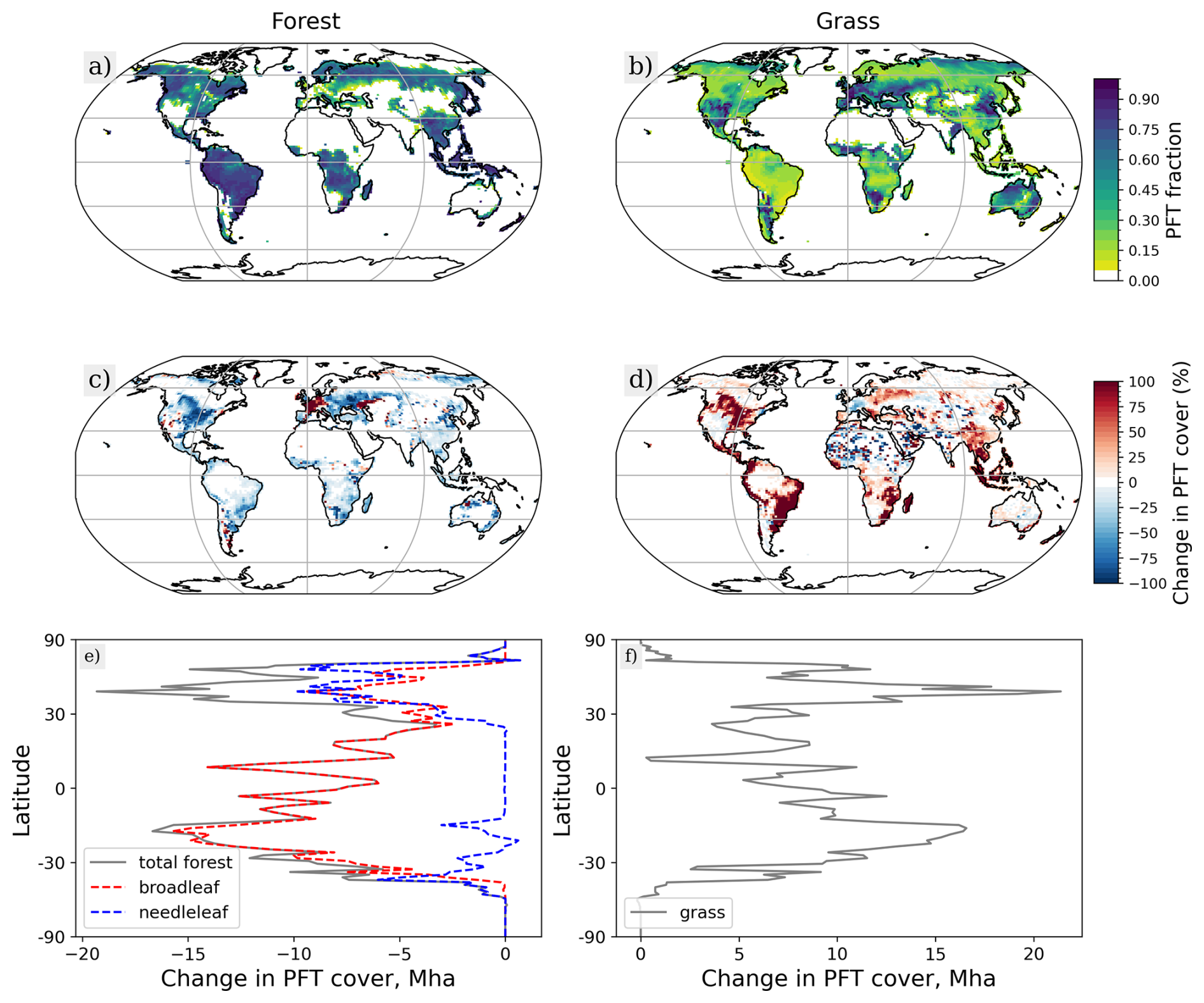
Figure 1 Distribution of the forest (left column) and grass (right column) PFTs. Panels (a) and (b) show the spatial distribution used to represent land cover for 1850. Panels (c) and (d) show the change from pre-industrial to present-day conditions (2014 − 1850) as a % of the 1850 PFT distribution. Panels (e) and (f) show the total change in forest (broadleaf and needleleaf) and grass as a function of latitude.

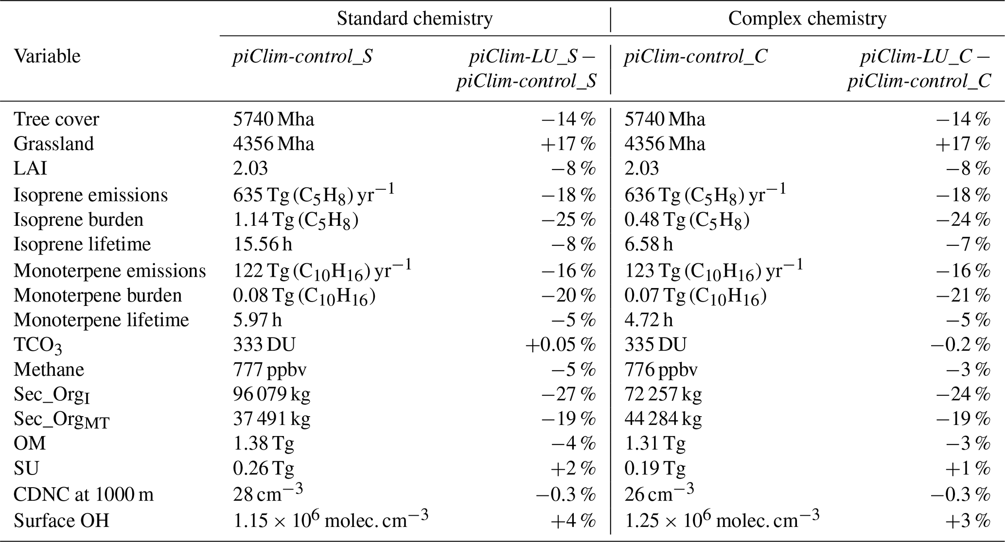
Table 2 Baseline (piClim-control_S or piClim-control_C) values of key variables for both the standard and complex chemistry mechanisms, as well as their relative differences in response to pre-industrial to present-day land use change (e.g. piClim-LU_S − piClim-control_S). The baseline values are given as global sums, except for the BVOC lifetimes, total column ozone (TCO₃), methane concentration, cloud droplet number concentration (CDNC), and surface OH concentration, for which the surface area weighted global mean values are presented.

3.2 Impact of land cover change on BVOC emissions

Consistent with the decrease in high-BVOC-emitting forests in favour of grasslands, the global emissions of isoprene and monoterpenes decrease by around 115 Tg (C₅H₈) yr⁻¹ (−18 %) and 20 Tg (C₁₀H₁₆) yr⁻¹ (−16 %), respectively, as a result of the land cover change (Table 2, Fig. 2), which is comparable to the decrease in BVOC emissions estimated in previous studies of PI to PD land cover impacts (Heald and Spracklen, 2015). The spatial pattern of decreased emissions closely follows that of forest cover loss (or, conversely, grass cover gain). However, the magnitude of the decrease in BVOC emissions is greatest in the tropics. This is due to the higher emission factors of broadleaf forest PFTs, which form a greater proportion of the deforestation at low latitudes, as opposed to needleleaf forest PFTs (compare Figs. 1e and 2e). The decreased emissions lead to decreases in the global burden of isoprene and monoterpenes by 20 % to 25 % (Table 2).

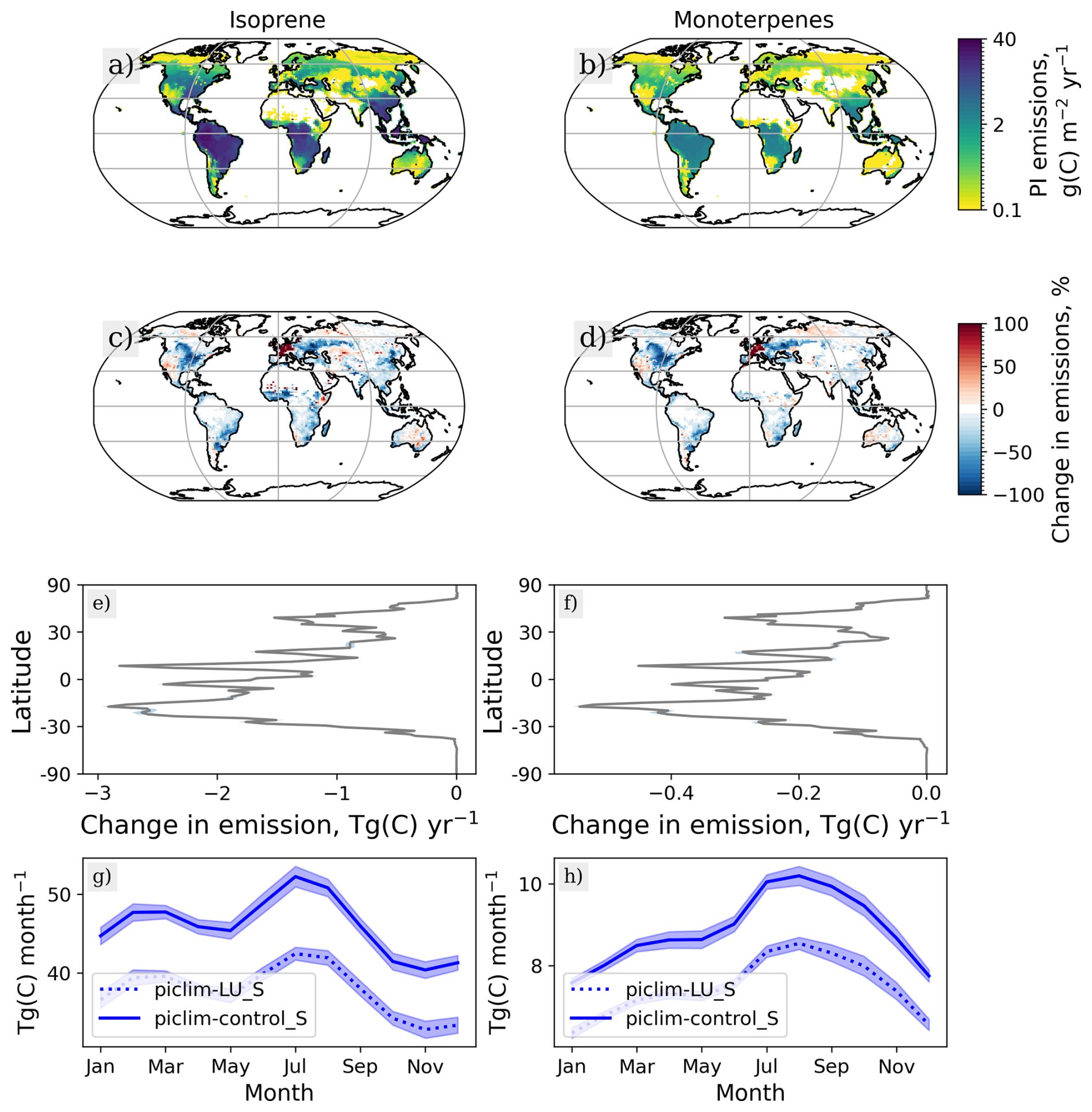
Figure 2 Land cover change impact on BVOC emissions (left column: isoprene, right column: monoterpenes). Panels (a) and (b) show the mean annual emissions of isoprene and monoterpenes for pre-industrial conditions. Panels (c) and (d) show the relative change in the respective emissions when present-day land cover is used. The absolute latitudinal differences are shown on panels (e) and (f), while the the global seasonal cycles from the piClim-control_S and piClim-LU_S experiments are displayed on panels (g) and (h).

The global burdens of both isoprene and monoterpenes are much lower for the simulations with more complex chemistry (Table 2), despite very similar BVOC emission magnitudes. This is driven by the higher oxidising capacity of the atmosphere when the complex mechanism is used (Archer-Nicholls et al., 2021; Weber et al., 2021), driving a 58 % (21 %) decrease in isoprene (monoterpene) lifetime compared to the standard mechanism in the PI simulations. However, the relative change in BVOC burden and lifetime due to land use is largely consistent. For both chemistry mechanisms, the land use-driven decreases in burden are driven by the lower BVOC emissions combined with the 5 % to 8 % shorter lifetimes in the land use perturbation experiments. We attribute these shorter lifetimes to the greater availability of oxidants near source regions when BVOC emissions are decreased following land use changes; the surface level OH concentrations increase by 3 % to 4 % (Table 2).

3.3 Net simulated PI to PD ERF_LU

Figure 3 shows the net simulated effective radiative forcing from PI to PD land use change (ERF_LU) for the standard and complex chemistry experiment pairs. The global mean ERF_LU, which excludes the CO₂ and CH₄ contributions, is $-\mathrm{0.080}\pm \mathrm{0.047}$ W m⁻² with the standard chemistry scheme, while the magnitude of the forcing increases for the complex chemistry scheme to $-\mathrm{0.116}\pm \mathrm{0.041}$ W m⁻². These values include the impacts of changes in aerosols, ozone, cloud properties and surface albedo. The regional nature of land use change results in significant and substantial regional differences in TOA fluxes, despite the relatively small global mean ERF_LU. The dominant latitudinal feature is, on average, the −0.5 or −1.0 W m⁻² forcing at around 50° N for the standard and complex chemistry mechanisms, respectively (Fig. 3b, d), which is consistent with the substantial loss of forest cover at these latitudes. For both mechanisms, the negative forcing is particularly substantial over eastern Europe and central North America, where it regionally reaches −8 W m⁻². Significant impacts are also found on the other continents, for example the average ERF_LU for South America is $-\mathrm{0.57}\pm \mathrm{0.10}$ W m⁻² for the standard chemistry mechanism and $-\mathrm{0.52}\pm \mathrm{11}$ W m⁻² for the complex chemistry (Table S2). The greater magnitude of the NH forcing when employing more complex chemistry is driven by changes in northeast Asia (Fig. 3c); a negative forcing in this region is not present with the standard chemistry scheme.

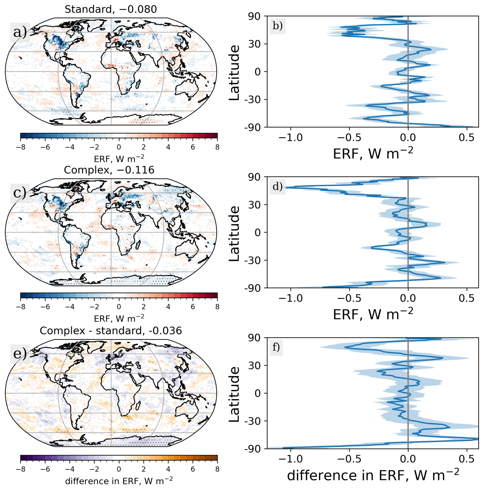
Figure 3 Net simulated TOA land use ERF (ERF_LU) in W m⁻² for the standard chemistry mechanism (a), as well as respective zonal mean values (b). Panels (c) and (d) are the equivalent data for the complex chemistry mechanism. Values over panels (a) and (c) are the global mean ERFs. Panel (e) shows the geographical distribution of the difference in ERF_LU when the chemistry mechanism is changed and panel (f) shows the zonal change in ERF_LU. Stippling on panels (a), (c) and (e) shows differences that are significant based on Student's t-test with 95 % confidence, while shading on the zonal plots shows the standard error.

The other substantial difference between the simulations with different chemical mechanisms occurs in the southern high latitudes, where the latitudinal mean ERF_LU rises to +0.4 W m⁻² when using the standard scheme but is strongly negative (below −0.5 W m⁻²) for the complex chemistry scheme. This latitudinal signal is driven predominantly by regional differences in East Antarctica, which we connect to changes in O₃ (discussed in more detail in Sect. 3.6). The results tend to be more consistent at the lower latitudes, especially in the SH, where the ERF_LU values lie between −0.25 and 0.25 W m⁻², despite the substantial deforestation in the (sub)tropical SH.

3.4 Aerosol-radiation interactions

Figure 4a–c shows the mean instantaneous radiative forcing associated with the aerosol direct effect (IRF_ARI) from land use change. The global average IRF_ARI is $+\mathrm{0.057}\pm \mathrm{0.015}$ and $+\mathrm{0.058}\pm \mathrm{0.011}$ W m⁻² for the standard and complex chemistry mechanisms, respectively. In both cases, the shortwave forcing dominates (+0.058 and +0.056 W m⁻² for the standard and complex mechanisms, respectively; Table 3). IRF_ARI values tend to increase closer to the equator, although there is a secondary peak in the forcing in the NH mid-to-high-latitudes (Fig. 4c). On a continental scale, the greatest magnitude average forcing occurs in sub-Sahel Africa (over +0.20 W m⁻²; Table S2).

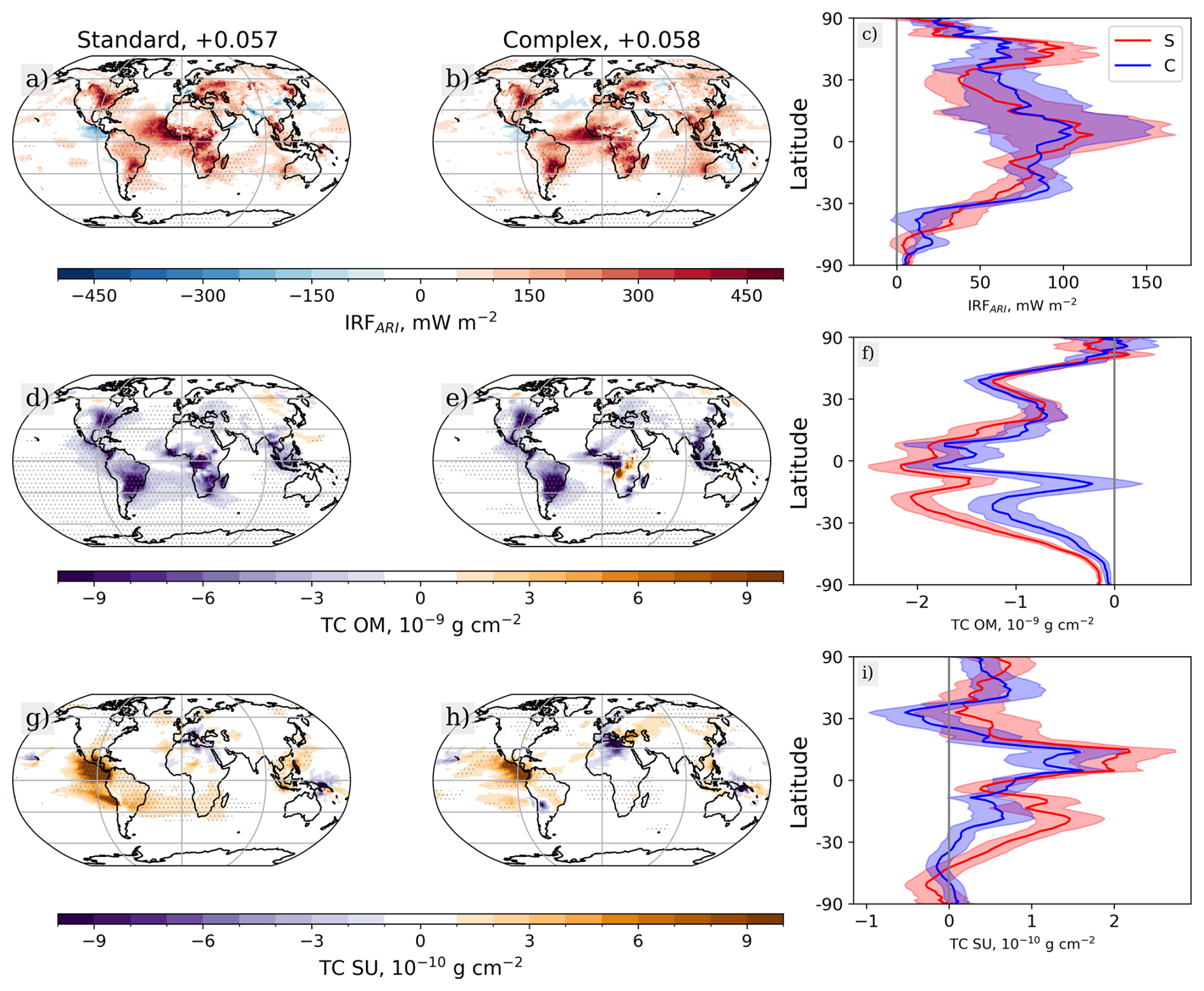
Figure 4 The role of aerosol-radiation interactions in pre-industrial to present-day land use forcing. Panels (a)–(c) show the top of atmosphere IRF from ARI associated with land cover changes for the standard (s, left column) and complex (c, middle column) chemistry mechanism, as well as the zonal mean values of IRF_ARI values for both mechanisms (right column). The changes in total column organic matter (OM) mass are displayed in panels (d), (e) and (f), while panels (g), (h) and (i) show the differences in total column sulphate (SU) mass. Stippling in the left and middle columns shows regions of significant differences based on Student's t-test with 95 % confidence, while shading on the zonal plots shows the standard error.

Table 3 Decomposition of the pre-industrial to present-day land use radiative forcing in mW m⁻².

The positive IRF_ARI values are driven by a decrease in aerosol burden, which results in less scattering and reflection of SW radiation. Global organic matter (OM) burdens decrease by 3 % to 4 % (Table 2). Figure 4d–f shows how the decreases in total column OM occur in the same regions as the positive IRF_ARI. The decreases are also greatest near the equator, where the BVOC emissions decrease by the greatest amounts (Sect. 3.2), and where the highest magnitude of IRF_ARI is found. The magnitude of the decrease in OM mass is slightly greater for the standard chemistry mechanism than for the more complex mechanism, particularly in the SH. As the atmospheric oxidation capacity is lower when the standard mechanism is used, trace gases have longer lifetimes and can be transported further from source, resulting in the changes secondary aerosol occurring over a greater area (compare Fig. 4d and e).

While the global mean IRF_ARI values are positive, we note there are some regions of significant negative forcing, particularly in Central America. These regional impacts can be connected to an increase in sulphate aerosol in these regions (Fig. 4g–i). The decrease in BVOC emissions and burden under land use change increases the availability of the hydroxyl radical (OH), one of the main oxidants of sulphur dioxide (SO₂). As a result, aerosol formation and growth reactions occur closer to source regions, leading to greater sulphate aerosol burdens in these areas. Additionally, a slight shift occurs in the sulphate formation and growth pathways; there is an < 2 percentage point increase in the relative contribution from reactions with OH (Table S1). The OH nucleation and condensation fluxes increase, regionally by over 50 %, where BVOC emission fluxes have decreased and the availability of OH in the lower troposphere has increased (compare Figs. 2, S2 and S3). These changes potentially lead to a shift to more numerous but smaller sulphate particles (Karset et al., 2018; O'Connor et al., 2022). The impacts on sulphate aerosol are greater for the standard mechanism, where the oxidation capacity is more sensitive to changes in BVOC emissions (Sands et al., 2025).

3.5 Cloud radiative effect

The magnitude of the change in the global mean cloud radiative effect (ΔCRE) associated with pre-industrial (PI) to present-day (PD) land use change is very similar for both the standard chemistry mechanism ($+\mathrm{0.087}\pm \mathrm{0.033}$ W m⁻²) and the complex mechanism ($+\mathrm{0.082}\pm \mathrm{0.025}$ W m⁻²). However, the effect is almost limited to changes in the SW for the standard mechanism (ΔCRE${}_{\mathrm{SW}}=+\mathrm{0.086}\pm \mathrm{0.030}$ W m⁻², Fig. 5a), whereas LW fluxes are more affected for the complex mechanism (ΔCRE${}_{\mathrm{SW}}=+\mathrm{0.047}\pm \mathrm{0.027}$ W m⁻², ΔCRE${}_{\mathrm{LW}}=+\mathrm{0.035}\pm \mathrm{0.019}$ W m⁻²; Table 3), although the decomposed ΔCRE still overlap due to the substantial standard error.

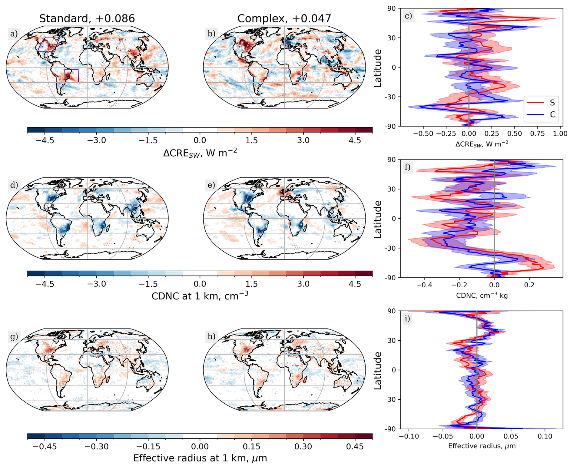
Figure 5 The role of the cloud radiative effect (CRE) in pre-industrial to present-day land use forcing. Panels (a)–(c) show changes in the top of atmosphere fluxes from ΔCRE_SW associated with land cover changes for the standard (s, left column) and complex (c, middle column) chemistry mechanism, as well as the zonal mean ΔCRE_SW values for both mechanisms (right column). The changes in cloud droplet number concentrations (CDNC) at 1 km altitude are displayed in panels (d), (e) and (f), while panels (g), (h) and (i) show the differences in effective radius at 1 km altitude. Stippling in the left and middle columns shows regions of significant differences based on Student's t-test with 95 % confidence, while shading on the zonal plots shows the standard error. The purple boxes on panel (a) mark regions of more substantial ΔCRE_SW impacts that have been studied in additional detail.

The ΔCRE tends to be positive over regions of substantial deforestation, such as central North America (regional average $+\mathrm{0.50}\pm \mathrm{0.17}$ and $+\mathrm{0.91}\pm \mathrm{0.18}$ W m⁻² for the standard and complex mechanisms, respectively) and eastern South America ($+\mathrm{0.72}\pm \mathrm{0.13}$ and $+\mathrm{0.60}\pm \mathrm{0.12}$ W m⁻²). The positive ΔCRE_SW is likely due to the changes in aerosols, introduced in the previous section (Sect. 3.4), driving a decrease in the cloud droplet number concentration (CDNC) as the aerosol burden is reduced. The CDNC at 1 km altitude tends to decrease over regions of deforestation (Fig. 5d–f), in turn leading to an increase in the effective radius of the cloud droplets (Fig. 5g–i). These changes decrease the amount of incoming radiation reflected by the cloud, resulting in a positive forcing (i.e. the so-called Twomey effect is weaker; Twomey, 1977).

Table 4 The impact of PI to PD land use change on regional OM burden, CCN, CDNC at 1 km altitude and ΔCRE_SW. The two regions studied (central North America and eastern South America) are highlighted on Fig. 5a.

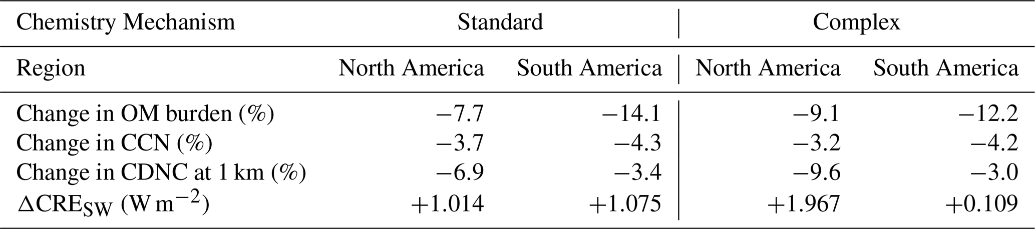
The connection between lower organic aerosol loading and fewer cloud droplets is particularly apparent in central North America and eastern South America and is analysed in more detail here (see regions highlighted on Fig. 5a). The decrease in OM burden globally in response to land use change is greater in magnitude than the change in sulfate burden (Fig. 4 and Table 2). Table 4 shows that OM burdens decrease by 7.7 % to 14.1 % in the identified regions. This is associated with a decrease in cloud condensation nuclei (CCN; aerosol particles > 70 nm in diameter) by 3 % to 4 %, which in turn drives a decrease in CDNC (from −3.0 % in South America to −9.6 % in North America; Figs. S4–S6). This decrease in CDNC is the likely mechanism behind the positive regional ΔCRE_SW, which is greater than 1 W m⁻², except for the South America region when using the complex chemistry mechanism. The lower magnitude of the radiative impacts in South America suggests other mechanisms may also be relevant in that region.

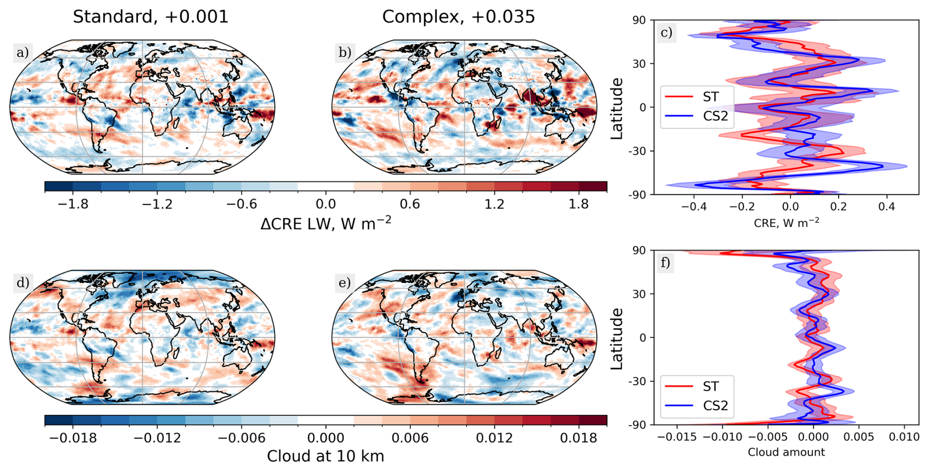
Figure 6 The change in longwave cloud radiative effect between present-day and pre-industrial conditions for the standard (a) and complex (b) chemistry mechanism, as well as the zonal mean values for both (right column). The change in cloud amount (as a fraction of the grid cell) at 10 km altitude for the standard (d) and complex (e) chemistry mechanisms, and the zonal mean cloud amount for both (f).

The method for calculating the ΔCRE used in this study will also capture differences due to changes in cloud amount and/or the location and lifetime of clouds, all of which may also be influenced by changes in water vapour or atmospheric dynamics. While the impacts of these changes are not investigated separately in detail here, and they may contribute to noted difference in ΔCRE_SW, the spatial pattern of ΔCRE_LW closely resembles the changes in average cloud amount at 10 km altitude (Fig. 6). This high-altitude cloud amount increases over a 3 % larger area when the complex chemistry mechanism is used. The greater change in ΔCRE_LW with the complex mechanism could be driven by these differences in high-level clouds. An increase in cirrus-type clouds reduces the amount of outgoing LW radiation and leads to a positive forcing (Chen et al., 2000). However, the uncertainty in the results, particularly for ΔCRE_LW, is substantial and more in-depth analysis of the upper-tropospheric cloud formation is required for a robust understanding of the forcing mechanism.

3.6 O₃ contribution to ERF_LU

The mean O₃ instantaneous radiative forcing (IRF${}_{{\mathrm{O}}_{\mathrm{3}}}$) associated with the pre-industrial (PI) to present-day (PD) land use change is shown in Fig. 7a and b. While the global mean values are weakly negative ($-\mathrm{0.003}\pm \mathrm{0.012}$ and $-\mathrm{0.015}\pm \mathrm{0.009}$ W m⁻² for the standard and complex chemistry mechanisms, respectively), the standard errors are substantial and there are regions of positive forcing, particularly in regions associated with the NH polar jet stream. The major difference between the two chemistry mechanisms is the sign of IRF${}_{{\mathrm{O}}_{\mathrm{3}}}$ over East Antarctica, which seems to be driving the difference in ERF_LU between the two mechanisms in this region. For the standard chemistry mechanism, the IRF${}_{{\mathrm{O}}_{\mathrm{3}}}$ is positive (< +0.1 W m⁻²) here, whereas the complex chemistry results in a negative forcing of a similar magnitude.

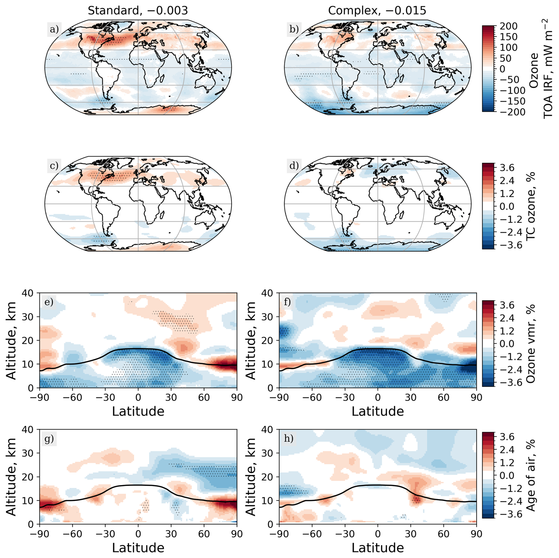
Figure 7 Contribution to pre-industrial to present-day land use forcing from changes in ozone. Changes in the TOA IRF from changes in O₃ concentrations in mW m⁻² for the standard (a, left column) and complex (b, right column) chemistry mechanisms are compared to changes in TC O₃ (c, d). Values above panels (a) and (b) show the global mean IRF${}_{{\mathrm{O}}_{\mathrm{3}}}$ in W m⁻². Changes in tropospheric and stratospheric O₃ volume mixing ratios are shown on panels (e) and (f), while the change in the age of air is displayed on panels (g) and (h). Stippling indicates significant differences based on Student's t-test with 95 % confidence, while the black line on panels (e)–(h) shows the mean height of the tropopause calculated within the model.

The changes in total column O₃ are mostly insignificant, though some significant differences closely resemble the patterns in IRF${}_{{\mathrm{O}}_{\mathrm{3}}}$ at latitudes over 30° (Fig. 7c, d). Looking at the O₃ vertical distribution allows for more insight into changes in O₃ and subsequent IRF${}_{{\mathrm{O}}_{\mathrm{3}}}$ impacts. While the O₃ volume mixing ratio tends to decrease in the troposphere, some increases in O₃ mixing ratios occur at the tropopause and in parts of the stratosphere (Fig. 7e, f). The tropospheric O₃ decrease may be driven by the loss of BVOCs, which are O₃ precursors. Monoterpenes only act as an O₃ precursor in the complex chemistry mechanism, but not in standard scheme (Weber et al., 2021), which would drive a greater magnitude impact on tropospheric O₃ for the complex scheme; the O₃ production fluxes decrease by 1.9 % and 2.9 % in response to land use change for the standard and complex scheme, respectively. However, the small magnitude of the changes in O₃ volume mixing ratios and their high sensitivity to the local chemical environment preclude the identification of a definite cause for the tropospheric variations. We suggest the higher altitude changes in O₃ mixing ratios are driven by dynamical processes. To assess the dynamical influence, the changes in the age of air are shown in Fig. 7g, h. These highlight that the same locations around the tropopause that are associated with substantial differences in O₃ mixing ratios are affected by changes in transport timescales between the troposphere and stratosphere.

3.7 Impact of change to CH₄ lifetime

The experimental set-up includes prescribed methane (CH₄) concentrations, therefore limiting the impact land use change can have on the contribution to ERF_LU from CH₄ forcing. However, as changes in the abundance of BVOCs can affect CH₄ lifetime through changing the availability of OH, we can estimate the change in CH₄ concentration due to land use change (Holmes, 2018). We find the CH₄ lifetime against loss by OH decreases by 4 % and 3 % for the standard and complex mechanisms (Table 5) as a result of land use change, leading to lower equilibrium CH₄ concentrations by 37 and 23 ppbv, respectively. The impact is greater for the standard chemistry scheme, which is consistent with the greater sensitivity of atmospheric oxidants to BVOC emissions for this mechanism.

Table 5 CH₄ lifetimes against OH in the simulations alongside the global mean CH₄ concentrations and top of atmosphere effective radiative forcings from the calculated change in concentration or comparison against piClim-control_S for the CH₄ simulation. Note the CH₄ mixing ratios are calculated from model outputs and vary slightly from the prescribed values.

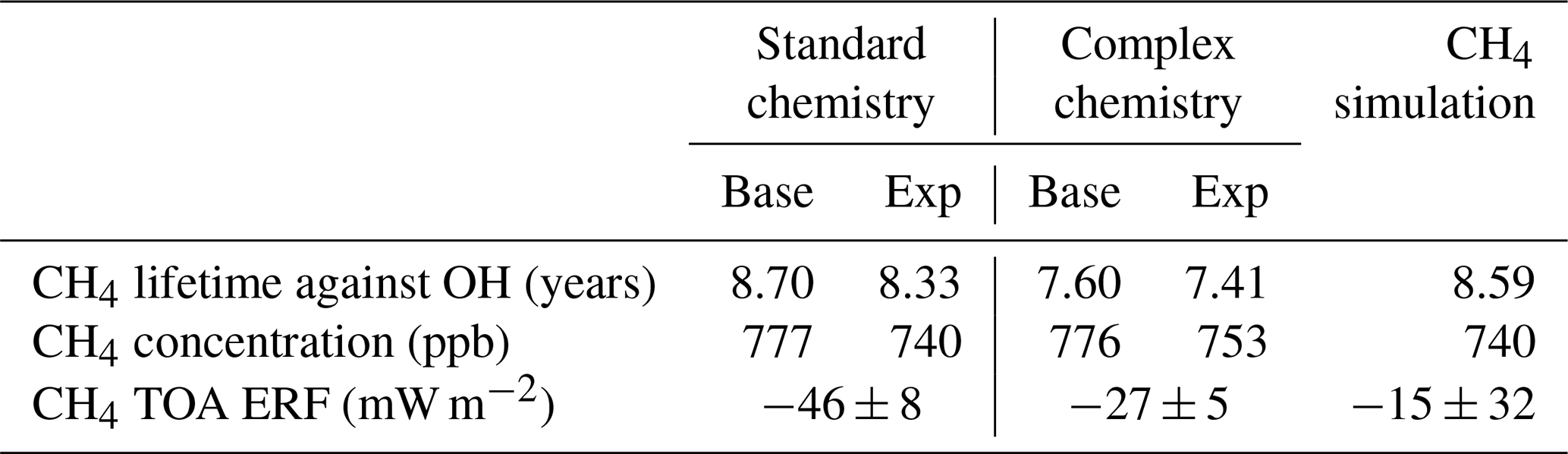
Following the calculated decrease in CH₄ concentrations from PI to PD land use change, the CH₄ effective radiative forcing (ERF${}_{{\mathrm{CH}}_{\mathrm{4}}}$) is negative. The comparison of the additional simulation piClim-CH4_S (see Sect. 2.2 and 2.3), which is set up with a prescribed global mean CH₄ concentration of 740 ppbv consistent with the calculated CH₄ decrease of 37 ppbv, and piClim-control_S suggests the global mean ERF${}_{{\mathrm{CH}}_{\mathrm{4}}}$ is $-\mathrm{0.015}\pm \mathrm{0.043}$ W m⁻² (Table 3). This forcing estimate overlaps with the ERF${}_{{\mathrm{CH}}_{\mathrm{4}}}$ values calculated using the Etminan et al. (2016) equations and additional scalings (see Sect. 2.3) when considering the substantial uncertainty. Based on these calculations, the impact is of a greater magnitude for the standard chemistry ($-\mathrm{0.046}\pm \mathrm{0.008}$ W m⁻²) than the complex chemistry ($-\mathrm{0.027}\pm \mathrm{0.005}$ W m⁻²; Table 5), following the different magnitudes of the changes in concentrations.

3.8 Impacts of biogeophysical effects and changes in CO₂ concentrations

While the focus of this research is on the non-CO₂ biogeochemical impacts of land use change, we recognise that CO₂ emissions, surface albedo and other biogeophysical effects, such evapotranspiration and surface roughness, will also have radiative effects. Here, we quantify the impacts of CO₂ and surface albedo for comparison with non-CO₂ atmospheric composition forcings.

The changes in surface albedo are factored into the net simulated ERF_LU, alongside other geophysical impacts of land cover change, such as differences in evapotranspiration driving changes in water vapour. The global mean surface albedo forcing (RF_Alb,surf; Fig. 8a) calculated following Weber et al. (2024) is similar when using the standard and complex chemistry mechanisms at $-\mathrm{0.174}\pm \mathrm{0.016}$ and $-\mathrm{0.169}\pm \mathrm{0.012}$ W m⁻², respectively (Table 3). The slight difference in RF_Alb,surf, despite the consistent land cover change, is likely driven by the interactive nature of the chemistry and climate in the model; the calculation of RF_Alb,surf depends partially on cloud cover, which will vary between the experiments. Both of these estimates are within the Intergovernmental Panel on Climate Change (IPCC) land use albedo ERF estimate of $-\mathrm{0.2}\pm \mathrm{0.1}$ W m⁻² (IPCC, 2023). Note that RF_Alb,surf is not calculated at the TOA and therefore may not be directly comparable to other forcings that are calculated at the TOA. The alternative TOA calculations of the albedo forcing ($-\mathrm{0.247}\pm \mathrm{0.017}$ and $-\mathrm{0.243}\pm \mathrm{0.019}$ W m⁻²) remain within the IPCC land use albedo ERF estimate. The global mean surface albedo forcing values are, however, greater for both of the alternative methods as they do not account for the masking effect of clouds, which likely leads to an overestimation of the forcing (Fig. 8).

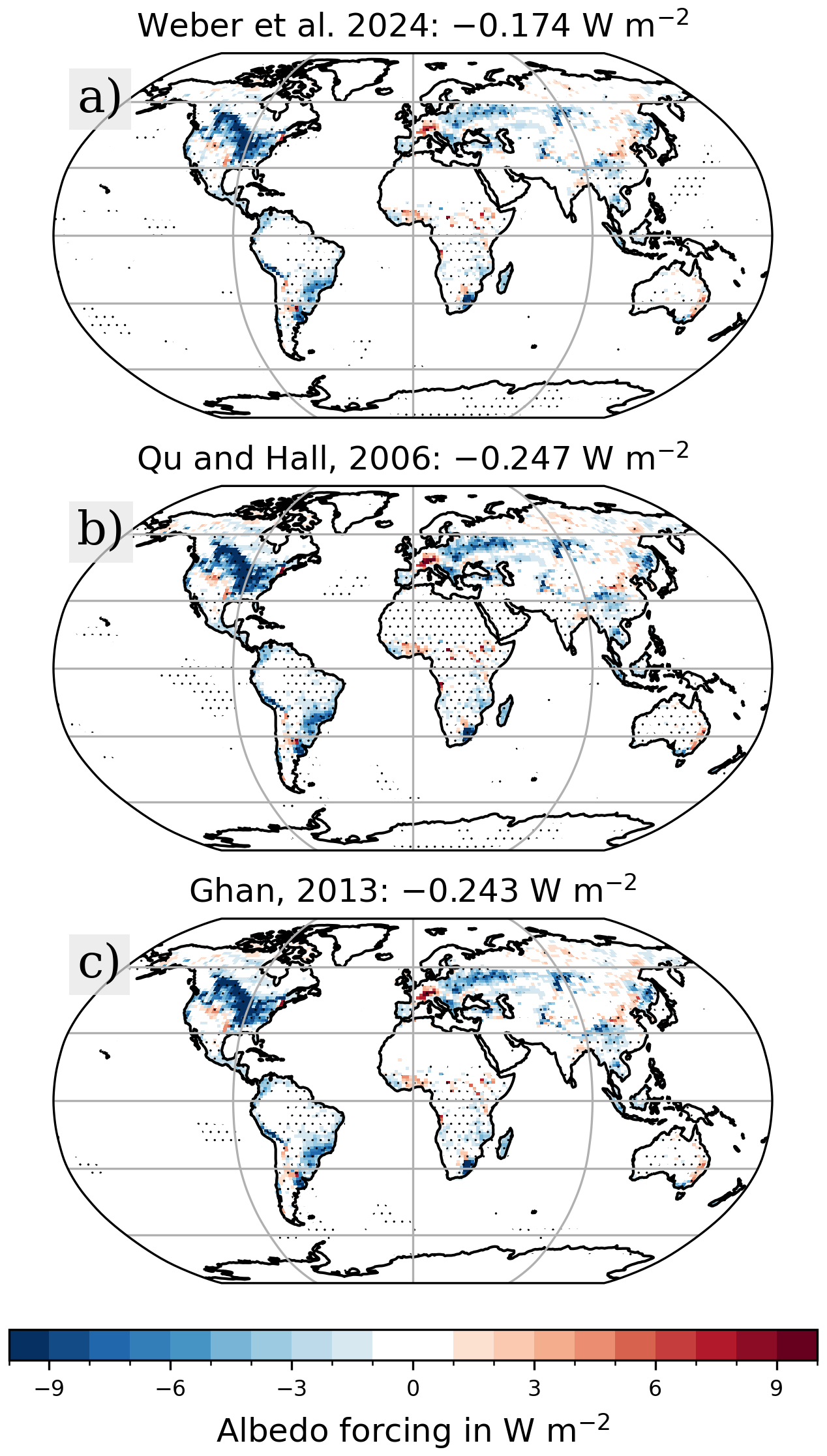
Figure 8 Comparison of 3 methods for albedo forcing calculation based on the experiments employing the standard chemistry mechanism. Panel (a) shows the surface albedo forcing following Weber et al. (2024), which is valid at the Earth's surface, panel (b) shows the change in clear-sky surface fluxes scaled by the clear-sky atmospheric transmissivity (estimated to be 0.7) to get a planetary albedo impact at the TOA (Qu and Hall, 2006; Collins et al., 2025), while panel (c) shows the change in the clear and clean TOA fluxes, thought to be largely due to changes in surface albedo (Ghan, 2013). The stippling shows areas of significant change.

The CO₂ forcing, similarly to that of CH₄, is not included in ERF_LU, due to the prescribed CO₂ concentrations in the experimental set-up. Based on an airborne fraction of 0.5 and the C4MIP land use change carbon emissions (Sect. 2.3), we calculate that atmospheric CO₂ would have increased by 392 Tg CO₂ following the emission of around 214 TgC from land use change between 1850 and 2014. This is equivalent to an increase in atmospheric CO₂ by around 50 ppm. Using the equation from Etminan et al. (2016), this change in CO₂ results in a radiative forcing (RF${}_{{\mathrm{CO}}_{\mathrm{2}}}$) of $+\mathrm{0.867}\pm \mathrm{0.087}$ W m⁻².

3.9 Overview of decomposed LU forcing

In this section, we consider the relative impacts from each of the contributions to the land use change forcing. The largest magnitude forcings associated with changes in atmospheric composition, not including CO₂, are driven by IRF_ARI and ΔCRE (Fig. 9). These, particularly in combination, are much greater than IRF${}_{{\mathrm{O}}_{\mathrm{3}}}$ or ERF${}_{{\mathrm{CH}}_{\mathrm{4}}}$. However, the global mean ERF_LU, despite not including the negative ERF${}_{{\mathrm{CH}}_{\mathrm{4}}}$, is negative, which is connected to the biogeophysical effects. RF_Alb,surf is of a much greater magnitude than the non-CO₂ biogeochemical forcings. Therefore, RF_Alb,surf drives the negative sign of ERF_LU, while the changes in atmospheric trace gases and aerosols modify the magnitude of the net forcing.

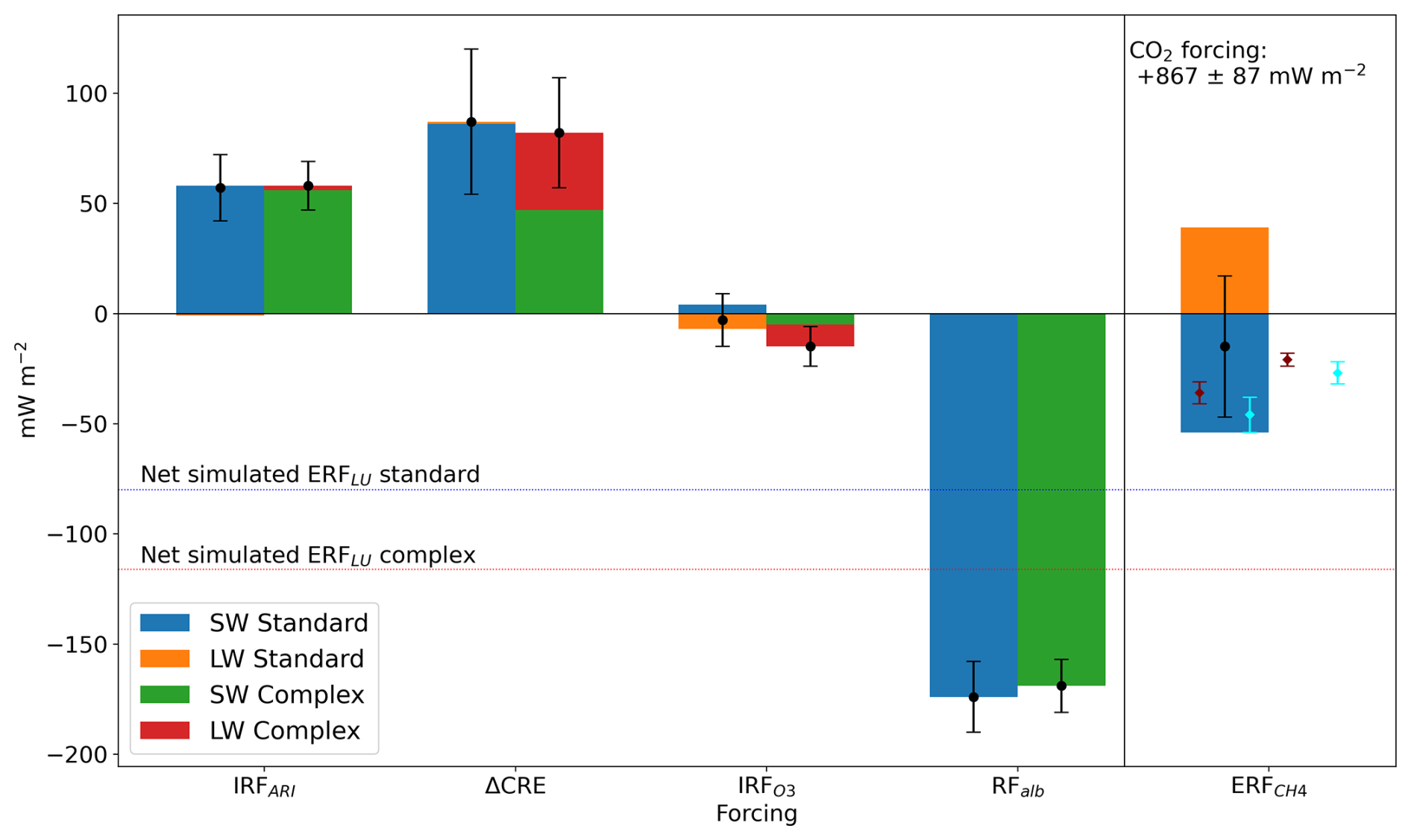
Figure 9 Comparison of forcings for the standard and complex chemistry mechanisms. Note the CH₄ and CO₂ forcing are not included in the net simulated TOA land use ERF, as both of these greenhouse gases are prescribed in the main simulation pairs. The cyan diamonds show the methane forcing calculated using scaling specific to the UKESM, while the maroon diamonds are based on the multi-model scaling.

The non-CO₂ forcings in combination, that is ERF_LU + ERF${}_{{\mathrm{CH}}_{\mathrm{4}}}$, offset only around 15 % of the positive CO₂ forcing from PI to PD land use change emissions. Assuming ERF_LU, ERF${}_{{\mathrm{CH}}_{\mathrm{4}}}$ and RF${}_{{\mathrm{CO}}_{\mathrm{2}}}$ combine linearly, the total PI to PD land use change forcing based on our results is around +0.74 W m⁻², or 34 % [25 % to 48 %] of the change in the net anthropogenic ERF from 1850–1900 to 2006–2019 (IPCC, 2019).

3.10 Comparison to other versions of UKESM (1.0 and standard 1.1)

Table 6 compares the land-use driven changes in TOA fluxes, excluding CH₄ and CO₂ impacts, for four model versions: the experimental set-up used here with both the standard and complex chemistry mechanisms, as well UKESM1.0 and UKESM1.1. This allows for an assessment of the impacts of process and parameter updates (Sect. 2.1; Sands et al., 2025). The net ERF_LU is reduced for both chemistry mechanisms in the new model set-up. The new biosphere-atmosphere processes included in this research reduce ERF_LU from $-\mathrm{0.21}\pm \mathrm{0.04}$ W m⁻² for UKESM1.1 to $-\mathrm{0.08}\pm \mathrm{0.05}$ W m⁻². The impact of new process representation is smaller with the use of the complex chemistry mechanism, for which ERF_LU is $-\mathrm{0.12}\pm \mathrm{0.04}$ W m⁻². While the flux diagnostics for the Ghan (2013) method of decomposing the forcing were not available for UKESM1.1, a more detailed comparison can be made against UKESM1.0, for which ERF_LU is also higher, with a magnitude of $-\mathrm{0.17}\pm \mathrm{0.04}$ W m⁻².

Table 6 Summary of the land use radiative forcing based on top-of-atmosphere fluxes for the standard versions of UKESM1.0 and UKESM1.1, as well as the new simulations presented in this research. NET${}_{\mathrm{CS}}^{\prime }$ is clear-sky forcing that combines changes in trace gases, for example O₃, and in IRF_ARI.

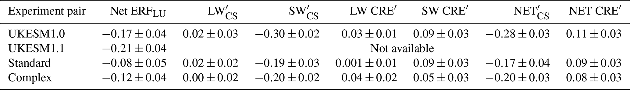
We find the greatest change between model versions occurs for the clear-sky shortwave fluxes (${\mathrm{SW}}_{\mathrm{CS}}^{\prime }={\mathrm{IRF}}_{\mathrm{ARI},\mathrm{SW}}+\mathrm{\Delta }{F}_{\mathrm{clear},\mathrm{clean},\mathrm{SW}}$), which are expected to predominantly be driven by impacts from surface albedo changes and the aerosol-radiation interactions, alongside smaller effects from changes in greenhouse gases. Of all the separated fluxes, the SW${}_{\mathrm{CS}}^{\prime }$ term has the greatest magnitude, regardless of model version. This is also the term that has changed most significantly between UKESM1.0 and the new simulations. SW${}_{\mathrm{CS}}^{\prime }$ is of a much smaller magnitude in the updated model version ($-\mathrm{0.19}\pm \mathrm{0.03}$ and $-\mathrm{0.20}\pm \mathrm{0.02}$ W m⁻² for the standard and complex mechanisms) compared to UKESM1.0 ($-\mathrm{0.30}\pm \mathrm{0.02}$ W m⁻²). Both surface albedo, due to tuning the snow burial of vegetation, and sulphate aerosol representations have been adjusted between UKESM1.0 and UKESM1.1, which may drive some of the differences in SW${}_{\mathrm{CS}}^{\prime }$ (Mulcahy et al., 2023). The new process representation included in the model simulations further changes the spatial distribution of BVOC emissions and the formation and growth of aerosols. The difference in the net ERF_LU between the new standard and complex experiment pairs is 0.04 W m⁻². This is less or equal to the uncertainty associated with each ERF_LU, which highlights that the combination of other process updates from UKESM1.1 has had a greater impact on the net ERF_LU than the choice of chemistry mechanism.

4 Discussion and conclusions

The contributions of O₃, ARI and the CRE to the pre-industrial to present-day land use change radiative forcing have been investigated in an updated configuration of the UK's Earth System Model from UKESM1.1. The net simulated ERF_LU ($-\mathrm{0.08}\pm \mathrm{0.05}$ or $-\mathrm{0.12}\pm \mathrm{0.04}$ W m⁻² depending on the chemistry mechanism) is dominated by a negative forcing from changes in surface albedo. However, the positive IRF_ARI ($+\mathrm{0.06}\pm \mathrm{0.02}$ or $+\mathrm{0.06}\pm \mathrm{0.01}$ W m⁻²) and ΔCRE ($+\mathrm{0.09}\pm \mathrm{0.03}$ or $+\mathrm{0.08}\pm \mathrm{0.03}$ W m⁻²) offset a substantial part of this forcing. Separate calculations reveal changes in CH₄ lifetime as another negative forcing contribution, while increased CO₂ concentrations from land use carbon emissions have a positive forcing, leading to a total forcing (ERF_LU + ERF${}_{{\mathrm{CH}}_{\mathrm{4}}}$ + RF${}_{{\mathrm{CO}}_{\mathrm{2}}}$) of +0.74 W m⁻². The net ERF_LU is similar to the estimates of Unger (2014a, b) ($-\mathrm{0.11}\pm \mathrm{0.17}$ and −0.17 W m⁻²), while the total land use forcing inclusive of changes in CH₄ and CO₂ is within the uncertainty of the estimate of $+\mathrm{0.9}\pm \mathrm{0.5}$ W m⁻² calculated by Ward et al. (2014), who also include CO₂ impacts. These results are also mostly consistent with existing land use radiative forcing studies in terms of the sign of the land use change forcing associated with particular pathways.

Changes in O₃ mixing ratios and CH₄ lifetime have a negative forcing, while aerosol effects, both direct and indirect, tend to have a positive forcing, as previously found by Unger (2014a, b), Heald and Geddes (2016), and Scott et al. (2017). The O₃ forcing magnitude is in line with more recent experiments (e.g. Heald and Geddes, 2016; Scott et al., 2017), which suggest O₃ forcings of less than 0.03 W m⁻². To the best of our knowledge, this study is the first to find a potential change in stratospheric ozone from PI to PD land use change. The calculated CH₄ forcing is between that estimated by Scott et al. (2017) and Unger (2014a, b).

There are more differences compared with existing studies in the magnitude of the aerosol effects. Heald and Geddes (2016) show a negative forcing associated with an increase in nitrate aerosol, while all the aerosol forcings calculated here are positive. Nitrate aerosol is not included in the experimental setup used here, so the overall aerosol burden decreases and any increases due to agricultural emissions are not captured. We expect the inclusion of agricultural emissions in future experiments would result in a substantial increase in nitrate aerosol loading, which would have an opposite forcing through aerosol-radiation interactions to the simulated decrease in organic matter, and could result in a net aerosol forcing more similar to that calculated by Heald and Geddes (2016). Further, the indirect effects of aerosol calculated here are of a greater magnitude than those calculated by Scott et al. (2017). This may be due to Scott et al. (2017) using present-day conditions as the control, in which changes in biogenic aerosol have a much smaller impact relative to the total amount of aerosol compared with simulations using pre-industrial conditions. The sensitivity of aerosol effects to background conditions has been previously highlighted by Carslaw et al. (2017, 2013). In fact, an earlier study by Scott et al. (2014) highlights the sensitivity of the ΔCRE to background aerosol concentrations when testing the impacts of including organically mediated nucleation on BVOC radiative impacts. The cloud adjustments from PI to PD land use change as simulated by CMIP6 models were compared by Smith et al. (2020). The magnitude of the cloud effects ranged from −0.09 to 0.24 W m⁻². The highest positive value was associated with NorESM2-LM, a model that also included interactive BVOC emissions. This enabled the land use change to impact on organic aerosol and, subsequently, CDNC, leading to more positive ΔCRE. The results calculated here are within the range of CMIP6 models, although the cloud forcing is greater than found for the CMIP6 implementation of UKESM1-0-LL.

From a process understanding perspective, the results can also be compared to other land cover or BVOC emission change experiments, even if they do not focus on pre-industrial to present-day transitions. The standard and complex chemistry mechanisms have recently been compared in experiments that quantified the effects of a two factor increase in BVOC emissions in UKESM1.0 under pre-industrial conditions (Weber et al., 2022). As found here, CH₄ responded more strongly to changes in BVOC emissions in the standard chemistry mechanism. The resulting radiative forcings tended to be of the opposite sign to the PI-to-PD land use forcing, consistent with the opposite directions of change in BVOC emissions. However, Weber et al. (2022) found a positive ΔCRE when increasing BVOC emissions, while our results show a positive ΔCRE in response to reduced BVOC emissions. The difference could be driven by the different spatial patterns of BVOC emission changes or the increased hygroscopicity of organic aerosols and reduced hygroscopicity of sulphate aerosols in the new simulations. Weber et al. (2022) attribute the positive ΔCRE to changes in sulphate aerosol driven by a reduction in OH. The change in process representation, in particular increased OM hygroscopicity, may increase the relative role of organic aerosol compared with sulphate aerosol in ACI. Previous research has found that CRE impacts can vary significantly depending on the treatment of BVOC and SOA (Sporre et al., 2020).

Similar to the results presented here, Weber et al. (2022) compared the forcing from changes in BVOC emissions for the standard and complex chemistry mechanisms and found the greatest difference occurred for ΔCRE. Weber et al. (2022) attributed the difference to the BVOC-driven changes in OH impacting on sulfate oxidation and, subsequently, on CDNC; this mechanism is stronger for the standard chemistry mechanism. However, this affected the ΔCRE_SW, while the ΔCRE_LW was small and consistent between the mechanisms. The larger magnitude of ΔCRE_LW in the experiments presented here requires additional experiments to robustly attribute a mechanism.

Another UKESM1.1 study investigated the radiative effects of hypothetical future reforestation (Weber et al., 2024). Consistent with our results, the trace gas and surface albedo forcing act in the opposite direction to the aerosol direct effect. However, the ΔCRE is found to be mostly statistically insignificant in that study. Further, Weber et al. (2024) find larger impacts from O₃. Both of these differences could result from the more polluted atmosphere in present-day and future conditions compared to the pre-industrial. Additionally, those experiments did not include the hygroscopicity updates, which may strengthen the sensitivity of the CRE to BVOC emissions. Overall, the forcings considered counteract up to 30 % of the future land use change CO₂ forcing in Weber et al. (2024), although this offsetting varied across different background climate scenarios, while the results presented here show an offset of only around 15 %. This highlights the relevance of the background conditions of the atmosphere, in terms of both meteorology and chemical environment, the magnitude of the land use change and, potentially, process representation for land use change impacts.

The impacts on atmospheric composition and the implications for radiative effects from land cover change of a very similar magnitude (around −1000 Mha or −18 %) are studied in present-day conditions using the EMAC model by Vella et al. (2025a, b). While there are differences in the spatial patterns of the changes, global mean forcings from ARI and O₃ and CH₄ are of the same sign and similar magnitudes to those presented here. The key difference is, once again, in the magnitude and sign of the ΔCRE, which is much smaller in the experiments conducted by Vella et al. (2025a). The present-day background and the lack of new particle formation involving organic aerosol could diminish the impact of aerosol changes in the EMAC experiments. Vella et al.'s present-day experiments are also nudged, which limits how much cloud properties, and subsequently the CRE, can respond to perturbations in the model, as found by Collins et al. (2025).

Our results highlight the importance of including organically mediated boundary nucleation and up-to-date hygroscopicity values within a model with interactive chemistry and aerosols to fully capture the aerosol forcings associated with land use change. Aerosol forcing, in particular that from ACI, remains the largest source of uncertainty in the net PI to PD anthropogenic radiative forcing (IPCC, 2021). Future UKESM experiments could expand this work further by including the nitrate scheme (Jones et al., 2021) alongside interactive fire emissions (Teixeira et al., 2021) to incorporate changes in agricultural emissions and biomass burning, closely linked to land use, in the net forcing. Particularly important to an improved understanding of the overall forcing will be the use of emissions-driven models for CO₂ and CH₄, as has been suggested for future Coupled Model Intercomparison Project phases (Sanderson et al., 2024). This will reduce the number of assumptions necessary when calculating CO₂ and CH₄ forcings, as well as the assumptions of additivity and linearity when combining individual forcings, and allow for interactions between all of the affected trace gases.

In conclusion, pre-industrial to present-day land use change in the UK's Earth System Model has a negative radiative forcing, regardless of the chemistry mechanism used, when changes in CO₂ concentrations are excluded. Changes in atmospheric composition and surface albedo mitigate around 15 % of the positive forcing of land use carbon emissions. While the choice of chemistry mechanism does not have a substantial impact on global mean forcing values, it drives significant regional differences in, e.g., high-latitude stratospheric O₃ forcing. The sensitivity of atmospheric oxidation capacity to changes in BVOC emissions is greater in the standard chemistry mechanism, which increases the magnitudes of the CH₄, O₃ and aerosol forcings. Comparing the results presented here to existing studies highlights that the choice of pre-industrial background conditions alongside updated process representation can increase the radiative forcing associated with changes in cloud properties. Land use changes have significant impacts on atmospheric composition with substantial regional impacts on the radiative balance, which may be even greater when re-evaluated in the future alongside additional processes such as agricultural emissions that affect nitrate aerosol burdens. It is recommended that future land use simulations are run in an emissions-driven model for CO₂ and CH₄ to fully capture the interactions between vegetation and atmospheric trace gases and aerosols.