Active and passive satellite observations coupled with carbon–nitrogen synergy for urban fossil fuel CO₂ emissions monitoring

Accurate estimation of fossil fuel CO₂ (ffCO₂) emissions is essential for climate prediction and the development of mitigation policies. Top-down carbon–nitrogen joint observations offer the potential for more reliable ffCO₂ estimates. Here, we establish an inversion framework for urban ffCO₂ emissions based on combined active–passive satellite observations. Urban ffCO₂ distributions were first constructed using satellite NO₂ data and CO₂–NO_x emission ratios, and monthly ffCO₂ emissions for selected global cities were then estimated by integrating the total column dry-air carbon dioxide (XCO₂) from the DQ-1 ACDL instrument. Our results show that satellite-derived NO_x emissions provide strong constraints on urban anthropogenic CO₂ estimates. Validation against TCCON ground-based observations indicates that, compared with conventional top-down inversion approaches, our method more accurately reproduces urban ffXCO₂ plume distributions. We further evaluated the influence of different CO₂–NO_x ratio calculation methods on ffCO₂ estimates and found variations exceeding 150, exerting a substantial impact on emission inversions. Under observational constraints, the uncertainty in CO₂–NO_x ratios derived from different methods decreased by 9.79 %–38.78 %, and the variation range was reduced by more than 100 %, converging toward a consistent magnitude. This study advances understanding of the spatiotemporal patterns of urban ffCO₂ emissions and provides a unified perspective for future CO₂–NO_x-based anthropogenic carbon emission estimation.

1 Introduction

The intensification of global climate change has driven an increasing demand for high-precision monitoring of fossil fuel CO₂ (ffCO₂) emissions (Agency, 2009). The Paris Agreement emphasizes that countries need rapid and timely access to changes in carbon emissions to support policy formulation and implementation. Achieving this goal relies on accurate and verifiable carbon accounting systems. Cities, due to their high concentration of population, energy consumption, and economic activity, contribute over 70 % of global anthropogenic CO₂ emissions, making them key units for evaluating emission reduction policies and compliance monitoring (Crippa et al., 2018). Existing global and regional emission inventories primarily adopt bottom-up statistical accounting methods, estimating emissions based on energy production and sector-specific emission factors (Xu et al., 2024; Wei, 2024). However, these inventories often suffer from significant uncertainties due to data delays and incompleteness (Le Quéré et al., 2018).

To overcome the limitations of bottom-up approaches, top-down atmospheric inversion techniques have advanced rapidly in recent years, enabling constraints on regional carbon budgets. Passive satellite remote sensing systems, such as GOSAT and OCO-2/3, can invert XCO₂ over large portions of the globe and have unique potential for identifying local point sources, estimating regional carbon fluxes, and inferring gross primary productivity (Schwandner et al., 2017; Eldering et al., 2017; Sun et al., 2018b). Nonetheless, top-down inversion methods also rely on accurate prior emission estimates. Inventories that downscale national or regional emissions to high spatial and temporal resolution often suffer from incomplete socio-economic data and inaccurate emission conversion factors, leading to substantial uncertainties in urban emission estimates (Xing et al., 2025; Xu et al., 2025a). Moreover, conventional top-down CO₂ inversion studies have focused primarily on quantifying terrestrial ecosystem carbon fluxes, typically assuming fossil fuel emissions are known and unbiased (Pei et al., 2022). This complicates direct inference of anthropogenic emissions from CO₂ observations due to the atmospheric mixing of fossil fuel and ecosystem fluxes (Ye et al., 2020).

Coupled carbon-nitrogen observations offer a new perspective to address this gap (Reuter et al., 2019; Yang et al., 2023). Nitrogen oxides (${\mathrm{NO}}_x=\mathrm{NO}+{\mathrm{NO}}_{\mathrm{2}}$) are major co-emitted species from fossil fuel combustion, with emission intensity and spatial distribution closely correlated with ffCO₂ (Feng et al., 2024). Studies have shown that in regions with varying pollution levels, XCO₂ anomalies spatially correlate with tropospheric NO₂ column densities (Hakkarainen et al., 2016). Moreover, the CO₂-to-NO_x ratio is often more stable than individual emission amounts because systematic biases in fossil fuel consumption affect both CO₂ and NO_x statistics (Konovalov et al., 2016). Recent research suggests that optimized NO_x emissions, combined with CO₂-to-NO_x ratios from bottom-up inventories, can provide more accurate ffCO₂ estimates (Zheng et al., 2020). For instance, Zheng et al. used TROPOMI NO₂ data to estimate 10 d moving averages of Chinese ffCO₂ emissions during the COVID-19 pandemic, finding an 11.5 % decline compared to the same period in 2019 (Zheng et al., 2020). Liu et al. (2020) validated the feasibility of NO_x-based ffCO₂ estimation by comparing inferred CO₂ emissions with highly accurate stack measurements from eight large US power plant. High-resolution NO₂ column observations, such as those from Sentinel-5P/TROPOMI, can be inverted using a mass-balance framework to derive accurate NO_x gridded fluxes (Qin et al., 2023; Sun, 2022). These NO_x fluxes can inform the prior spatial allocation of CO₂ emissions due to the co-emission consistency of fossil fuel sources, and the high temporal resolution of TROPOMI allows rapid updates of CO₂ priors, mitigating the lag inherent in static inventories (Zhang et al., 2022).

The CO₂-to-NO_x ratio is crucial for converting NO_x emissions into ffCO₂ estimates. However, because the CO₂-to-NO_x ratio used in this study is calculated from CO₂ emissions and NO_x emissions, there is currently a lack of accurate top-down measurement methods, most studies derive this ratio from inventories, and different calculation methods yield significantly different values. Assimilating observational data to invert CO₂-to-NO_x ratios is therefore key to reducing uncertainties in ffCO₂ estimation. Passive top-down observations are limited by cloud cover, aerosols, and solar irradiance, and in complex multi-source and topographic environments, signal attribution is challenging, restricting the accuracy and stability of city-scale inversions (Miller et al., 2014; Han et al., 2026).

In 2022, China launched DQ-1, the world's first CO₂ lidar satellite, equipped with an IPDA lidar (ACDL) capable of high signal-to-noise ratio, day-and-night, all-weather observations. The dual-wavelength differential method mitigates interference from aerosols and thin clouds (Han et al., 2025). Compared to passive satellites, IPDA lidar offers unique advantages in urban plume detection and fine-scale emission inversion (Kiemle et al., 2017; Zhang et al., 2026). Previous studies using DQ-1 XCO₂ data successfully constrained point-source emissions (Cheng et al., 2025; Han et al., 2024; Zhang et al., 2025), and Yi et al. developed a kilometer-scale urban flux inversion system based on ACDL measurements, comparing its constraints to passive systems like OCO-2/3 (Yi et al., 2025b).

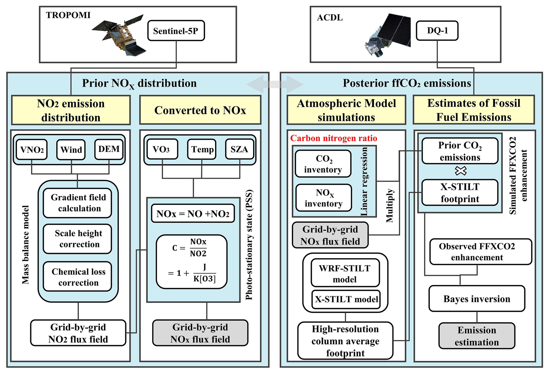
In this study, we propose a city-scale ffCO₂ inversion framework that jointly assimilates active and passive satellite observations, dynamically bridging NO_x and CO₂ emissions via the CO₂-to-NO_x ratio. The workflow is illustrated in Fig. 1. TROPOMI NO₂ column data are first used to invert NO_x gridded emissions via a mass-balance approach. Combined with prior CO₂-to-NO_x ratios, these NO_x fluxes are converted into CO₂ priors. DQ-1 XCO₂-Lidar along-track measurements are then assimilated using WRF-STILT high-resolution atmospheric transport simulations within a Bayesian inversion framework to estimate total city emissions and explicitly quantify observational and transport uncertainties. We applied this approach to Beijing, Paris, and Cairo, representing cities with diverse topographies and emission patterns, using August 2022 TROPOMI and DQ-1/ACDL data to evaluate the framework's ability to provide robust, high-resolution urban emission estimates. It is noteworthy that no unified CO₂-to-NO_x ratio calculation method currently exists, and different methods yield divergent values, which can significantly bias final emission estimates. This study systematically evaluates the influence of prior CO₂-to-NO_x ratio calculation methods on inversion outcomes, demonstrating that Bayesian assimilation can substantially reduce this uncertainty, converging different ratios to a consistent magnitude. This framework offers a unified approach for estimating urban emissions under limited or uncertain inventory conditions, providing a timely and reliable method for reporting anthropogenic CO₂ emissions at the city scale.

Figure 1 Technical framework diagram.

The remainder of this paper is structured as follows. Section 2 introduces the datasets and methods used in this study. Section 3 presents the results of NO_x emission estimation in Paris, Cairo, and Beijing based on TROPOMI observations combined with a mass-balance approach, followed by city-scale ffCO₂ inversion results obtained by assimilating DQ-1 ACDL observations within a Bayesian framework. Section 4 examines the influence of different prior CO₂-to-NO_x ratio calculation methods on the inversion process and highlights the importance of optimizing the CO₂-to-NO_x ratio using observational data. Finally, Sect. 5 summarizes and discusses the potential of the multi-source satellite Bayesian inversion framework for constraining urban CO₂ emissions, and emphasizes the significance of optimized CO₂-to-NO_x ratios for improving the accuracy of urban ffCO₂ estimates.

2 Materials and methods

2.1 Data

2.1.1 ACDL Productions

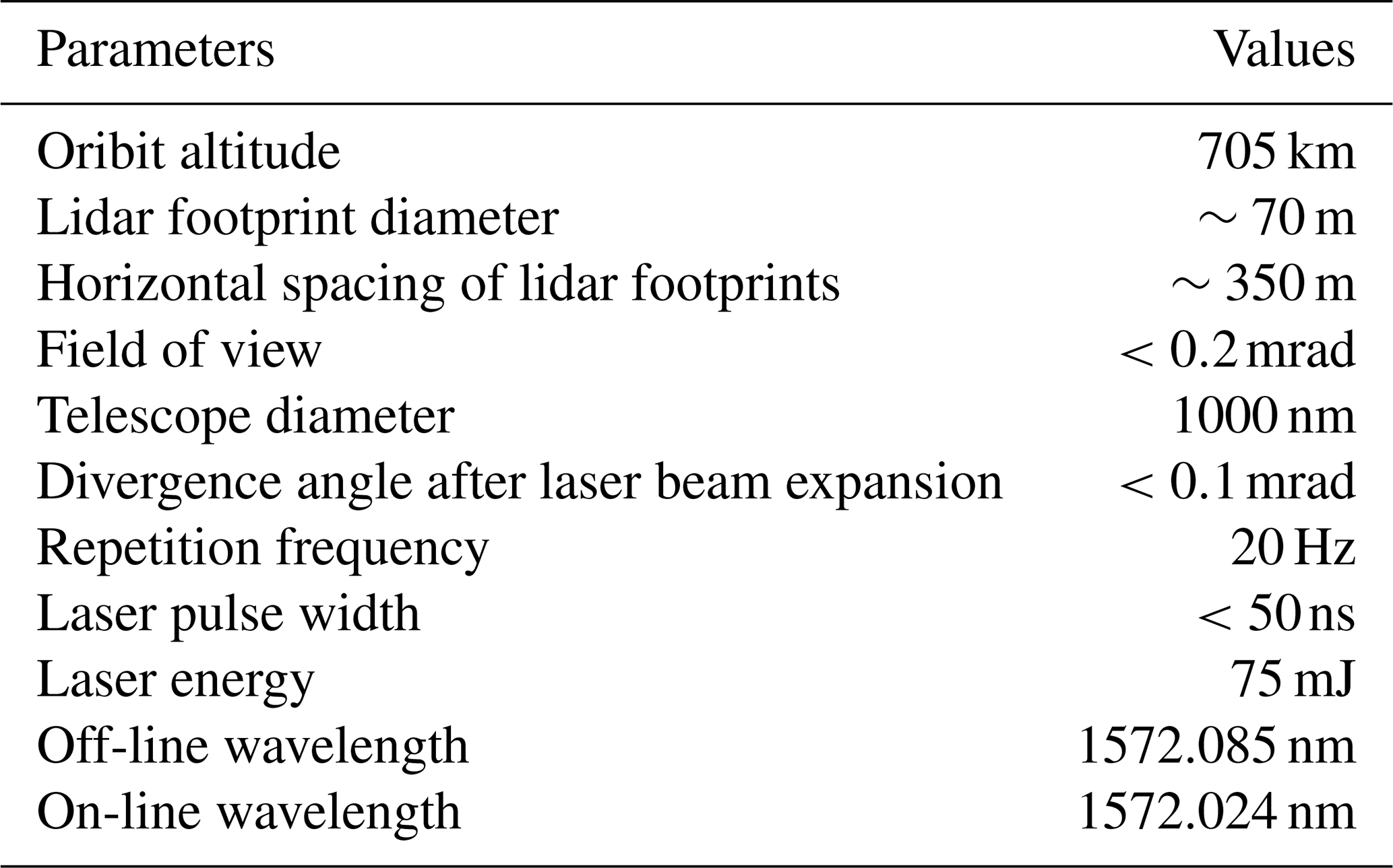
The concept of DQ-1 was first proposed in 2012 with the aim of developing a satellite-borne lidar system analogous to the Cloud-Aerosol Lidar with Orthogonal Polarization (CALIOP) onboard CALIPSO, and it was officially approved as a national project in 2017 (Zhang et al., 2024). Unlike conventional environmental monitoring satellites, DQ-1 is distinguished by its breakthrough active remote sensing payload – the Atmospheric Carbon Dioxide Differential Absorption Lidar (ACDL) – which enables active “top-down” observations of atmospheric CO₂ (Zhang et al., 2023). The ACDL underwent successive stages of laboratory prototype development and airborne validation before its successful launch onboard the DQ-1 satellite into a near-polar sun-synchronous orbit at an altitude of ∼705 km on 18 April 2022. Operational observations commenced in late May of the same year. This study primarily analyzes data collected August 2022.

The ACDL operates on the principle of Integrated Path Differential Absorption (IPDA) lidar, retrieving atmospheric column-averaged CO₂ concentrations (XCO₂) via differential absorption techniques. The inversion methodology and data product specifications have been described in detail elsewhere; here, we provide only a brief overview (Han et al., 2025). The instrument transmits two nearly simultaneous laser pulses: one at a strong absorption line of CO₂ (R16, referred to as the “online” wavelength) and the other at a nearby weak absorption line (the “offline” wavelength). These are stabilized at 6361.225 and 6360.981 cm⁻¹, corresponding to 1572.024 and 1572.085 nm, respectively. By comparing the differential attenuation between the online and offline signals, the system effectively mitigates the influence of aerosols and other interfering species, except water vapor, thereby enabling accurate retrievals of XCO₂. The inversion process relies on dedicated algorithms, with the central concept being that the small wavelength offset produces differential absorption, which enhances the sensitivity of CO₂ detection (details of the ACDL XCO₂ retrieval algorithm are provided in the Appendix A1).

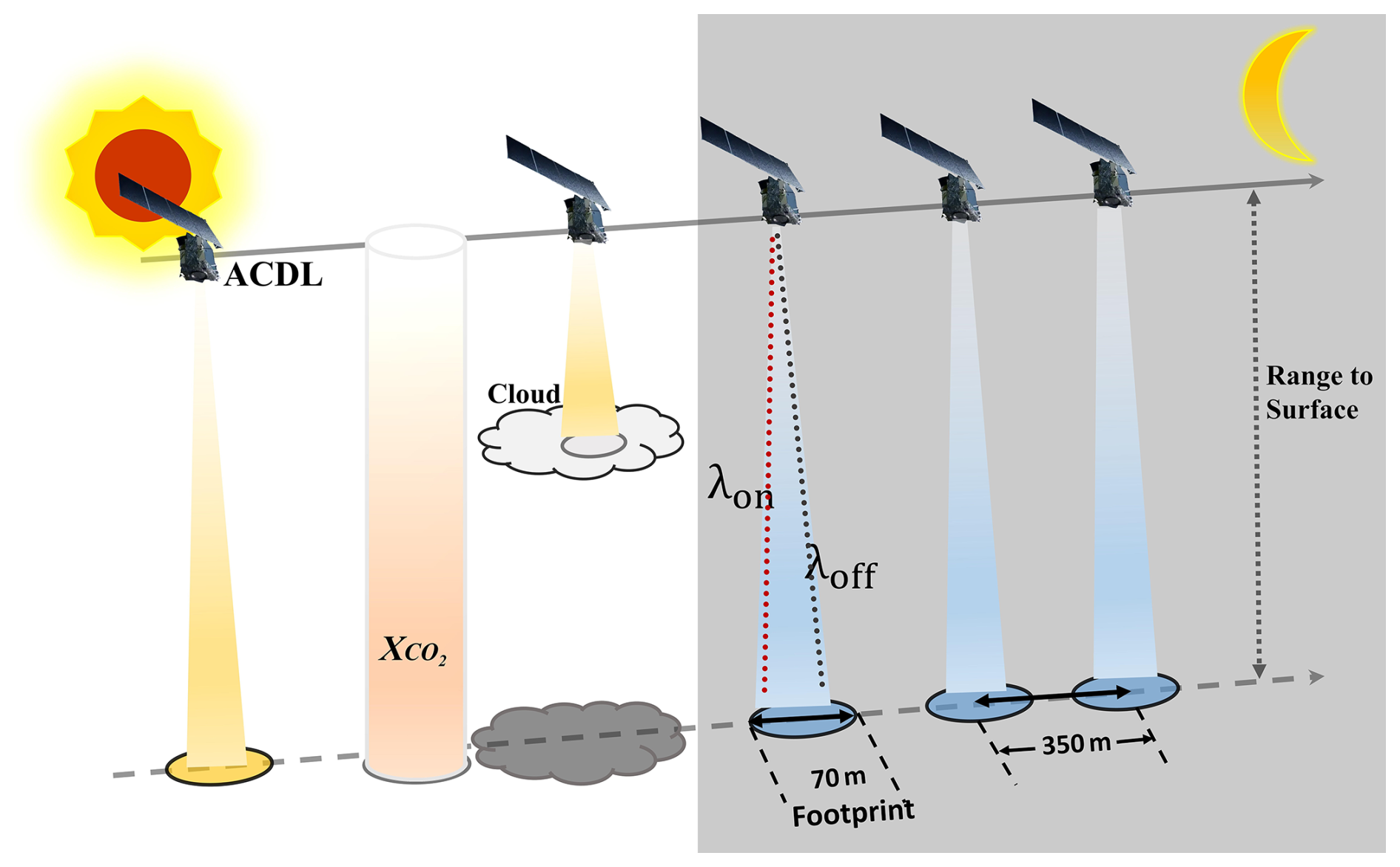
Figure 2 illustrates the schematic of the DQ-1 measurement principle. The XCO₂ products generated by ACDL are provided in a point-sampling mode analogous to that of GOSAT. The lidar records one footprint of approximately 70 m every ∼350 m along the satellite ground track. Additional details of the ACDL operating parameters are provided in the Appendix A1.

Figure 2 the schematic diagram for DQ-1's detection principle.

2.1.2 TROPOMI Productions

TROPOMI is a nadir-viewing spectrometer onboard ESA's Sentinel-5 Precursor (S5P) satellite, which was launched in October 2017. Operating in an ascending Sun-synchronous polar orbit with an equator crossing time of approximately 13:30 local time, TROPOMI measures a range of trace gases as well as cloud and aerosol properties across four spectral channels (ultraviolet, visible, near-infrared, and shortwave infrared). The instrument's minimum pixel size was about 3.5×7 km² at nadir before being reduced to $\sim \mathrm{3.5}\times \mathrm{5.5}{\mathrm{km}}^{\mathrm{2}}$ on 6 August 2019 (Veefkind et al., 2012). In this study, we used the S5P-PAL dataset (consistent with version 2.3.1) covering the period from 1 August–1 September 2022, obtained from https://data-portal.s5p-pal.com (last access: 29 January 2026).

To ensure data quality, we filtered out pixels with a qa_value<0.75 (Qin et al., 2023), and, following van Geffen et al., removed cloudy pixels (cloud radiance fraction>50 %) as well as anomalies (e.g., eclipses) from the TROPOMI NO₂ dataset (Van Geffen et al., 2022). To test our algorithm framework on a robust dataset, we selected summer NO₂ observations for three cities located in the mid-latitudes of the Northern Hemisphere, avoiding winter measurements that may be complicated by potential snow cover. Furthermore, given the need for city-scale accuracy, air mass factor (AMF) corrections were applied locally following the method described in Beirle et al. (2023).

Sun et al. proposed an oversampling algorithm to project multi-satellite, multi-species observations onto a common grid, with code publicly available on GitHub (https://github.com/Kang-Sun-CfA/Oversampling_matlab/, last access: 29 January 2026) (Sun et al., 2018a). In this work, we applied this algorithm to the pre-processed TROPOMI overpass data, generating oversampled grids at 1 km resolution following the procedure described in Sun (2022).

2.1.3 Meteorological and DEM data

For the estimation of CO₂ emissions through model simulations, we utilized meteorological parameters from the National Centers for Environmental Prediction Final (NCEP FNL) operational global analysis dataset. The ds083.3 dataset is provided on a 0.25°×0.25° latitude–longitude grid and updated every six hours via the Global Data Assimilation System (GDAS) (https://rda.ucar.edu/datasets/ds083-3/, last access: 29 January 2026). It covers 32 vertical levels, ranging from the surface to the top of the atmosphere, including the ground level and 31 isobaric layers from 1000–1 hPa. Essential variables such as surface pressure, geopotential height, temperature, relative humidity, and zonal and meridional wind components were used as the main meteorological inputs for driving the WRF-STILT simulations.

The wind vector data were obtained from the ERA5 reanalysis dataset (https://doi.org/10.24381/cds.adbb2d47) (Hersbach et al., 2023). We extracted hourly 10 and 100 m wind vectors at 0.25° spatial resolution for the three selected cities during the period from 1 August–1 September 2022. The 10 m wind vectors are used to approximate near-surface winds, whereas the 100 m wind vectors represent horizontal transport within the planetary boundary layer. These data were averaged to daily values and subsequently interpolated to match the grid resolution of the column concentration fields described in Sect. 2.3.1.

Digital elevation data were obtained from the GMTED2010 dataset (https://www.usgs.gov/coastal-changes-and-impacts/gmted2010, last access: 29 January 2026) (Danielson and Gesch, 2011). The DEM was resampled and mapped to the same spatial grid as the concentration and wind fields to ensure consistency across all datasets.

2.1.4 Emissions Inventory

In this study, multiple emission inventories were used to estimate fossil fuel CO₂ (ffCO₂) emissions and to calculate the CO₂-to-NO_x ratio. In the urban observation system simulation experiment (Sect. 3), the GEMS inventory (0.1° resolution) for NO_x and CO₂ emissions (Huang et al., 2017) was used to derive the prior CO₂-to-NO_x ratio (available at: https://gems.sustech.edu.cn/data, last access: 29 January 2026). For comparison, we also employed the gridded fossil fuel CO₂ emissions inventory from the Open-source Data Inventory for Atmospheric Carbon dioxide (ODIAC, Version 2024, 1 km resolution; https://db.cger.nies.go.jp/dataset/ODIAC/, last access: 29 January 2026). In Sect. 4, we further utilized the sectoral and 0.1° gridded NO_x and CO₂ inventories from the Emissions Database for Global Atmospheric Research (EDGAR; https://edgar.jrc.ec.europa.eu/emissions_data_and_maps, last access: 29 January 2026) (Crippa et al., 2018), as well as the sectoral NO_x and CO₂ inventories from the Multi-resolution Emission Inventory model for Climate and air pollution research (MEIC; http://meicmodel.org.cn/, last access: 29 January 2026) (Team, 2012). Using different approaches to calculate the CO₂-to-NO_x ratio, we quantified the variations arising from different inventory inputs and assessed their impact on emission inversions.

2.2 Methodology

2.2.1 Calculation of Prior Distribution for CO₂ Emissions

(1) Mass Balance Method

In previous studies, numerous works have detailed the theoretical derivation for inferring gridded fluxes from column observations (Huang et al., 2024; Koene et al., 2024; Qin et al., 2023; Rey-Pommier et al., 2025; Sun, 2022). Such frameworks are generally based on solutions to the atmospheric continuity equation. Divergence-based approaches typically rely on several key assumptions: (1) exchanges above the planetary boundary layer (column top) and at the surface (column bottom) are neglected, effectively assuming two-dimensional diffusion; (2) horizontal turbulent transport is ignored at coarse grid resolutions; and (3) the deposition term S is treated using a first-order chemical approximation. Starting from the unsteady, source-driven atmospheric continuity equation, the gridded flux of a given species, such as NO₂, can be derived from satellite column observations, with the resulting flux $\langle E_{{\mathrm{NO}}_{\mathrm{2}}}\rangle$ expressed as in Eq. (1).

$$\begin{array}{}\text{(1)}& \begin{array}{rl}{\displaystyle }\langle E_{{\mathrm{NO}}_{\mathrm{2}}}\rangle & {\displaystyle }=\langle \mathit{u}\times \left(\mathrm{\nabla }{V}_{{\mathrm{NO}}_{\mathrm{2}}}\right)\rangle {\displaystyle \frac{\langle V_{{\mathrm{NO}}_{\mathrm{2}}}{\mathit{u}}_{\mathrm{10}}\times \left(\mathrm{\nabla }{z}_{\mathrm{0}}\right)\rangle }{H}}\\ {\displaystyle }& {\displaystyle }+{\displaystyle \frac{\langle V_{{\mathrm{NO}}_{\mathrm{2}}}\rangle }{\mathit{\tau }}}\end{array}\end{array}$$

The detailed derivation is provided in Appendix A2. To fully exploit the available data while accounting for observational errors, spatial gradients were computed along the zonal, meridional, and both diagonal directions. Gradients were numerically approximated using second-order central differences, multiplied by the corresponding decomposed wind vectors, and then averaged. For boundary grid points, one-sided differences were applied. Although using gradients in multiple directions helps reduce directional dependence, the finite-difference gradient operator can amplify high-frequency retrieval noise in the original NO₂ column field. Therefore, the divergence-derived NO_x fluxes should not be interpreted as purely deterministic grid-cell emissions. Instead, they represent monthly aggregated estimates subject to retrieval noise, wind-field uncertainty, chemical-parameter uncertainty, and possible structured errors introduced by gradient operations and gridding. We further evaluate this sensitivity in Appendix A5.

(2) Convert NO₂ to NO_x

Nitrogen oxides (${\mathrm{NO}}_x=\mathrm{NO}+{\mathrm{NO}}_{\mathrm{2}}$) do not exist independently in the troposphere, as NO and NO₂ continuously interconvert, while the total NO_x remains relatively stable. To convert between NO₂ column densities and total NO_x columns, Sun et al. (2018a) applied a fixed coefficient of 1.32. In this study, we adopt a more rigorous approach to derive the conversion factor, as expressed in Eq. (2) (Beirle et al., 2023), based on the photostationary steady-state assumption:

$$\begin{array}{}\text{(2)}& \left\{\begin{array}{l}{V}_{{\mathrm{NO}}_x}=\mathit{\alpha }{V}_{{\mathrm{NO}}_{\mathrm{2}}}=\left(\mathrm{1}+{\displaystyle \frac{J}{K{X}_{{\mathrm{O}}_{\mathrm{3}}}}}\right)V_{{\mathrm{NO}}_{\mathrm{2}}}\\ J=k_{\mathrm{1}}\times \exp \left(-{\displaystyle \frac{k_{\mathrm{2}}}{\cos \left(\text{SZA}\right)}}\right)\\ K=k_{\mathrm{3}}\times \exp \left(-{\displaystyle \frac{k_{\mathrm{4}}}{T}}\right)\end{array}\right.\end{array}$$

here, J represents the photolysis frequency of NO₂, calculated following the methodology in Dickerson et al. (1982). The rate constants k₁ and k₂ are set to 0.0167 and 0.575, respectively. The solar zenith angle (SZA) can be directly determined from the local latitude, longitude, and time; in this study, SZA values are obtained from the TROPOMI satellite metadata. K denotes the chemical reaction rate constants for NO with O₃, expressed in cm³ (mol s)⁻¹ and recommended by IUPAC, with $k_{\mathrm{3}}=\mathrm{2.07}\times \mathrm{10}-\mathrm{12}$ and k₄=1400. The ozone mixing ratio, $X_{{\mathrm{O}}_{\mathrm{3}}}$, is derived from the ESCiMo project (Jöckel et al., 2016), and T represents the boundary-layer mean temperature obtained from ERA5 reanalysis data. Under these definitions, Eq. (2) can be rewritten as:

$$\begin{array}{}\text{(3)}& X=\mathit{\alpha }\times \langle E_{{\mathrm{NO}}_{\mathrm{2}}}\rangle \end{array}$$

Using Eq. (3) we can obtain grid-resolved estimates of NO_x fluxes, which serve as the prior distribution for fossil fuel CO₂ (ffCO₂) emissions. These estimates provide a data-driven prior inventory for subsequent steps in the inversion framework.

(3) Scale height and Chemical lifetime

Regarding the selection of scale height and first-order chemical lifetime, previous studies, such as Beirle et al., employed fixed empirical scale height values and adjusted terrain correction terms to obtain optimal estimates (Beirle et al., 2023). Their chemical lifetime was calculated using a compensation method that accounted for losses integrated over residence times within a 15 km buffer. While effective at point-source scales, this approach is not directly applicable to our study. In the present work, we follow Sun et al.'s (2018b) purely data-driven approach, which leverages observational data without introducing additional assumptions, constructing a linear regression model to determine these parameters (Sun, 2022). This observation-driven fitting method not only reduces errors arising from new assumptions but also mitigates biases caused by grid resampling and near-surface wind selection.

To suppress excessive noise in single-day fits, we perform monthly regressions and adopt the temporal and spatial mean over the month as the final estimate, representing an aggregate over the full spatial domain, the entire month, and the troposphere. The retrieved scale height and first-order chemical lifetime are then applied back into Eqs. (4) and (6) to obtain the final gridded NO_x vertical fluxes.

After terrain correction, the gridded flux fields remove a substantial portion of strong emission signals obscured by wind divergence and negative divergence artifacts, while the chemical correction term adjusts residual minor negative biases (Sun, 2022; Beirle et al., 2023). Any remaining small negative values after these corrections are set to zero.

(4) Calculation of Prior CO₂-to-NO_x Ratio

We used the prior CO₂-to-NO_x ratio in combination with TROPOMI-derived NO_x emission distributions to obtain an initial characterization of urban prior ffCO₂ emissions. Following the approach of Feng et al. (2024), who calculated the CO₂-to-NO_x ratio by dividing gridded CO₂ and NO_x emission inventories, we derived city-specific prior CO₂-to-NO_x ratio using the 0.1° CO₂ and NO_x inventories from GEMS (https://gems.sustech.edu.cn/data/database, last access: 29 January 2026). Unlike Feng et al. (2024), who focused on grid-level CO₂-to-NO_x ratio, we fitted the gridded ratios across each study region to obtain an integrated city-level CO₂-to-NO_x ratio, which is more suitable for subsequent inversion analyses (Fig. 3). Details on the associated uncertainties are provided in Sect. 4.1.

Figure 3 illustrates our method for calculating the prior CO₂-to-NO_x ratio. By fitting the 0.1° gridded ratios for each city, we obtained overall city-scale values. The coefficients of determination (R²) for Paris, Cairo, and Beijing were 0.96, 0.917, and 0.76, respectively.

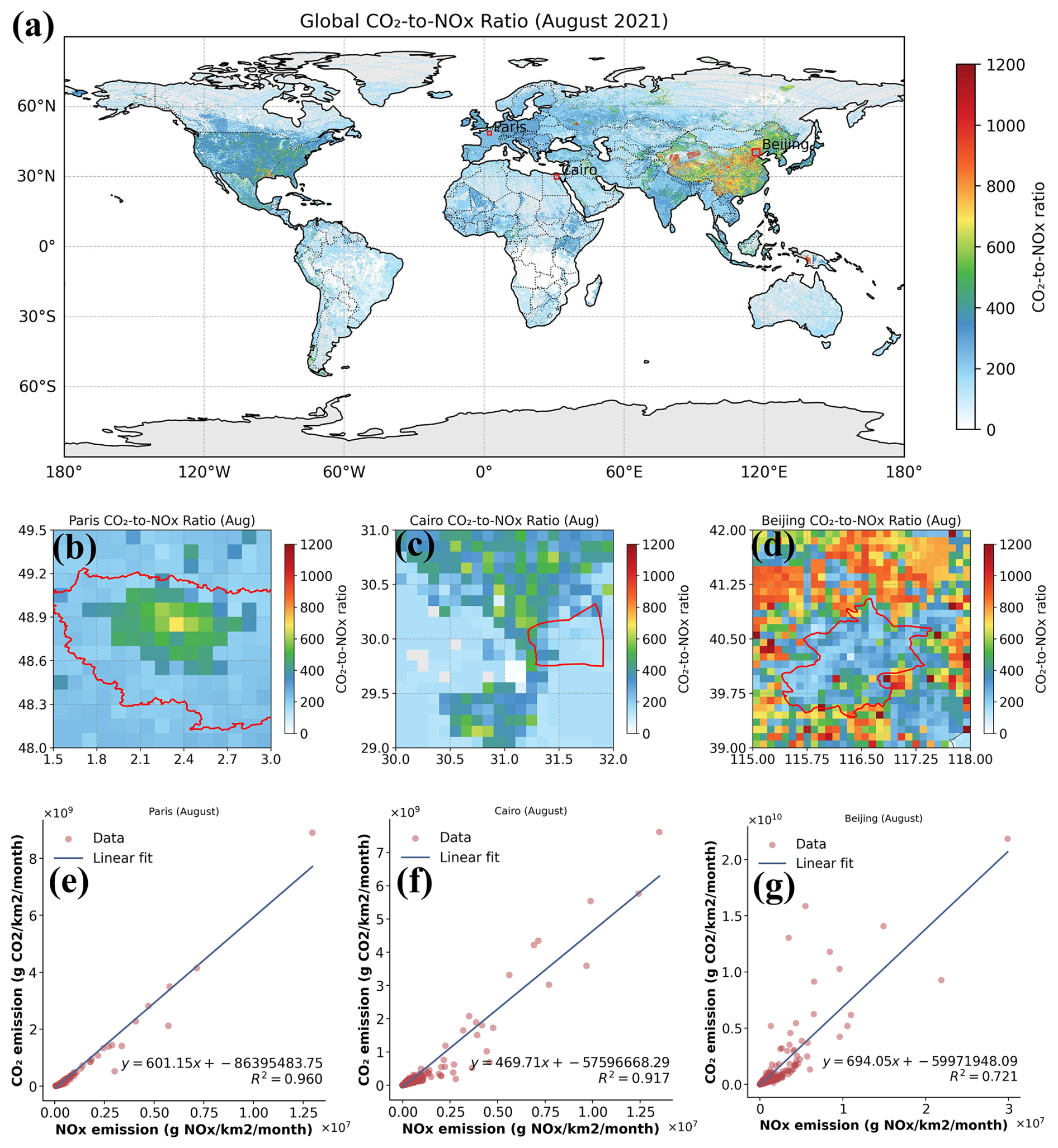
Figure 3 Schematic diagram of prior CO₂-to-NO_x ratio calculation methods. Panel (a) shows the global gridded CO₂-to-NO_x ratio derived from GMES data. Panels (b)–(d) present the gridded CO₂-to-NO_x ratio for Paris, Cairo, and Beijing (the red lines indicate the boundaries of each city). Panels (e)–(g) display the overall CO₂-to-NO_x ratio fitting results for the three cities. We used the Île-de-France administrative boundary to depict Paris in the figures, rather than the city proper. Although our actual study area only covers a subset of Île-de-France (1.5–3° E, 48–49.5° N)

Recently, an increasing number of studies have employed NO_x emissions to estimate ffCO₂ emissions (Feng et al., 2024; Zheng et al., 2020; Xu et al., 2025b; Yang et al., 2023; Zhang et al., 2022). In inversion methods based on NO_x emissions, the choice of the prior CO₂-to-NO_x ratio directly affects the emission estimates. Uncertainty in the prior ratio propagates to the estimated ffCO₂ emissions, influencing both their magnitude and spatial distribution. To evaluate this effect, we selected several widely used CO₂-to-NO_x ratio calculation methods and systematically assessed their associated uncertainties (results see Sect. 4.1 and Appendix A6).

• M.1 Grid-level CO₂-to-NO_x ratio derived directly from gridded CO₂ and NO_x inventories (Feng et al., 2024). Since this study scales emissions to the city level, we further fitted the grid-level ratios to obtain city-integrated CO₂-to-NO_x ratios. M.1 calculations were based on the GEMS gridded inventory.

• M.2 CO₂-to-NO_x ratios calculated using sectoral emission factors for CO₂ and NO_x(Zheng et al., 2020). We derived city-scale ratios by aggregating across all sectors. M.2 used the GEMS sectoral emission factors.

• M.3 CO₂-to-NO_x ratios derived from near-real-time satellite observations. Background-stable NO_x plumes were used to constrain CO₂ plumes, and joint fitting of the two concentrations was performed using the cross-sectional flux method (Xu et al., 2025b; Reuter et al., 2019). The CO₂-to-NO_x ratio was obtained directly from the half-width at half-maximum. Following this approach, we used TROPOMI and OCO-2 observations to calculate city-scale ratios.

• M.4 Same as M.2, but the MEIC sectoral inventory was used for Beijing.

• M.5 Same as M.1, but calculations were based on the EDGAR gridded inventory.

• M.6 Same as M.2, but calculations were based on the EDGAR sectoral inventory.

2.2.2 Estimating ffCO₂ emissions by WRF-STILT simulations

(1) Quantifying ffXCO₂ enhancements

Distinguishing anthropogenic emission signals from the surrounding “clean” background in XCO₂ observations is a central challenge for constraining urban carbon emissions via satellite. Definitions of “background” vary across studies. In this work, we define the background as atmospheric XCO₂ that is unaffected by local emissions within the study region. Following the approach proposed by Ye et al. (2020) in constraining urban emissions using OCO-2 observations, we adopt a baseline calculation strategy that incorporates latitudinal gradients.

In this framework, XCO₂ is decomposed into two components: ${X{\mathrm{CO}}_{\mathrm{2}}}_{\text{trend}}$, representing the regional-scale, non-local trend, and ${X{\mathrm{CO}}_{\mathrm{2}}}_{\text{local}}$, whose standard deviation σ_local characterizes local-scale variability. Samples satisfying $X{\mathrm{CO}}_{\mathrm{2}}<{X{\mathrm{CO}}_{\mathrm{2}}}_{\text{trend}}+\mathrm{0.5}{\mathit{\sigma }}_{\text{local}}$ are selected as “background samples,” as they exhibit lower local spatial variability compared with data influenced by fossil fuel emissions. These background samples are then subjected to linear regression to derive the background baseline and characterize its spatial variation.

(2) X-Stochastic Time-Inverted Lagrangian Transport model for ACDL productions

We employ the X-STILT V1 model to trace CO₂ concentration variations driven by prior emission information. X-STILT integrates satellite profile data and enables a comprehensive uncertainty assessment of urban XCO₂ enhancements on a per-observation basis (Wu et al., 2018). Originally developed to extract urban signals from passive OCO-2 XCO₂ observations, we have adapted the framework for use with the active CO₂ satellite DQ-1, with appropriate modifications. The relationship between ${X{\mathrm{CO}}_{\mathrm{2}}}^{\text{Lidar}}$ (DQ-1 XCO₂ observations) measurements and the CO₂ vertical profile, CO₂(p), can be formulated as follows:

$$\begin{array}{}\text{(4)}& \begin{array}{rl}{\displaystyle }{X{\mathrm{CO}}_{\mathrm{2}}}^{\text{Lidar}}& {\displaystyle }={\displaystyle \frac{{\int }_{\text{p\_surface}}^{\text{p\_toa}{\mathrm{CO}}_{\mathrm{2}}\left(p\right)\text{WF(p)}}}{{\int }_{\text{p\_surface}}^{\text{p\_toa}}\text{WF(p)}\mathrm{d}p}}\\ {\displaystyle }& {\displaystyle }={\sum }_{n=\mathrm{1}}^{\text{toa}}{\displaystyle \frac{\text{WF}\left(p_n\right)}{\text{IWF}}}\times {\mathrm{CO}}_{\mathrm{2}}\left(p_n\right)\end{array}\end{array}$$

here, p_toa represents the pressure at the bottom height of the ACDL, and p_surface represents the pressure corresponding to the surface elevation at the laser footprint. WF and IWF denote the weighting function and the normalized weighting function of the ACDL, respectively. A detailed description is provided in Appendix A1.

We approximate the CO₂ concentration by summing the background concentration with the simulated ffCO₂ enhancement. Here, the simulated ffCO₂ enhancement, $\mathrm{\Delta }{{\mathrm{CO}}_{\mathrm{2}}}_{{\mathrm{ffCO}}_{\mathrm{2}}}\left(p\right)=\langle {\mathrm{ffCO}}_{\mathrm{2}},\text{foot}\left(p\right)\rangle$, is obtained by interpolating the modeled ffCO₂ fluxes along tracer-tagged footprints. Consequently, the relationship between the ffCO₂ fluxes and the simulated ${X{\mathrm{CO}}_{\mathrm{2}}}_{\text{mod}}^{\text{Lidar}}$, is established, yielding the modeled fossil fuel CO₂ enhancement ${X{\mathrm{CO}}_{\mathrm{2}}}_{{\mathrm{ffCO}}_{\mathrm{2}},\text{mod}}^{\text{Lidar}}$ along the lidar track:

$$\begin{array}{}\text{(5)}& \begin{array}{rl}{\displaystyle }& {\displaystyle }{X{\mathrm{CO}}_{\mathrm{2}}}_{{\mathrm{ffCO}}_{\mathrm{2}},\text{mod}}^{\text{Lidar}}={X{\mathrm{CO}}_{\mathrm{2}}}_{\text{mod}}^{\text{Lidar}}-{X{\mathrm{CO}}_{\mathrm{2}}}_{\text{background}}^{\text{Lidar}}\\ {\displaystyle }& {\displaystyle }={\sum }_{n=\mathrm{1}}^{\text{toa}}{\displaystyle \frac{\text{WF}\left(p_n\right)}{\text{IWF}}}\times \langle \text{emissions},\text{foot}\left(p_n\right)\rangle \end{array}\end{array}$$

${X{\mathrm{CO}}_{\mathrm{2}}}_{\text{background}}^{\text{Lidar}}$ represents the background concentration along the selected DQ-1 orbit (see Sect. 2.2.2 (1)). The operator 〈,〉 denotes an inner product, emissions is the prior emission flux, and foot(p_n) represents the modeled footprint at different vertical layers. Using the above formulation, the mathematical foundation for the inversion is established. By integrating footprints across multiple release heights, the equation can be further simplified. In this study, we define the ffXCO₂ enhancement simulated via the atmospheric transport model as:

$$\begin{array}{}\text{(6)}& {\displaystyle }& {\displaystyle }{\text{XSTILT}}^{\text{Lidar}}=\sum _{n=\mathrm{1}}^{\text{toa}}{\displaystyle \frac{\text{WF}\left(p_n\right)}{\text{IWF}}}\times \text{foot}\left(h_n\right)\text{(7)}& {\displaystyle }& {\displaystyle }{X{\mathrm{CO}}_{\mathrm{2}}}_{{\mathrm{ffCO}}_{\mathrm{2}},\text{mod}}^{\text{Lidar}}=\langle {\text{XSTILT}}^{\text{Lidar}},\text{emissions}\rangle \end{array}$$

here, XSTILT^Lidar is defined as the column-averaged footprint, corresponding to the column-averaged CO₂ concentration. The inner product of the column-averaged footprint and the prior emission flux yields the simulated XCO₂ enhancement.

(3) Bayes inversion

We used the NO_x emissions obtained previously as prior fluxes and, through the CO₂-to-NO_x ratio, established the relationship between the prior emissions and the XCO₂ observed by DQ-1 (Eq. 9). The XCO₂ enhancements estimated from DQ-1 observations were then employed to impose “top-down” constraints on the simulated results. Following the approaches of Che et al. (2024); Ye et al. (2020); Sheng et al. (2025), we applied a Bayesian inversion framework to optimize the prior emission estimates.

$$\begin{array}{}\text{(8)}& y_{\text{obs}}=y_{\text{sim}}\times \mathit{\lambda }+{\mathit{\epsilon }}_{\mathrm{p}}\end{array}$$

here, y_obs and y_sim represent the observed ffXCO₂ enhancements and the simulated NO_x enhancements, respectively. The symbol λ denotes the CO₂-to-NO_x ratio, and ε_p represents the observational error, which encompasses contributions from DQ-1 measurement uncertainties, model errors, and errors in model parameters. It is defined as follows:

$$\begin{array}{}\text{(9)}& {\displaystyle }& {\displaystyle }\left\{\begin{array}{l}{y}_{\text{obs}}={\int }_{\text{latitude1}}^{\text{latitude2}}{\mathrm{ff}X{\mathrm{CO}}_{\mathrm{2}}}_{\text{obs}}\mathrm{d}t\\ y_{\text{sim}}={\int }_{\text{latitude1}}^{\text{latitude2}}\langle X,\text{footprint}\rangle \mathrm{d}t\end{array}\right.\text{(10)}& {\displaystyle }& {\displaystyle }{\mathit{\epsilon }}_{\text{obs}}=\sqrt{{\mathit{\sigma }}_{\text{measurement}}^{\mathrm{2}}+{\mathit{\sigma }}_{\text{sim}}^{\mathrm{2}}}\end{array}$$

In this context, ${\mathrm{ff}X{\mathrm{CO}}_{\mathrm{2}}}_{\text{obs}}$ represents the DQ-1 XCO₂ enhancement after background concentration removal. The notation 〈Xfootprint〉 denotes the simulated NO_x enhancement, obtained by convolving the NO_x emission inventory X with the STILT-derived footprint (It should be noted that the footprints used here represent hourly footprints during the simulation period, whereas the NO_x emissions are monthly emissions derived using the method described in Sect. 2.2.1. Therefore, we use the New High Resolution Temporal Profiles in EDGAR dataset (https://edgar.jrc.ec.europa.eu/dataset_temp_profile, last access: 29 January 2026) to distribute the monthly NO_x emissions to each hourly footprint). Pseudo-observations, ${\mathrm{ff}X{\mathrm{CO}}_{\mathrm{2}}}_{\text{obs}}$, are generated by averaging DQ-1 measurements over one-second intervals along the satellite track (∼7 km), together with the corresponding simulated values.

Following the Bayesian inversion approach, the state vector λ is expressed in terms of the CO₂-to-NO_x ratio, representing the relationship between urban fossil fuel CO₂ and NO_x emissions. The Jacobian matrix is derived from the simulated NO_x enhancement y_sim. Here, ${\mathit{\sigma }}_{\text{measurement}}^{\mathrm{2}}$ represents the observational error variance, and ${\mathit{\sigma }}_{\text{sim}}^{\mathrm{2}}$ denotes the model transport error variance. DQ-1 observations are assumed unbiased with respect to the true state. To account for measurement uncertainty, random Gaussian noise with a standard deviation of 0.3 ppm – representing the lower limit of observational error – is added to the observations.

By minimizing the loss function, we obtain the posterior CO₂-to-NO_x ratio $\widehat{\mathit{\lambda }}$ and posterior uncertainty $\widehat{\mathit{\sigma }}$:

$$\begin{array}{}\text{(11)}& {\displaystyle }& {\displaystyle }\begin{array}{rl}{\displaystyle }\widehat{\mathit{\lambda }}=& {\displaystyle }\mathit{\lambda }+{\mathit{\sigma }}_{\text{sim}}^{\mathrm{2}}{y}_{\text{sim}}^{\mathrm{T}}{\left(y_{\text{sim}}{S}_{\text{obs}}{y}_{\text{sim}}^{\mathrm{T}}+S_{\text{obs}}\right)}^{-\mathrm{1}}\\ {\displaystyle }& {\displaystyle }\times (y_{\text{obs}}-y_{\text{sim}}\mathit{\lambda })\end{array}\text{(12)}& {\displaystyle }& {\displaystyle }{\displaystyle }\widehat{\mathit{\sigma }}{}^{\mathrm{2}}={\left(y_{\text{sim}}^{\mathrm{T}}{S}_{\text{obs}}^{-\mathrm{1}}{y}_{\text{sim}}+{\mathit{\sigma }}_{\text{sim}}^{-\mathrm{2}}\right)}^{-\mathrm{1}}\end{array}$$

here, S_obs is a diagonal matrix, with the diagonal entries representing the observational error variances ${\mathit{\epsilon }}_{\text{obs}}^{\mathrm{2}}$ for each orbit. The prior uncertainty σ_sim is primarily derived from the uncertainties in the prior NO_x emission distribution ${\mathit{\sigma }}_{{\mathrm{NO}}_x}$ and the prior CO₂-to-NO_x ratio ${\mathit{\sigma }}_{\mathrm{C}/\mathrm{N}}$ as Eq. (13):

$$\begin{array}{}\text{(13)}& {\mathit{\sigma }}_{\text{sim}}=\sqrt{{\mathit{\sigma }}_{{\mathrm{NO}}_x}^{\mathrm{2}}+{\mathit{\sigma }}_{\mathrm{C}/\mathrm{N}}^{\mathrm{2}}}\end{array}$$

3 Urban Observation System Simulation Experiment

3.1 Satellite-driven urban NO_x emission distribution

As described in Sect. 2.2.1, we applied the mass balance approach in the three cities to derive prior NO_x gridded inventories, which serve as the basis for constructing ffCO₂ gridded emissions. The grid resolution was set to 5 km×5 km. Figure 4 illustrates the detailed NO_x fluxes for August 2022 over Beijing, Paris, and Cairo, produced entirely via a top-down approach, with panels (a)–(c) corresponding to Beijing, Paris, and Cairo, respectively.

From the figure, it is evident that the average NO_x flux magnitude in all three cities is on the order of $\sim {\mathrm{10}}^{-\mathrm{8}}\mathrm{mol}{\mathrm{m}}^{-\mathrm{2}}{\mathrm{s}}^{-\mathrm{1}}$. However, their spatial distributions differ considerably. Both Paris and Cairo exhibit highly concentrated emission patterns. In Cairo, the central urban area and industrial zones display peak NO_x fluxes on the order of $\sim {\mathrm{10}}^{-\mathrm{7}}\mathrm{mol}{\mathrm{m}}^{-\mathrm{2}}{\mathrm{s}}^{-\mathrm{1}}$. These high-flux regions sharply decrease with distance from the center, highlighting a pronounced urban boundary effect (Li et al., 2025). In contrast, Beijing not only exhibits strong emissions in the central urban area (within the Sixth Ring Road) but also features numerous dispersed point- and area-like sources in suburban districts (e.g., Fangshan in the southwest) and in the surrounding hills and mountains. Compared with Cairo's concentrated emissions, Beijing's peak NO_x grid flux in the urban core is nearly one order of magnitude lower (see the color scale mapping in Fig. 4); however, due to the city's larger spatial extent, the total flux remains substantially higher than that of Cairo.

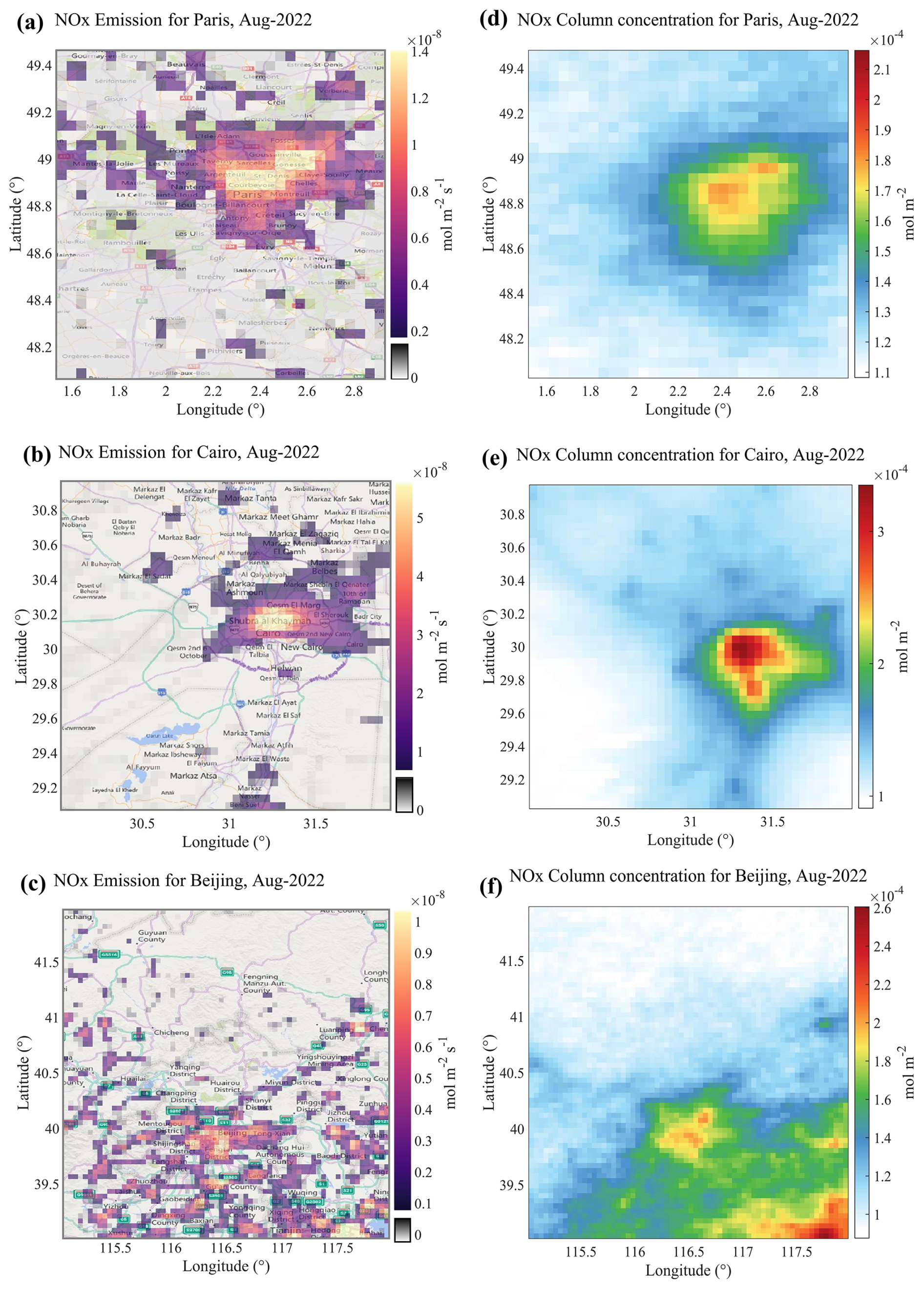
Figure 4 Gridded prior NO_x emission inventories derived from the mass balance method. Panels (a)–c) show the NO_x flux distributions (unit: $\mathrm{mol}{\mathrm{m}}^{-\mathrm{2}}{\mathrm{s}}^{-\mathrm{1}}$) for Beijing, Paris, and Cairo in August 2022. Panels (d)–f) present the resampled monthly mean NO₂ column concentration distributions for the three cities. Basemap for panels (a)–c): Esri World Topographic Map. Sources: Esri, HERE, Garmin, Intermap, INCREMENT P, GEBCO, USGS, FAO, NPS, NRCan, GeoBase, IGN, Kadaster NL, Ordnance Survey, Esri Japan, METI, Mapwithyou, NOSTRA, ©OpenStreetMap contributors, and the GIS user community | Powered by Esri.

Beijing's topography, with higher elevations in the northwest and lower elevations in the southeast, can induce local wind divergence over hilly and mountainous areas. This effect may generate false positives when using the divergence method (Sun et al., 2021; Liu et al., 2021). In the northwestern suburban mountains of Beijing, the mean wind divergence can reach magnitudes of $\sim \pm {\mathrm{10}}^{-\mathrm{4}}{\mathrm{s}}^{-\mathrm{1}}$, while TROPOMI NO₂ column densities are on the order of ${\mathrm{10}}^{-\mathrm{4}}\mathrm{mol}{\mathrm{m}}^{-\mathrm{2}}$. Such magnitudes are comparable to mid-scale urban averages or point-source emissions. Neglecting the divergence term can result in genuine emissions being omitted, while background fluxes induced by terrain or wind divergence are mistakenly included. Following Sun (2022), we applied Eq. (A5) to reconstruct the wind-divergence term using surface wind and terrain gradients, thereby reintegrating previously neglected area-like emissions. Using Beirle et al.'s methodology, we integrated the net gridded fluxes within a 60 km radius centered on Beijing over the entire year of 2022 to estimate the city's annual NO_x emissions at 251 450 t. This value is approximately 9.7 % higher than the 2022 annual emission reported in the MEIC inventory for Beijing (227 000 t). Although the total magnitude is consistent, the spatial distribution from top-down estimates differs substantially from bottom-up inventories. Section 3.2.2 further analyzes these differences by simulating urban ffCO₂ plumes using both our ffCO₂ inventory and the ODIAC inventory.

By comparison, Paris and Cairo are situated on relatively flat terrain (maximum elevation ∼180 m). Terrain-induced wind divergence is negligible relative to total fluxes (wind-terrain and divergence contributions $\sim {\mathrm{10}}^{-\mathrm{10}}\mathrm{mol}{\mathrm{m}}^{-\mathrm{2}}{\mathrm{s}}^{-\mathrm{1}}$), leaving the continuity equation primarily governed by wind-weighted column gradients. Cairo, located upstream of the Nile Delta in a high-albedo desert region, benefits from low uncertainty in satellite-derived NO₂ columns. Under these conditions, the top-down NO_x inventory closely aligns with the bottom-up inventory in terms of spatial distribution. Paris, situated in the Paris Basin along the Seine River, experiences minimal terrain gradients. Although less extreme than Cairo, the slight topographic variation still produces pronounced urban boundary effects in the inversion results.

To quantitatively compare the NO_x emission characteristics and atmospheric behavior among Beijing, Paris, and Cairo, derived using the mass balance approach, we analyzed key parameters for August, including mean NO_x fluxes, total emissions, chemical lifetimes, vertical distribution scale heights, and NO_x$/$NO₂ ratios (Table 1). These NO_x behavior parameters reflect heterogeneous characteristics shaped by the interplay of emission intensity, photochemical conditions, and boundary layer structure.

In terms of mean NO_x flux per unit area ($\mathrm{mol}{\mathrm{m}}^{-\mathrm{2}}{\mathrm{s}}^{-\mathrm{1}}$), Cairo exhibits the highest value ($\mathrm{0.35}\times {\mathrm{10}}^{-\mathrm{8}}$), followed by Paris ($\mathrm{0.28}\times {\mathrm{10}}^{-\mathrm{8}}$) and Beijing ($\mathrm{0.24}\times {\mathrm{10}}^{-\mathrm{8}}$), indicating a higher emission of urban emission sources in Cairo – particularly from traffic – resulting in stronger NO_x release per unit surface area. Nevertheless, Beijing's total NO_x emissions (182 800 t yr⁻¹) are substantially higher than those of the other two cities, reflecting its larger urban extent and greater overall emission intensity, characteristic of a complex multi-source emission profile.

The first-order chemical lifetime of NO_x in the atmosphere indicates its removal rate and is influenced by factors such as OH radical concentration and solar radiation intensity. Paris exhibits the longest NO_x chemical lifetime (6.91 h), followed by Beijing (4.70 h) and Cairo (2.93 h). These differences are closely linked to photochemical activity: strong summer sunlight and high temperatures in Cairo enhance OH-driven removal reactions, whereas the relatively mild mid-latitude climate of Paris, combined with emission control measures, prolongs NO_x lifetime.

Regarding vertical distribution, the NO_x scale height also varies across the three cities. Beijing shows the highest scale height (2.08 km), reflecting the combined effects of strong convective transport and multi-source emissions that elevate NO_x into the upper mixing layer. By contrast, Cairo (1.41 km) and Paris (1.21 km) display more typical boundary-layer-constrained distributions, indicating that ground-level emission controls and thermal structure strongly modulate vertical NO_x transport.

Finally, the NO_x$/$NO₂ ratio provides insight into the proportion of NO and its degree of conversion. Beijing exhibits the highest ratio (1.41), followed by Cairo (1.32) and Paris (1.29), suggesting a higher fraction of NO in Beijing, likely associated with dense traffic sources and a larger fraction of primary NO emissions. The relatively lower ratio in Paris reflects a higher NO₂ fraction, consistent with effective emission controls and extensive photochemical conversion.

Table 1 Grid-averaged NO_x fluxes, with total urban NO_x emissions as intermediate parameters in the mass balance method.

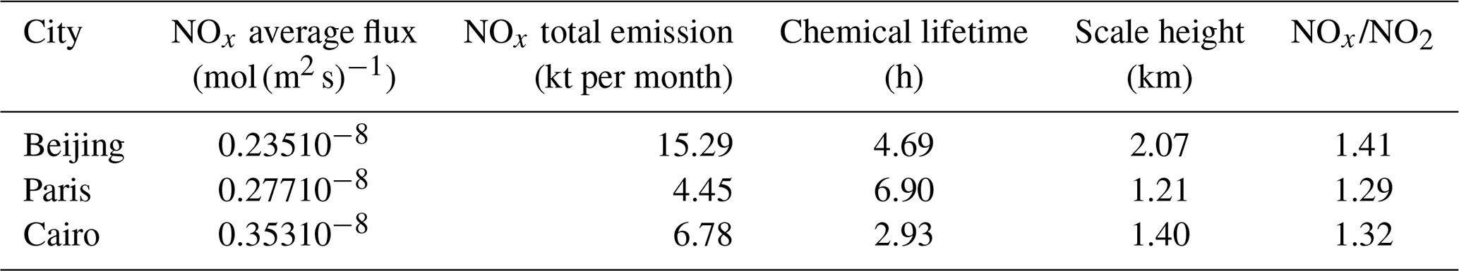
Details of the uncertainties are provided in the Appendix A5.

3.2 Urban Fossil Fuel XCO₂ Enhancement (ffXCO₂)

In this section, we summarize the prior ffXCO₂ emissions for each study region. For the selected orbits, the total monthly emissions of Beijing, Paris, and Cairo were approximately 7.47–9.94, 2.91–3.33, and 2.73–3.60 Mt C per month, respectively. To constrain emissions, we compared observed and simulated ffXCO₂ enhancements, where ffXCO₂ enhancement is defined as the increase in XCO₂ relative to the background level caused by local fossil fuel emissions. The prior ffXCO₂ enhancements were simulated by taking the inner product of prior NO_x emissions inventories with STILT footprints, while the observed enhancements from DQ-1 were derived by subtracting the background concentration from the measured XCO₂. By comparing prior and observed ffXCO₂ enhancements, we assessed the variability of ffXCO₂ along the orbit and investigated the sources and detectability of the ffXCO₂ signal.

3.2.1 Comparison of Modeled and Observed ffXCO₂

Complex horizontal wind fields can lead to elongated and non-Gaussian plume structures in simulated ffXCO₂ distributions (Ye et al., 2020). This feature is illustrated in Fig. 5c–f. Figure 5a and b show the simulated and observed XCO₂ along two overpasses (simulated XCO₂ is obtained by adding the simulated ffXCO₂ to the background derived in Sect. 2.2.2 (1)). Along these overpasses, ffXCO₂ enhancements exceeding 5 and 10 ppm were observed, with the measured enhancements consistently larger than the simulated values. Although the simulated peak on 7 August is narrower than the observed peak, and the observed peak near 48.4° on 21 August shows a ∼0.3° displacement relative to the simulation, the overall magnitude of simulated ffXCO₂ agrees well with observations.

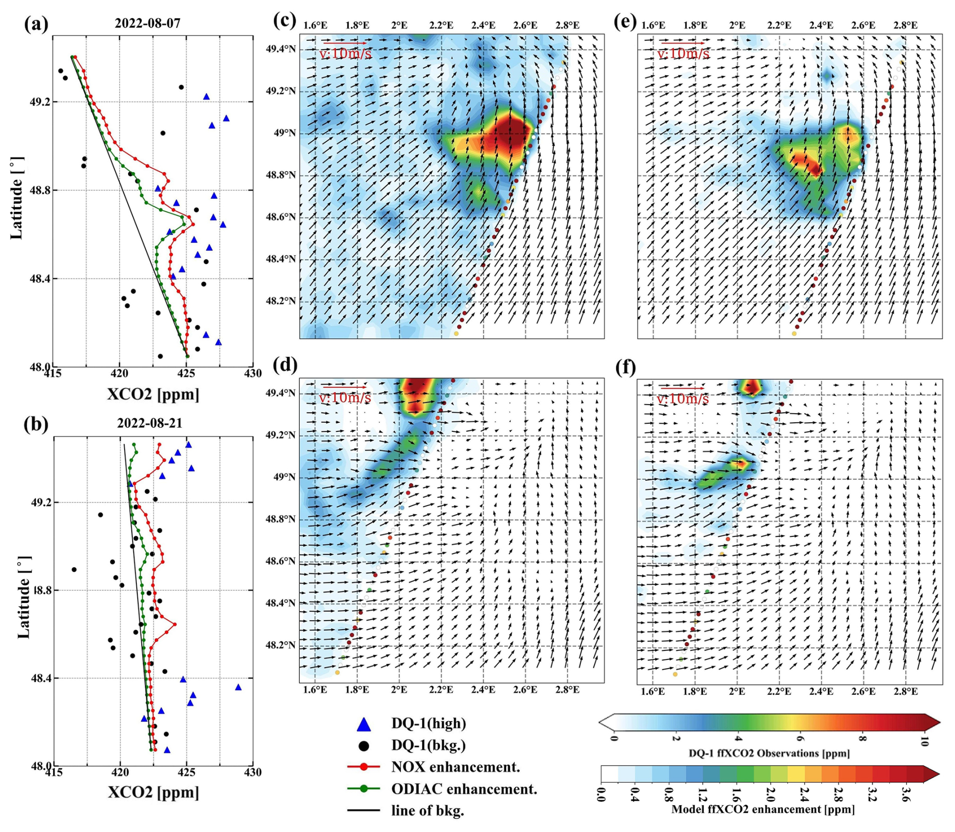
Figure 5 Comparison between simulated and observed ffXCO₂ enhancements using DQ-1 overpasses above Paris on 7 and 21 August 2022 at 01:00 UTC. Panels (a), (b) show DQ-1 XCO₂ along the two tracks (black dots and blue triangles) and simulated XCO₂ (red solid line: sum of background concentration and ffXCO₂ simulated using the NO_x emissions; green solid line: sum of background concentration and ffXCO₂ simulated using the ODIAC inventory), averaged over 0.5 s. Black circles denote the data used to derive the background concentration (black solid line). Panels (c)–f) show simulated ffXCO₂ and observed ffXCO₂ retrieved from DQ-1 data ((c, d): based on the NO_x inventory; (e, f): based on the ODIAC inventory). Background XCO₂ concentrations have been subtracted. The reference vector indicates a wind speed of 10 m s⁻¹.

To further evaluate the feasibility of constraining fossil fuel CO₂ emissions using the NO_x inventory, we performed a comparative analysis using the ODIAC inventory. We compared simulated ffXCO₂ during the satellite overpasses based on the NO_x and ODIAC inventories (colored shaded areas in the figure), as well as their contributions to the pseudo-observed XCO₂ at the satellite locations (colored dots), where the red line represents enhancements derived from the NO_x inventory and the green line represents those from ODIAC. Over Paris, the NO_x-based simulation yields higher ffXCO₂ enhancements than ODIAC, likely due to uncertainty in the prior CO₂-to-NO_x ratio. Nonetheless, both inventories capture enhancements exceeding 4 ppm. Moreover, the line plots indicate that the temporal variation and magnitude of the simulated concentration contributions (red and green lines) are nearly identical.

We examined local ffXCO₂ enhancements during two overpasses of Cairo on 2 August 2022 at 11:00 and 19 August 2022 at 23:00 LT. As shown in Fig. 6, the simulated ffXCO₂ peaks exceed 6 ppm. In contrast to Paris, where enhancements are widespread, diffuse, and lack clear structure, and Beijing, where plumes exhibit complex patterns, the simulated ffXCO₂ over Cairo is strongly influenced by northwesterly winds, resulting in well-defined plumes. Figure 5a illustrates that the simulations based on both inventories on 2 August produce similar magnitudes and trends, consistent with the Paris results, where the NO_x-based simulation exceeds that from ODIAC. Notably, the simulated peaks on 2 August also show a spatial offset relative to the observations. Following Ye et al., 2020, such offsets are attributed to the satellite trajectory crossing the plume edges nearly parallel to the plume axis, making the simulated ffXCO₂ highly sensitive to errors in the horizontal wind field.

Notably, the overpasses above Paris and Cairo (Figs. 5a and 6b) exhibit higher latitudinal gradients in the background XCO₂, as indicated by the background lines. The approach used to derive these background lines provides a reliable estimate of background XCO₂ because, within the relevant regions, the observed and modeled cumulative ffXCO₂ enhancements along the satellite track are largely consistent. Consequently, these findings highlight the effectiveness of the background line method for inferring satellite-observed background XCO₂. They also emphasize that the spatial scale of satellite data analysis is closely linked to the constraints imposed by local emission sources. Neglecting the latitudinal gradient of background XCO₂ may introduce biases in the estimation of ffXCO₂ and, consequently, in derived emission fluxes (Ye et al., 2020).

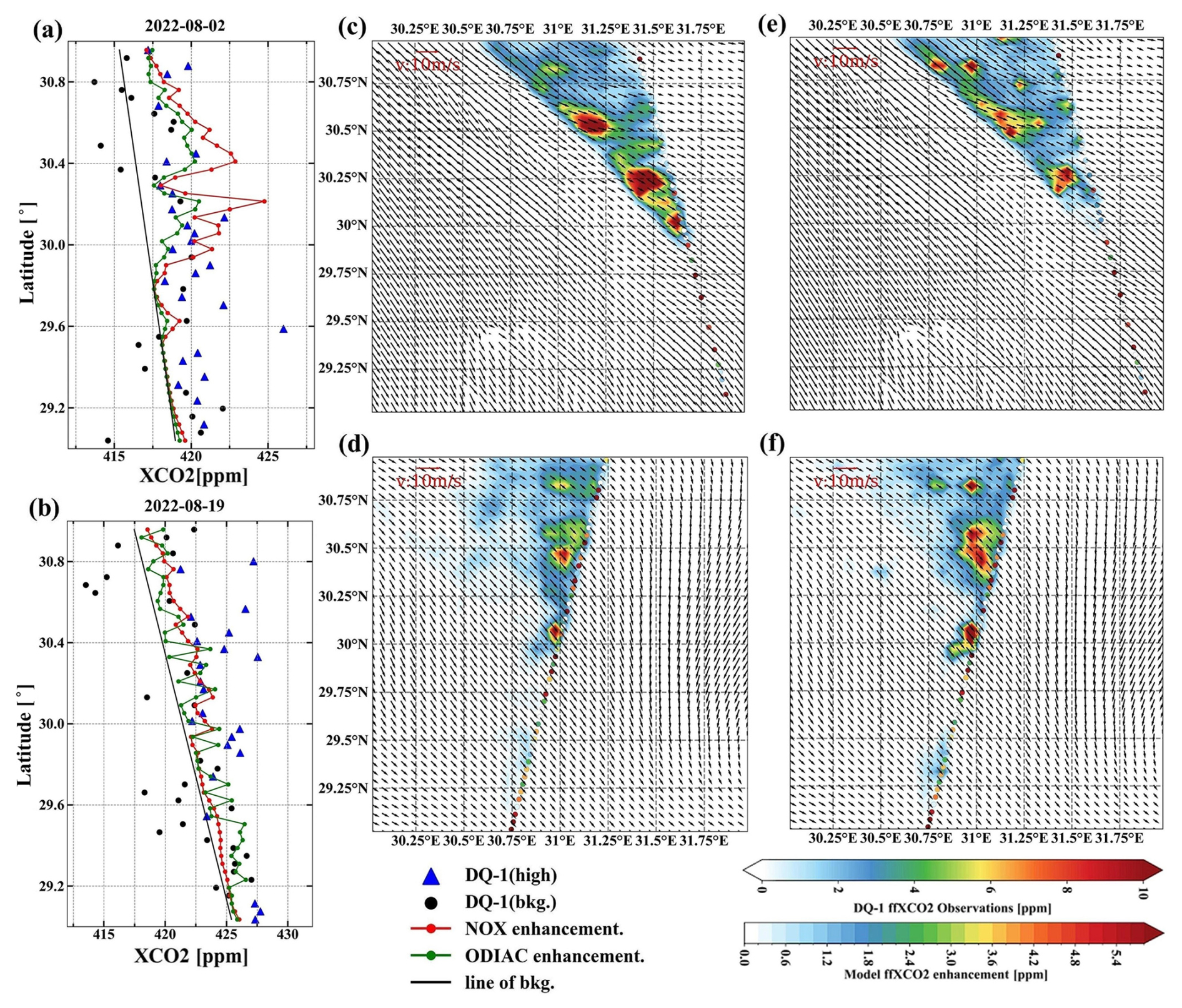
Figure 6 Similar to Fig. 5, comparison between simulated and observed ffXCO₂ enhancements using DQ-1 overpasses above Cairo on 2 August 2022 at 11:00 UTC (a, c, e) and 19 August 2022 at 23:00 UTC (b, d, f). Panels (c), (d) show the simulated ffXCO₂ enhancements based on the NO_x emissions, while panels (e), (f) show those based on the ODIAC inventory.

3.2.2 Comparison of NO_x and ODIAC Modeled ffXCO₂ in Beijing

Figure 7 illustrates the investigation of local ffXCO₂ enhancements over Beijing using two DQ-1 overpasses and corresponding simulated ffXCO₂. In the figure, the colored shading represents XCO₂ concentrations accumulated over the previous 24 h simulated by STILT, while the colored dots indicate satellite-observed XCO₂ enhancements, calculated by subtracting the background values (see Sect. 2.2.2). The red contours outline the urban area of Beijing. As shown, ffXCO₂ over this region can reach approximately 6.0 ppm.

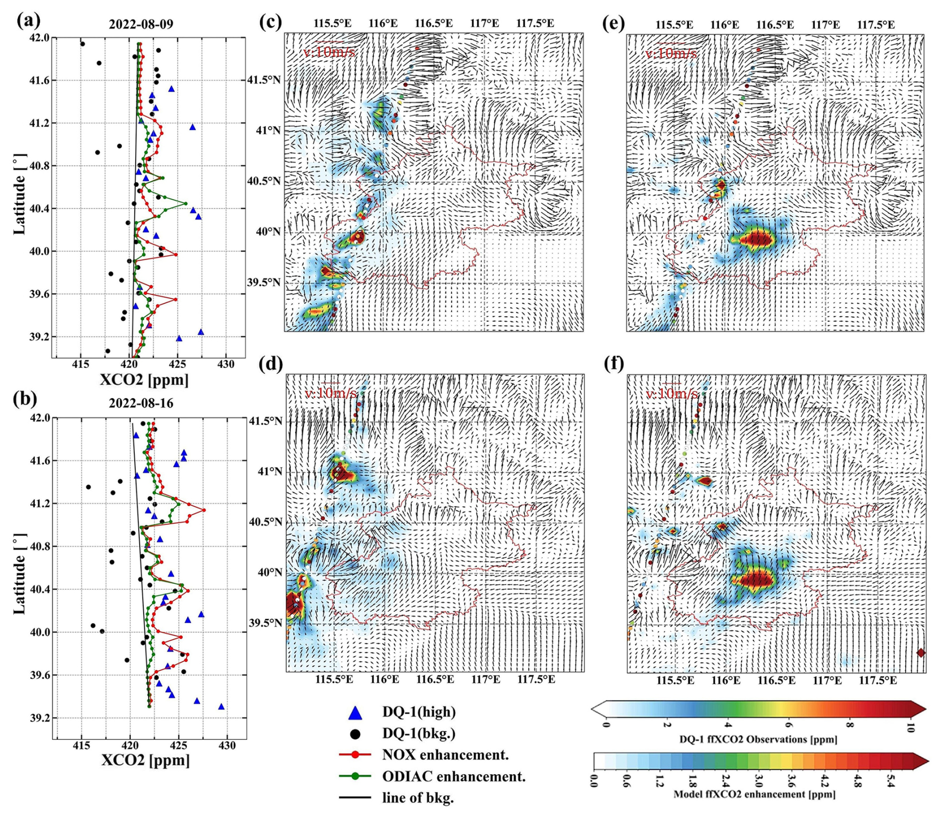
Figure 7 Similar to Fig. 5, comparison between simulated and observed ffXCO₂ enhancements using DQ-1 overpasses above Beijing on 9 August 2022 at 18:00 UTC (a, c, e) and 16 August 2022 at 18:00 UTC (b, d, f). Panels (c), (d) show the simulated ffXCO₂ enhancements based on the NO_x emissions, while panels (e), (f) show those based on the ODIAC inventory.

Notably, simulations based on the NO_x inventory (Fig. 7c and d) show that the spatial distribution of ffXCO₂ enhancements varies significantly with meteorological conditions and emission patterns. In contrast, for Paris and Cairo, the simulated ffXCO₂ is more concentrated. Over Beijing, however, the ffXCO₂ distribution is more dispersed and comprises multiple plumes. When comparing simulations using NO_x and ODIAC inventories for Paris and Cairo, the overall plume structures remain largely unaffected. Over Beijing, the simulations using the ODIAC inventory (Fig. 7e and f) display an almost identical ffXCO₂ enhancement distribution across different wind conditions, showing pronounced anomalies in the urban area. Such similarity is unrealistic.

We attribute this behavior to the ODIAC inventory allocating disproportionately high fossil fuel emissions to central Beijing. When STILT footprints intersect the urban area, the high emission gradients in ODIAC (central urban emissions far exceeding suburban values) amplify ffXCO₂ enhancements in the inner city. ODIAC's low-emission thresholds are influenced by nighttime light saturation, with median differences ranging from 47 %–84 %. Consequently, ODIAC artificially concentrates emissions in the city center while underrepresenting surrounding suburban areas. This makes it challenging to accurately constrain CO₂ fluxes in the peripheral regions using ODIAC. Observations from the TCCON Xianghe site further highlight the limitations of ODIAC's emission allocation in the Beijing area.

Figure 8 presents the comparison of August ffXCO₂ at the TCCON site with simulations using the ODIAC and NO_x inventories. Unlike the ffXCO₂ calculation described in Sect. 2.2.2, the TCCON observations provide daily-averaged fossil fuel CO₂ enhancements, where TCCON ffXCO₂ is calculated as TCCON XCO₂ minus background XCO₂ and NEE contributions (details in the Appendix A3). In Fig. 8a, the dark blue line represents ffXCO₂ simulated at the TCCON site using the NO_x inventory, the green line shows the ffXCO₂ simulated after optimization with the inversion using DQ-1 observations, the light blue line corresponds to ODIAC-based simulations, and the red line depicts TCCON-observed ffXCO₂.

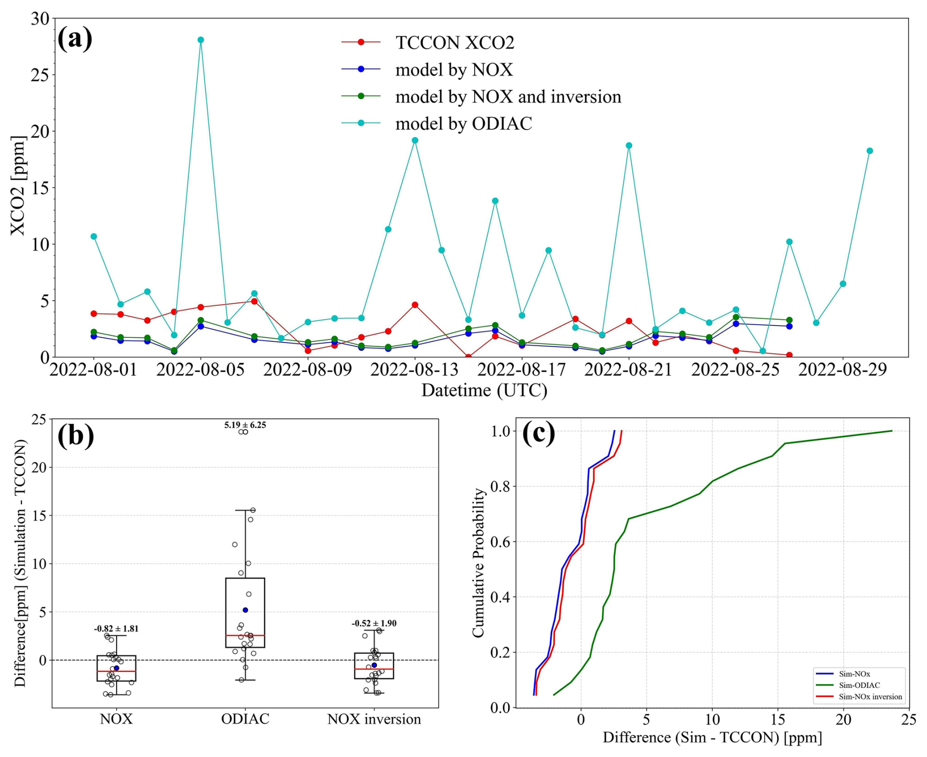
Figure 8 Comparison of ffXCO₂ observed at the TCCON Xianghe site in Beijing during August with ffXCO₂ simulated using the NO_x inventory and the ODIAC inventory. Panel (a) shows the ffXCO₂ observed by TCCON (red line), simulated ffXCO₂ using the NO_x emissions (dark blue line), simulated ffXCO₂ using the ODIAC inventory (light blue line), and simulated ffXCO₂ using the posterior NO_x emissions (green line). Panel (b) presents the distribution of differences between simulated ffXCO₂ (from the NO_x and ODIAC inventories) and TCCON observations throughout August, with bold numbers indicating the mean and standard deviation. Panel (c) shows the cumulative probability distributions of the differences between simulated ffXCO₂ (NO_x emissions and ODIAC inventory) and TCCON observations.

Figure 8b quantifies the accuracy of the simulations by plotting the difference between the simulated ffXCO₂ and TCCON observations on the same day and summarizing the monthly mean and standard deviation. The monthly mean absolute difference for the NO_x inventory is 0.82 ppm, while ODIAC exhibits a much larger discrepancy of 5.19 ppm. The inversion-constrained NO_x inventory reduces the mean absolute difference to 0.52 ppm, closely matching TCCON observations. Figure 8c shows the cumulative probability distribution of the differences between simulated and observed ffXCO₂. The differences for the NO_x and inversion-constrained NO_x simulations are largely centered around zero (blue and red lines), whereas for ODIAC, approximately 30 % of differences exceed 5 ppm.

These results indicate that for Beijing in August, simulations based on the NO_x inventory outperform those using ODIAC. Given that the prior ffCO₂ emissions in both inventories are of similar magnitude, the observed discrepancies are primarily attributable to the spatial allocation of emissions in ODIAC. The combined inversion using TROPOMI and ACDL data provides a more accurate reconstruction of urban ffXCO₂ plume structures.

3.2.3 ffCO₂ Inversion Results

This section presents the inversion results of urban carbon emissions for Cairo, Paris, and Beijing, based on TROPOMI and DQ-1 satellite overpass observations (see Table 2). In the inversion, we systematically accounted for observational errors and uncertainties in atmospheric transport to improve the reliability of the emission estimates. From the posterior results, we derived city-specific CO₂-to-NO_x ratios and, by combining them with TROPOMI-derived NO_x emissions, further quantified fossil fuel CO₂ (ffCO₂) emissions. This approach not only enables quantitative assessment of emissions but also provides a scientific basis for cross-city comparisons of emission characteristics, while demonstrating the potential of multi-satellite data for urban emission monitoring.

Table 2 Results of inversion of for CO₂-to-NO_x ratio selected cities using DQ-1 XCO₂ data.

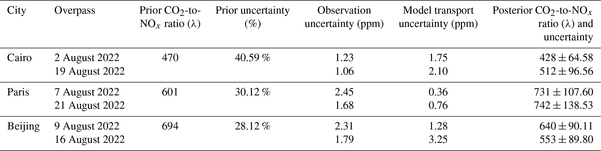
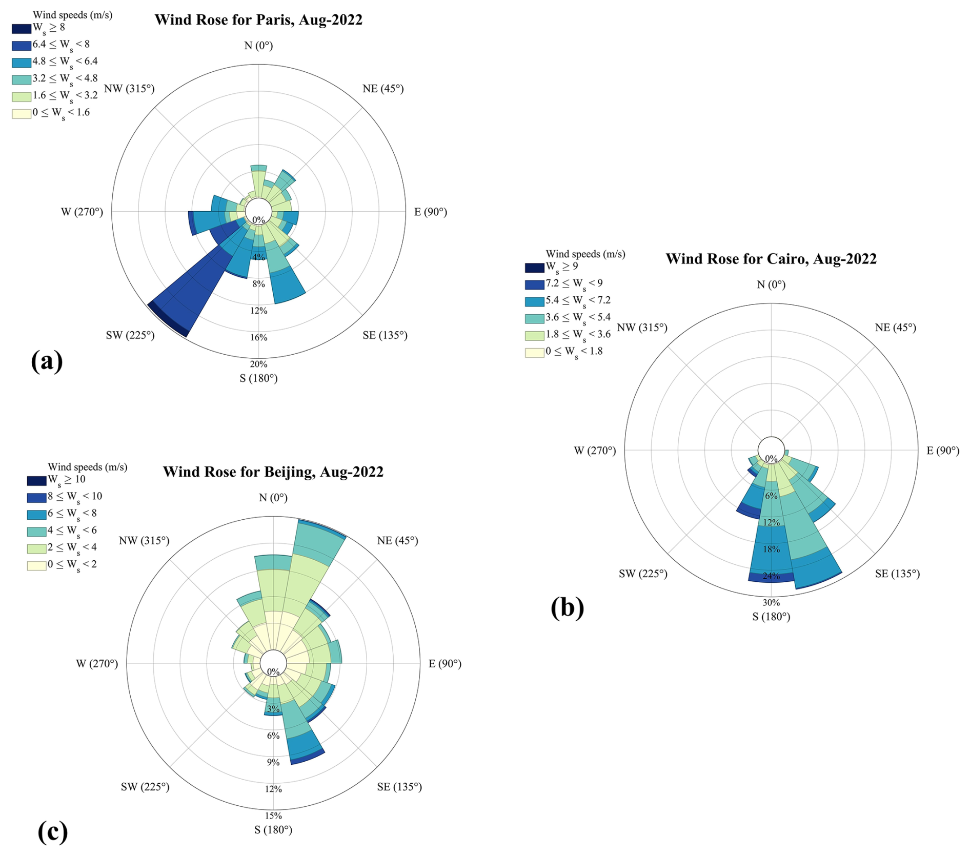
For the selected orbits, the posterior CO₂-to-NO_x ratios were 428–512 for Cairo, 731–742 for Paris, and 553–640 for Beijing (Table 2). These ratios exhibited clear temporal variability under different background conditions. The magnitude of emissions captured by each orbit depended strongly on its distance from major emission regions and the contemporaneous domain-averaged wind conditions (Che et al., 2022). The domain-averaged wind speeds for the study month (Fig. 9), as well as the high-resolution wind fields at overpass time (black arrows in Figs. 5–7), were consistently greater than 3 m s⁻¹. Under such meteorological conditions, the posterior estimates represent emissions from several hours prior to satellite overpass. The posterior uncertainties of the CO₂-to-NO_x ratio were 15.09 %–18.86 % for Cairo, 14.72 %–18.67 % for Paris, and 14.08 %–16.24 % for Beijing. Overall, uncertainties were larger for Cairo and Paris compared with Beijing.

Figure 9 Monthly mean wind rose plots for Cairo, Paris, and Beijing in August.

As described in Sect. 4.1, the prior uncertainty of the CO₂-to-NO_x ratio was prescribed based on available statistics and emission characteristics. Owing to more comprehensive statistics and advanced manufacturing processes, large metropolitan areas typically exhibit better-characterized emission features. Accordingly, the prior uncertainties for Beijing and Paris were smaller than those for Cairo. Table 2 further shows that the relative contributions of observational and transport errors differed across cities. In Cairo, transport errors dominated over observational errors, whereas in Paris the opposite held true. For Beijing, the relative magnitudes of transport and observational errors varied across orbits. The overall smaller posterior uncertainty for Beijing compared to Cairo and Paris reflects its more stable prior emission characteristics.

3.3 The Uncertainty of Transport Model

Atmospheric transport modeling uncertainty has been recognized as a major factor affecting emission constraints (Wu et al., 2018). Systematic errors arising from a combination of transport model biases and misrepresented statistical inputs can reduce the magnitude and spatial coverage of terrestrial uncertainty reductions by roughly a factor of two. Notably, transport-related uncertainties in ffXCO₂ represent a key source of error in inverse emission estimates (Ye et al., 2020). In this section, we quantify the impact of transport errors on simulated XCO₂ arising from uncertainties in horizontal wind fields and vertical mixing, with a focus on their influence on the inversion of ffXCO₂ fluxes.

Errors induced by wind field uncertainties propagate through the model and affect the accuracy of CO₂ emission estimates (Sheng et al., 2025). Previous studies have accounted for column transport errors by weighting variance relative to pressure and treating each model level independently (Lin and Gerbig, 2005; Wu et al., 2018). Ye et al. (2020) further quantified ffXCO₂ simulation uncertainty by introducing random perturbations in wind speed and direction (Ye et al., 2020). Building on these approaches, we investigate how horizontal wind speed and wind direction errors influence inversion performance.

Here, horizontal transport error is propagated through the model via its effect on ffXCO₂ plume dispersion (Luo et al., 2026; Qu et al., 2026). For the selected cities, errors are assumed to be unbiased. Wind direction uncertainty is represented by rotating the plume around the emission center, followed by the addition of random wind speed perturbations to the rotated plume. Using DQ-1 wind field data, random errors were added at each model level (wind direction perturbation between −10° and 10°, wind speed perturbation between −1 and 1 m s⁻¹), and the STILT footprints were recomputed to obtain plume-averaged footprints with random errors included (Yi et al., 2025a).

In total, 10⁴ simulations were conducted, with the ffXCO₂ integrated along each satellite track. The standard deviation (1σ) of these simulations is used to represent the uncertainty in simulated ffXCO₂ resulting from horizontal transport errors (Fig. 10).

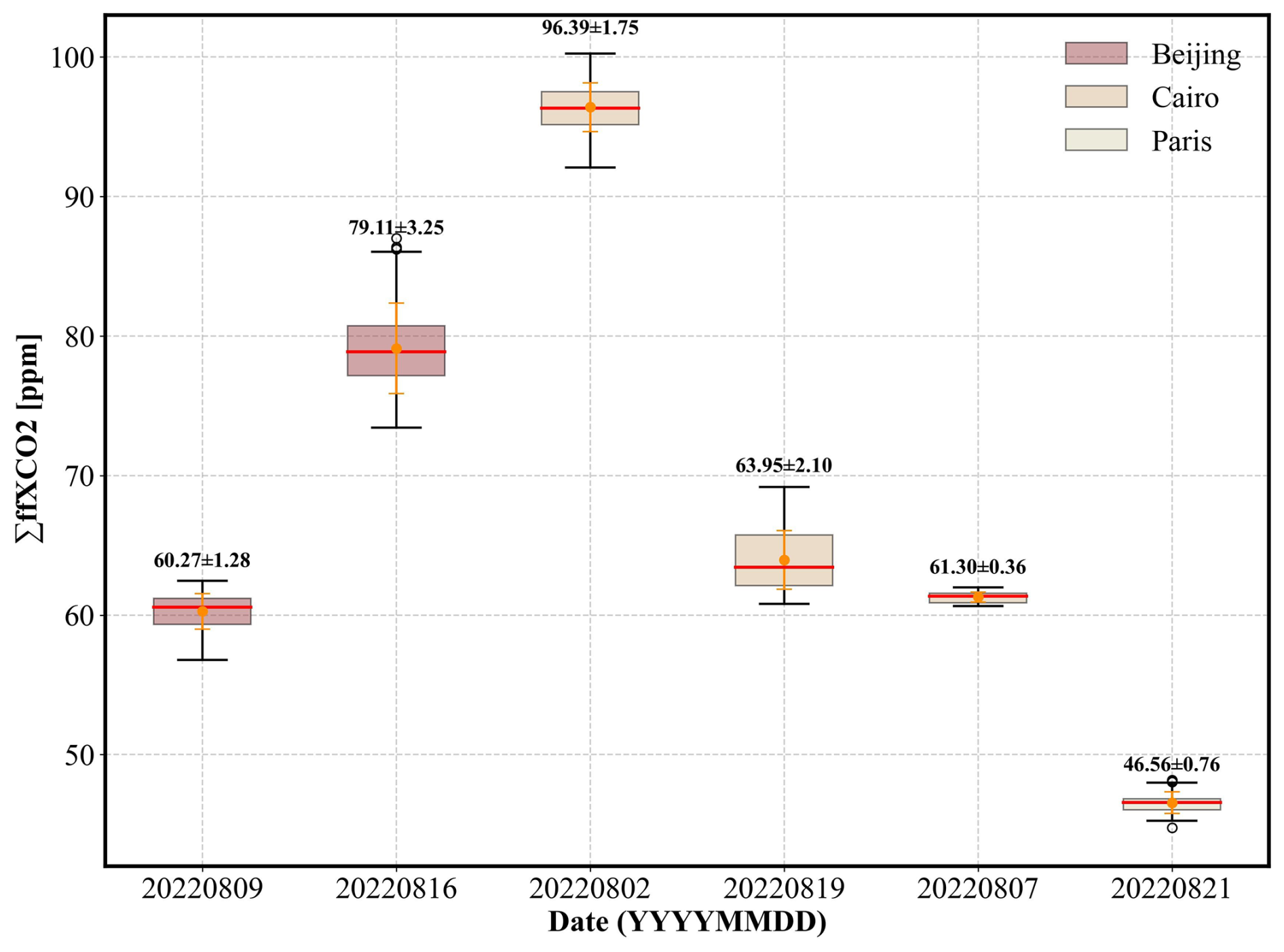
Figure 10 Boxplots of modeled integrated ffXCO₂ enhancements ffXCO₂ along selected DQ-1 overpasses for the three cities (distinguished by box color) with dates labeled on the x-axis. For each box, the central line represents the median (q2), and the bottom and top edges represent the 25th and 75th percentiles (q1 and q3), respectively. Whiskers extend to the minimum and maximum values. Numbers indicate the mean ± standard deviation.

Figure 10 presents the total simulated ffXCO₂ along DQ-1 overpasses for the different study regions. Overall, the simulated ffXCO₂ totals for the three cities are of comparable magnitude. Notably, compared with Beijing and Cairo, the horizontal transport uncertainty along the two Parisian tracks is the lowest, at 0.36 and 0.76 ppm, respectively. In Cairo, the satellite tracks traverse the edges of emission plumes, making the simulations highly sensitive to wind speed and direction, which results in larger transport model errors. Beijing, with its complex terrain and variable wind fields, exhibits more intricate transport uncertainties relative to the other two cities. These observations indicate that transport model uncertainty is closely related to city-scale emissions, the relative alignment of plumes and satellite tracks, model performance, and local topography. Variations in these factors contribute to temporal changes in posterior emission uncertainties along different tracks.

Vertical turbulent mixing governs the vertical transport of air parcels and controls the dilution of surface emissions within the boundary layer (Vertical mixing in atmospheric tracer transport models: error characterization and propagation). Although column-integrated measurements may be less sensitive to the vertical distribution of tracers than in situ observations, errors in planetary boundary layer (PBL) height can still affect column simulations due to wind shear and its interaction with vertical redistribution of tracers (Planetary boundary layer errors in mesoscale inversions of column-integrated CO₂ measurements). It is worth noting that the ACDL instrument includes an aerosol channel capable of providing extinction coefficient profiles and planetary boundary layer height (PBLH) products (Dai et al., 2024). In this study, PBLH data derived from ACDL retrievals are used in the simulations, helping to mitigate errors arising from inaccurate boundary layer height assumptions. Therefore, boundary layer height errors are not considered in the estimation of ffXCO₂.

4 Importance of Satellite Observations for Optimizing the CO₂-to-NO_x Ratio

4.1 Variations in CO₂-to-NO_x ratio calculation methods

We systematically accounted for the uncertainties associated with the prior CO₂-to-NO_x ratios for each method (see Sect. 2.2.1 (4) M1–M6). The uncertainty of the CO₂-to-NO_x ratio arises from the uncertainties of the underlying emissions. For Method 1, a Monte Carlo simulation was performed: CO₂ and NO_x inventory uncertainties (Wang et al., 2013) were used to generate random perturbations at each grid, and the CO₂-to-NO_x ratio was recalculated 10 000 times to obtain the distribution characteristics. The prior CO₂-to-NO_x ratio uncertainty was expressed as R90/M, where R90 is the range between the 95th and 5th percentiles and M is the median value from 10 000 Monte Carlo simulations. For Method 2, the uncertainty was represented as:

$$\begin{array}{}\text{(14)}& {\mathit{\sigma }}_{\mathrm{C}/\mathrm{N}}=\sqrt[\mathrm{2}]{{\mathit{\sigma }}_{{\mathrm{NO}}_x}^{\mathrm{2}}+{\mathit{\sigma }}_{{\mathrm{ffCO}}_{\mathrm{2}}}^{\mathrm{2}}}\end{array}$$

where ${\mathit{\sigma }}_{{\mathrm{NO}}_x}$ and ${\mathit{\sigma }}_{{\mathrm{ffCO}}_{\mathrm{2}}}$ denote the uncertainties of the NO_x and ffCO₂ emission factors, respectively. Notably, for each method, the use of different inventories requires adjustment of the assigned uncertainties (see Appendix A6). In Method 3, the prior CO₂-to-NO_x ratio uncertainty was derived from the quadratic sum of observational uncertainties in NO₂ and CO₂ concentrations and the Gaussian fitting uncertainty.

In this section, we used six different CO₂-to-NO_x ratio calculation methods to estimate the city-scale ratios for Beijing, Cairo, and Paris in August. Since the MEIC inventory is only available for Beijing, six prior CO₂-to-NO_x ratios were obtained for Beijing, while five ratios were derived for Paris and Cairo. Figure 11 presents the CO₂-to-NO_x ratios and their associated uncertainties for each city using the different methods. We also calculated the mean and standard deviation of the ratios across methods for each city, reflecting both the overall understanding of the city-scale prior CO₂-to-NO_x ratio and the variability arising from methodological differences.

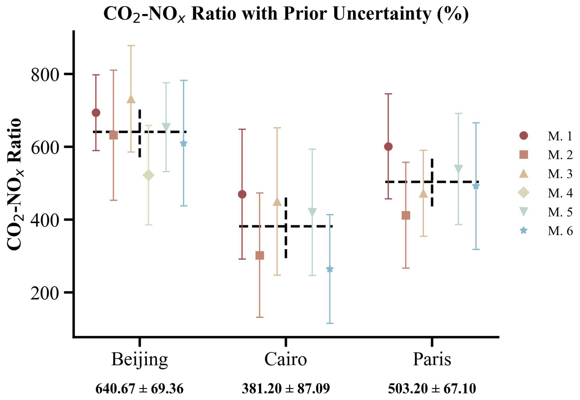
Figure 11 Results of CO₂-to-NO_x ratios obtained using different calculation methods for Beijing, Cairo, and Paris. Different CO₂-to-NO_x ratios within the same city are distinguished by color. Additionally, the mean and standard deviation of the different ratios for each city are also shown.

The results consistently show the ordering Beijing > Paris > Cairo. Moreover, more developed cities typically have better production technologies and more detailed emission statistics (Oda et al., 2019; Ye et al., 2020). Consequently, the prior uncertainties for Beijing and Paris are notably smaller than those for Cairo, and the variability of CO₂-to-NO_x ratios across methods is also reduced for these cities.

4.2 Bayesian Inversion for Reducing CO₂-to-NO_x Ratio Uncertainty

Using different prior CO₂-to-NO_x ratios, we conducted the Bayesian inversion described in Sect. 2.2.2 to optimize the August CO₂-to-NO_x ratios for Beijing, Cairo, and Paris along the respective DQ-1 satellite overpasses. Figure 12 shows the absolute reduction in posterior uncertainty (posterior minus prior) and the relative reduction (prior minus posterior, divided by prior) for each city across different orbits. For Beijing, the posterior uncertainty decreased by 9.75 %–20.88 %, corresponding to a 31.4 %–56.49 % reduction relative to the prior. In Cairo, the posterior uncertainty decreased by 21.74 %–38.87 %, equivalent to a 51.8 %–66.63 % reduction, while in Paris the reduction ranged from 11.24 %–20.09 %, corresponding to a 34.22 %–51.13 % decrease relative to the prior.

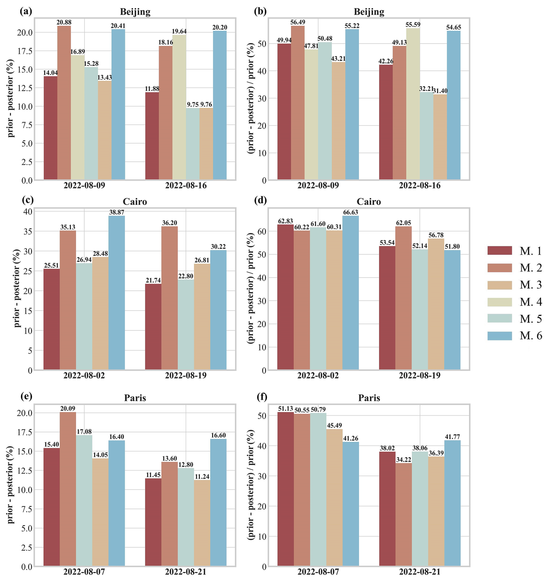
Figure 12 Comparison of Bayesian inversion prior and posterior uncertainties for each orbit over different cities. Panels (a), (c), (e) show the absolute reduction in uncertainty (prior uncertainty minus posterior uncertainty), while panels (b), (d, (f) show the relative reduction in uncertainty (prior minus posterior uncertainty divided by prior uncertainty). Results from different prior CO₂-to-NO_x ratios are represented by bars in different colors, with the values displayed at the top of each bar.

These results indicate that, for all cities, the posterior uncertainties were significantly reduced regardless of the method used to calculate the prior ratio. This demonstrates that constraining the inversion with DQ-1 ACDL observations substantially improves the accuracy of ffCO₂ estimates derived from NO_x emissions. Notably, in Cairo – the city with the largest prior uncertainty – the reduction in uncertainty after constraining with both active and passive satellite observations was the greatest, highlighting the effectiveness of satellite data in mitigating emission uncertainties in cities with incomplete statistical information. These findings underscore the potential of satellite remote sensing to supplement emission inventories and enhance the reliability of urban emission estimates.

Furthermore, we examined the range of CO₂-to-NO_x ratios calculated for each city using different methods (Fig. 13). In the figure, the black boxes represent the prior distribution ranges, while the red boxes indicate the posterior distribution ranges. The distribution ranges illustrate the variability among CO₂-to-NO_x ratios obtained from different methods, and we also quantified the reduction of the posterior range relative to the prior. Except for the orbit over Paris on 21 August, all other results show that the posterior ranges were reduced by more than 60 % compared to the priors.

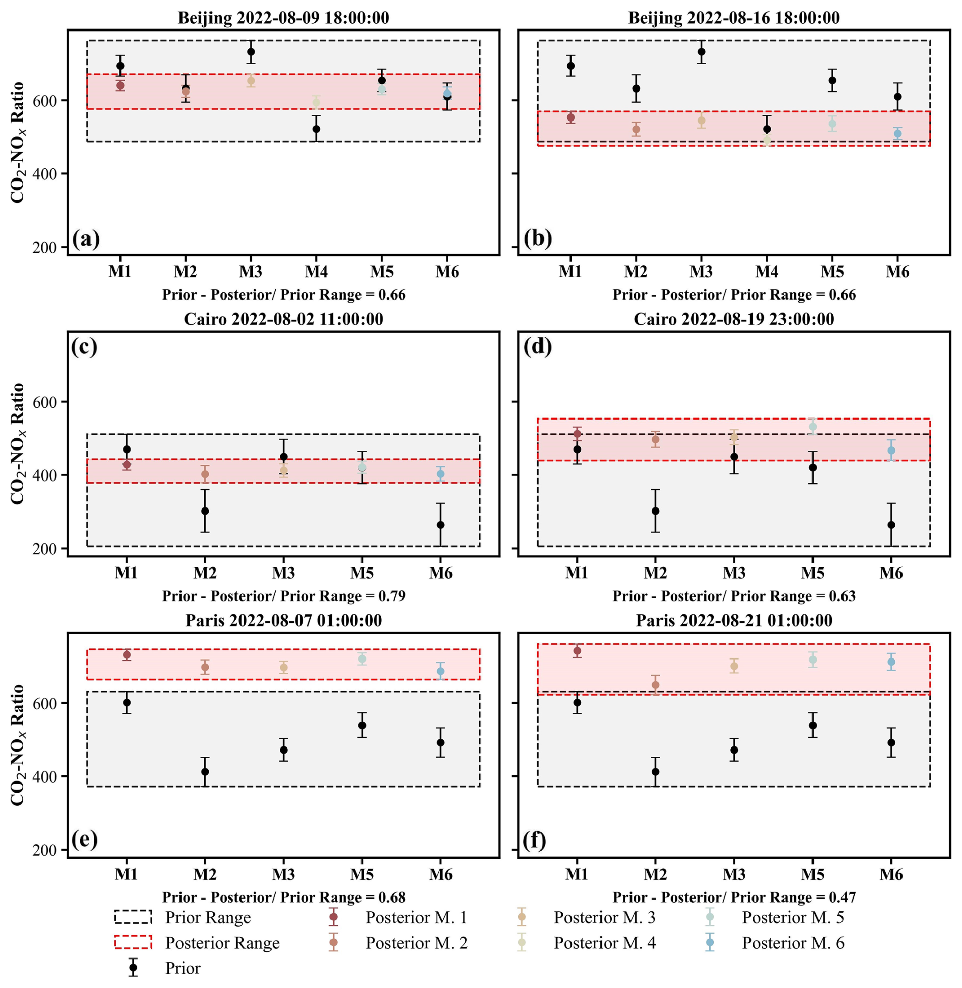
Figure 13 Distribution ranges of prior and posterior CO₂-to-NO_x ratios calculated using different methods. Black boxes represent the range of prior CO₂-to-NO_x ratios, with posterior ratios indicated by black circles. Red boxes represent the range of posterior CO₂-to-NO_x ratios, with posterior uncertainties from different methods shown using different colors and symbols.

These results demonstrate that our approach effectively reduces the discrepancies arising from different CO₂-to-NO_x ratio calculation methods. That is, prior ratios derived from various methods are constrained to approximately the same range after inversion. This finding underscores the importance of using observational constraints to obtain more accurate CO₂-to-NO_x ratios in future ffCO₂ emission estimations.

5 Summary

Accurate identification and quantification of anthropogenic CO₂ emissions form a critical scientific basis for national emission reduction policies and carbon sink strategies. However, bottom-up inventory approaches typically operate on long compilation cycles (e.g., annual), making it difficult to capture short-term or near-real-time emission dynamics. Most inventories provide only annual totals and lack the temporal resolution needed to characterize daily, hourly, or event-driven emissions.

In this study, we developed a city-scale ffCO₂ inversion framework that integrates both active and passive satellite observations of greenhouse gases. This framework enables high-resolution estimation of fossil fuel emissions at satellite overpass times and over preceding hours, while simultaneously constraining the city-scale CO₂-to-NO_x ratio. A key feature of the approach is its reduced reliance on prior emission inventories, allowing rapid and objective identification and quantification of anthropogenic emission signals at regional scales, thereby enhancing the monitoring and verification of urban emission dynamics. In this framework, satellite-observed XCO₂ enhancements attributed to urban emissions are used to constrain WRF-STILT atmospheric transport simulations of anthropogenic CO₂. This process not only enables quantitative assessment of urban fossil fuel emissions but also provides independent evidence for improving emission inventories and refining urban carbon accounting systems. The study highlights the potential of combining multi-source satellite observations with transport models and lays a foundation for future city-scale ffCO₂ inversions based on the CO₂-to-NO_x ratio. Furthermore, we discuss the impact of the lack of standardized CO₂-to-NO_x ratio calculation methods on urban emission estimates and demonstrate that observational constraints on city-scale ratios can substantially improve ffCO₂ estimation from a carbon-nitrogen co-optimization perspective. Using a Bayesian inversion approach, we optimized the CO₂-to-NO_x ratios for Cairo, Paris, and Beijing in August 2022 based on DQ-1 satellite overpasses and estimated the cities' fossil fuel CO₂ emissions using TROPOMI NO₂ data. The resulting CO₂-to-NO_x ratios ranged from 428–512, 731–742, and 553–640 for Cairo, Paris, and Beijing, respectively, indicating significant day-to-day variability in emission estimates. Cairo exhibited the largest posterior uncertainty, primarily due to high prior uncertainty and transport model errors. Differences in posterior uncertainties across orbits were also closely related to meteorological conditions and the relative position of the satellite tracks to urban plumes. We further compared ffXCO₂ enhancement distributions simulated using the ODIAC inventory. Results for Cairo and Paris were broadly consistent with TROPOMI-based simulations, while notable differences emerged for Beijing. TCCON XCO₂ observations were used to interpret these discrepancies. The monthly mean ffXCO₂ enhancement derived from TROPOMI NO₂ data differed from TCCON measurements by less than 1 ppm, whereas the ODIAC-based results deviated by 5.16 ppm. This highlights the need to account for uncertainties arising from inventory allocation and outdated updates when interpreting XCO₂ inversion results. We systematically examined the impact of different prior CO₂-to-NO_x ratio calculation methods on urban ffCO₂ inversions. In our study, methodological differences led to variations of 10.8 %–22.8 % in prior ratios. Importantly, regardless of the prior ratio or its uncertainty, DQ-1 observations constrained the posterior values to a similar range, substantially reducing discrepancies among different calculation methods. Another limitation concerns the uncertainty of the divergence-derived NO_x emissions. Although monthly averaging reduces random noise, it does not guarantee that daily divergence errors average to zero. Sampling biases related to clouds, aerosols, surface reflectance, and photochemical variability may persist in the monthly mean. Moreover, gradient operations can amplify white noise in the NO₂ column field and generate structured artifacts in the derived fluxes. Therefore, the current uncertainty estimates should be interpreted as lower-bound, first-order uncertainty estimates. Future work should include more explicit noise-filtering and detection-limit analyses, ideally using ensemble perturbations of the original Level-2 NO₂ observations and high-resolution chemical transport simulations to better represent NO₂ profile shapes, lifetimes, and NO_x:NO₂ conversion factors (Cifuentes et al., 2025; Guan et al., 2026; Wang et al., 2025; Zhang et al., 2026)

Looking ahead, improving satellite-based city-scale ffCO₂ inversions will require accounting for the spatiotemporal correlations of prior emission errors. Our current framework does not yet incorporate this aspect, which imposes certain limitations on the interpretation and application of the results. Satellite observations are inherently constrained by inversion errors, sampling geometry, and revisit frequency, limiting overpass opportunities. A single prior factor, such as a uniform CO₂-to-NO_x ratio, cannot fully capture the complex spatiotemporal features of emissions. Incorporating prior error correlations can mitigate uncertainties arising from sparse observations and better resolve temporal and spatial variability in urban emissions. Moreover, the number of satellite tracks required to constrain city emissions depends on the desired emission resolution and uncertainty thresholds relevant for policy applications. Lower temporal resolution may suffice for long-term trend analysis, whereas capturing short-term peaks or episodic emissions necessitates higher observation frequency and precision. This consideration aligns with emerging international approaches emphasizing multi-platform, multi-temporal observations, combining polar-orbiting, geostationary satellites, and ground-based monitoring to achieve multidimensional constraints on urban emissions.

Overall, our results demonstrate that coupling high-resolution atmospheric transport simulations with a Bayesian inversion framework allows TROPOMI and DQ-1 multi-source observations to effectively constrain urban ffXCO₂ enhancement signals. The approach captures spatial heterogeneity of emissions, particularly in cities with strong emission intensities and well-defined plume structures, providing a robust basis for quantitative analysis. Furthermore, current methods estimating ffCO₂ from NO_x emissions often lack explicit treatment of CO₂-to-NO_x ratio uncertainty, which can significantly influence inversion outcomes. Differences among calculation methods for the same region can be as large as 258–304. Notably, our inversion framework substantially reduces CO₂-to-NO_x ratio uncertainty, providing more stable priors for urban ffCO₂ estimation. Recent studies suggest the need to further optimize CO₂-to-NO_x emission ratios at regional scales to improve ffCO₂ estimates (Feng et al., 2024). Therefore, we recommend that future NO_x-based ffCO₂ inversion studies adopt observational constraints to refine CO₂-to-NO_x ratios, minimizing errors arising from prior ratio uncertainties.

Appendix A

A1 ACDL XCO₂ Data Inversion

Unlike passive satellite XCO₂ products (e.g., OCO-2/3), the DQ-1 XCO₂ product – hereafter referred to as ${X{\mathrm{CO}}_{\mathrm{2}}}^{\text{Lidar}}$ to distinguish it from passive measurements – is derived from the differential absorption between ACDL's on-band wavelength (strong CO₂ absorption) and off-band wavelength (weak CO₂ absorption). Here, “WF(p)” refers to the lidar signal and integrated weighting function introduced in Sect. 2.1.1, with “p” representing atmospheric pressure:

$$\begin{array}{}\text{(A1)}& {X{\mathrm{CO}}_{\mathrm{2}}}^{\text{Lidar}}={\displaystyle \frac{\mathrm{2}\times \ln \left(\frac{V_{\text{off}}\times V_{\text{on}-\mathrm{0}}}{V_{\text{on}}\times V_{\text{off}-\mathrm{0}}}\right)}{{\int }_{\text{p\_surface}}^{\text{p\_toa}}\text{WF(p)}\mathrm{d}p}}\end{array}$$

here, V_on and V_off denote the reflected signal energies at the on-band and off-band wavelengths, respectively, while V_on−0 and V_off−0 correspond to the transmitted signal energies. p_surface represents the atmospheric pressure at the sub-satellite point of the laser, and p_toa denotes the pressure at the top of the atmosphere. The denominator in Eq. (A1) represents the integrated weighting function (WF(p)), which can be expressed according to Refaat et al. (2016) as:

$$\begin{array}{}\text{(A2)}& \text{WF(p)}=\mathrm{\Delta }{\mathit{\sigma }}_{\text{wf}}({\mathit{\lambda }}_{\text{on}},{\mathit{\lambda }}_{\text{off}},p)\times N_{\text{dry}}\left(p\right)\end{array}$$

here, $\mathrm{\Delta }{\mathit{\sigma }}_{\text{wf}}({\mathit{\lambda }}_{\text{on}},{\mathit{\lambda }}_{\text{off}},p)$ represents the differential absorption cross-section of CO₂ between the on-band λ_on and off-band λ_off wavelengths at pressure p. N_dry denotes the number of dry air molecules per unit area within the corresponding pressure layer.

Table A1 DQ-1 ACDL operating parameters.

A2 Derivation of the Principle of Mass Balance

For satellite column observations of specific species such as NO₂, the mass balance equation can be expressed as follows:

$$\begin{array}{}\text{(A3)}& \left\{\begin{array}{l}\frac{\partial V_{{\mathrm{NO}}_{\mathrm{2}}}}{\partial t}+\mathrm{\nabla }\times {\mathit{F}}_{{\mathrm{NO}}_{\mathrm{2}}}=E_{{\mathrm{NO}}_{\mathrm{2}}}-S\\ {\mathit{F}}_{{\mathrm{NO}}_{\mathrm{2}}}=V_{{\mathrm{NO}}_{\mathrm{2}}}{\mathit{u}}_{\mathrm{100}}\\ S\approx \frac{V_{{\mathrm{NO}}_{\mathrm{2}}}}{\mathit{\tau }}\end{array}\right.\end{array}$$

here, $V_{{\mathrm{NO}}_{\mathrm{2}}}$ represents the columnar NO₂ concentration observed by TROPOMI, defined as a scalar function of x and $\mathrm{\nabla }=(\partial /\partial x,\partial /\partial y)$ denotes the gradient operator; $={\mathit{F}}_{{\mathrm{NO}}_{\mathrm{2}}}(F_x,F_y{)}^{\mathrm{T}}$ is the horizontal flux, with units of $\mathrm{mol}{\mathrm{m}}^{-\mathrm{2}}{\mathrm{s}}^{-\mathrm{1}}$, expressed as a vector function of x and y and weighted by the wind vector. The 100 m wind field is commonly used to characterize horizontal transport within the planetary boundary layer (PBL, Sun, 2022). τ represents the first-order chemical lifetime of NO₂ in seconds.

By solving the system of equations in Eq. (A3) and expanding the horizontal flux divergence using vector calculus, we obtain the derivation of Eq. (A4) from Eq. (A3):

$$\begin{array}{}\text{(A4)}& \left\{\begin{array}{l}{\mathit{u}}_{\mathrm{100}}\times \left(\mathrm{\nabla }{V}_{\mathrm{NO}}\right)+V_{\mathrm{NO}}(\mathrm{\nabla }\times {\mathit{u}}_{\mathrm{100}})=\mathrm{\nabla }\times {\mathit{F}}_{{\mathrm{NO}}_{\mathrm{2}}}\\ E_{{\mathrm{NO}}_{\mathrm{2}}}=\frac{\partial V_{{\mathrm{NO}}_{\mathrm{2}}}}{\partial t}+\mathrm{\nabla }\times {\mathit{F}}_{{\mathrm{NO}}_{\mathrm{2}}}+\frac{V_{\mathrm{NO}}}{\mathit{\tau }}\end{array}\right.\end{array}$$

Sun (2022), in their first-principles derivation, introduced a “topographic correction term” to replace the wind divergence term V_NO(∇×u₁₀₀). Beirle et al. (2023) demonstrated that incorporating a topographic correction significantly improves the inversion of power-plant NO_x emissions based on the divergence method. Koene et al. (2024) carefully compared these two terms in the derivation of the divergence method, showing that they originate from the continuity equations of the source and non-source terms, and that numerically, the wind divergence and wind–topography terms are approximately equal in the absence of observational errors.

Despite their numerical equivalence in derivation, the accuracy of reanalyzed wind fields is generally lower than that of surface elevation data. Therefore, in practical measurements – particularly in complex, fine-scale settings – the wind divergence term alone may not provide sufficient constraint. Correcting wind divergence artifacts using topographic gradients is more feasible, especially in regions with rugged terrain. Accordingly, we revise Eq. (A5) using Eq. (A4) as follows:

$$\begin{array}{}\text{(A5)}& {\displaystyle \frac{V_{{\mathrm{NO}}_{\mathrm{2}}}{\mathit{u}}_{\mathrm{10}}\times \left(\mathrm{\nabla }{z}_{\mathrm{0}}\right)}{H}}\approx V_{{\mathrm{NO}}_{\mathrm{2}}}(\mathrm{\nabla }\times {\mathit{u}}_{\mathrm{100}})\end{array}$$

here, $\frac{V_{{\mathrm{NO}}_{\mathrm{2}}}{\mathit{u}}_{\mathrm{10}}\times \left(\mathrm{\nabla }{z}_{\mathrm{0}}\right)}{H}$ represents the topographic correction term, where the 10 m wind is approximated as the near-surface wind, and H denotes the gas scale height in meters. Following previous studies (Beirle et al., 2023; Sun, 2022; Liu et al., 2021), Eq. (A5) is assimilated over both temporal and spatial dimensions. This procedure is concisely represented using the operator 〈f〉, as introduced in the derivations by Liu et al. and Sun et al. Ultimately, this approach allows the derivation of the vertical NO₂ flux on a grid-resolved basis.

A3 Atmospheric Model Setting

In this study's application of STILT, hourly outputs from version 4.0 of WRF are used to provide high resolution meteorological fields, with the model grid configured to 32 vertical (eta) layers. The 6 hourly NCEP FNL (Final) global operational analysis data (ds083.3, 0.25°×0.25°) are used as initial and boundary conditions for meteorological and land surface fields to provide the initial and boundary conditions for WRF runs. The simulations run for 30 h, but only the 7th to 30th hours of each simulation are used to avoid spin-up effects in the first 6 h.

In this study, we used the STILT model, version 2, to simulate atmospheric transport processes. STILT is configured to release 500 particles per receptor each time, with forward dispersion over 24 h. The particle release heights for STILT are set within the range of 50–1000 m, with releases every 50 m, and 1000–2000 m, with releases every 100 m, the spatial resolution of the STILT simulations is 1 km×1 km. Generally, as MAXAGL increases from 1–2 km, the urban enhancement increases and then stabilizes.

Table A2 Model version information used in this study.

A4 Calculation of NEE XCO₂ enhancement

We performed vertical integration following the method provided by the TCCON team, using the 51 altitude levels listed in the publicly available ak_altitude dataset, which also serve as input heights for the STILT model. In contrast to the XSTILT calculation method used for DQ-1, we applied the integration operator integration_operator_x2019 together with the mean averaging kernel ak_xco2 to the STILT footprints across the 51 levels in order to generate the simulated XSTILT values required for this study. We selected the National Institute for Environmental Studies (Japan) data-driven Upscale Product of Global Gross Primary Production (NEE) as the reference for the overall local NEE during the DQ-1 overpasses. By convolving the NEE inventory with XSTILT, we simulated the XCO₂ enhancement at TCCON sites attributable to NEE.

A5 Calculation of Priori NO_x Emission Uncertainty

The uncertainty estimated here should be regarded as a first-order propagated uncertainty rather than the full uncertainty of the divergence-derived NO_x emissions. In particular, this formulation does not fully capture structured errors arising from finite-difference gradient operators, oversampling from Level-2 observations to Level-3 grids, non-Gaussian retrieval noise, or sampling biases caused by clouds, aerosols, surface reflectance, and photochemical variability. The uncertainty of the NO_x inventory derived from the mass balance approach can be estimated using the error propagation law as follows:

$$\begin{array}{}\text{(A6)}& {\mathit{\epsilon }}_{{\mathrm{NO}}_x}=\sqrt[\mathrm{2}]{{\mathit{\epsilon }}_{\mathit{\alpha }}^{\mathrm{2}}+{\mathit{\epsilon }}_{\mathrm{NO}}^{\mathrm{2}}}\end{array}$$

where ε_α represents the uncertainty in the NO_x$/$NO₂ ratio, its uncertainty arises from the uncertainties in the input parameters of the chemical model (Liu et al., 2022). And ${\mathit{\epsilon }}_{{\mathrm{NO}}_{\mathrm{2}}}$ denotes the uncertainty in the NO₂ flux field. The latter can be further decomposed as:

$$\begin{array}{}\text{(A7)}& {\mathit{\epsilon }}_{\mathrm{NO}}=\sqrt[\mathrm{2}]{{\mathit{\epsilon }}_{\text{TROPOMI}}^{\mathrm{2}}+{\mathit{\epsilon }}_{\text{Wind}}^{\mathrm{2}}+{\mathit{\epsilon }}_{\text{Fit}}^{\mathrm{2}}}\end{array}$$

here, ε_TROPOMI is the uncertainty of the NO₂ column concentration, ε_Wind represents the uncertainty associated with the wind field, and ε_Fit accounts for the uncertainty in the fitted vertical scale height and chemical lifetime. The uncertainty of NO₂ arises from multiple factors, including spectral fitting, stratospheric correction, AMF, clouds, vertical profiles, and surface albedo (Boersma et al., 2018; Verhoelst et al., 2021; Van Geffen et al., 2022; Lu et al., 2025). In this study, we use the ratio of the standard deviation to the mean of the column concentration within the study area as a proxy for the TROPOMI observational noise, integrated over the time series. It should be noted that this proxy is calculated based on the oversampled gridded data (also referred to as Level-3) rather than the original Level-2 orbit data. In this study, we do not account for errors introduced during the oversampling of TROPOMI L2 data to the grid (Glissenaar et al., 2025). With appropriate gridding, the uncertainty in polluted areas can be reduced by approximately 20 % compared with the original orbits (Sun et al., 2018a). Wind field uncertainty is quantified through 104 Monte Carlo perturbations of wind speed and direction, with the propagated standard deviation representing the flux variability. The fitting uncertainty is obtained by performing 104 Monte Carlo draws of the grids involved in the fit, generating ensembles of scale heights and chemical lifetimes, with the final fitting error defined as the root mean square of the standard deviations of these ensembles.

Using the method described above, we quantified the overall uncertainty of NO_x prior emissions for three cities, as well as the contributions from individual components, with the detailed results summarized in Table A3. It should be noted that the uncertainties reported here represent aggregated values for the entire urban area, rather than detailed uncertainties for individual grid cells.

Based on the uncertainty calculations, the total uncertainty is on the order of ∼24 % for Beijing, ∼18 % for Paris, and ∼14 % for Cairo. A closer look at the contributions of individual components reveals that NO₂ column concentrations and the wind field are the dominant sources, together accounting for more than 66.7 % of the total uncertainty. This is attributable to the nature of data-driven dispersion models, in which uncertainties in wind and concentration directly govern the overall uncertainty (Sun, 2022). The nonlinear gradient operations in dispersion models (e.g., second-order difference operators) can amplify white noise in the original concentration field, while in existing emission quantification models, wind fields are considered a major source of uncertainty due to sparse monitoring sites and model errors (Huang et al., 2025).

Among the three cities, NO₂ column inversion uncertainty is highest in Beijing. Unlike Cairo, where high surface reflectivity eases retrievals, Beijing is located in the highly polluted North China Plain with elevated AOD, which increases the difficulty of passive column inversion. In addition, Beijing's complex terrain contributes to the highest wind field uncertainty (∼17 %) among the three cities. The NO_x$/$NO₂ uncertainty is roughly similar across the three cities, consistent with previous studies using NU-WRF ($\sim \mathrm{1.4}\pm \mathrm{0.1}$). In contrast, the uncertainty associated with first-order chemical lifetime and vertical scale height is the lowest among all components (∼1 %). This is different from earlier studies (∼15 %) (Liu et al., 2022) and reflects the benefit of the data-driven fitting approach proposed by Sun et al. (2018b) (see main text). Since no new assumptions were introduced in the current study, this uncertainty arises solely from the linear fitting model.

Table A3 The overall uncertainty of NO_x emissions and the uncertainties of individual components were derived using the dispersion model.

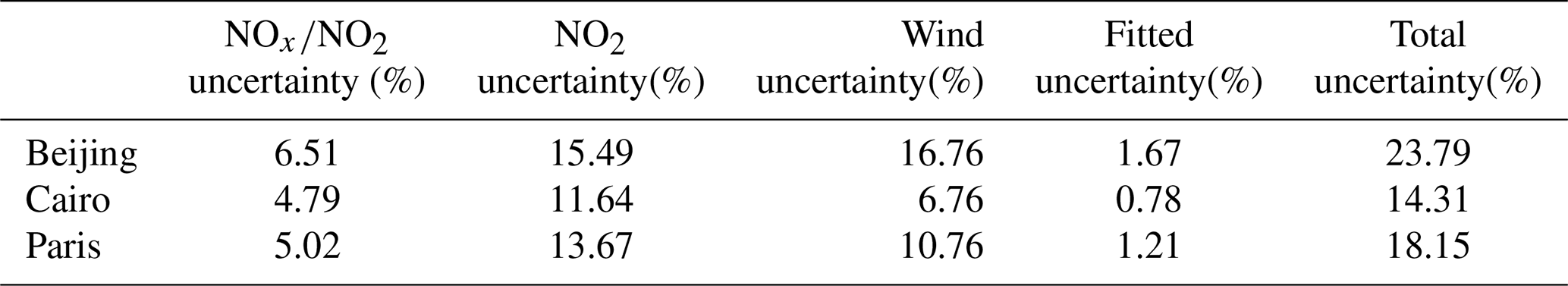
A6 Optimization results of the CO₂-to-NO_x ratio obtained using different calculation methods

Table A4 Inversion results of CO₂-to-NO_x ratios calculated using different methods.

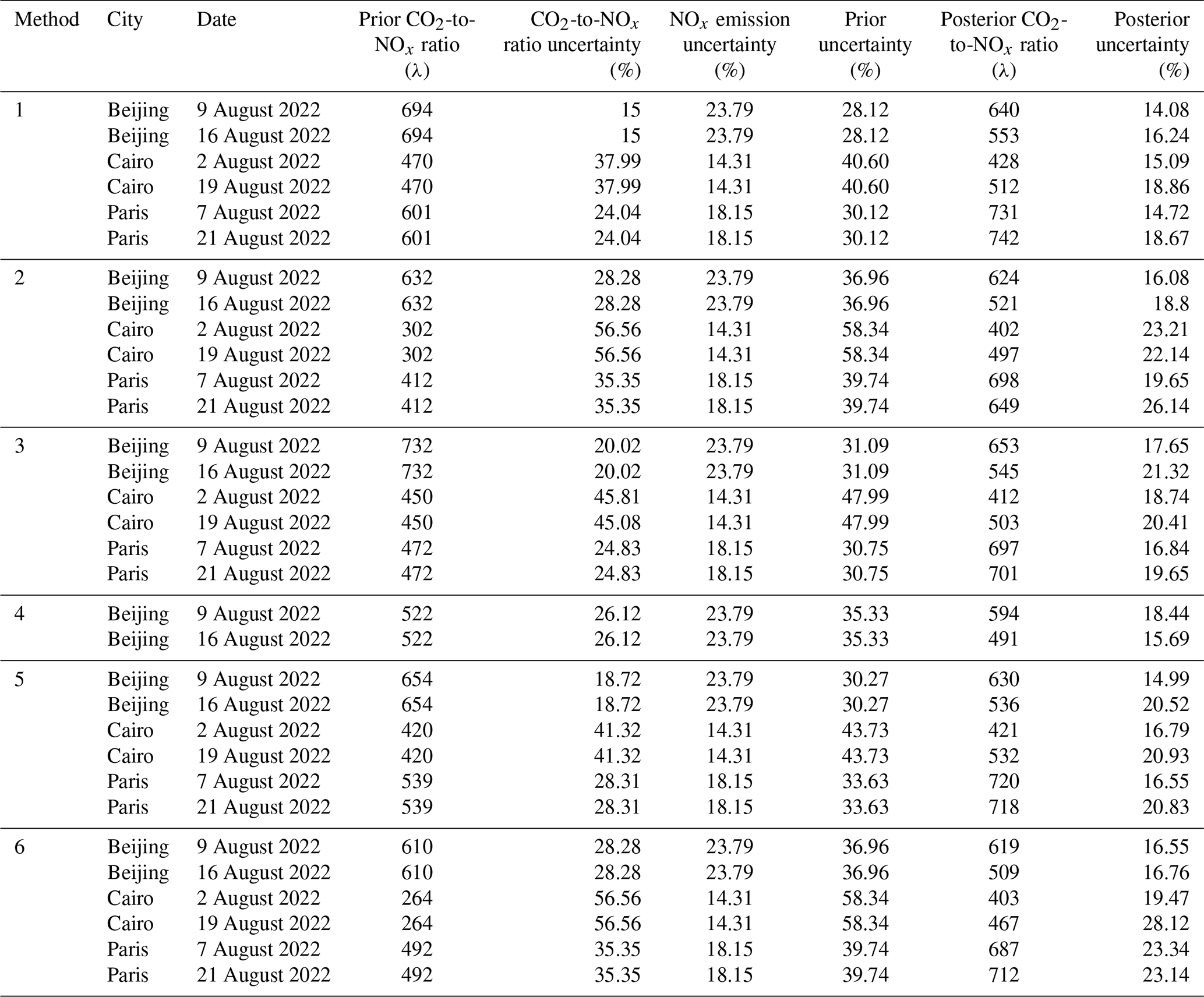
A7 Posterior fossil fuel emissions distribution for each city

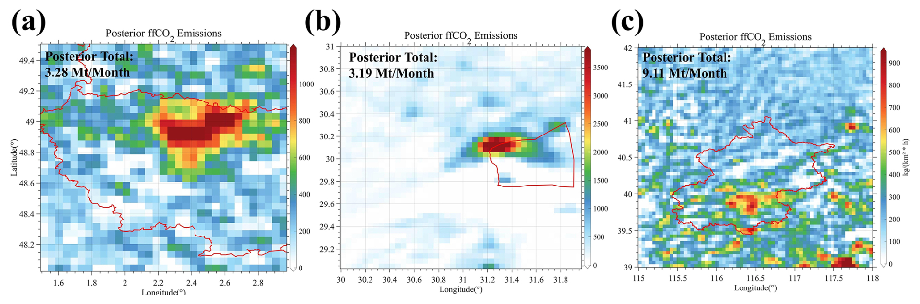
Figure A1 Posterior fossil fuel carbon dioxide emissions for each city. The red lines outline city boundaries, while the colored shading indicates carbon dioxide emission distribution.