Measurement report: Airborne observation of CO₂ and CH₄ in the urban atmospheric boundary layer in Eastern China

To characterize the concentrations of CO₂ and CH₄ in the urban atmospheric boundary layer (ABL), this study conducted airborne measurements over four cities in Eastern China, obtaining full vertical profiles (ground to 2 km) over Beijing and Nanjing, partial profiles over Hengshiu and Shangqiu. Results showed that the CO₂ and CH₄ concentrations in the ABL were consistently higher than those in the free atmosphere, with the highest values observed near the surface (Beijing and Nanjing). In Beijing, the daytime and nighttime inversion jumps in the CO₂ concentration were −25.2 ± 0.4 and −18.0 ± 0.2 ppm, respectively. In Nanjing, the corresponding values were −9.5 ± 0.1 and −10.0 ± 0.4 ppm. For CH₄, the inversion jumps were −171.4 ± 0.4 ppb during the day and −202.6 ± 2.3 ppb at night (Beijing); in Nanjing, they were −140.7 ± 0.1 and −108.0 ± 2.1 ppb, respectively. Change in the airmass trajectory altered the free-atmospheric CO₂ concentration over Nanjing by 3 ppm in a matter of a few hours. The EDGAR CH₄:CO₂ emissions ratio was within measurement uncertainty of the nighttime ABL value in Beijing, but about 80 % higher in Nanjing, indicating that the inventory may have missed the recent energy transition from gasoline and natural gas to electric in the transport sector. The experimental data is available at https://doi.org/10.7910/DVN/ZPVSVU (Wang et al., 2026).

1 Introduction

This study is an experimental investigation of atmospheric CO₂ and CH₄ in the urban atmospheric boundary layer (ABL) in Eastern China. The ABL refers to the lowest layer of air between the Earth's surface and the free atmosphere, with a typical thickness of 1 km on land. Measurements of CO₂ and CH₄ in the ABL are motivated by several scientific considerations. Observational studies of the ABL structure are usually made with potential temperature and water vapor. These two scalars are typically conserved if in the ABL when it is free of clouds and aerosols. In polluted conditions or if clouds are present, they are no longer conserved, which complicates the diagnostic analysis of the ABL depth and its time evolution (Lee, 2023). CO₂ and CH₄, on the other hand, are conserved scalars in the clear, the cloudy and the polluted ABL when chemical destruction and generation are absent. Their presence does not affect air motion. Although they may participate in chemical reactions in the ABL, these reactions have no dynamic consequence at timescales relevant to ABL processes. In regions with heavy pollution, such as Eastern China and Northern India, it is advantageous to study the ABL dynamics with CO₂ and CH₄ profiles in addition to temperature and water vapor.

CO₂ and CH₄ concentrations in the ABL reveal information on surface-air exchanges at the landscape scale (10–100 km) (e. g., Denmead et al., 1996; Xueref-Remy et al., 2011). Their vertical profiles are often used in the ABL budget framework to determine the surface fluxes. A complete budget analysis requires observation or parameterization of the ABL depth, the time rate of change of the concentration, horizontal advection, and the entrainment flux at the ABL top (Crawford et al., 2016; Vilà-Guerau de Arellano et al., 2004; Trousdell et al., 2016). In situations where horizontal advection dominates, concentration profiles observed upwind and downwind of an area source can be used in a simple box model to infer the surface flux (Hajny et al., 2019; O'Shea et al., 2014; Tomlin et al., 2023; Wratt et al., 2001). In a one-dimensional ABL without horizontal advection, the problem is simplified to the surface flux being balanced by the entrainment flux and the time rate of change of the concentration in the ABL air column (Laubach and Fritsch, 2002; Raupach et al., 1992). This column budget method, also called the slab approximation (Lee, 2023), requires that the entrainment flux be calculated as the product of the entrainment velocity and the inversion jump of concentration. While the entrainment velocity can be derived from the ABL growth rate or a parameterization equation (Vilà-Guerau de Arellano et al., 2004; Trousdell et al., 2016), the inversion jump must be measured. (The inversion jump refers to the difference in concentration across the capping inversion at the top of the ABL.) The inversion jump of CO₂ has been measured in many aircraft-based studies (Barker et al. 2021; Filges et al., 2015; Herrera et al., 2021; Laubach and Fritsch, 2002; Lloyd et al., 2001; Narbaud et al., 2023; O'Shea et al., 2014; Saito et al., 2009; Sarrat et al., 2007; Shashkov et al., 2007; Shibata et al., 2018; Xueref-Remy et al., 2011). Fewer studies have reported the CH₄ profile with large enough vertical span to include the CH₄ inversion jump (Barker et al. 2021; Filges et al., 2015; Hartery et al., 2018; Herrera et al., 2021; Narbaud et al., 2023; O'Shea et al., 2014). These CO₂ or CH₄ inversion jump observations were made over forests (Lloyd et al., 2001, Ramonet et al., 2002, Shashkov et al., 2007), grassland (Vilà-Guerau de Arellano et al., 2004), mixed land (cropland and forest; Laubach and Fritsch, 2002; Saito et al., 2009; Sarrat et al., 2007; Shibata et al., 2018), wetlands and tundra (Barker et al., 2021; Narbaud et al., 2023; O'Shea et al., 2014; Hartery et al., 2018), and a landscape dominated by animal facilities (Herrera et al., 2021). No such data exists yet for urban land.

Simultaneous measurement of multiple gases in the ABL can provide a constraint on emission intensity, emission source type and source region. Because some gases do not undergo significant chemical reactions over short timescales, the concentration ratio is widely used for source identification, for example, to distinguish between anthropogenic and natural sources or to indicate the intensity of biomass burning. Examples include C₂H₆ versus CH₄ (Joo et al., 2024), CH₄ versus CO₂ (Kenea et al., 2023; Sreenivas et al., 2016) and CO₂ versus CO (Shan et al., 2022). Additionally, it serves as a tool to verify the accuracy of emission inventories (Hajny et al., 2019; Liu et al., 2018; Shen et al., 2014). The ratio may vary with altitude due to the influence of different source and sink processes. In the ABL, the concentrations are primarily affected by local emissions (Park et al., 2022). In the free atmosphere, CO₂ and CH₄ concentration variations are influenced by transported air masses (Sreenivas et al., 2019). Here, the gas concentration ratio reflects the degree of mixing of the background air with CO₂ and CH₄ emitted regionally. When combined with back-trajectory analysis, the ratio can help infer the composition of upwind emission sources (Shan et al., 2022; Tiemoko et al., 2021). Although some studies have explored the concentration ratio at different altitudes downwind of a city and have used it to infer emission origins (Li et al., 2022; Shan et al., 2022), we are not aware of published research on the CH₄:CO₂ ratio in the ABL air column directly above urban land.

Measuring the vertical profiles of CO₂ and CH₄ concentrations in the ABL is challenging due to cost and logistical constraints. Available measurement platforms include aircraft, tethersonde, unmanned aerial vehicle (UAV), and tall tower, each having its strengths and weaknesses. Tall towers (Berhanu et al., 2016; Satar et al., 2016) and tethersondes (Crawford et al., 2016) can provide continuous monitoring, but they can only probe the lower portion of the ABL. Sensors on a tethersonde are low-cost and lightweight. Having low measurement precision, they are unable to detect small concentration variations in the ABL. Recent years have seen increasing use of UAVs (Andersen et al., 2018; Berhanu et al., 2016; Satar et al., 2016; Watai et al., 2006), but UAV operation also has payload limitation, in addition to aviation restriction on flight height (e.g., no higher than 120 m above the ground in the USA). Aircraft is the only viable option if gaseous measurements are to extend from the surface to the ABL capping inversion. Because gas analyzers on board of an airplane typically have much better precision and faster time response that those carried by a tethersonde or an UAV, aircraft observation can resolve detailed vertical structures, including the concentration jumps across the capping inversion whose thickness is on the order of 50 m. Because of high operational cost, aircraft observations are carried out in campaign mode with observational time typically less than a few hours. Even though aircraft profiles are only snapshot of conditions in the atmosphere, data of this kind makes useful contribution to the published literature. In addition to the ABL applications discussed above, they can be used for validation of ground- and space-borne sensor retrievals of atmospheric greenhouse gases (Sreenivas et al., 2019; Tanaka et al., 2012) and for evaluation of atmospheric transport models (Agustí-Panareda et al., 2023; Friedlingstein et al., 2022; Galkowski et al., 2021; Stephens et al., 2007; Tomlin et al., 2023; Vogel et al., 2023).

Regarding CO₂ and CH₄ in the urban ABL, Li et al. (2014) collected 58 profiles of CO₂ concentration up to a height of 1400 m in Xiamen City, China with a portable gas analyzer (measurement uncertainty 4 ppm) attached to a tethersonde. These profiles showed a clear diurnal pattern, although no inversion jump or a well-mixed layer was evident in the data. Another tethersonde campaign was carried out by Crawford et al. (2016) in Vancouver, Canada over a 24 h period using the same type of analyzer as in Li et al. (2014), with a profile height of 400 m. Several authors have reported the CO₂ measurement made with commercial airliners equipped with a CO₂ analyzer during their ascent and descent in several large cities in the CONTRAIL program (Umezawa et al., 2016, 2020). These profiles provide information on the advection of urban emission plumes, but they are less useful for ABL studies because of the lack of data below a height of about 800 m. In our own examination of the CONTRAIL data (Machida et al., 2018), we could not detect the ABL height or the inversion jump (due to a slow instrument response and the rapid vertical ascent or descent of the aircraft); these two features are critical for accurately estimating emissions using the ABL budget method.

The goal of this study is to characterize the vertical distributions of CO₂ and CH₄ concentrations over four urbans areas in Eastern China. They are, in order from north to south, Beijing, Hengshui, Shangqiu and Nanjing. These profile measurements were made with an analyzer on board of a research airplane that flew a round trip between Beijing and Nanjing. Detailed analysis was made of the observations in Nanjing and Beijing, which were obtained during the plane's landing and take-off and spanned the whole ABL and the lower troposphere. Specifically, we aim (1) to examine the time evolution of the profiles between landing and take-off, (2) to quantify the CO₂ and CH₄ inversion jumps (differences in concentrations across the capping inversion at the top of the ABL), and (3) to compare the CH₄:CO₂ emission ratio obtained with the concentration data with the ratio obtained with inventory data.

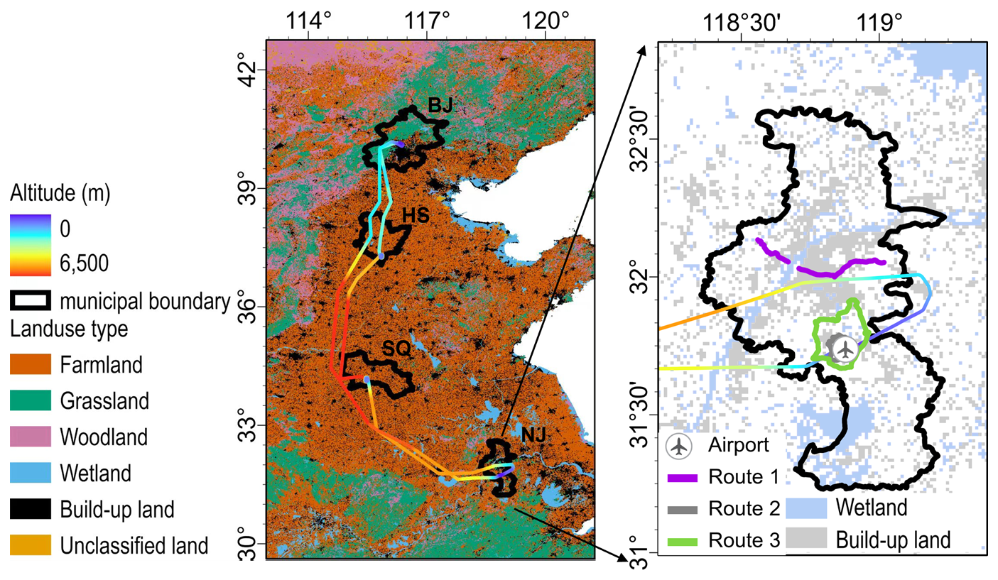
Figure 1 Left: Locations of the four cities for the vertical profile observations and flight routes; Right: takeoff and landing routes and vehicle-mounted observation routes in Nanjing. The basemap on the left shows wetland and build-up land according to Gong et al. (2019).

2 Materials and methods

2.1 Airborne observation

The airborne observation was conducted in Eastern China on 14 May 2023 (Figs. 1–3). The flight traversed Beijing, a province-level municipality, and five provinces (Hebei, Henan, Shandong, Anhui and Jiangsu). Profile measurements were made over Beijing, Hengshui, Shangqiu and Nanjing. Beijing, the capital of China, is located in the North China Plain. It has a permanent population of 21 million and covers an area of 16 000 km². The city is bordered by mountains on the west, north, and northeast sides, while the southeast is characterized by flat plains. The major GHG emission sources include industrial activities, transportation, and household energy consumption. Hengshui is situated in the southeastern part of Hebei Province, with a permanent population of 4.2 millions and a total area of 8800 km². The city comprises agricultural land and aquatic landscapes such as Hengshui Lake. GHG emissions primarily originate from industrial manufacturing, while agricultural activities also contribute CH₄ to a certain extent. Shangqiu, located in eastern Henan Province, has a permanent population of 7.7 million and spans an area of 11 000 km². Its terrain is predominantly flat. As a major grain production area and a transportation hub in China, its major emission sources include industrial production and coal mining. Nanjing, the capital of Jiangsu Province, is located in the lower reaches of Yangtze River. It has a permanent population of 9.5 million and an area of 6600 km². The urban landscape is a mix of natural and built environments. Industrial production and transportation are the primary sources of emissions in the city.

Figure 2 Flight altitude as a function of latitude. BJ: Beijing; NJ: Nanjing.

Figure 3 Photograph of the airplane (left) and the sampling inlet on the airplane (right).

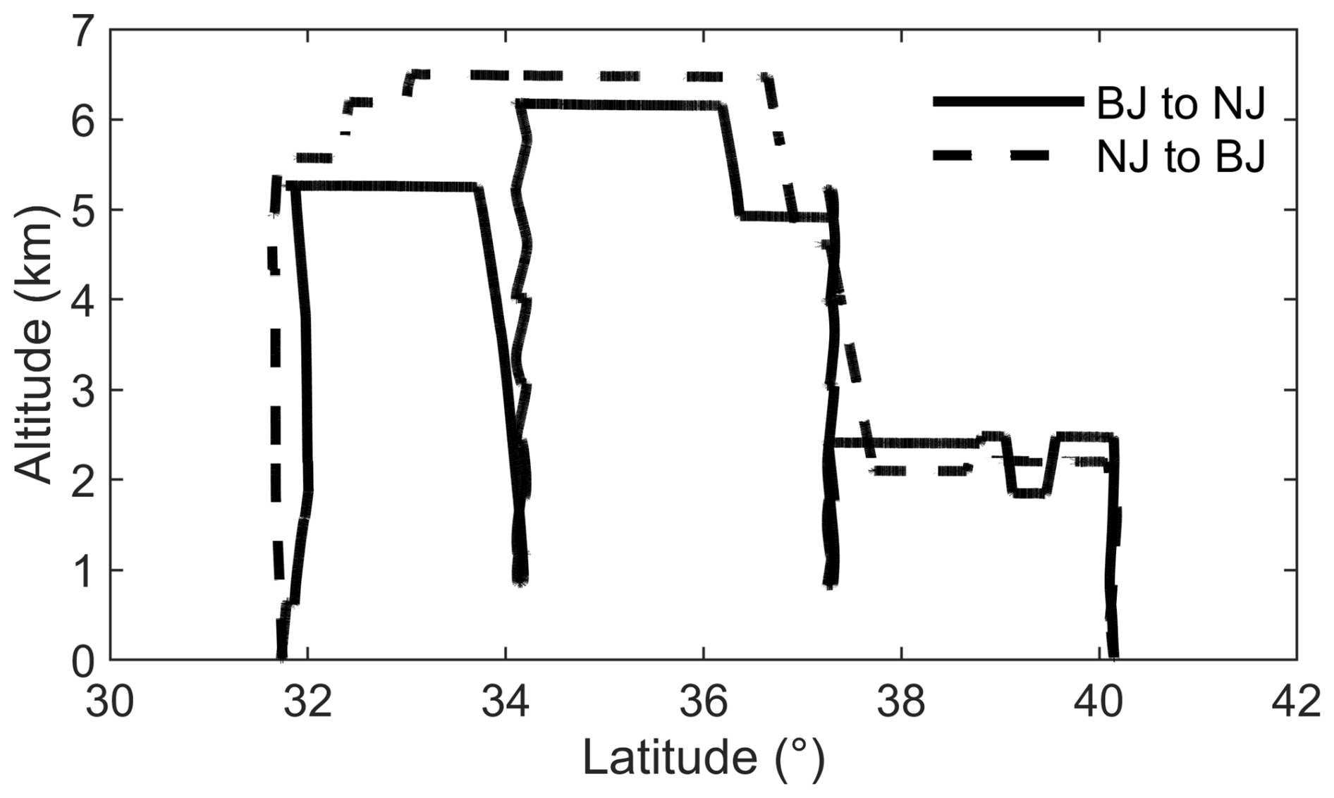
The aircraft took off from Beijing at 09:44 LT Beijing time (about 4 h after sunrise), reached an altitude of 2470 m at 09:49 LT and then flew southward. At 10:57 LT, it started to descend in a spiral pattern from 2410 m to 820 m over Henghui, and then started to ascend at 11:05 LT, reaching an altitude of 6160 m at 11:51 LT and resuming the southward flight. At 12:38 LT, it spiralled down from 6170 to 850 m over Shangqiu. After completing this descent at 13:08 LT, it ascended to an altitude of 5250 m at 13:20 LT and continued its southward flight. It landed in Nanjing at 14:44 LT. The aircraft took off from Nanjing at 18:31 LT, reached an altitude of 550 m at 18:54 LT and continued the northward travel. It started to descend near Beijing from an altitude of 2200 m at 21:15 LT, and landed in Beijing at 22:17 LT. A total of 8 vertical profiles of CO₂ and CH₄ concentrations were obtained. These are denoted as BJ↑, BJ↓, HS↑, HS↓, SQ↑, SQ↓, NJ↑ and NJ↓, with the upward arrow indicating ascent and the downward arrow indicating descent.

A portable CO₂/CH₄/H₂O analyzer based on the off-axis integrated cavity output spectroscopy (model GLA-132-GGA, Los Gatos Research, Mountain View, CA, USA) was used for the airborne observation. It operated in dual modes, one for low pressure and the other for normal atmospheric pressure. The sampling frequency was 1 Hz. Its measurement accuracy was CH₄ < 2 ppb, CO₂ < 0.3 ppm, H₂O < 100 ppm. The analyzer was calibrated before the flight. Calibration of water vapor mixing ratio was performed with a dewpoint generator (LI-610, LI-COR Inc., Lincoln, Nebraska, USA) at dewpoints of 1, 5, 10, 15, and 20 °C. Calibration of CO₂ and CH₄ was made with two working standard gases with CO₂ concentrations of 400 and 600 ppm and CH₄ concentrations of 2000 and 3000 ppb. All working standard gases were calibrated with NOAA standard gases before use.

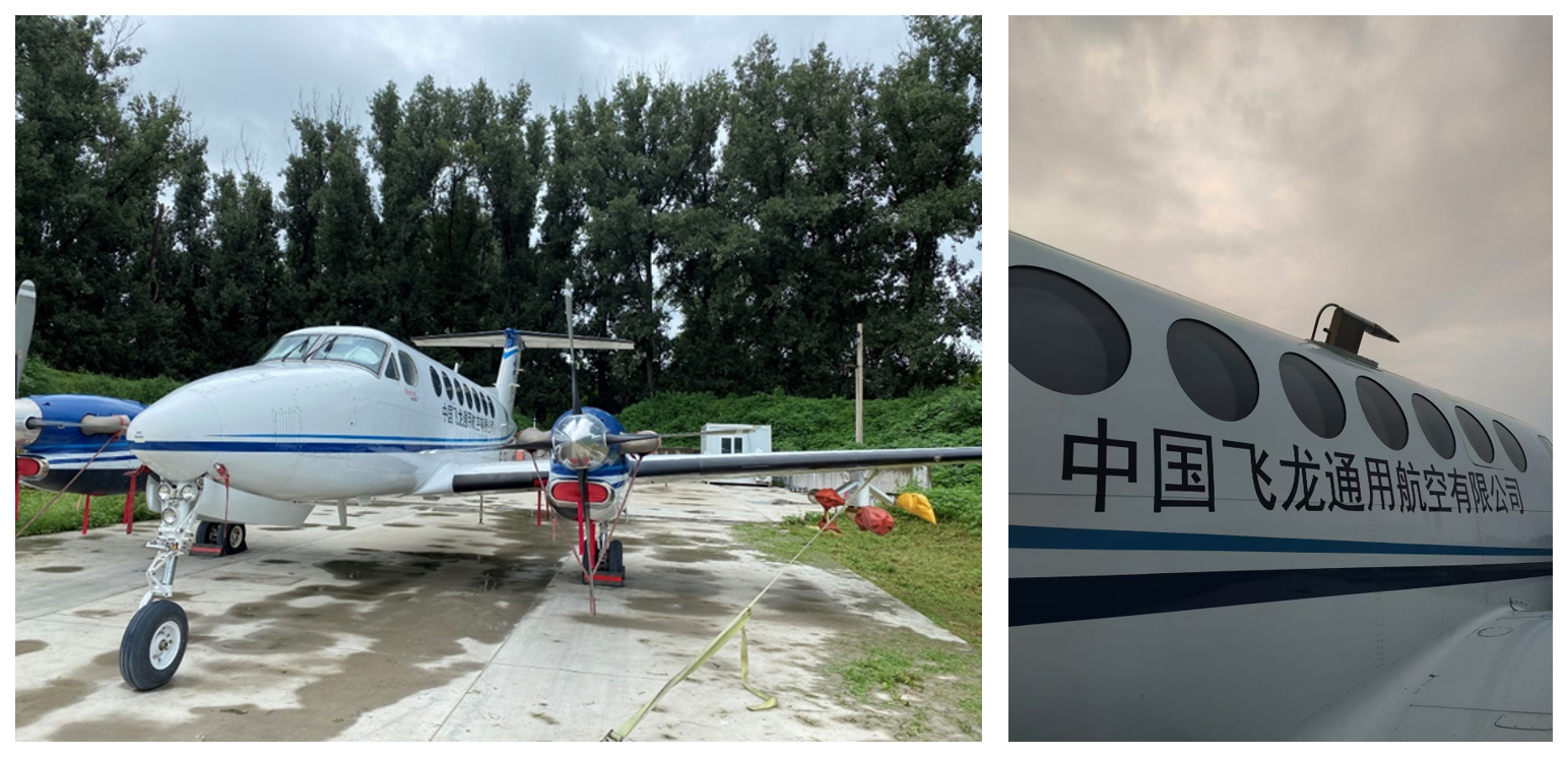
The aircraft (King Air model B3587, Beechcraft Aircraft, Fig. 3) was equipped with an air sampling system, including a gas inlet, an aerosol inlet, an external pump and an exhaust. Air was drawn via a sampling tube (Teflon, outer diameter $\mathrm{1}/\mathrm{4}$ in., length 5.5 m) from the inlet on the top of the aircraft. The inlet was fit with a filter to remove dust particles. The lag time was 1 s. A cold trap was placed upstream of the analyzer to remove most of the moisture in the air sample. The concentration of the residual moisture was measured by the analyzer; this measurement was used to convert the CO₂ and CH₄ concentrations to molar dry mixing ratios.

In parallel to the gas measurement, an Aircraft Integrated Meteorological Measurement System (AIMMS-20, Aventech Inc., Barrie, Ontario, Canada) was used to measure meteorological variables, including air temperature, humidity and pressure. The potential temperature and specific humidity were calculated from the observed temperature, humidity and pressure.

2.2 Mobile ground-based observation in Nanjing

Ground-based atmospheric CO₂ and CH₄ concentrations were observed along three routes in Nanjing around the time when the aircraft landed (Figs. 1 and S1 in the Supplement), using three analyzers (model 915-0011, Los Gatos Research, Mountain View, CA, USA) carried by passenger cars. These analyzers were calibrated before the experiment using the same procedure described above. The air inlet of the analyzer was positioned above the roof of the car, at a height of about 2.5 $\mathrm{m}\mathrm{a}.\mathrm{g}.$ (Hu et al., 2018). Air temperature and air humidity were measured with a Smart-T sensor (Cao et al., 2020) also installed on the top of the car. Route 1 was a 50 km long transect at a distance of about 30 km north of the airport. Measurement started from the west end at 13:00 LT and reached the eastern end at 15:05 LT. The other two routes formed a large and a small loop around the airport, in a near circular pattern with a radius of 8 and 4 km. Measurement on these routes started at 13:0 LT. The large loop (Route 3) was repeated twice, with the measurement ended at 14:23 LT. The small loop (Route 2) was repeated four times, with the measurement ended at 14:56 LT. Observations made on Routes 2 and 3 were used to compute the mean surface values for comparison with the airborne observation.

2.3 Inventory data

The CH₄ : CO₂ emission ratio obtained from airborne observation was compared with the ratio based on the Edgar emission inventory database version 8.0 (https://edgar.jrc.ec.europa.eu/dataset_ghg2024 (last access: 8 April 2025). This is a global inventory product with a spatial resolution of 0.1° × 0.1°. This study uses the inventory data in 2023. First, we calculated the total emission for each city and the corresponding total area within the city administrative boundary. The emission flux ($\mathrm{mg}{\mathrm{m}}^{-\mathrm{2}}{\mathrm{s}}^{-\mathrm{1}}$) was then calculated as the ratio of the total emission to the total area.

3 Results

3.1 Background conditions

According to the surface weather map for 14 May 2023 (Fig. S2), eastern China was under the influence of a high-pressure system in the south (centered at 28° N and 123° E) and a low-pressure system in the north (centered at 35° N and 118° E). The four components of the surface radiation balance indicate that sky conditions at takeoff and landing were partly cloudy in Beijing and clear in Nanjing (Fig. S3). The surface net radiation at noon was 660.1 W m⁻² in Beijing and 655.6 W m⁻² in Nanjing. On the day of airborne campaign, air pollution levels were moderate in Eastern China, with the surface PM_2.5 concentration ranging from 15 to 46 µg m⁻³ (Beijing), 14 to 46 µg m⁻³ (Henghsui), 26 to 42 µg m⁻³ (Shangqiu), and 23 to 47 µg m⁻³ (Nanjing). In Beijing, the surface wind speed was 1.7 m s⁻¹ (from the northeast) at takeoff and 1.9 m s⁻¹ (from the northeast) at landing. In Nanjing, the wind speed was 0.5 m s⁻¹ (from the southwest) at takeoff and 2.3 m s⁻¹ (from the southwest) at landing.

Figure 4 CO₂ and CH₄ concentrations as a function of latitude. Data are 5 min averages.

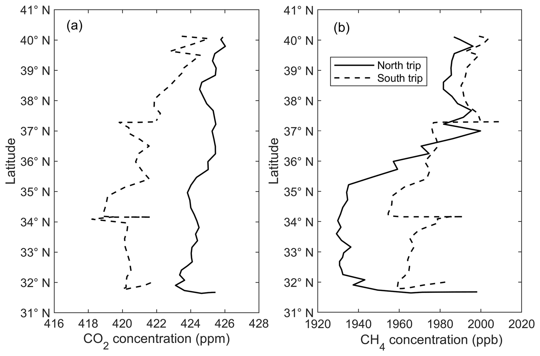
Figure 4 shows the concentrations in the free atmosphere (above 2 km in altitude) as a function of latitude. The overall CO₂ concentration in the south trip (from Beijing to Nanjing) was lower than that in the north trip. The trip mean was 421.0 ± 1.5 ppm for the south trip and 424.6 ± 0.9 ppm for the north trip (from Nanjing to Beijing). These values were 3.3 to 5.3 ppm lower than the concentrations recorded at the WMO surface background sites CPA (Cholpon-Ata, Kyrgyzstan, 42.6369° N, 77.0675° E) and GSN (Gosan, Republic of Korea, 33.29382° N, 126.16283° E) on 14 May 2023 (Fig. S4). These background observations showed higher CO₂ values in the late afternoon and the evening than in the midday, so the difference between the north and the south trip in the free atmosphere appears to partly reflect the CO₂ diurnal trend in this region. For CH₄, the concentration shows a latitude dependence, with higher values in more northern latitudes. The CH₄ concentration was similar between the two trips in areas north of 36.5° N. In areas south of 36.5° N, the CH₄ concentration in the south trip was about 30 ppb higher than that in the north trip. The flight height was similar between the two trips in areas north of 36.5° N, but in areas south of this latitude, the flight height was about 1 km lower in the south trip than in the north trip (Fig. 2), implying a vertical CH₄ gradient of −30 ppb km⁻¹ in the upper troposphere in Eastern China, although some of the difference may have been caused by temporal variations. The trip mean was 1976 ± 15 ppb for the south trip and 1960 ± 26 ppb for the north trip, which were slightly lower than the background concentrations at CPA and GSN (Fig. S4).

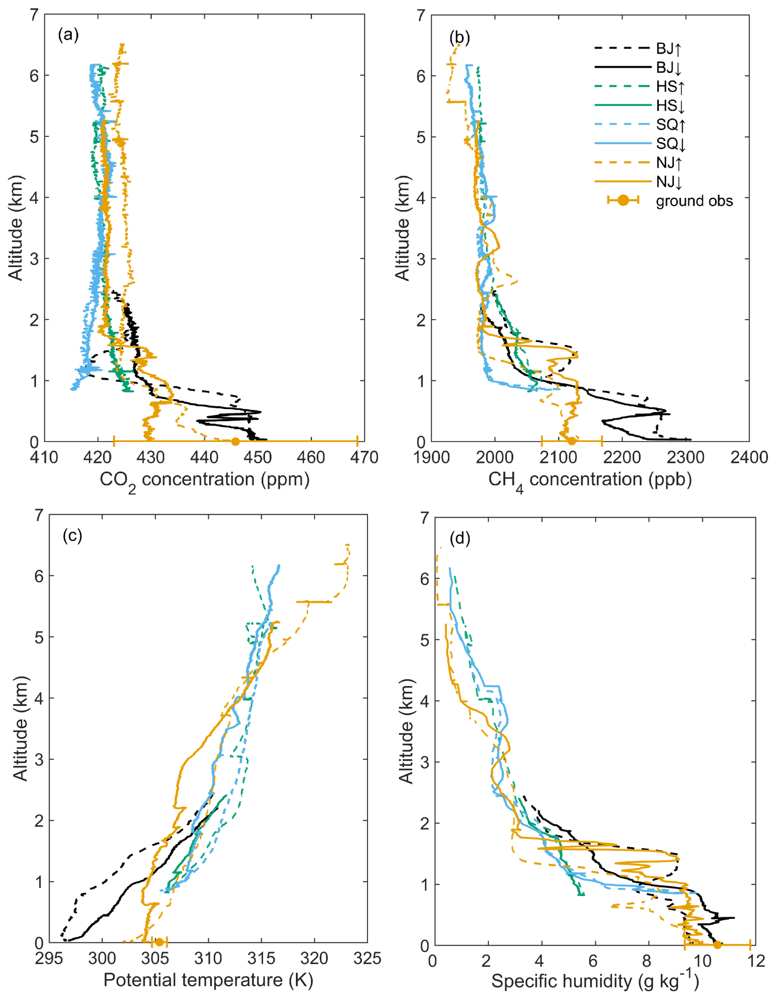
Figure 5 Vertical profiles of atmospheric CO₂ concentration (a), CH₄ concentration (b), potential temperature (c), and specific humidity (d) over the four cities. Yellow dots: ground-based mean values of the vehicle-mounted measurement around the airport in Nanjing. Data points are 1 Hz observations. BJ: Beijing; NJ: Nanjing; HS: Hengshui; SQ: Shangqiu. The wind profiles were presented in Fig. S5.

3.2 Vertical profiles

Figure 5 shows the vertical profiles of CO₂, CH₄, potential temperature, and specific humidity over the four cities. For Beijing and Nanjing, the profiles extended from the free atmosphere down to the surface, while those over Hengshui and Shangqiu extended down to approximately 850 $\mathrm{m}\mathrm{a}.\mathrm{g}.$. Two complete observations were made over Beijing. The ascending profiles of CO₂ and CH₄, observed at about 09:45, indicate the depth of the ABL to be about 800 m. The mean concentrations in the ABL were 447.5 ± 1.6 ppm and 2251 ± 20 ppb for CO₂ and CH₄, respectively. The potential temperature was not well mixed; instead, an inversion layer, at a strength of about 5 K km⁻¹, extended from the 2 km height down to the surface. The specific humidity was more uniform than the potential temperature, changing from 9.5 g kg⁻¹ at the surface to about 8.0 g kg⁻¹ at the top of the ABL. The descending profiles, observed at about 22:12, were still influenced by stable stratification. The ABL at this time was shallower than in the morning, with a depth of approximately 500 m as indicated by the CO₂ profile. The mean concentrations below this height (444.9 ± 3.4 ppm and 2220 ± 34 ppb for CO₂ and CH₄, respectively) were lower than the mid-morning values. The surface humidity increased to 10.8 g kg⁻¹.

Two complete sets of profiles were also obtained over Nanjing. The descending profiles were observed at approximately 14:35 LTThe CO₂, CH₄ and specific humidity profiles indicate that the ABL height was about 1500 m. The potential temperature was more uniform than in the Beijing ABL, showing near neutral to slightly stable stratification. The mean ABL concentrations were 431.0 ± 1.6 ppm and 2120 ± 11 ppb for CO₂ and CH₄, respectively. For comparison, the ground-based concentrations, averaged over Routes 2 and 3 (Fig. S1, the two loops around the airport), were 445.8 ± 22.8 ppm and 2124 ± 41 ppb for CO₂ and CH₄, respectively. The ground-based temperature and specific humidity were slightly greater (by 0.8 K and 1.3 g kg⁻¹) than the surface values observed at the airport by the airborne instruments. The ascending profiles were observed at about 18:31 LT. By this time a surface inversion layer had developed. Although the surface CH₄ at the airport did not change much from that at landing, the surface CO₂ increased to 444.6 ppm at takeoff from 429.6 ppm at landing.

The ground-based CO₂ concentration in Nanjing was 14.8 ppm higher than the average concentration in the ABL at landing, and the CH₄ concentration was 4 ppb higher. These differences might be indicative of strong concentration gradients near the ground. The vehicle-mounted observation was made at 2.5 m a.g. In comparison, the minimum altitude of the aircraft observation exceeded 20 m. Gao et al. (2018) reported that under low wind conditions, a CO₂ concentration difference up to 40 ppm can develop over a vertical separation of 30 m in the surface air layer in Nanjing. Another reason might be that the CO₂ concentration measured on the routes around the airport (Fig. 1) was higher due to stronger traffic influence than at the airport.

The ABL in Beijing in the mid-morning was more enriched in CO₂ and CH₄ than the ABL in Nanjing in the mid-afternoon. The differences in the mean ABL concentrations were 16.5 ppm and 131 ppb for CO₂ and CH₄, respectively. At night, the CO₂ and CH₄ concentrations in Beijing were also higher than those in Nanjing by 9.4 ppm and 114 ppb, respectively. The ABL specific humidity was similar between the two cities. Both cities were net sources of CO₂ and CH₄, despite having high fractions of urban greenspaces (50 % and 45 % for Beijing and Nanjing, respectively).

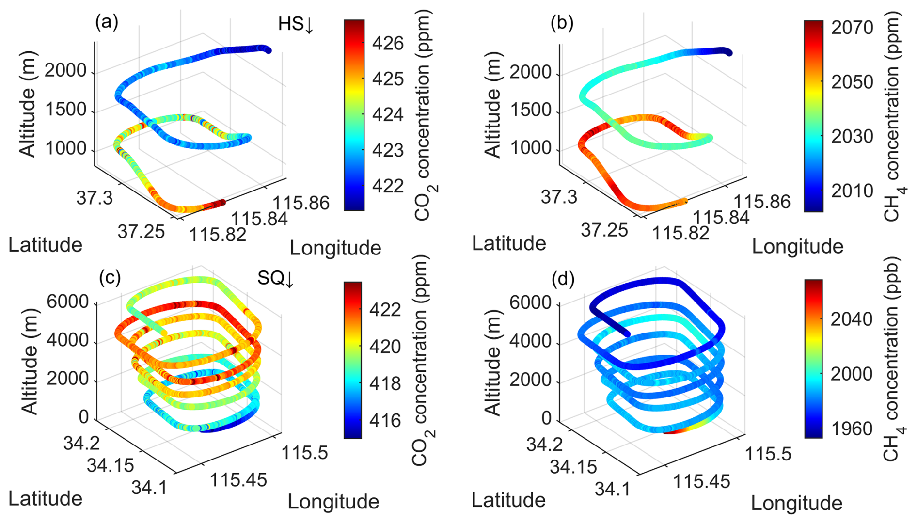
Figure 6 Profiles of CO₂ and CH₄ over Hengshui (top) and Shangqiu (bottom) measured along downward spiral flight paths.

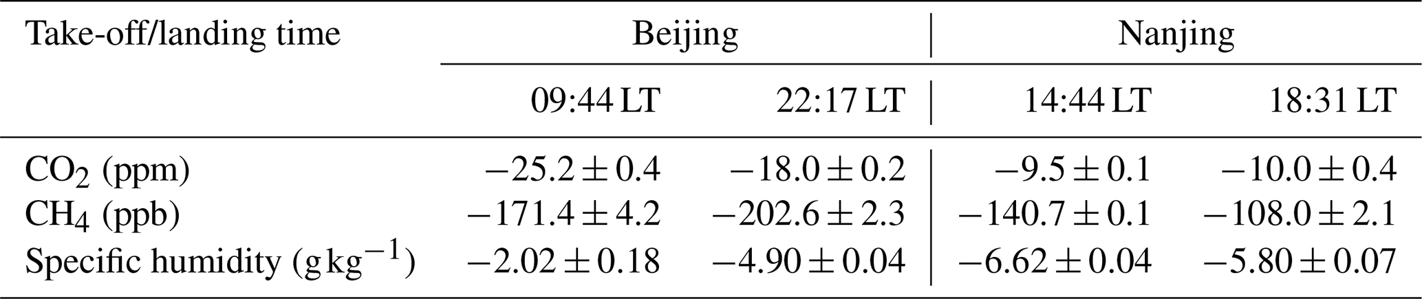
Table 1 Inversion jumps of specific humidity, CO₂ and CH₄ over Beijing and Nanjing.

The profiles over Hengshui and Shangqiu were stopped at 850 $\mathrm{m}\mathrm{a}.\mathrm{g}.$ and did not adequately sample the interior of the ABL. Nevertheless, they indicated that the surface influences on the ABL GHG budgets differed between the two locations. Over these two cities, the ascending and descending CO₂ and CH₄ profiles were nearly identical. The CO₂ concentration showed a decreasing trend with decreasing altitude at Shangqiu, indicating that the surface was a sink of CO₂, whereas it showed an increasing trend with decreasing altitude at Hengshui, indicating the surface was a source of CO₂. The CH₄ concentration showed an increasing trend with decreasing altitude at both locations, reflecting the fact that the surface was a source of CH₄. The CH₄ concentration experienced a rapid change at Shangqiu, increasing from 1998 ppb at 1000 m to 2102 ppb at 850 m. This step-like change suggests that the capping inversion of occurred between 850 and 1000 $\mathrm{m}\mathrm{a}.\mathrm{g}.$ at Shangqiu. A sharp change in specific humidity was also observed between 850 and 1000 m at Shangqiu (Fig. 5d). At an altitude of 850 m, the CH₄ concentration reached a high value of 2102 ppb (nearly the same as the mid-afternoon ABL mean in Nanjing), suggesting that the CH₄ concentration in the ABL at Shangqiu might have been quite high. In other words, the landscape near Shangqiu might be a sink of CO₂ but a strong source of CH₄, and the landscape near Hengshui might be a source for both CO₂ and CH₄. Given the lack of ABL sampling, the exact CO₂ and CH₄ concentration in the ABL at Hengshui and Shangqiu remained unknown.

The spiky appearance of the descending profiles at Hengshui and Shangqiu in Fig. 6 was a consequence of the spiral flight pattern, which mixed horizontal variations with vertical variations (Fig. 6). At Hengshui, the downward spiral started at the altitude of 2413 m and consisted of two loops with the north-south extent of 10 km and the east-west extent of 5.5 km. At Shangqiu, the spiral started at the altitude of 6170 m and consisted of six loops with the north-south extent of 13 km and the east-west extent of 6.5 km. Generally, the CO₂ and CH₄ concentrations exhibited greater variations in the vertical direction than in the horizontal directions. The horizontal variation in CO₂ was about 3 ppm across the spiral loop at the height of about 1.3 km over both cities. In the profile plot in Fig. 6a, the data collected in the horizontal flights were collapsed to the same altitudes, giving the appearance of small horizontal spikes (with a spike length of about 3 ppm). The CH₄ concentration had no discernible horizontal variation at this height, and it showed a small horizontal variation of about 10 ppb at an altitude of about 4 km over Shangqiu (Fig. 6d).

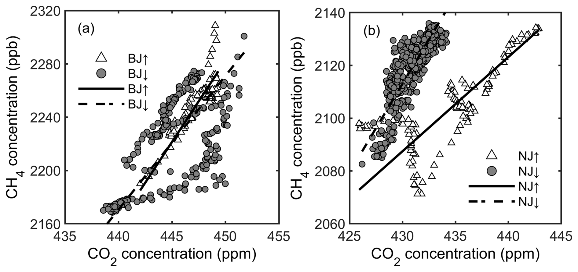
Figure 7 Correlation between CO₂ and CH₄ concentrations in the ABL (a: Beijing; b: Nanjing). Each data point represents 1 s sampling.

3.3 Inversion jumps

Table 1 summarizes the capping inversion jump values of CO₂, CH₄, and specific humidity in Beijing and Nanjing. The actual capping inversion was not visible in the potential temperature profile because of the slow time response of the temperature sensor (The thermistor responds in under a second, but during climb or descent its effective response can stretch to several seconds to about a minute). To determine the jump values, we calculated the average concentrations below 800 m for the midday observation and 500 m for the nighttime observation over Beijing, and below 1500 m for the mid-afternoon observation and 1000 m for the early evening observation over Nanjing, to represent the concentrations in ABL. The average concentration in the 1–2 km layer over Beijing and that in the 2–3 km layer over Nanjing was used as the average concentration of the lower free atmosphere. The difference between the average concentration in the ABL and that of the free atmosphere was taken as the inversion jump. For CO₂, the inversion jump value in Beijing was −25.2 ± 0.4 ppm in the mid-morning and −18.0 ± 0.2 ppm at night, indicating a larger vertical gradient during the day. In Nanjing, the CO₂ inversion jump value was −9.5 ± 0.1 ppm in mid-afternoon and −10.0 ± 0.4 ppm in the early evening, showing an opposite trend to Beijing. For CH₄, the inversion jump value in Beijing increased slightly in magnitude with time, from −171.4 ± 4.2 ppb in the mid-morning to −202.6 ± 2.3 ppb at night. A decreasing magnitude was observed in Nanjing, where the CH₄ inversion jump value changed from −140.7 ± 0.1 ppb in the mid-afternoon to −108.0 ± 2.1 ppb in the early evening. For specific humidity, the inversion jump in Nanjing was higher in magnitude than in Beijing.

3.4 CH₄ and CO₂ correlation

Figure 7 shows the correlation between CO₂ and CH₄ concentrations in the ABL in Beijing and Nanjing. A highly significant correlation was observed between the concentrations of the two gases in both cities (p < 0.01). In Beijing, the data collected during the mid-morning take-off (ascending) and during the evening landing (descending) were clustered together. The mid-morning regression slope was 12.22 ppb ppm⁻¹, with a correlation coefficient (r) of 0.87. At night, the slope decreased to 10.03 ppb ppm⁻¹, and r was 0.65. The Nanjing data showed a clear separation between takeoff and landing, with lower CO₂ and CH₄ concentrations at landing (descending) in the mid-afternoon than at takeoff (ascending) in the early evening. The midafternoon regression slope was 6.71 ppb ppm⁻¹ with an r value of 0.83, while the early evening slope was 3.57 ppb ppm⁻¹ with an r of 0.78. The regression slopes for Beijing were nearly twice those observed in Nanjing, reflecting a stronger urban CH₄ source in Beijing (Sect. 4.1). The correlation between the two gases were stronger for Nanjing than for Beijing, probably because the ABL was better developed in Nanjing. In comparison, the free-atmospheric ratio over Beijing and Nanjing diverged significantly (Fig. S6).

The two gases were highly correlated in the free atmosphere (altitude greater than 2 km; Fig. 8). The correlation was significant for both trips (r > 0.73, p < 0.001). The data during these two trips form two distinct clusters. The regression slope of the south trip was 10.01 ppb ppm⁻¹, which falls between the free tropospheric values observed over Hengshui and Shangqiu (Fig. S7). The regression slope of the north trip was much higher, at 29.95 ppb ppm⁻¹.

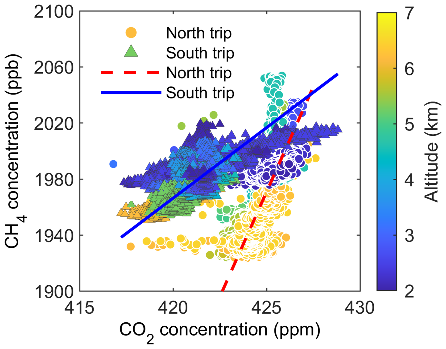
Figure 8 Correlation between CO₂ and CH₄ concentrations above 2 km. Data points are 1 Hz observations.

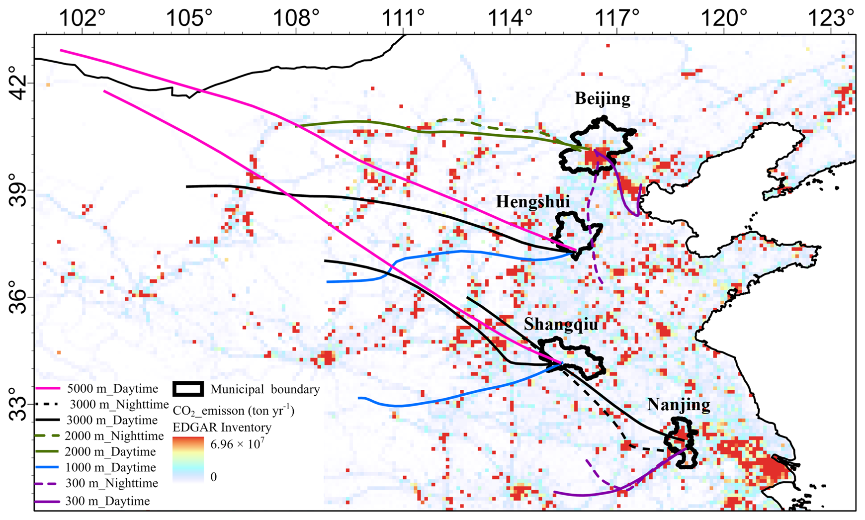
Figure 9 Backward trajectories of air mass at different end heights. Background map shows the EDGAR CO₂ emission inventory with the color scale indicating annual emission amount per 0.1° by 0.1° grid. Trajectory length is 24 h.

4 Discussion

4.1 Contrasts among the four cities

We compared the EDGAR emission inventory data with the observed concentration profiles. The CO₂ and CH₄ concentrations in the four cities were inconsistent with the inventory products. The EDGAR CO₂ emission flux of the four cities was, in order from the highest to the lowest, Nanjing (0.58 $\mathrm{mg}{\mathrm{m}}^{-\mathrm{2}}{\mathrm{s}}^{-\mathrm{1}}$), Beijing (0.16 $\mathrm{mg}{\mathrm{m}}^{-\mathrm{2}}{\mathrm{s}}^{-\mathrm{1}}$), Shangqiu (0.11 $\mathrm{mg}{\mathrm{m}}^{-\mathrm{2}}{\mathrm{s}}^{-\mathrm{1}}$) and Hengshui (0.058 $\mathrm{mg}{\mathrm{m}}^{-\mathrm{2}}{\mathrm{s}}^{-\mathrm{1}}$). However, the CO₂ concentration in Beijing was much higher than that in Nanjing, and the concentration at 850 m (the lowest observation altitude) in Hengshui was also higher than that in Shangqiu. For CH₄, the emission flux order was Nanjing (1.35 $\mathrm{\mu }\mathrm{g}{\mathrm{m}}^{-\mathrm{2}}{\mathrm{s}}^{-\mathrm{1}}$), Beijing (0.67 $\mathrm{\mu }\mathrm{g}{\mathrm{m}}^{-\mathrm{2}}{\mathrm{s}}^{-\mathrm{1}}$), Shangqiu (0.56 $\mathrm{\mu }\mathrm{g}{\mathrm{m}}^{-\mathrm{2}}{\mathrm{s}}^{-\mathrm{1}}$) and Hengshui (0.32 $\mathrm{\mu }\mathrm{g}{\mathrm{m}}^{-\mathrm{2}}{\mathrm{s}}^{-\mathrm{1}}$). But again, the CH₄ concentration in Beijing was higher than that in Nanjing. These contrasts urge caution against using the concentrations as indication of emission strengths. We note that the profiles in Fig. 5 were sampled at different times of the day. Some of the differences may have been caused by changing atmospheric conditions. The general inter-city patterns were unaffected because the temporal differences in the concentrations sampled at takeoff and at landing were smaller than the between-city differences.

Four possible factors might account for the discrepancies between the emission inventory data and the concentrations in Beijing and Nanjing. One possible reason was spatial heterogeneity of the surface emission sources. In Nanjing, the CO₂ and CH₄ emission inventories included four and three grids with abnormally high emission values, respectively. These grids, located at 30 to 60 km to the north of the airport, were missed by the air trajectory arriving in the ABL in Nanjing (Figs. 9 below and S8). After removing these grids, the CO₂ and CH₄ emission fluxes in Nanjing decreased to 0.22 $\mathrm{mg}{\mathrm{m}}^{-\mathrm{2}}{\mathrm{s}}^{-\mathrm{1}}$ and 1.13 $\mathrm{\mu }\mathrm{g}{\mathrm{m}}^{-\mathrm{2}}{\mathrm{s}}^{-\mathrm{1}}$, respectively. The CO₂ emission flux was only about 38 % of the original value, and the CH₄ emission flux also decreased accordingly. The second possible reason was the difference in mixing efficiency in the ABL. The ABL height in Beijing was approximately half that in Nanjing, which would result in higher average concentrations in the Beijing ABL. The third reason was the difference in vegetation photosynthetic efficiency. Although the NDVI in Beijing (0.54) was similar to that in Nanjing (0.53) during the experimental period, the growing season was still early in in Beijing and the plant photosynthetic uptake of CO₂ was likely lower than that in Nanjing. The fourth possible reason was advection. As an air mass moves, it continuously accumulates emissions from the surface along its path, leading to higher concentrations in downwind areas. More CO₂ might have been accumulated near the surface in Beijing than in Nanjing. Overall, these four factors might explain the lack of agreement between the emission inventory and the observed concentrations.

4.2 Influence of airmass trajectories

In the idealized one-dimensional urban boundary layer, the CO₂ and CH₄ emitted by sources in the city are trapped in a dome above the city. Their vertical profiles and time changes are shaped by the surface emission, vertical mixing and exchanges with the free atmosphere. Horizontal advection does not play a role. In this study, the ABL deviates from this idealization because the vertical concentration profiles were also influenced by airmass advection. Figure 9 illustrates the sources of air mass at different altitudes in each city. In Fig. 9, the basemap shows the EDGAR CO₂ emission flux. The same trajectories are also plotted against the EDGAR CH₄ emission map (Fig. S8). The concentrations within the ABL in Beijing and Nanjing were influenced by short-range transport and local emissions. In Beijing, the daytime air mass trajectory passed through high-emission areas located to the southwest of the city, whereas at night, few high-emission areas were present along the trajectory. This pattern was consistent with the higher CO₂ and CH₄ concentrations at the height of around 300 m in the daytime than at night (Fig. 5a and b).

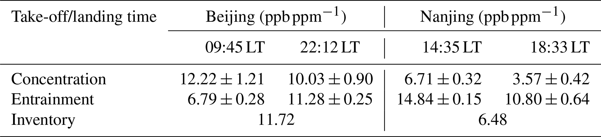
Table 2 CH₄:CO₂ emissions ratios obtained with the ABL concentration data, the inversion jump values and the EDGAR inventory data.

In Nanjing, the backward trajectories in the ABL at landing and at take-off were similar. The observed higher CO₂ concentration at the evening take-off (Fig. 5a) might have been caused by accumulation of locally-emitted CO₂ in the ABL. Interestingly, the CH₄ concentration near the surface experienced little change between these two times. It appears that at the evening takeoff, the CO₂ concentration was influenced heavily by vehicle emissions near the airport, whereas the CH₄ concentration was influenced by more distance sources such as landfills. This is a reason for why the ABL data for Nanjing in Fig. 7 exhibits two distinct clusters for the takeoff and landing.

In the free atmosphere, the GHG concentrations were mainly controlled by long-range air mass transport. The CO₂ concentration above 3 km in Nanjing was about 3 ppm higher at takeoff than at landing (Fig. 5a). The backward trajectories indicate that during landing, the air mass passed over regions with relatively low CO₂ emissions (Fig. 9). At takeoff a few hours later, the air mass passed through Huainan, a city with intensive energy and chemical industries, and Hefei, the provincial capital of Anhui Province. The variation in air mass trajectories also resulted in changes in the ratios above Hengshui and Shangqiu (Fig. S7).

Previous studies have similarly concluded that advection of airmass exert a large influence on GHG concentrations. Airmass trajectory patterns are responsible for synoptic-scale variability of CO₂ and CH₄ concentrations at a regional background site on the west coast of South Korea (Kenea et al., 2023). Liu et al. (2025) presented two AirCore profiles of CO₂ over Hangzhou, a city about 200 km to the southeast of Nanjing, with one influenced by northeasterly flow and the other by southeasterly flow. The second profile shows consistently higher concentration by about 3 ppm than the first profile between the 2 and 25 km altitude, a difference similar to that we observed between take-off and landing in Nanjing (Fig. 5a). In an airborne field campaign over Bhubaneswar, Varanasi and Jodhpur of India, Sreenivas et al. (2019) observed that high CO₂ concentration below the 1 km altitude is associated with northwesterly flow. Umezawa et al. (2016) reported that the CO₂ concentration observed by an CONTRAIL aircraft over Delhi, India shows decreasing trends towards the ground on some days and increasing trends on other days; these fluctuations were associated with synoptic weather conditions that presumably altered airmass trajectories and therefore the relative roles of CO₂ uptake by the cropland near the city and CO₂ emission in the city. In an expanded analysis of the CONTRAIL data, Umezawa et al. (2020) showed that the CO₂ concentration at 1.0–1.5 km altitude is enhanced than the background by 1 to 6 ppm if the airmass trajectory passes a major city. They also reported that this local urban influence on the CO₂ concentration between the 4.0 and 4.5 altitude is weaker.

4.3 CH₄ : CO₂ ratio

The CH₄ : CO₂ ratio in the ABL can serve as an independent check on the accuracy of emission inventories. Table 2 compares the ratios determined with the concentration observations and those with inventory data. According to the EDGAR inventory data, the CH₄ : CO₂ emissions ratio was 11.72 ppb ppm⁻¹ for Beijing and 6.48 ppb ppm⁻¹ for Nanjing. To minimize the influence of photosynthetic CO₂ uptake, we compared these with the aircraft-observed ratios at night. Results showed that the inventory ratio was within the measurement uncertainty in Beijing and was higher by about 80 % in Nanjing. Several factors may have contributed to the mismatch in Nanjing. First, vehicle and waste management are the two major CH₄ emission sources in Nanjing. In the last decade, vehicle fleets in Chinese cities have experienced two shifts in fuel use, first from gasoline to natural gas and then from gasoline and natural gas to electric (Hao et al., 2016; China's Energy Transition, 2024). These transitions were not accounted for by the EDGAR inventory. Second, using an inversion modeling with CH₄ concentration data, Hu et al. (2023) estimated that EDGAR CH₄ emission in Hangzhou is biased high by about 50 % primarily due to a high bias for the waste management sector. It is possible that this source category was also biased high for Nanjing because Nanjing and Hangzhou, both located in the YRD, use similar methods to manage waste. Third, residents in Nanjing use natural gas for space heating. The inventory data are annual mean values that include contributions from space heating, whereas the aircraft observation was made in late spring when space heating was no longer needed. Finally, this study used the nighttime concentration ratio for comparison, an approach that can reduce, but not eliminate, the influence of the biosphere on CO₂. Addition of a typical respiration CO₂ flux of 0.1 $\mathrm{mg}{\mathrm{CO}}_{\mathrm{2}}{\mathrm{m}}^{-\mathrm{2}}{\mathrm{s}}^{-\mathrm{1}}$ to the EDGAR CO₂ emission would reduce the inventory emissions ratio in Nanjing to 5.46 ppb ppm⁻¹. The relative roles of these factors cannot be inferred from one profile sampling, and a firm conclusion will require more observational data, a better estimate of biospheric respiration, and allocation of the annual inventory total to seasons and daytime and nighttime.

Table 2 also presents the ratio of the CH₄ to the CO₂ entrainment flux at the ABL top. Since the entrainment velocity is the same for both gases, the entrainment flux ratio is equivalent to the ratio of the inversion jump values shown in Table 1. This flux ratio was close to the ratio derived from the ABL concentration data in Beijing at night, but it was lower than the ABL ratio during the day. In Nanjing where the ABL was well developed, the entrainment flux ratio was much greater than the ABL ratio at both times. These results suggest that the one-dimensional slab approximation (Chapter 11; Lee, 2023) may be too simplistic for the urban ABL. In this approximation, there is no advective influence. Using large-eddy simulations, Huang et al. (2011) showed that in a fully developed one-dimensional ABL under steady state, the entrainment CO₂ flux is approximately equal to the surface CO₂ flux. This equality should also hold for CH₄ because like CO₂, CH₄ is conserved trace gas and without a source or sink above the ABL, implying equality of the CH₄:CO₂ flux ratio at the surface and at the ABL top. However, in an evolving ABL, the surface and the entrainment CO₂ flux can be quite different (Vilà-Guerau de Arellano et al., 2004). Furthermore, as air moves from the rural background into the urban domain, its CH₄ and CO₂ concentrations will increase with downwind distance (Gao et al., 2018). This advection contribution to the urban ABL GHG budgets was likely important. An analogous situation exists in the European Arctic wetlands, where the ABL air becomes gradually enriched in CH₄ and depleted in CO₂ as it moves across the region (O'Shea et al., 2014), but unlike the urban land in Nanjing where the surface was a net source of both CO₂ and CH₄, these wetlands are a source of CH₄ and a sink of CO₂.

In the free atmosphere, the ratio obtained during the north trip was about three times that during the south trip (Fig. 8). The observed difference is likely caused by the difference in flight altitude. In latitudes between 33.0 and 36.5° N, the airplane flew at a cruising altitude of 6.5 km during the north trip, which was 0.5 to 1.3 km greater than during the south trip. At this altitude, the CH₄ concentration was lower than at lower altitudes (Fig. 4b). If we exclude the data obtained above 5.5 km, the data collected during the two trips would collapse to a similar clustering pattern (Fig. 8).

4.4 Inversion jumps

The CO₂ and CH₄ inversion jumps reveal information about the role of entrainment at the ABL top. The entrainment flux is proportional to the jump value. If the jump value is positive ((higher concentration in the free atmosphere than in the ABL), entrainment will enrich the gas in the ABL. If the jump value is negative (lower concentration in the free atmosphere), entrainment will deplete the gas in the ABL.

Our study appears to be the first to report the CO₂ and CH₄ inversion jumps in the urban ABL. Unlike previous studies targeting concentrations in urban plumes or in the urban surface layer, this study directly observed the vertical structures of CO₂ and CH₄ above cities. Crawford et al. (2016) and Li et al. (2014) obtained CO₂ profile data in the ABL in Vancouver, Canada and Xiamen, China, respectively, using tethersondes, but their analyzers did not have enough precision and fast enough time response to resolve the sharp CO₂ concentration change across the capping inversion. Our inversion jump values were negative for both daytime and nighttime, indicating the dominant contributions of anthropogenic emissions to the urban ABL CO₂ and CH₄ budgets. The CO₂ inversion jump reported by other authors for vegetated landscapes can be negative (higher CO₂ concentration in the ABL) or positive (higher CO₂ concentration in the free atmosphere), depending on time of the day. For example, Lloyd et al. (2001) reported a CO₂ inversion jump of about +10 ppm above a forest and wetland mosaic in central Siberia in the mid-afternoon. Vilà-Guerau de Arellano et al. (2004) observed a CO₂ inversion jump of −20 ppm above a cropland landscape in the early morning. Several studies have reported the CH₄ profile with large enough vertical span over the full ABL (Barker et al. 2021; Filges et al., 2015; Hartery et al., 2018; Narbaud et al., 2023; O'Shea et al., 2014); Generally, the CH₄ inversion jump in these profiles is too weak and cannot be determined precisely. One exception is Hartery et al. (2018), who showed a profile over the Alaskan permafrost region with a CH₄ inversion jump of about −10 ppb, which is smaller by an order of magnitude than the values given in Table 1.

5 Summary and future outlook

The airborne experiment yielded CO₂ and CH₄ concentration data in the ABL over four cities (Beijing, Hengshui, Shangqiu, and Nanjing) and in the free atmosphere (2.0 to 6.5 km above the sea level) in Eastern China. Based on the observations, four key results are summarized as follows:

Complete vertical profiles in Beijing and Nanjing: the concentrations of CO₂ and CH₄ were higher in the ABL than those in the free atmosphere. In Beijing, the CO₂ inversion jump value was −25.2 ± 0.4 ppm at takeoff in the mid-morning (09:45 Beijing time) and −18.0 ± 0.2 ppm at landing in the evening (22:12). In Nanjing, the jump value was −9.5 ± 0.1 ppm at landing in the afternoon (14:35) and −10.0 ± 0.4 ppm at takeoff in the early evening (18:33). For CH₄, the inversion jump in Beijing were −171.4 ± 4.2 ppb at takeoff and −202.6 ± 2.3 ppb at landing, while in Nanjing it was −140.7 ± 0.1 ppb at landing and −108.0 ± 2.1 ppb at takeoff.

Partial vertical profiles in Hengshui and Shangqiu: In its spiral descent, the airplane detected variations of about 3 ppm in CO₂ and 0 to 10 ppb in CH₄ over horizontal distances of 5.5 to 13 km in the free atmosphere above the ABL. Below the height of 3 km, the two concentrations were positively correlated in Hengshui and negatively correlated in Shangqiu, indicating that the landscape in Hengshui was a CO₂ source and that in Shangqiu was a CO₂ sink.

CH₄:CO₂ ratio: The CH₄:CO₂ emissions ratio inferred from the nighttime ABL concentration data was within the measurement uncertainty in Beijing and was higher by about 80 % in Nanjing. One possible reason is that the inventory did not account for the recent energy transition from gasoline and natural gas to electric in the transport sector. The emissions ratio measured in the well-developed ABL in Nanjing was only about half of the ratio of the CH₄ to CO₂ entrainment flux at the ABL top, calling into question about the suitability of the one-dimensional slab approximation for the urban ABL.

Concentrations in the free atmosphere: The mean CO₂ concentration during the evening flight from Nanjing to Beijing was 3.6 ppm greater than the mean concentration during the daytime flight from Beijing to Nanjing. In terms of CH₄, the concentration showed latitude and altitude dependence, with higher values in more northern latitudes and at lower altitudes. In latitudes between 32.0° and 36.5° N, the concentration difference between the south and the north trip implies a vertical CH₄ gradient of −30 ppb km⁻¹ in the upper troposphere.

In this paper, we focused on the CO₂ and CH₄ characteristics in the urban boundary layer. The dataset accompanying this paper can also be used for validation of satellite retrievals and atmospheric transport models (Liu et al. 2025; Sreenivas et al., 2019). Our results suggest that the simple one-dimensional slab model of the convective ABL may be inadequate for describing GHG budgets in the urban environments. An alternative is the advection-entrainment-diffusion model described by Lee (2023; Chapter 12). This model requires observing variations in both the vertical and the horizontal directions.

Future airborne missions should consider a spiral descent or ascent flight pattern over the target city, but unlike the patterns shown in Fig. 6, it should be extended to the lower portion of the ABL. This measurement strategy would yield information on both the ABL vertical structure and horizontal gradients in the ABL. Instead of sampling multiple cities, repeated profiles over time at the same city would allow better evaluation of the ABL dynamics and entrainment influence. Furthermore, winter season is preferred to reduce the confounding effect of biological fluxes.