Improved isoprene emission estimates over the Finnish boreal forest using the MEGANv3.2 model

In this study, we present an improved framework for modelling isoprene emissions based on the latest version of the Model of Emissions of Gases and Aerosols from Nature (MEGAN). We use high-resolution domain-specific tree cover data, species distributions, and species-specific emission factors to update isoprene emission factors tailored to the Finnish boreal region. These modifications are implemented in MEGAN and integrated into the WRF-CHIMERE chemistry transport model, enabling a more accurate simulation of biogenic emissions. We perform simulations over three consecutive summer periods for the years 2017, 2018, and 2019. Our results reveal a significant reduction in bias for both isoprene emissions fluxes and concentrations compared to previous versions of MEGAN. We further evaluate a canopy correction model to account for the effects of forest canopy on vertical and horizontal transport of biogenic volatile organic compounds (BVOCs). These adjustments further reduce the bias in modelled isoprene concentrations. The enhanced representation of isoprene emissions and the effects of canopy on dispersion processes both result in overall improvements (although small) in SOA formation and transport. Our findings highlight the importance of moving beyond broad vegetation categories and incorporating detailed tree species distributions in emission factor calculations, demonstrating that ecosystem-specific adjustments are essential for realistic modelling of biogenic emissions and their impacts on atmospheric chemistry.

1 Introduction

Forests significantly affect atmospheric composition by emitting and removing a multitude of gases and aerosol particles (Fowler et al., 2009). Among emissions, biogenic volatile organic compounds (BVOCs) play a crucial role in the atmospheric chemistry and physics, influencing ozone (O₃) production, secondary organic aerosol (SOA) formation, and ultimately the climate (Seinfeld and Pandis, 2016). It is estimated that globally, BVOCs emissions account for over 90 % of the total volatile organic compounds (VOCs) emissions (Wang et al., 2024b). Around 70 % of BVOCs emissions are thought to be produced from tropical trees, while only 3 % originate from boreal trees (Guenther et al., 2012). Despite this relatively low contribution arising from boreal forests, previous studies have shown that biogenic SOA originating from the boreal region can affect cloud properties and the climate (Tunved et al., 2006; Paasonen et al., 2013; Yli-Juuti et al., 2021; Petäjä et al., 2022).

BVOCs consist of thousands of different compounds (Peñuelas and Staudt, 2010), among which the most studied and most abundant in the atmosphere are isoprene (C₅H₈) and monoterpenes (C₁₀H₁₆, e.g. α-pinene, β-pinene, limonene) (Guenther et al., 1995; Laothawornkitkul et al., 2009). Isoprene emissions are estimated to range from 299 to 594 Tg C yr⁻¹, accounting for 41 %–70 % of the global BVOCs emissions, while monoterpenes emissions estimations range from 63 to 184 Tg C yr⁻¹, corresponding to 10 %–22 % of the global BVOCs emissions budget (Arneth et al., 2011; Guenther et al., 2012; Messina et al., 2016; Sindelarova et al., 2014, 2022; Weng et al., 2020; Opacka et al., 2021; Wang et al., 2024a). Isoprene is removed from the atmosphere primarily through its reaction with the OH radical, resulting in a lifetime of about 1.4 h under typical OH levels (2×10⁶ molecule cm⁻³). On a global scale, this pathway accounts for approximately 85 % of the total isoprene sink, while oxidation by O₃ and NO₃ accounts for about 9 % and 5 %, respectively (Müller et al., 2019). Although isoprene can react efficiently with the NO₃ radical, the absence of night-time isoprene emissions makes this pathway overall less important (Atkinson, 2000; Seinfeld and Pandis, 2016). On the other hand, monoterpenes can react rapidly with all the atmospheric oxidants; OH, O₃, and NO₃, with night-time oxidation also relevant due to non-zero monoterpenes emissions during night (Laffineur et al., 2011; Hakola et al., 2017). The products of the oxidation of these BVOCs are organic gases with lower saturation vapour concentration (C^*). These gases can have C^* low enough to transition into the aerosol phase, effectively contributing to new particle formation and aerosol growth (Ehn et al., 2014; Riccobono et al., 2014; Lehtipalo et al., 2018; Bianchi et al., 2019).

Isoprene and monoterpenes contribute to SOA formation with different efficiencies. Previous studies have reported SOA yields for isoprene ranging between 0 %–5 % (Edney et al., 2005; Kroll et al., 2006; Ng et al., 2006; Kleindienst et al., 2006; Dommen et al., 2006), showing that, under typical atmospheric conditions, isoprene is not an efficient source of SOA. Monoterpenes SOA yields, in general, present a higher variability, depending on which monoterpene compound is considered, the oxidant, temperature, NO_x concentrations, radiation, and relative humidity (Hoffmann et al., 1997; Hoppel et al., 2001; Takekawa et al., 2003; Iinuma et al., 2005; Presto et al., 2005; Zhang et al., 2006; Pathak et al., 2007). Typical SOA yields for monoterpenes oxidation range between 0 %–20 %, with yields up to 60 % under favourable conditions (Lane et al., 2008). These differences highlight the complexity and uncertainties of SOA formation and thus the importance of accurately estimating BVOC emissions to simulate SOA formation mechanisms correctly in global and regional models. For instance, while isoprene contributes to SOA formation with relatively low efficiency, it can also decrease the SOA yield from other BVOCs by scavenging OH radicals and altering the oxidation pathways of monoterpenes (McFiggans et al., 2019), meaning that a bias in emissions of one BVOC can affect SOA yields of other BVOCs.

BVOCs emissions are usually estimated in two ways: a top-down approach based on satellite measurements, which allows BVOCs emissions to be indirectly derived (Palmer et al., 2006; Barkley et al., 2013), and a bottom-up approach, which is the most widely used, and is the method used in this paper. Bottom-up approaches rely on equations that describe the response of emissions to environmental changes (Guenther et al., 2006, 2012; Messina et al., 2016). The Model of Emission of Gases and Aerosol from Nature (MEGAN) is the most widely used model to calculate BVOCs emissions, and it is an example of a bottom-up model that uses empirical equations. MEGAN calculates emissions by multiplying the so-called emission factor (EF) by activity factors accounting for the effects of temperature, radiation, leaf age, soil moisture, CO₂ concentration, and leaf area index (LAI) (Guenther et al., 1995, 2012, 2020). A correct estimation of EFs, defined as the emission under standardized environmental conditions of temperature and solar radiation (Guenther et al., 1995), is particularly important for an accurate representation of emissions in global and regional models. Traditionally, for a given BVOC compound, or class, a single EF is assigned to each plant functional type (PFT). A PFT represents a group of plants sharing the same phylogenetic, phonological, and physical characteristics (Prentice et al., 1992); however, the same PFT includes many different species with a wide range of EFs (Kesselmeier and Staudt, 1999; Lindfors and Laurila, 2000; Tarvainen et al., 2005; Niinemets et al., 2011; Hakola et al., 2023), making finding a unique EF value to represent the emissions of all the different tree species challenging.

Previous studies utilizing emissions estimated with MEGAN version 2.1 (hereafter MEGANv2.1) showed that in many regions, isoprene emissions are greatly overestimated. Ciarelli et al. (2024) performed simulations with WRF-CHIMERE over Europe with a focus on Finland, and they showed that at 70 % of the stations in Europe, isoprene concentrations are overestimated, likely due to an overestimation of emissions due to incorrect EFs. They also showed that the overestimation is particularly high in the boreal region. This is also confirmed by Zhao et al. (2024) where the GEOS-CHEM model was applied over the northern high latitudes, showing a similar isoprene overestimation in boreal forests. Overestimation of isoprene in chemical transport models (CTMs) applications with the MEGANv2.1 model was also reported in the studies focusing on Europe by Jiang et al. (2019) and Cholakian et al. (2023). Improving the representation of isoprene is therefore particularly important because of its strong influence on atmospheric oxidation chemistry, including OH radical budgets, ozone formation, and SOA production. In addition, focusing on a single BVOC class allows a more process-oriented evaluation of the effects of the revised emissions without the added complexity arising from simultaneous changes in multiple interacting compounds.

The most recent version of MEGAN (hereafter MEGANv3.2) (Guenther et al., 2020) introduced modifications in the EFs calculations. The new EFs are not based on PFTs but rather on ecotypes composed of different tree species or tree classes, each with its own EF. However, currently, many ecotypes in the standard version of MEGANv3.2 do not contain actual tree species but only needleleaf/broadleaf divisions, which are ecotype-specific, meaning that needleleaf/broadleaf in different ecotypes are considered as different “species” with different species-specific EFs. MEGANv3.2 allows the user to modify the composition of an ecotype and introduce new/different tree species. The utilization of this new feature can potentially result in better estimations of EFs when proper input data are used, resulting in lower uncertainties in BVOCs emissions.

While MEGANv2.1 is still the most widely used version, new studies are starting to utilize MEGANv3.2 to create a newer BVOCs global emissions inventory or for regional applications. Wang et al. (2024a) applied MEGANv3.2 to estimate global BVOCs emissions from 2001 to 2020. They were able to simulate isoprene and monoterpenes emissions within an order of magnitude at most monitoring stations, although monoterpenes emissions were systematically overestimated. Compared to prior estimates (Arneth et al., 2011; Guenther et al., 2012; Messina et al., 2016; Sindelarova et al., 2014, 2022; Weng et al., 2020; Opacka et al., 2021), their isoprene emissions fall on the lower end of the reported range, while their monoterpenes estimates are the highest. Cholakian et al. (2023) utilized MEGANv3.2 to calculate EFs in the Landes pine forest in southwestern France, accounting for different land-use datasets, including information about the tree species relative presence, which resulted in a better representation of BVOCs concentrations in their simulations compared to using the original EFs from MEGANv2.1.

In this study, we present improved isoprene emissions estimates over the Finnish boreal forest and a detailed modelling of BVOCs-driven aerosol formation. Specifically, we: (1) employ MEGANv3.2 to recalculate EFs using high-resolution data on tree species distribution; (2) evaluate the model against measurements of BVOCs emissions and concentrations; (3) evaluate the model against OA concentrations observations; (4) use back-trajectory analysis to give more context to the results and better understand the model's biases. The paper is organized as follows: Sect. 2 presents the methods, including all the details about the simulations; the results are reported in Sect. 3; Sect. 4 presents the discussion and recommendations for future BVOCs emissions estimations and BVOCs modelling; finally, Sect. 5 presents the conclusions of the study.

2 Methods

2.1 WRF-CHIMERE

WRF-CHIMERE v2023r1 (Menut et al., 2024) is a state-of-the-art three-dimensional CTM. It is designed to simulate the emissions, chemical reactions, transport, and deposition processes of hundreds of chemical compounds at different vertical and horizontal resolutions. The WRF-CHIMERE model has been extensively utilized in a variety of applications, including inter-comparison exercises (Theobald et al., 2019; Ciarelli et al., 2019; Gao et al., 2024), high-resolution applications in: complex terrains (Bessagnet et al., 2020; Vitali et al., 2024; Ciarelli et al., 2025; Bettineschi et al., 2025); urban environments (Falasca and Curci, 2018; Mazzeo et al., 2022); and forest ecosystems (Cholakian et al., 2023; Ciarelli et al., 2024). Additionally, it is a member of the Copernicus Atmosphere Monitoring Services (CAMS) operational ensemble, where it contributes to regional air quality forecasts.

Simulations are conducted for June, July, and August of 2017, 2018, and 2019. The focus on summer months reflects the period when emissions are most concentrated at higher latitudes. In total, three summers, corresponding to nine simulated months, provide a sufficiently representative sample for the analysis. A two-domains configuration with one-way nesting is used (see Fig. 1), where the parent domain has a resolution of 18 km×18 km, while the nested domain covering Finland has a resolution of 6 km×6 km. All the simulations are performed “online”, with both direct and indirect aerosol effects activated. Simulations were performed using the Rapid Radiative Transfer Model scheme (Mlawer et al., 1997), the Thompson aerosol-aware microphysics scheme (Hong et al., 2004), the Monin–Obukhov surface-layer scheme (Janjic, 2003), and the Noah land surface model for land surface physics (Chen and Dudhia, 2001). The boundary-layer option was the Mellor–Yamada–Janjic turbulent kinetic energy scheme (Janjić, 1994). Convection was parametrized using the Kain–Fritsch scheme (Kain and Fritsch, 1993). WRF simulations were performed on 46 vertical eta levels. The SAPRC-07A chemical mechanism scheme (Carter, 2010) is used for gas-phase chemistry. This mechanism does not explicitly account for recently established low-NO_x pathways such as peroxy radical isomerization and epoxide (e.g. IEPOX) formation, which enhance OH recycling and accelerate isoprene oxidation (Wennberg et al., 2018). The partitioning between gas and particle phase of the inorganic aerosols is calculated with the ISORROPIA thermodynamic model (Nenes et al., 1998). OA is represented using the volatility basis set (VBS) framework (Donahue et al., 2006). Oxidation products of VOCs, are divided into four volatility classes with C^* of 1, 10, 100, and 1000 µg m⁻³ (at 300 K), each associated with specific mass yields under low-NO_x and high-NO_x conditions, as described by Cholakian et al. (2018). The aging of anthropogenic secondary organic aerosol (ASOA) and biogenic secondary organic aerosol (BSOA) is parametrized as oxidation by OH radicals using effective second-order rate constants of $\mathrm{1}\times {\mathrm{10}}^{-\mathrm{11}}$ and $\mathrm{4}\times {\mathrm{10}}^{-\mathrm{12}}$ ${\mathrm{cm}}^{\mathrm{3}}\mathrm{molec}{.}^{-\mathrm{1}}{\mathrm{s}}^{-\mathrm{1}}$, respectively (Murphy and Pandis, 2009; Cholakian et al., 2018; Bergström et al., 2012; Ciarelli et al., 2024). These rate constants represent lumped chemical aging processes that convert organic gases into more oxidized, lower-volatility species.

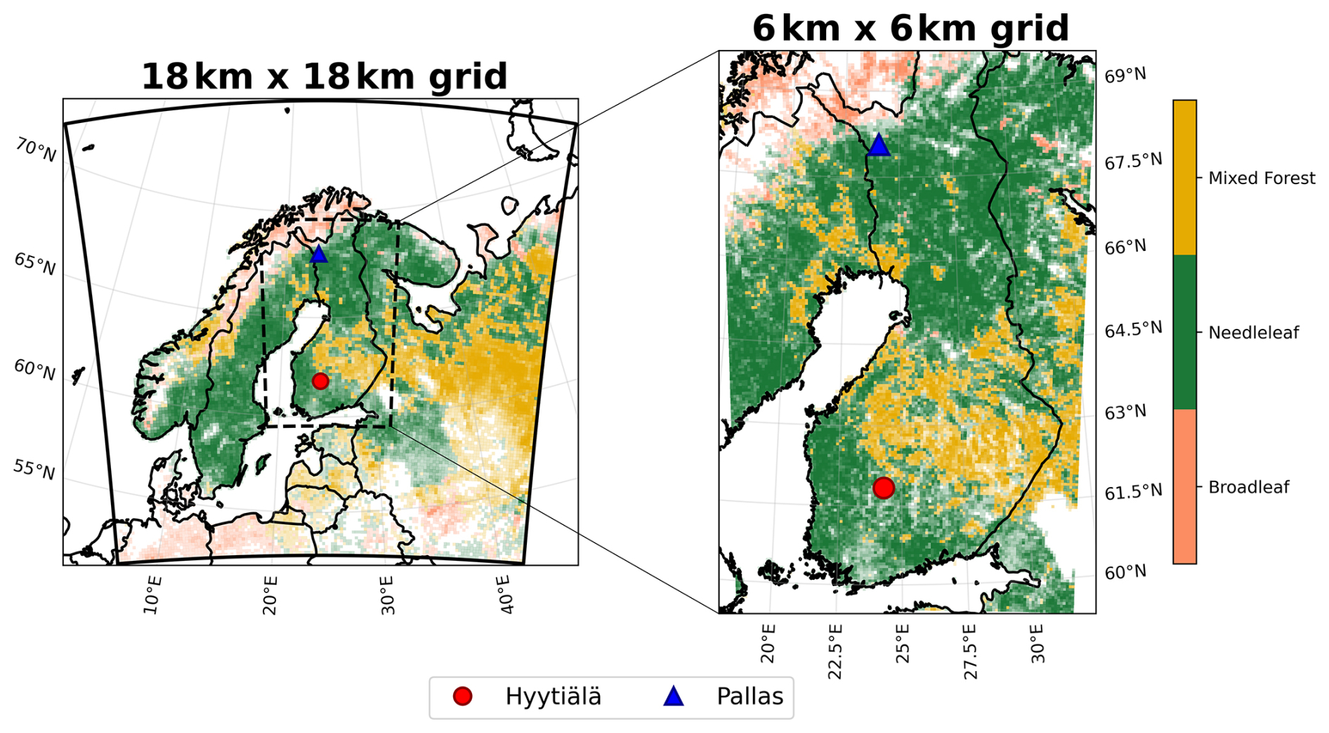
Figure 1 The two model domains: the parent domain with a grid cell size of 18 km×18 km, and the nested domain with a grid cell size of 6 km×6 km. The black line on the parent domain indicates the boundary of the domain, while the black dashed line indicates the position of the nested domain. The red circle denotes the location of the SMEAR-II station in Hyytiälä, while the blue triangle denotes the location of the Sammaltunturi station in Pallas. The color indicates the forest type in each grid cell, while the transparency represents the percentage of the cell covered by forest based on USGS land cover data.

2.1.1 Model input data

Meteorological inputs were generated using version 4.3 of the WRF model (Skamarock et al., 2019). The model was forced with reanalysis data from the National Centers for Environmental Prediction (NCEP) Climate Forecast System Version 2, at a temporal resolution of 6 h and a horizontal resolution of 1°, with the coarse domain nudged toward the reanalysis fields to maintain consistency.

Atmospheric composition boundary and initial conditions were retrieved from climatological simulations of LMDz-INCA3 (Hauglustaine et al., 2014) for gaseous and particulate species and GOCART (Chin et al., 2002) for dust concentrations.

Yearly anthropogenic emissions of carbon monoxide (CO), ammonia (NH₃), non-methane volatile organic compounds (NMVOCs), nitrogen oxides (NO_x), particulate matter (PM₁₀ and PM_2.5), and sulfur dioxide (SO₂) were retrieved by the CAMS-REG version 6.1 dataset (Kuenen et al., 2022) at a 0.05°×0.1° grid resolution. These emissions were distributed hourly across the study periods using temporal profiles derived from the EMEP MSC-W model (Simpson et al., 2012).

Biogenic emissions were calculated using the MEGANv2.1 algorithm, which is automatically integrated into the CHIMERE model. This version provides pre-calculated EFs for isoprene (C₅H₈), monoterpenes (divided in α-pinene, β-pinene, limonene, ocimene), humulene and β-caryophyllene with a horizontal resolution of 0.008°×0.008°. Additionally, sensitivity simulations were conducted in which the EFs for isoprene were recalculated using the more recent MEGANv3.2. Further details on this are provided in Sect. 2.3.

2.1.2 Sensitivity simulations

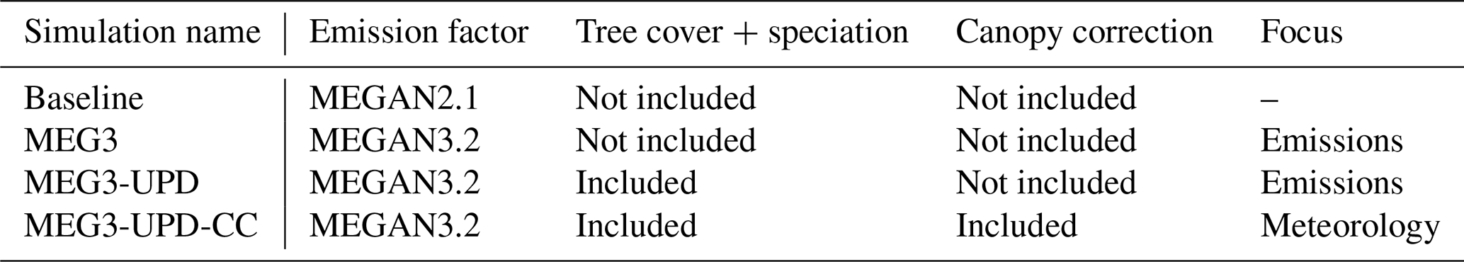
In addition to the baseline simulation, we conducted three sensitivity simulations aimed at improving the estimates of isoprene emissions and concentrations in the model. In the first sensitivity simulation, MEGANv3.2, without any additional modification of the inputs, was used to calculate the EFs for isoprene. The second sensitivity simulation introduced new isoprene EFs calculated with MEGANv3.2, incorporating domain-specific tree cover, tree species distribution, and species-specific EFs (more details are provided in Sect. 2.3). In the final sensitivity simulation built upon the second, we added a canopy correction to the first model layer, based on the approach introduced by Cholakian et al. (2023), to account for the effects of forest canopy on dispersion (further details are provided in the Supplement). This correction was required because WRF-CHIMERE does not explicitly represent canopy-induced effects on mixing and dispersion, which can lead to biases in simulated BVOC concentrations and their evaluation against observations. Table 1 summarizes the main characteristics of each simulation.

Table 1 Summary of the modification between each simulation. The “Emission factor” column refers to which version of MEGAN has been used to calculate the EF. The “Tree cover + speciation” column indicates whether updated tree cover and species distribution have been taken into account or not. The “Canopy correction” column shows which simulation includes the canopy correction. The “Focus” column highlights the main focus of each sensitivity simulation.

2.2 MEGAN emission model

BVOC emissions are estimated using the Model of Emissions of Gases and Aerosols from Nature (MEGAN; Guenther et al., 2006, 2020). Both MEGANv3.2 and MEGANv2.1 share the same general emission equation:

$$\begin{array}{}\text{(1)}& E=\text{EF}\cdot \text{EA}\end{array}$$

The two versions differ in both the definition of EF and the formulation of EA. In MEGANv3.2, the EA is defined as follows:

$$\begin{array}{ll}{\displaystyle }{\text{EA}}_{\text{v3.2}}=& {\displaystyle }\text{Cce}\cdot \text{LAI}\cdot {\mathit{\gamma }}_{\mathrm{P}}\cdot {\mathit{\gamma }}_{\mathrm{T}}\cdot {\mathit{\gamma }}_{\text{HT}}\cdot {\mathit{\gamma }}_{\text{LT}}\cdot {\mathit{\gamma }}_{\text{SW}}\cdot {\mathit{\gamma }}_{{\mathrm{O}}_{\mathrm{3}}}\\ \text{(2)}& {\displaystyle }& {\displaystyle }\cdot {\mathit{\gamma }}_{\mathrm{A}}\cdot {\mathit{\gamma }}_{\text{SM}}\cdot {\mathit{\gamma }}_{{\mathrm{CO}}_{\mathrm{2}}}\end{array}$$

where Cce represents the canopy environment coefficient accounting for within-canopy light and environmental attenuation, LAI is the leaf area index, γ_P, γ_T, γ_HT, γ_LT, γ_SW, ${\mathit{\gamma }}_{{\mathrm{O}}_{\mathrm{3}}}$, γ_A, γ_SM, and ${\mathit{\gamma }}_{{\mathrm{CO}}_{\mathrm{2}}}$ represent the activity factors for downward shortwave radiation, 2 m air temperature, high temperature, low temperature, strong wind, CO₂ pollution, leaf age, soil moisture, and CO₂ concentration, respectively. In the MEGANv2.1 version implemented within CHIMERE, the EA term is:

$$\begin{array}{}\text{(3)}& {\displaystyle }{\displaystyle }{\text{EA}}_{\text{v2.1}}={\mathit{\gamma }}_{\text{LAI}}\cdot {\mathit{\gamma }}_{\mathrm{P}}\cdot {\mathit{\gamma }}_{\mathrm{T}}\cdot {\mathit{\gamma }}_{\mathrm{A}}\cdot {\mathit{\gamma }}_{\text{SM}}\end{array}$$

where ${\mathit{\gamma }}_{\text{LAI}}=\mathrm{0.49}\text{LAI}/\sqrt{\mathrm{1}+\mathrm{0.2}{\text{LAI}}^{\mathrm{2}}}$.

Because EF in MEGANv3.2 is defined per unit LAI while in MEGANv2.1 it is not, the two EF datasets are not directly interchangeable. Equating Eqs. (2) and (3) at standard conditions and solving for EF_v2.1 gives:

$$\begin{array}{ll}{\displaystyle }{\text{EF}}_{\text{v2.1}}& {\displaystyle }={\text{EF}}_{\text{v3.2}}\cdot {\displaystyle \frac{\text{LAI}\cdot \text{Cce}}{{\mathit{\gamma }}_{\text{LAI}}}}\\ \text{(4)}& {\displaystyle }& {\displaystyle }={\text{EF}}_{\text{v3.2}}\cdot {\displaystyle \frac{\text{Cce}}{\mathrm{0.49}}}\cdot \sqrt{\mathrm{1}+\mathrm{0.2}\cdot {\text{LAI}}^{\mathrm{2}}}\end{array}$$

where LAI in Eq. (4) is at standard condition (i.e. 5 m² m⁻²).

2.3 Isoprene emission potential

To begin, we would like to clarify the terminology used throughout this text, as EF can refer to different concepts. When we use the general term EF, we refer specifically to the ecosystem level. To differentiate this from the EF associated with a specific tree species, we will consistently use the term “species-specific EF” when referring to the latter. Additionally, from here onwards, we use the term emission potential (EP) to refer to the “emission capacity” of the entire grid cell. The EP is used in the MEGANv2.1 algorithm to calculate actual emissions.

Since the MEGANv2.1 algorithm is already integrated into CHIMERE, here we use the MEGANv3.2 EF processor (MEGEFP) only to calculate updated EPs for isoprene. These updated EPs, based on domain-specific vegetation data, were then used as input for the MEGANv2.1 algorithm within CHIMERE. This means that, in this study, all the differences in the final emissions result from modifications to the EPs, not from changes in the activity-factor calculation.

The MEGEFP assigns distinct ecotypes to different regions. For each ecotype, specific tree species are assigned along with their species-specific EF and relative abundances. However, most ecotypes classify trees into two categories only: needleleaf and broadleaf. Although each ecotype includes an ecotype-specific needleleaf and broadleaf class, each with its own species-specific EF, this approach is not fully representative of reality. For example, Picea abies (Norway spruce) has a species-specific isoprene EF at least one order of magnitude larger than that of Pinus sylvestris (Scots pine) (Lindfors and Laurila, 2000; Tarvainen et al., 2005; Hakola et al., 2023), despite both being classified as needleleaf trees and found in boreal forests.

To improve the accuracy of the EPs, we retrieved high-resolution data on tree cover, tree species distribution, and tree species-specific EF tailored to Finland. This data was then used to update the MEGEFP inputs, allowing for more regionally representative calculations of isoprene emissions. Specifically, this process consists of three main steps (a schematic is shown in Fig. 2). In the first step, tree cover data for the year 2019 were retrieved from the Natural Resources Institute Finland (LUKE) website (https://kartta.luke.fi, last access: 20 January 2026) and updated into MEGEFP. During the second step, we retrieved from the same website information about the spatial distribution of three main tree species present in Finland (Scots pine, Norway spruce, and Silver birch), which together account for 97 % of all trees. To implement these data in MEGEFP, we utilized its functionality that allows for the definition of multiple ecotypes within the same grid cell, along with the assignment of the percentage of the grid cell covered by each ecotype. Accordingly, we defined three new mono-species ecotypes and assigned the relative percentage of each ecotype based on the retrieved data. This method allows us to include the spatial distribution information for the different tree species in the model, with a high spatial resolution. An alternative, simpler implementation of the second step was also tested. In this version, the original ecotype spatial distribution was retained, and we assumed a uniform distribution of 50 % Scots pine, 30 % Norway spruce, and 20 % Silver birch across the entire ecotype. These percentages represent roughly the average tree species abundance in Finland. This “simple” version was compared to the previous “advanced” version only in terms of the final EPs grid and was not used as input for emissions calculation within CHIMERE. This simplified version was tested because detailed information on tree species distribution is often unavailable in many regions around the world. In such cases, step 2 cannot be implemented, making an alternative approach necessary. Comparing the simplified and advanced versions allows us to quantify the differences, and thus the uncertainties, introduced by assuming a uniform species distribution. In the final step, species-specific isoprene EFs for Scots pine, Norway spruce, and Silver Birch were retrieved from the literature (Lindfors and Laurila, 2000; Tarvainen et al., 2005; Hakola et al., 2023) and incorporated into the EFs tables of MEGEFP. Specifically, for Norway spruce, we used the median value of all the EFs available, while for Scots pine and Silver birch, we assigned the minimum value present in MEGANv3.2, as for both species, extremely small EFs are reported in Finland (Lindfors and Laurila, 2000). It is important to acknowledge that for Norway spruce, reported isoprene EFs span a very wide range (0–7140 $\mathrm{ng}{\mathrm{g}}_{\left(\mathrm{dw}\right)}^{-\mathrm{1}}{\mathrm{h}}^{-\mathrm{1}}$), introducing a notable source of uncertainty. This variability reflects differences in measurement approaches, environmental conditions, and site-specific factors, and represents a limitation in the current emission estimates. Consequently, the choice of a representative value (e.g. median) may influence the resulting emissions. We can quantify the uncertainty introduced by this choice by evaluating the interquartile range of reported values, which yields an estimated uncertainty of approximately −85 % to +370 % relative to the median. However, the full literature range represents an extreme upper-bound uncertainty that is unlikely to be representative at the ecosystem scale, where spatial averaging across many trees and environmental conditions is expected to reduce the influence of extreme individual measurements.

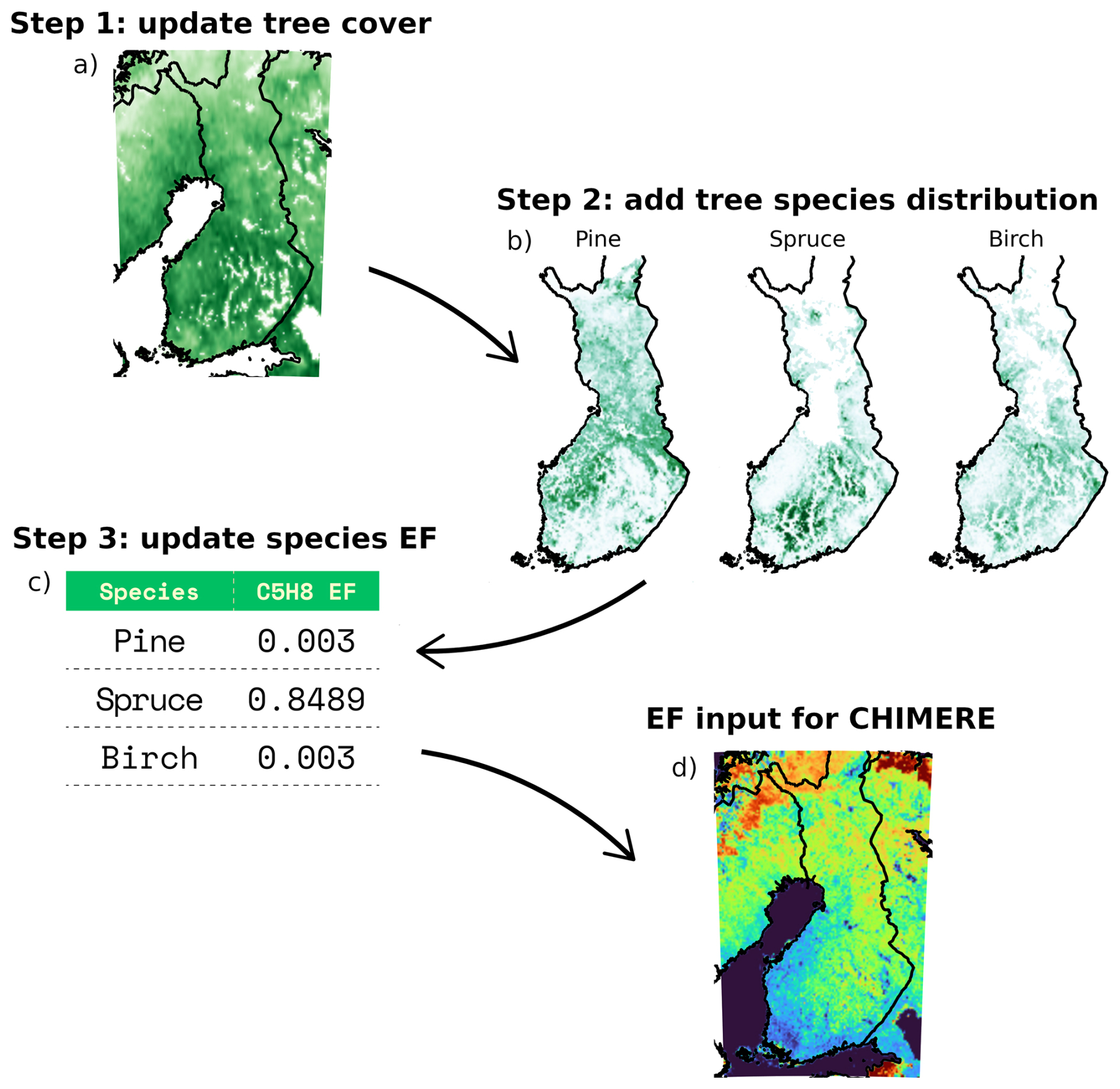
Figure 2 Schematic of the isoprene EP calculation. The scheme shows only the input to the MEGAN3 EF processor that has been modified in this study. These modifications include updating the tree cover percentage (a), the tree species distribution (b), and the species-specific emission factors for isoprene (in units of nanomoles ${\mathrm{m}}^{-\mathrm{2}}{\mathrm{s}}^{-\mathrm{1}}{\mathrm{LAI}}^{-\mathrm{1}}$) (c). The final output is the gridded isoprene EP (d), which can be used as input for the MEGAN version integrated within the CHIMERE model.

2.4 FLEXPART

The FLEXible PARTicle dispersion model (FLEXPART) is a Lagrangian model used to simulate both the forward and backward dispersion of particles. In this study, we used WRF-FLEXPART version 3.3.2 (Brioude et al., 2013) in backward mode to trace air-mass origins arriving at Hyytiälä. Simulations were driven by meteorological data generated from the WRF simulations (the same used for the CHIMERE simulations), with a temporal resolution of 20 min.

The FLEXPART model was configured with one domain matching the resolution and region covered by the outermost domain of the WRF-CHIMERE simulations, with a resolution of 18 km×18 km. This domain was designed to capture long-range transport processes. The simulation was set up with 12 vertical levels extending from the surface to 9000 $\mathrm{m}\mathrm{a}.\mathrm{g}.\mathrm{l}.$ The layer thickness follows a pseudo-exponential distribution, with finer resolution (50 m) near the surface and progressively increasing layer depth with altitude.

During the study period, we released 10 000 particles per hour from Hyytiälä and tracked their back trajectories over 72 h. The passive tracer particles were emitted from altitudes ranging from 0 to 100 $\mathrm{m}\mathrm{a}.\mathrm{g}.\mathrm{l}.$ The output of FLEXPART in backward mode is the Source–Receptor Relationship (SRR), expressed in units of seconds, representing the residence time of particles in each grid cell, i.e. the time spent by particles released at the receptor in a given grid cell during the backward simulation.

To investigate the impact of air mass history on measured and modelled OA concentrations at Hyytiälä, and to better understand potential sources of bias, we combined OA time series from Hyytiälä with FLEXPART output. Specifically, we calculated the Source Region Contribution (SRC) as described in Bettineschi et al. (2025). Given a simulation domain Ω, defined as the four-dimensional spatiotemporal domain of the FLEXPART simulation including time (t), height (h), longitude (x), and latitude (y) over the 72 h back-trajectory, and an air mass arrival time (τ), defined as the time of particle release at the receptor (i.e. the measurement time at Hyytiälä), the SRC was calculated assigning the OA concentration/bias recorded during τ, to all the (x,y) grid points intercepted by the air mass (at any height) in the 72 h prior the release and doing a sum over all the releases, then for each (x,y) pair this value is divided by the number of trajectories that have been intercepted by the given (x,y) grid point. This can be mathematically described by the following equations:

$$\begin{array}{}\text{(5)}& {\displaystyle }& {\displaystyle }\text{SRC}(x,y)={\displaystyle \frac{{\sum }_{\mathit{\tau }}\mathit{\delta }(\mathit{\tau };x,y)\cdot \left[\text{OA}\right]\left(\mathit{\tau }\right)}{{\sum }_{\mathit{\tau }}\mathit{\delta }(\mathit{\tau };x,y)}}\text{(6)}& {\displaystyle }& {\displaystyle }\mathit{\delta }(x,y,\mathit{\tau })=\left\{\begin{array}{ll}\mathrm{1}& \text{if }\sum _{(t,h)\in \mathrm{\Omega }}\text{SRR}(t,h;x,y,\mathit{\tau })>\mathrm{0}\\ \mathrm{0}& \text{otherwise}\end{array}\right.\end{array}$$

The SRC metric in this study was used to compare the source regions of measured OA vs. modelled OA. This can provide information on whether the model has a stronger bias when air masses arrive from a specific region, or if the bias is independent of air mass origin. The SRC formulation does not explicitly account for the chemical lifetime of OA, and it is used here as a source-region diagnostic rather than a quantitative source apportionment tool.

Additionally, to further understand the relationship between air masses and OA, we adapted the concept of Air Mass Exposure (AME), as introduced by Hakala et al. (2022). AME calculations combine FLEXPART output with two-dimensional fields (e.g. emissions fields or population density) to determine when air masses were exposed to emissions from different pollutants. Here, we modified the AME calculation by integrating the FLEXPART output with the three-dimensional emissions (i.e. including also the time dimensions) calculated by MEGAN. For each release event, we calculated the AME to monoterpenes emissions according to the following equation:

$$\begin{array}{ll}{\displaystyle }\text{AME}\left(\mathit{\tau }\right)=\sum _{(t,x,y)\in \mathrm{\Omega }}& {\displaystyle }{\text{SRR}}_{\mathrm{500}}(t,x,y;\mathit{\tau })\\ \text{(7)}& {\displaystyle }& {\displaystyle }\cdot \left[\text{Monoterpenes}\right](t,x,y)\text{(8)}& {\displaystyle }{\text{SRR}}_{\mathrm{500}}(t,x,y,\mathit{\tau })=& {\displaystyle }\sum _{h=\mathrm{0}}^{\mathrm{500}\mathrm{m}}\text{SRR}(h;t,x,y,\mathit{\tau })\end{array}$$

It is important to highlight that using a fixed integration depth could potentially bias the AME metric. However, integrating over a fixed vertical depth is a standard approach used in many other studies (Aliaga et al., 2021; Hakala et al., 2022; Bettineschi et al., 2025). The reason is that it provides a framework independent of uncertainties in planetary boundary layer height estimation, which can vary substantially across models and calculation methods. Using a fixed depth avoids introducing additional variability and potential errors associated with diagnosing PBLH. Furthermore, Bettineschi et al. (2025) showed that using a fixed depth or a depth that varies with the PBLH (simulated by WRF) does not result in substantial differences in the resulting metrics, suggesting that the sensitivity of AME to the choice of integration depth is limited.

2.5 Observational data

A diverse set of observational data was used to evaluate the different simulations. Temperature and wind speed measurements from Hyytiälä (see Fig. 1) were obtained from the https://smear.avaa.csc.fi website (last access: 20 January 2026) (Junninen et al., 2009) for the entire simulation period. These observations are available at various heights, and in this study, we used all data available within the 2–125 m range.

Ecosystem level BVOCs fluxes from Hyytiälä are used in this study to evaluate the simulated emissions. The BVOC fluxes used here are measured using the surface-layer-profile method with a proton transfer reaction mass spectrometer (PTR-MS) (Rantala et al., 2014), the systematic error of this technique is estimated to be around 10 %.

Ground level BVOCs concentrations from Hyytiälä were also retrieved from the https://smear.avaa.csc.fi website (Junninen et al., 2009). Additionally, isoprene concentration from Pallas (see Fig. 1) at ground level was retrieved from the EBAS website (https://ebas.nilu.no, last access: 20 January 2026).

OA concentrations from Hyytiälä are measured with an Aerosol Chemical Speciation Monitor (ACSM), as described by Heikkinen et al. (2020).

3 Results

3.1 Meteorological evaluation

Meteorological conditions play a fundamental role in the simulation of BVOCs emissions and the following aerosol formations and transportation processes. It is thus important to assess whether the main meteorological variables are simulated correctly or not. Figure 3 reports an evaluation of the model performance in relation to temperature and wind speed. The comparison of the vertical profile of average temperature (Fig. 3a) shows that the model is in good agreement with the observations, with a small constant underestimation at all heights between 4–125 $\mathrm{m}\mathrm{a}.\mathrm{g}.\mathrm{l}.$ Similarly, the 2 m hourly temperature (Fig. 3c) is in good agreement across the whole temperature range recorded, which spans roughly 30 °C, despite a mean underestimation of 0.74 °C in the model. This underestimation occurs mainly during nighttime hours, as shown in the diurnal cycle reported in the Supplement (Fig. S1). Similar cold biases during nighttime have been reported before in several studies (Holtslag et al., 2013; García-Díez et al., 2013; Ciarelli et al., 2024), and it is thought to be caused by excessive vertical mixing in the model during stable boundary layer conditions.

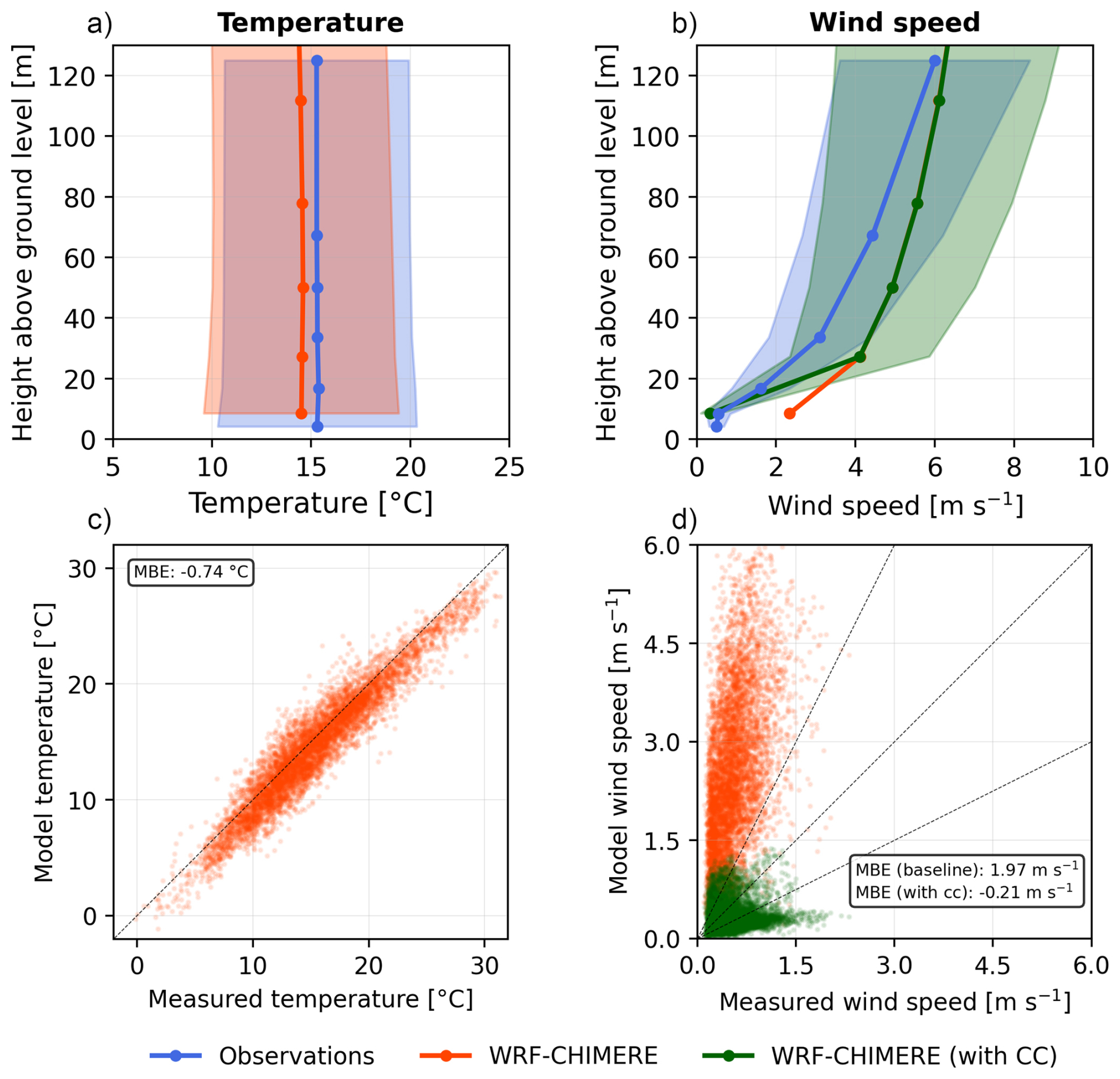
Figure 3 Vertical profiles of mean temperature (a) and wind speed (b), comparing observations at Hyytiälä, and the nearest grid point in the WRF-CHIMERE simulation. In (b), we also show the WRF-CHIMERE simulation with canopy correction (CC). The dots indicate the height of the measurements or the mid-layer height. The shaded area represents the standard deviation from the mean, not reported for the baseline simulation in (b), for better readability of the plot. Comparison of the measured and modelled 2 m temperature (c), and wind speed at 8 m (d). Panel (d) shows the baseline (orange) and canopy correction (green) simulations.

As shown in Fig. 3b, the wind speed vertical profiles indicate a strong bias compared to the observations. Specifically, in the baseline simulation, the closer to the ground the bigger the overestimation in the model. This is caused by the absence of a coupled canopy model in CHIMERE, which means it cannot take into account the physical effect of the forest canopy on wind speed. We tested the effect of adding a simple canopy correction acting on the first layer of the model as described in the Supplement. Figure 3b and d show that the canopy correction significantly improves the performance in the first layer of the model, with the mean bias error (MBE) going from 1.97 m s⁻¹ in the baseline simulation to −0.21 m s⁻¹ in the simulation with the canopy correction.

3.2 Isoprene emission potential

The effects of using different input datasets on the calculation of EPs are presented in this section. Figure 4 shows the individual impact of each modification on isoprene EPs across Finland, compared to the baseline MEGANv3.2 configuration.

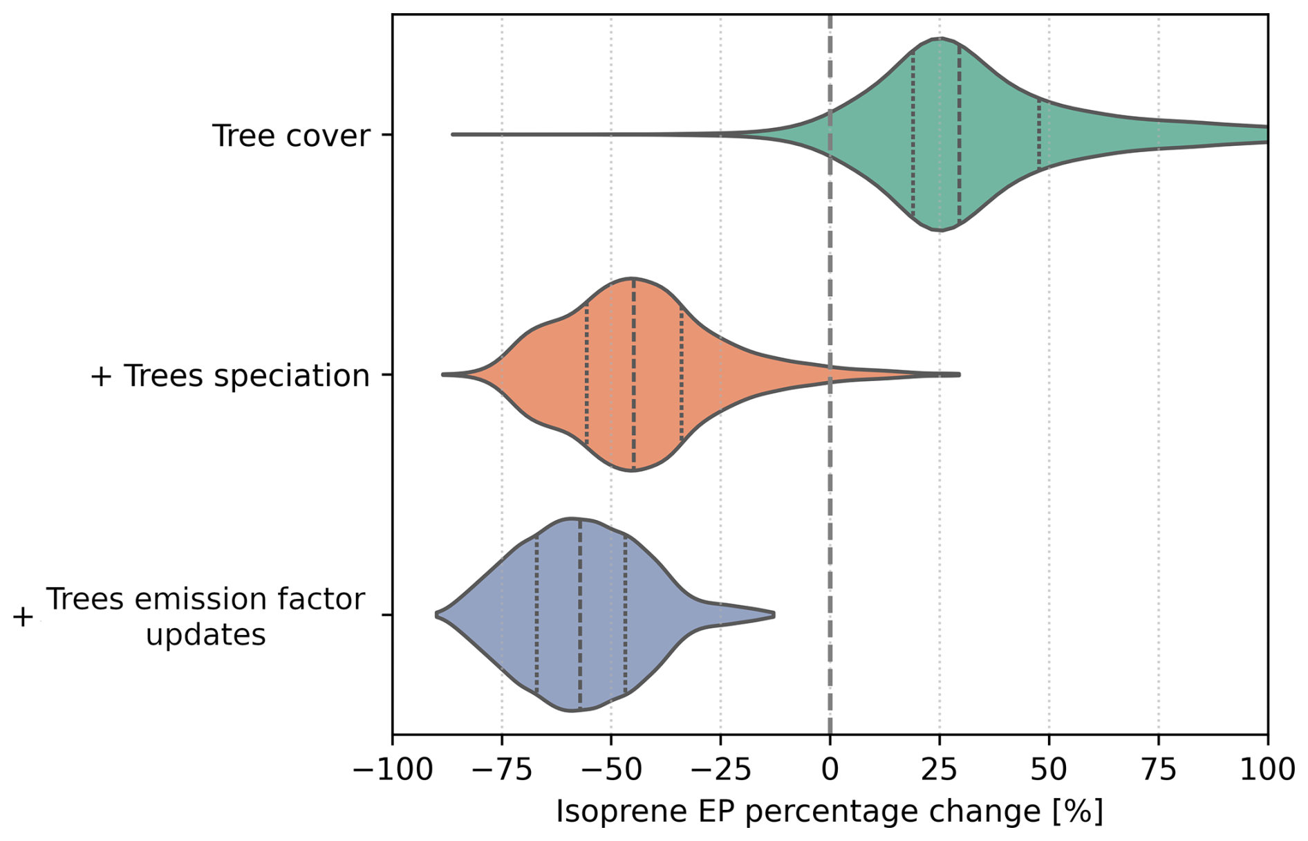
Figure 4 Violin plots of the isoprene emission factor percentage change for the different input modifications. The variation is calculated over the whole of Finland in comparison to the base MEGANv3.2 emission factor. The + indicates that the modification is added on top of the previous one. The three modifications correspond to the three steps shown in Fig. 2. The vertical dotted line inside the violin plot represents the interquartile range and the median value.

Updating the tree cover distribution using high-resolution LUKE data results in a general increase in isoprene EPs across most of Finland. In the majority of grid cells, this increase exceeds 25 %. Assuming the LUKE dataset represents the ground truth, this suggests that the tree cover data used in the base MEGANv3.2 version is likely incorrect for Finland and underestimates the actual tree cover.

Adding tree species distribution information on top of the LUKE tree cover leads to a significant decrease in isoprene EPs. This reduction is primarily due to the higher accuracy of the species-specific EFs already present in MEGANv3.2 for Norway spruce, Scots pine, and Silver birch, compared to the more generic species-specific EFs used for the needleleaf/broadleaf “species”. This trend continues with the final modification, where only the species-specific EFs are updated. While isoprene EPs still decrease, the variation is smaller than in the previous step. This is because the original species-specific isoprene EFs used in MEGANv3.2 are already reasonably accurate.

Adding information about species distribution (i.e. step 2) not only changes the absolute values of the EPs (which could have also been achieved by simply modifying the species-specific isoprene EFs assigned to the needleleaf/broadleaf “species”), but also significantly changes their spatial distribution. This is illustrated in Fig. 5, which compares two different approaches used in step 2. Assuming a uniform species distribution (“simple” speciation) results in a relative difference in isoprene EPs ranging approximately from −20 % to +20 %, compared to using a more detailed species distribution (“advanced” speciation). These differences are primarily driven by the distribution of Norway Spruce (see Fig. 2), the main isoprene emitter in Finland. In regions with a high relative abundance of Norway spruce, the “simple” speciation approach underestimates isoprene EPs (as shown by the blue areas in Fig. 5). The opposite occurs in areas where Scots pine dominates, leading to an overestimation of EPs using the simplified approach.

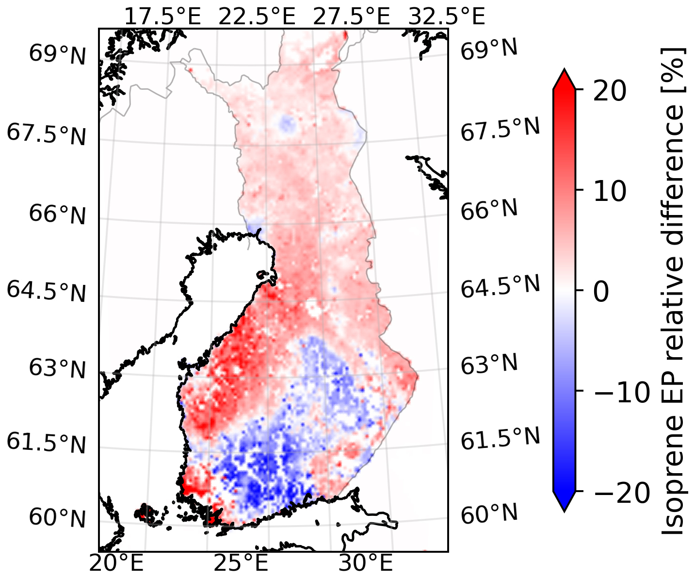
Figure 5 Relative difference between the isoprene emission factors calculated using the “simple” speciation compared to the “advanced” speciation. The “advanced” EPs have been used as a reference.

3.3 Isoprene emission

The effects of using the new isoprene EPs, including all the updated inputs, on modelled isoprene emissions are presented in this section. Figure 6a compares the observed average diurnal cycle of isoprene emissions during summer at the Hyytiälä site with modelled isoprene diurnal emissions from three simulations, each using a different set of EPs. The baseline simulation, which uses the pre-calculated EPs from MEGANv2.1, greatly overestimates isoprene emissions, consistent with previous findings (Jiang et al., 2019; Cholakian et al., 2023; Zhao et al., 2024; Ciarelli et al., 2024). The MEG3 simulation (see Table 1), which uses EPs calculated with the default version of MEGANv3.2, reduces this overestimation by roughly a factor of two. However, despite this improvement, the emissions remain overestimated. The MEG3-UPD simulation, which uses EPs calculated with MEGANv3.2 incorporating all the updated inputs, shows the best performance, with modelled emissions closely matching observations, despite a slight underestimation.

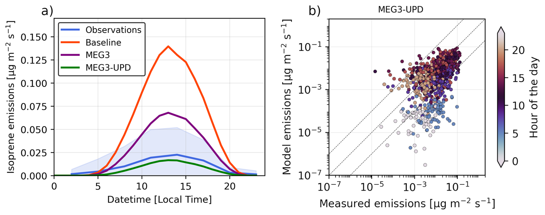
Figure 6 (a) Diurnal variation of observed and WRF-CHIMERE modelled isoprene emissions at Hyytiälä. The mean (solid lines) is reported for observations and all the simulations with different emissions, while the standard deviation (shaded area) is reported only for the observations for better visibility. (b) Scatter plot comparing measured and model-predicted hourly isoprene emissions in log scale. Only the MEG3-UPD simulation is shown. The MBE is displayed in the upper left corner. The dashed lines represent the 10:1, 1:1, and 1:10 agreement between observations and model predictions.

Figure 6b provides a more detailed comparison between the observations and the final simulation. The vast majority of hourly data (79 %) fall within an order of magnitude of the observations. A cluster of points, however, shows underestimations greater than a factor of ten; these correspond mostly to nighttime (when in Hyytiälä light levels during short summer nights allow low but non-zero isoprene emissions). Possible explanations include: (i) the underestimation may be driven by a bias in the simulated diurnal temperature cycle. As mentioned earlier, the model underestimates temperature during night, which could lead to lower simulated isoprene emissions; (ii) the bias could arise from the measurements technique, as during night some isoprene emitted the day before is trapped inside the canopy, during sunrise (in Hyytiälä during summer as early as 03:00 a.m. LT) with the development of the boundary layer some of this isoprene can be transported upwards and detected as a flux. In other words, since the observations measure ecosystem-level fluxes, the direct comparison with emissions might not always be possible. However, if this explanation is correct, it accounts only for a subset of the underestimated points, namely the blue points, which correspond roughly to the sunrise hours.

In Fig. 7, the spatial distribution of isoprene emissions from the MEG3-UPD simulation is compared with those from the CAMS-GLOB-BIOv3.1 (CAMS-BIO hereafter) dataset, which has a spatial resolution of 0.25°×0.25°, and also uses MEGANv2.1 (Sindelarova et al., 2022). This dataset is widely used for global and regional modelling and also includes updated isoprene emissions over Europe. Overall, the two datasets show the same order of magnitude over many areas. The largest differences arise in the spatial patterns: CAMS-BIO shows higher emissions in southwestern Finland and in some areas of Lapland compared to MEG3-UPD. Furthermore, the CAMS-BIO dataset does not capture the high-emission area associated with the high abundance of Norway Spruce, and it underestimates emissions in most of the domain.

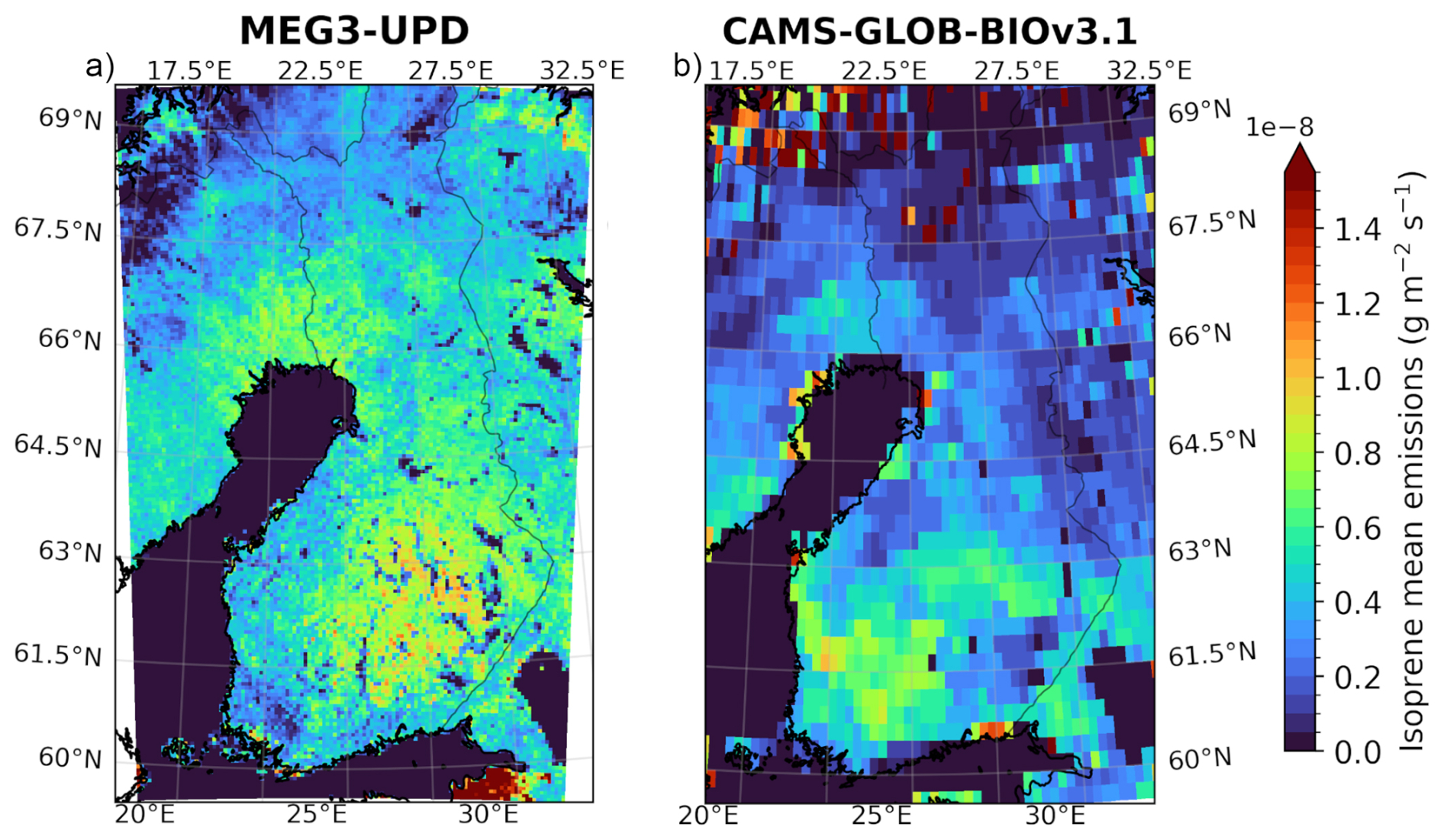
Figure 7 Comparison between the updated isoprene emission used in this study (a) and the CAMS-GLOB-BIOv3.1 dataset (b). Both represent only summer emissions during 2017, 2018, and 2019.

3.4 BVOCs concentrations

This section presents the evaluation of all simulations with respect to BVOCs concentrations. Specifically, for each simulation, we compared concentrations of isoprene, monoterpenes, methanol, and acetone with observations from Hyytiälä. In addition, isoprene concentrations were also compared with observations from Pallas.

As shown in Fig. 8a–d, in Hyytiälä the comparison of isoprene concentrations follows a pattern similar to the emissions, as expected: concentrations are greatly overestimated in the baseline simulation, improved by roughly a factor of two in the MEG3 simulation, and further reduced in the MEG3-UPD simulation. Interestingly, the MEG3 simulation yields the lowest MBE across all simulations. We attribute this to a double bias compensation, where excessive emissions cause overestimation, while the absence of a canopy correction leads to underestimation. This interpretation is supported by the MEG3-UPD-CC results (panel d), which show that including a canopy correction increases isoprene concentrations at ground level. Similar results are found at Pallas (Fig. 9), although in this case the MEG3-UPD simulation has the lowest MBE, closely followed by MEG3-UPD-CC. This confirms the good performance of the updated emissions when compared to an environment (tundra) that is significantly different from the Hyytiälä pine forest. Additionally, in Pallas, the canopy correction has a smaller effect compared to Hyytiälä, as Pallas is not located inside a forest canopy.

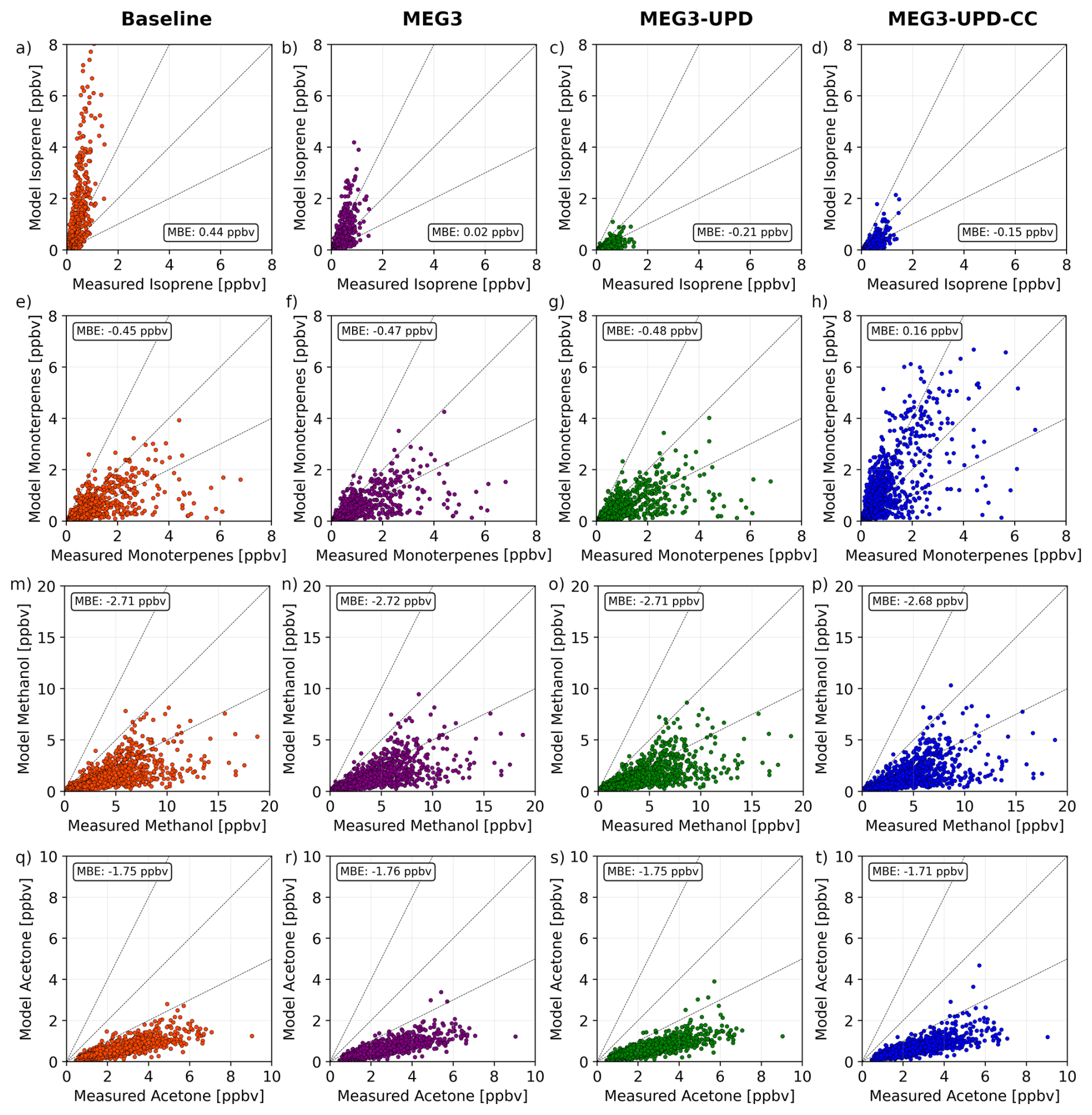
Figure 8 Scatter plot comparing measured and model-predicted concentrations for isoprene (a–d), monoterpenes (e–h), methanol (m–p), and acetone (q–t) at Hyytiälä, under the baseline simulation and all sensitivity simulations (MEG3, MEG3-UPD, and MEG3-UPD-CC). Each panel represents a specific combination of compound and simulation, with the MBE indicated in the corner of each subplot. The dashed lines represent the 2:1, 1:1, and 1:2 agreements between observations and model predictions.

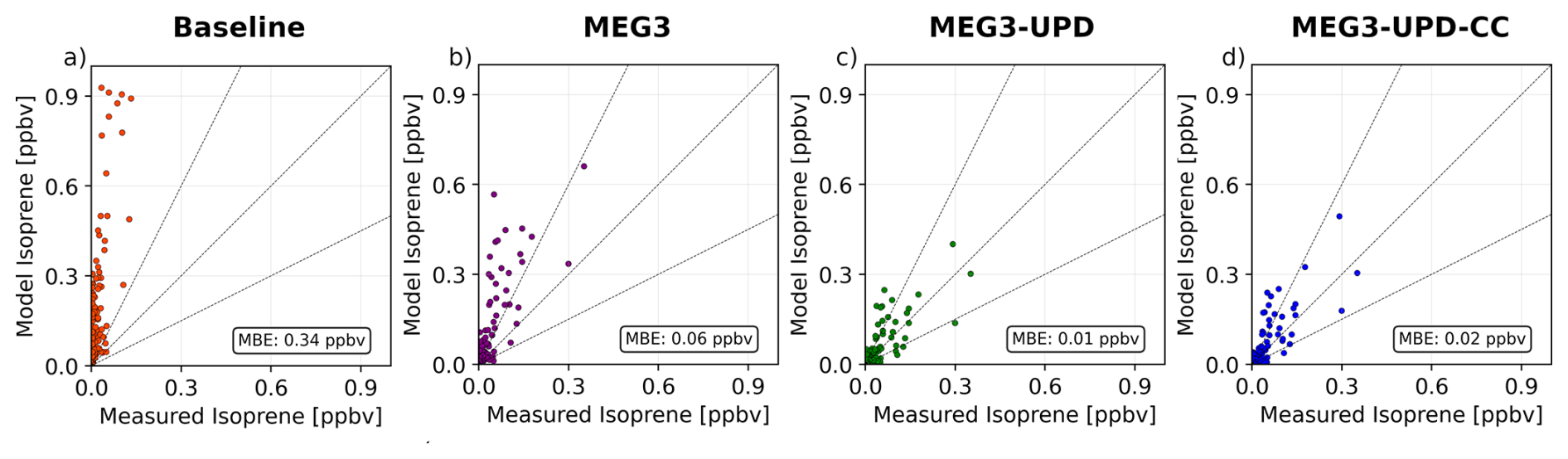
Figure 9 Scatter plot comparing measured and model-predicted concentrations for isoprene at the Pallas station under the baseline simulation and all sensitivity simulations (MEG3, MEG3-UPD, and MEG3-UPD-CC). The MBE is indicated in the corner of each subplot. The dashed lines represent the 2:1, 1:1, and 1:2 agreements between observations and model predictions.

Figure 8e–h presents the same comparison for monoterpenes. Although monoterpenes emissions were not modified, it is interesting to note that monoterpenes concentrations decrease slightly as isoprene decreases. While the effect is very small, this is consistent with the understanding that isoprene can effectively scavenge OH radicals, reducing their availability to react with monoterpenes. As a consequence, lower isoprene levels translate into more OH available for monoterpenes oxidation, resulting in a higher monoterpenes sink. The results also show that the canopy correction has a notable influence on monoterpenes concentrations, similar to its effect on isoprene. Overall, monoterpenes concentrations are more scattered than those of the other BVOCs, suggesting greater complexity in monoterpenes modelling.

Figure 8m–t shows the same comparison for methanol and acetone. Similar to monoterpenes, emissions of these compounds were not modified, resulting in only very small predicted changes across the simulations with only isoprene emissions modified. Interestingly, for both methanol and acetone, the canopy correction has a much smaller effect compared to its impact on isoprene or monoterpenes. This is likely because methanol and acetone have significantly longer atmospheric lifetimes than isoprene or monoterpenes. As a result, they are more evenly mixed in the atmosphere and more influenced by regional transport rather than local transport processes. Additionally, although the MBE for methanol and acetone is larger than for monoterpenes, the data points are less scattered. This suggests that emissions of methanol and acetone are likely underestimated, but their atmospheric behavior is simpler to model. A part of this under-prediction of emissions can be due to missing forest floor emissions as well as missing wetlands emissions, as both have been shown to be a significant source of methanol and acetone in the boreal region (Holst et al., 2010; Mäki et al., 2019).

3.5 Canopy correction effect on vertical transport of BVOCs

In this section, we analyze in more detail the effects of the canopy correction on the vertical transport of isoprene and monoterpenes by comparing the MEG3-UPD and the MEG3-UPD-CC simulations. Figure 10a–d shows that the impact of the canopy correction depends both on time of day and compound considered.

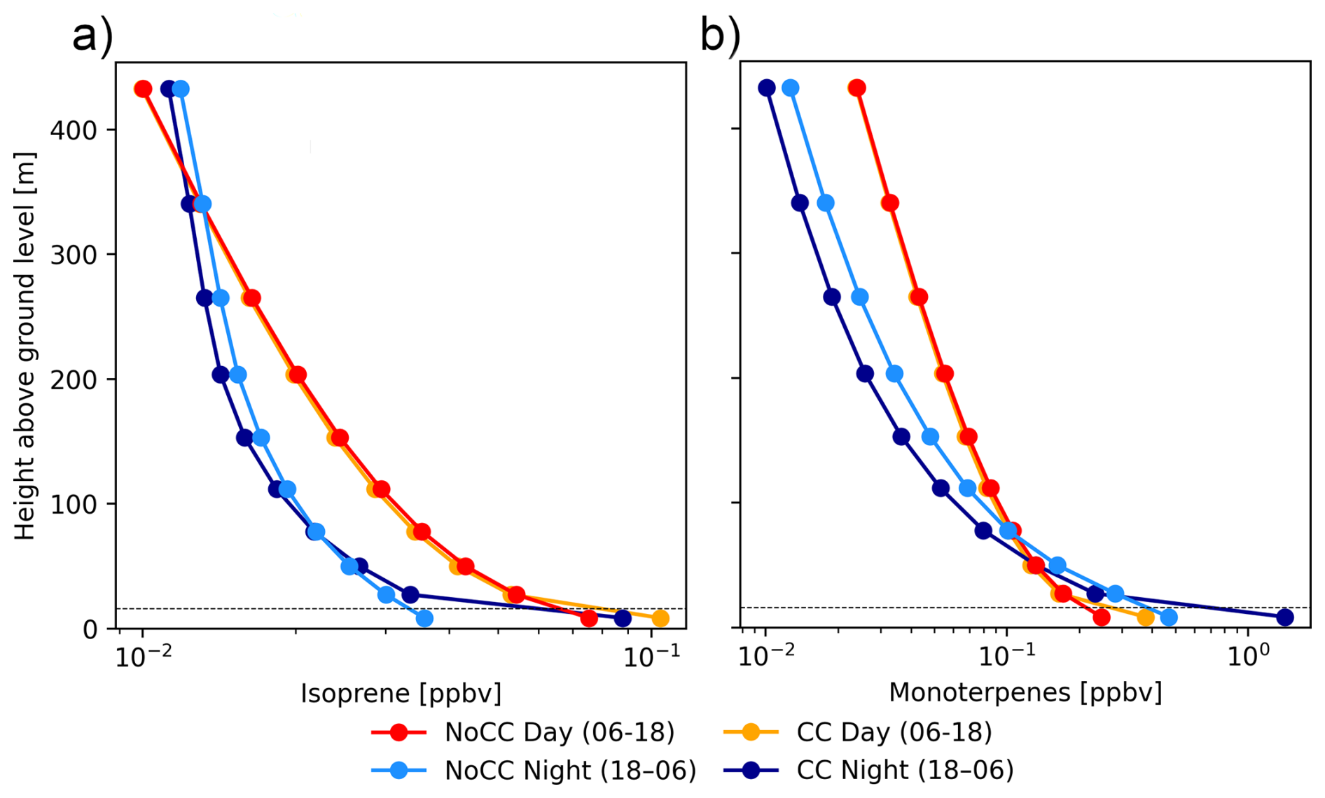
Figure 10 Average vertical profiles of isoprene (a) and monoterpenes (b) during the daytime (06:00–18:00 LT) and nighttime (18:00–06:00 LT). The horizontal dashed line represents the average canopy height in Hyytiälä. Only the first ten layers of the model are shown.

Overall, the canopy correction has the largest effect during nighttime. For both isoprene and monoterpenes, canopy correction leads to substantially higher concentrations inside the canopy at night compared to the MEG3-UPD simulation. For monoterpenes, this is the result of the nighttime emissions, which accumulate inside the forest canopy more efficiently than without canopy correction; this can be seen by looking at the difference between in-canopy concentrations during daytime and nighttime, with and without the canopy correction. For isoprene, this is just the result of the lower dispersion, as isoprene emissions are virtually zero during nighttime. This can be seen by the fact that during nighttime the concentrations are lower than during daytime. During daytime, however, the canopy correction effect is limited to within the canopy, while concentrations above the canopy remain largely unaffected; this suggests that during daytime, other processes (e.g. oxidation) have a stronger effect on concentrations above the canopy than vertical transport. Above the canopy, the canopy correction generally causes a slight decrease in nighttime concentrations. For monoterpenes, this reduction is visible immediately above the canopy, whereas for isoprene, it only becomes apparent above 80 m. However, the magnitude of this effect is extremely small.

3.6 Organic Aerosol

This section evaluates the OA concentrations simulated by WRF-CHIMERE, highlighting the effects of isoprene emission reductions and canopy correction. We also present the identification of potential sources of bias.

Figure 11 shows the comparison of observations in Hyytiälä against the baseline simulation (panel a) and the MEG3-UPD-CC simulation (panel b). The simulation that showed the best overall score when considering both isoprene emissions and concentrations (MEG3-UPD-CC) slightly reduced the OA bias when compared to the baseline simulation; however, both simulations show a similar pattern with a higher relative underestimation at low OA concentrations, while at higher concentrations the relative error is smaller. This suggests a possible underestimation of the background concentration, as this would have a bigger relative impact on periods with low concentrations. This missing background is likely due to either missing emissions or too low lateral boundary conditions. From the observations, we estimate the background concentration to be approximately 0.2 µg m⁻³. This indicates that the missing background can account for only a minor fraction of the model underestimation, particularly at high concentrations. To better identify the sources of bias in the modelled OA, we combined the hourly OA bias (OA_measured−OA_model) with air-mass back trajectories calculated using FLEXPART. Specifically, by applying the SRC metric, we assessed whether air masses traveling over certain regions are systematically associated with stronger OA underestimation.

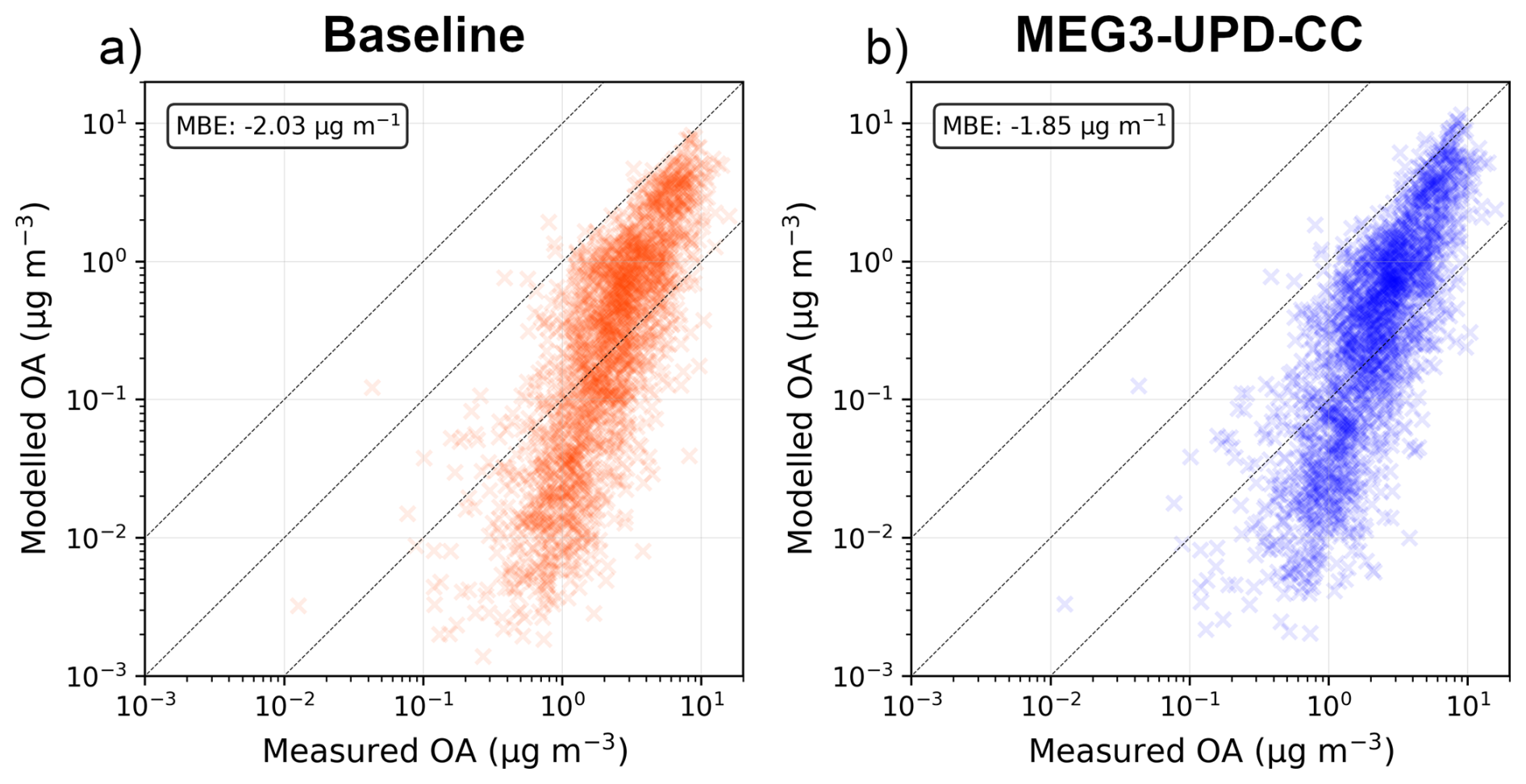
Figure 11 Comparison of OA observations at the Hyytiälä station with modelled OA from the baseline simulation (a) and the MEG3-UPD-CC simulation (b). The MBE for both simulations is indicated in the top-left corner.

Figure 12a presents the SRC to OA observations, showing that during summer, the highest OA concentrations occur when air masses arrive from the south. This finding is consistent with previous studies regarding Hyytiälä, which also identified southerly air masses as more polluted (Riuttanen et al., 2013; Petäjä et al., 2022). Similarly, Fig. 12b shows the SRC to OA bias, revealing that the strongest underestimation is linked to air masses arriving from the south and from the east. This suggests that the bias could be due to insufficient OA contributions from the southern and eastern boundary conditions of the model domain. Such underestimation could be mitigated either by artificially increasing the boundary concentrations or by expanding the domain size (assuming emissions are accurately represented). To verify this, a sensitivity simulation was conducted in which the first domain was expanded to cover the whole of Europe, as shown in Fig. S2. Due to computational and storage limit this simulation was performed only for the three summer months of 2018 (the year showing the largest bias). The results revealed only a marginal improvement in model performance, as shown in Fig. S3, suggesting that the configuration of the first domain accounts for only a minor portion of the overall bias, and it influences the bias only during specific time periods.

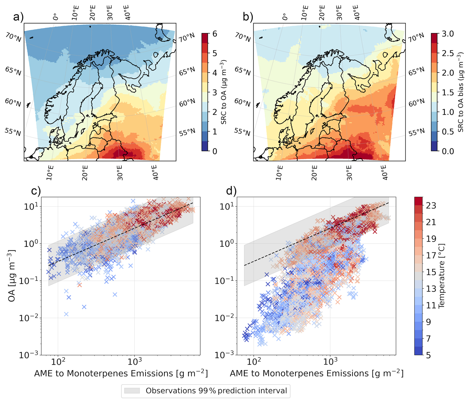
Figure 12 (a) Source region of the OA observed at the Hyytiälä station. The SRC was calculated by assigning the OA concentration measured during the release to all the grid cells intercepted by at least one particle in the 72 h prior to the release. (b) SRC to OA bias (${\text{OA}}_{\text{bias}}={\text{OA}}_{\text{measured}}-{\text{OA}}_{\text{model}}$). Note the difference in the color-bar scale. AME to monoterpenes emissions vs. measured OA (c) and modelled OA (d). In both (c) and (d), the 99 % prediction interval calculated on observations is shown.

As shown in Fig. 12c and d, the AME to monoterpene emissions appears to be another factor influencing the model bias. In general, variations in AME explain most of the variability in observed OA (R²=0.64). While this is also true for the modelled OA, where variation in the AME explains 62 % of the variability (R²=0.62), the modelled OA remains consistently lower than the observed OA across all AME levels. This suggests that the BSOA production in the model is under-predicted.

Another potential source of bias is the absence of forest fire emissions in our simulations. Forest fires release substantial amounts of OA and its precursors, which can be transported over long distances. As a result, forest fires can significantly contribute to OA concentrations even in regions far from the fire sources (Ortiz-Amezcua et al., 2017; He et al., 2024; Lee et al., 2025; Olonimoyo et al., 2026). Neglecting these emissions could therefore lead to an underestimation of background OA levels and partially explain the observed discrepancies.

The effects on the modelled OA concentrations of reducing isoprene emissions and adding the canopy correction are presented in Fig. 13a and b. The reduction of isoprene emission resulted in an increase of OA concentrations between 2.5 %–12.5 % over most of the domain. This result can be explained by the fact that SOA yields from isoprene are lower compared to monoterpenes, and previous studies have shown that isoprene can effectively scavenge OH radicals, preventing their reaction against other terpenoids, thus limiting the formation of SOA (McFiggans et al., 2019). This reduction in the model is also in agreement with a previous modelling study, Ciarelli et al. (2024) performed a sensitivity simulation removing completely isoprene emissions over Europe and showed that this resulted in a non-negligible (between 10 %–25 %) increase in the BSOA mass concentrations over large areas (mostly boreal forests). Activating the canopy correction resulted in a minor effect compared to the isoprene emissions reduction, with an increase in OA concentrations lower than 5 % practically everywhere. Additionally, a minor decrease is visible over the sea, lakes, and mountainous regions due to the inhibition of the transport out of the forests.

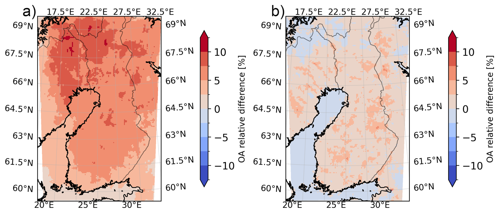
Figure 13 Relative changes in OA concentration. (a) The relative changes are calculated between baseline and MEG3-UPD. (b) The relative changes are calculated between MEG3-UPD and MEG3-UPD-CC.

4 Discussion and recommendations

In this section, we compare our results with previous studies, highlight the new insights gained, and provide recommendations for future research.

Overall, the modifications introduced here led to more realistic isoprene emissions and concentrations, and a reduction in model biases for both BVOCs and OA, even though the impact on OA is small as monoterpenes and sesquiterpenes play a larger role in OA formation. At the same time, the analysis also revealed persistent challenges, including the underestimation of OA and the incomplete representation of certain ecosystem sources, such as emissions from the forest floor and wetlands.

Our study further develops the work of Cholakian et al. (2023), which studied the influence of domain-specific land-use information on BVOC emissions simulated with MEGANv3.2. The most significant advance in this work compared to Cholakian et al. (2023) is the shift from an ecotype-based approach with constant species distributions within a given ecotype to a high-resolution representation of species distributions in the EPs calculations. In this framework, virtually every grid cell contains a unique tree species composition. Our results show that the spatial distribution of tree species strongly affects the final EPs, with variation in isoprene EPs ranging from −20 % to 20 % compared to the spatially uniform species distribution case. Additionally, our results show that incorporating information about tree-species can significantly modify EPs relative to cases where MEGAN relies solely on the needleleaf/broadleaf distinction in each ecotype. Because the standard MEGANv3.2 configuration includes species information only for the contiguous US, this limitation introduces considerable uncertainty in global applications. Future efforts should therefore prioritize the development of comprehensive, species- or at least genus-level, tree distribution datasets at the global scale. On top of that, more extensive measurements of species-specific EFs should be conducted for as many tree species as possible. Expanding the empirical basis of species-specific EFs is essential for reducing model uncertainty and improving the robustness of global and regional biogenic emissions estimates.

Improvements for future work should include extending this framework to wetlands, which are widespread across the boreal region but remain underrepresented in current emission models. High-latitude wetlands are significant sources of BVOCs, including isoprene and terpenes, and their emissions have been shown to be highly sensitive to temperature changes (Vettikkat et al., 2023). This sensitivity underscores the importance of incorporating wetlands into future studies, particularly when investigating climate–biosphere feedbacks such as the interaction between global warming and aerosol formation from natural sources.

The implementation of the canopy correction improved the simulation of in-canopy concentrations, highlighting the strong influence of the forest canopy in regulating near-surface BVOCs levels through its control on vertical mixing and advection. However, its impact on concentrations above the canopy and on regional OA levels was minor. While this may limit its importance for large-scale modelling, a canopy correction remains valuable for accurately simulating BVOCs concentrations inside the canopy, and is therefore crucial when comparing model outputs with in-canopy observations. It should also be noted that the canopy correction applied here was relatively simple, affecting only the first model layer; a more detailed representation that accounts for layers adjacent to the canopy may further enhance model performance.

Despite improved isoprene representation (MBE reduced from 0.44 ppbv in the baseline to −0.15 ppbv with all modifications), mainly due to updated emissions, and improved monoterpene representation (MBE improved from −0.45 to 0.16 ppbv), largely attributable to the canopy correction, OA concentrations remained underestimated, particularly during episodes of southerly and easterly air-mass transport. Back-trajectory analysis revealed that this bias is partially attributable to underestimated contributions from boundary conditions. Increasing the size of the model domain only partially mitigates this problem. Another factor contributing to the underestimation is the model's insufficient production of BSOA. In particular, OA concentrations in Hyytiälä were found to depend strongly on the degree to which air masses had been exposed to monoterpene emissions during the 72 h prior to their arrival. Across the full range of these exposure levels, the model systematically underestimated the resulting OA, indicating a systematic underproduction of BSOA under the typical conditions found in the boreal region. Numerous factors can contribute to this underproduction. For instance, in the model, the oxidation products of different BVOCs are distributed into four volatility classes based on their C^*, with the lowest C^* of 1 µg m⁻³ corresponding to what is typically defined as semi-volatile organic compounds (SVOCs). However, low-volatility (LVOCs), extremely low-volatility (ELVOCs), and ultralow-volatility (ULVOCs) organic compounds have been shown to be critical for the growth of aerosols to sizes at which SVOCs can effectively condense (Jokinen et al., 2015; Stolzenburg et al., 2023; Dada et al., 2023; Lopez et al., 2025). The absence, or too simplistic representation, of LVOCs, ELVOCs, and ULVOCs can therefore lead to two main issues: (i) a direct underestimation of condensable gases, resulting in underestimated BSOA production, and (ii) limited growth of freshly nucleated particles, which indirectly reduces BSOA by underestimating the number of particles large enough for SVOCs to condense onto.

Additionally, our results confirm earlier findings that isoprene reduction can increase OA production under certain conditions, due to reduced scavenging of OH radicals and enhanced oxidation of monoterpenes. However, it is important to acknowledge that this result might be biased by the chemical mechanism used in this study. In particular, missing OH-recycling pathways in isoprene oxidation can reduce modelled OH levels and slow down isoprene loss, contributing to positive concentration biases under low-NO_x conditions (Wennberg et al., 2018). This effect is expected to be relevant in boreal environments and should be considered when interpreting model–measurement discrepancies. Specifically, because the chemical mechanism used in this study underrepresents OH recycling during low-NO_x isoprene oxidation, it likely overestimates the OH-scavenging effect of isoprene. As a result, the simulated enhancement of monoterpene oxidation and OA formation following isoprene emission reductions likely represent an upper-bound response relative to simulations using more recent isoprene chemistry.

Based on these findings, we make the following recommendations for future studies:

• For BVOCs emissions estimation, incorporating high-resolution species distribution information is highly recommended over uniform distribution for each ecotype. If this is not possible, including all the main tree species or genera (with uniform distribution) present in a given ecotype should be preferred over the simple needleleaf/broadleaf classification.

• BVOCs emissions from wetlands should be included in future studies, ideally following the same framework presented in this study.

• When performing simulations over domains including forests, we recommend including the forest canopy effect on vertical diffusivity and wind speed. This is especially important when evaluating models with observations inside the canopy, as the absence of a canopy correction would significantly influence the model output in the layers inside the canopy. This has also been noted by Cholakian et al. (2023).

• A more detailed representation of the physicochemical properties of organic compounds should be incorporated. In particular, LVOCs, ELVOCs, and ULVOCs should also be explicitly included in atmospheric models. While a few CTMs already account for this process, big uncertainties remain, and this will require additional efforts from laboratory studies to better constrain the key reaction pathways and their corresponding yields.

5 Conclusions

This study evaluated a regionally customized implementation of the MEGAN model for boreal forests and its impact on BVOC emissions and SOA formation in Finland. Updated tree species distributions and species-specific EFs improved isoprene emission calculations, substantially reducing the historical high bias.

Adding a canopy correction for wind and vertical mixing improves BVOC concentration estimates within the forest canopy and aligns better with in-canopy measurements. This correction has little impact above the canopy, so its main value is for comparing in-canopy observations with models.

Lower isoprene emissions increase OA in large parts of Finland by reducing competition with monoterpenes for the OH radical, however, the model still underestimates OA. Back-trajectory analysis shows that the largest underestimation occurs when air masses originate from the south and east, areas with higher monoterpene emissions. The model's OA response to monoterpene exposure is reasonable but underestimated, suggesting underproduction of BSOA. Better representation of LVOC, ELVOC, and ULVOC formation and fate could improve model performance.

Overall, the study identifies three elements important for improved BVOC–aerosol modelling in boreal environments and globally: (i) detailed tree species distributions, (ii) accurate representation of canopy mixing, and (iii) chemical mechanisms for forming low-volatility products from BVOCs. Adding other BVOC sources like wetlands will further improve regional and global aerosol–climate assessments.