NO_x emissions constraints from GEMS NO₂ retrievals: inversion methodology and air quality model evaluation in Bangkok using ASIA-AQ multi-platform observations

Nitrogen Dioxide (NO₂) is a key component of tropospheric chemistry and air quality, yet large uncertainties persist in regional NO_x emissions across rapidly developing megacities in Southeast Asia. Observations from the Geostationary Emissions Monitoring Spectrometer (GEMS) provide new constraints on anthropogenic NO₂ variability, while the 2024 NASA Airborne and Satellite Investigation of Asian Air Quality (ASIA-AQ) campaign, offers an extensive, independent dataset for model evaluation. Here, we examine air quality in Bangkok using coarse (20 km) and high-resolution (4 km) WRF-Chem simulations during ASIA-AQ. We develop a top-down framework that uses hourly GEMS NO₂ columns to derive constraints on the daytime cycle of NO_x emissions. Emissions are first estimated from GEMS using a Cross-Sectional Flux (CSF) inversion and then incorporated into WRF-Chem through a novel optimization that reshapes the magnitude and daytime structure of NO_x while accounting for lifetime and satellite vertical sensitivity. GEMS-constrained NO_x emissions for March 2024 are estimated to range from 2.7 to 4.3 kt month⁻¹ after accounting for known low biases in the GEMS retrievals. Re-running WRF-Chem with the updated emissions leads to substantial improvements in modeled NO₂ magnitude and temporal variability when evaluated against independent ground-based, Pandora, and airborne measurements. Remaining negative biases are consistent with a systematic low bias in the GEMS v3 NO₂ product, highlighting the importance of multi-platform evaluation using independent observations. Together, these results demonstrate the value of hourly geostationary observations combined with high-resolution modeling as a scalable pathway for improving urban NO_x emissions estimates and air quality simulations in Southeast Asia.

1 Introduction

The troposphere contains a variety of pollutants and aerosols that degrade air quality and affect human health (Chen and Chen, 2021; Fuller et al., 2022; Shetty et al., 2023). Nitrogen oxides (NO_x= NO + NO₂) are primary pollutants with significant variability in space and time (Seinfeld and Pandis, 2016). Information on NO_x sources is crucial in defining its concentration and distribution (Miyazaki et al., 2019). Nitrogen dioxide (NO₂) is fundamental to air quality and atmospheric chemistry, as it is the primary precursor to surface ozone (O₃) and nitrate aerosols (Pörtner et al., 2022) and is independently linked to the development of pediatric asthma (Anenberg et al., 2022). It is thus inherent that NO₂, and its sources, are well quantified and studied to gain insights into its environmental impact.

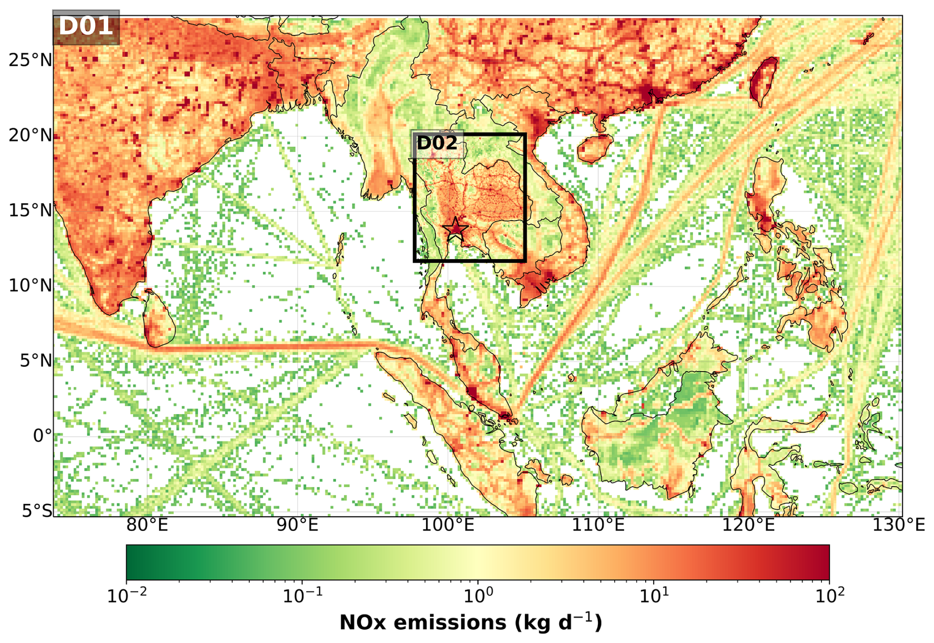
Figure 1 Spatial illustration of the WRF-Chem model domain configuration, including D01 (20 km) and D02 (4 km), and average base-model NO_x input emissions from EDGAR v5. D02 is centered over Thailand, and the urban signal associated with the Bangkok Metropolitan Region (BMR) is highlighted by the star.

Over the past two decades, satellite observations of tropospheric NO₂ have revealed substantial regional variability in emissions, particularly over industrial and urban areas (Goldberg et al., 2024; Park et al., 2025; Rey-Pommier et al., 2025). While strict air quality policies in North America and Europe have resulted in significant NO₂ reductions, many developing regions, especially the megacities of Southeast Asia, have seen increases (Elguindi et al., 2020; Georgoulias et al., 2019; Miyazaki et al., 2017; Park et al., 2025; Sicard et al., 2023). Thailand, for example, has undergone rapid industrialization, urbanization, and economic growth over the past 30 years, with most of this development occurring in the Bangkok Metropolitan Region (BMR) (Thailand Office of the National Economic and Social Development Board; World Bank, 2017; Uttamang et al., 2018). This has led to increased emissions from vehicular traffic and industrial activity, resulting in a sustained degradation of air quality (Uttamang et al., 2018). Since the mid-1990s, the BMR has frequently exceeded Thailand's National Ambient Air Quality Standards (NAAQS) for particulate matter (PM) (25 µg m⁻³) and O₃ (100 ppb), particularly during the dry season (February–May) (Kumar et al., 2012; Uttamang et al., 2018, 2020, 2023). Within the BMR, there have been initiatives to reduce health impacts and exposure related to PM_2.5. For example, the National Agenda Action Plan on “Solving the Pollution Problems of Particulate Matter” motivated implementation measures in transport, industry, and waste sectors (Aung et al., 2025). However, achieving the air quality standard has remained an issue. Modeling studies have shown that O₃ levels typically peak between January and March, coinciding with increased solar radiation, higher temperatures, elevated humidity, and prevailing northeasterly winds during the Northeast monsoon season. These meteorological conditions, combined with rising emissions, often contribute to O₃ pollution episodes in the region (Uttamang et al., 2020). A key limitation of these air quality modeling studies is the uncertainty in bottom-up anthropogenic emissions inventories, which remain a significant source of error. In the BMR, uncertainties in regional emissions can be as large as a factor of 2 or higher (Bond et al., 2004, 2007; Smith et al., 2011; Uttamang et al., 2020). These emissions uncertainties limit our ability to accurately simulate pollutant concentrations and assess the effectiveness of emission control strategies. Thus, to address this issue, new observational capabilities that can directly capture emission variability at fine spatial (< 10 km) and temporal (hourly) scales are needed.

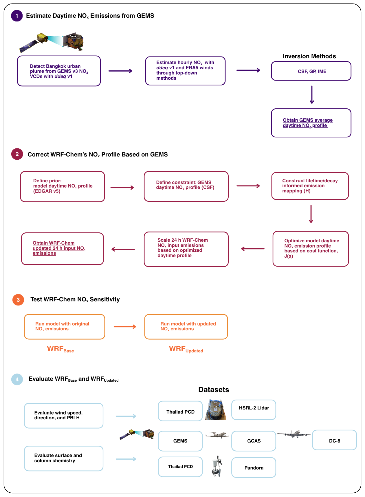
Figure 2 Schematic overview of the workflow used to derive satellite-constrained daytime NO_x emission profiles and assess their impact in WRF-Chem over the BMR. (1) Urban NO₂ plumes are detected using GEMS tropospheric NO₂ columns, and hourly NO_x emissions are estimated using top-down methods implemented in the ddeq v1 Python library. (2) A GEMS-derived daytime NO_x profile is used to constrain the prior emission profile through an optimization framework, yielding updated input 24 h NO_x emissions for WRF-Chem. (3) Model simulations are performed using both the original and updated emissions. (4) Model performance is evaluated against surface, column, airborne, and observations.

We are currently entering a new era of satellite atmospheric composition monitoring with the launch of three geostationary (GEO) imaging spectrometers covering a large component of the Northern Hemisphere. The Geostationary Environmental Monitoring Spectrometer, GEMS (Kim et al., 2020), Tropospheric Emissions: Monitoring of Pollution, TEMPO (Zoogman et al., 2017), and Sentinel-4 (Gulde et al., 2017), now provide unprecedented spatial and temporal resolution of atmospheric constituents. These instruments offer hourly observations that resolve daytime variability of key pollutants, including NO₂. Until now, most studies of top-down NO_x emissions have relied on once-daily measurements from low Earth orbit (LEO) satellites (i.e., OMI, TROPOMI) requiring assumptions about diurnal emission and chemistry patterns that introduce uncertainties when coupled with chemical transport models, particularly those arising from coarse spatial resolution (> 20 km), emissions inventories, and chemical mechanisms (Park et al., 2025). Although these measurements have been invaluable for global and long-term NO_x assessments, they cannot fully capture the pronounced sub-daily variability in NO₂ driven by emissions, chemistry, and transport. GEO satellites now provide the capability to directly observe this hourly variability (Park et al., 2025). For example, using 12 km WRF-Chem simulations Hsu et al. (2026) showed that TEMPO-derived top-down NO_x emissions are broadly consistent with TROPOMI and bottom-up inventories, but noted coarse model resolution (e.g., 12 km) can limit the representation of coastal meteorology and chemical nonlinearity.

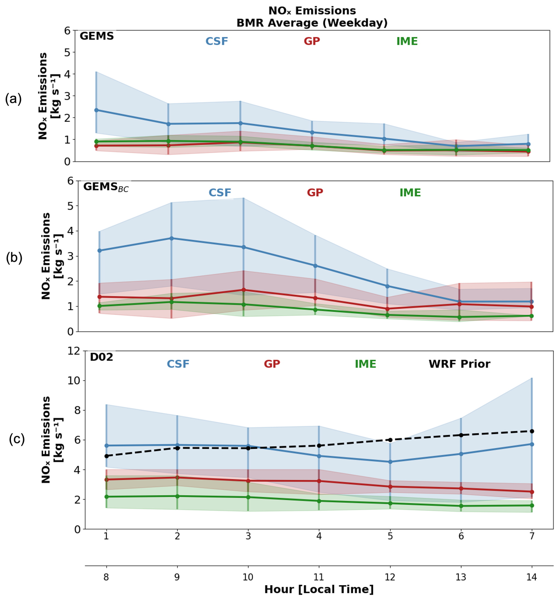
Figure 3 Comparison of daytime NO_x emission estimates derived from (a) GEMS, (b) GEMS with bias correction applied (GEMS_BC), and (c) WRF-GEMS D02 using the Cross-Sectional Flux (blue), Gaussian Plume inversion (red), and Integrated Mass Enhancement (green) methods. Emissions (kg s ⁻¹) represent averages across daytime hours and weekdays during the ASIA-AQ deployment period (14–27 March 2024). Model-derived emissions in (c) were obtained by re-gridding WRF_Base output to the GEMS spatial resolution and applying the same inversion methods. The WRF_Base prior emission profile is shown as a black dashed line and represents a backward-looking 3 h average to account for emission accumulation embedded in the inversion estimates.

GEMS was the first UV-visible hyper-spectrometer in geostationary orbit and was launched on GEO-KOMPSAT-2B on 18 February 2020. GEMS measurements allow the observation of air quality constituents (e.g., NO₂, SO₂, O₃, HCHO, CHOCHO, and aerosols) at a spatial resolution of 3.5 km ×7.7 km² at the center of its field of regard and was the first space-based instrument to provide hourly observations of these species. The GEMS field of regard covers 20 countries in Asia, E–W from Japan to India, and N–S from Mongolia to Indonesia (Kim et al., 2020; Park et al., 2025). Recent work has demonstrated the potential of GEMS and air quality models to estimate top-down NO_x emissions over major Asian cities during the summertime (de Foy and Schauer, 2022; Park et al., 2024, 2025). These studies highlight the need for comprehensive validation involving independent observations. The Airborne and Satellite Investigation of Asian Air Quality, ASIA-AQ, has provided an excellent opportunity to conduct extensive validation of air pollutants across multiple Asian megacities, including Bangkok (ASIA-AQ White Paper) (ASIA-AQ, 2025).

In this manuscript, we aim to address these gaps specifically near Bangkok, Thailand by deriving emissions and examining fine- (4 km) and coarse- (20 km) resolution Weather Research and Forecasting model coupled with Chemistry (WRF-Chem) simulations driven by them during mid-March 2024. First, we derive daytime hourly NO_x emissions from GEMS over the BMR in March 2024. Next, we use the GEMS emissions to constrain hourly model emissions through a novel optimization technique. To conclude, we assess model performance using GEMS and independently with ground-monitor information, Pandora site measurements, and airborne measurements collected during the ASIA-AQ campaign.

Table 1 WRF-Chem base (WRF_Base) model configuration and input datasets.

2 Model configuration and experimental design

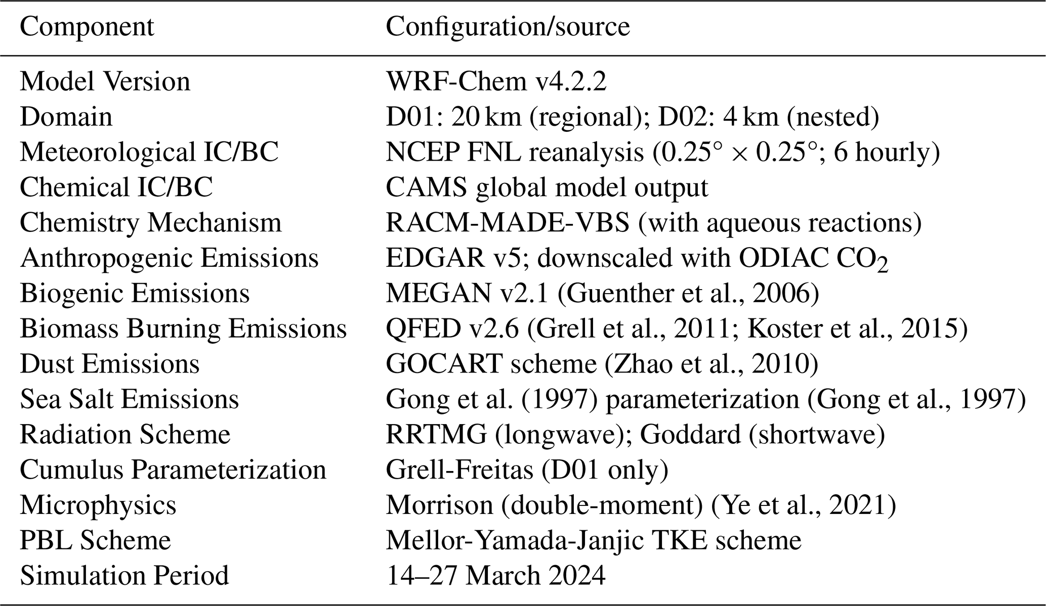
To simulate air quality over the BMR, we use a regional simulation of WRF-Chem v4.2.2 in a research configuration (Table 1; Fig. 1) (Agarwal et al., 2024; Anav et al., 2024; Gao and Zhou, 2024; Skamarock et al., 2019). The model setup follows previous WRF-Chem implementations in the Korea-United States Air Quality field study (KORUS-AQ) for air quality studies over the Seoul Metropolitan Area (Choi et al., 2020; Goldberg et al., 2019; Lennartson et al., 2018; Park et al., 2021; Saide et al., 2020). The model was driven by reanalysis meteorology, NCEP Final Reanalysis (NCEP FNL), and Copernicus Modeling Service (CAMS) chemical boundary conditions (National Centers for Environmental Prediction/National Weather Service/NOAA/US Department of Commerce, 2000; Inness et al., 2019). Meteorology was constrained using four-dimension data assimilation (FDDA) via grid nudging applied to model domains using the 0.25° NCEP FNL reanalysis fields to improve large-scale wind representation. A two-domain approach with one-way nesting was incorporated to gauge strengths between coarse- and high-resolution simulations. D01 (20 km) spans a large portion of the GEMS field of regard, covering primary transboundary pollution sources (e.g., deserts in China/India, anthropogenic emissions from China/India). A nested 4 km domain (D02) is centered over Bangkok (Fig. 1).

Original anthropogenic emissions of trace gases and primary aerosols were based on the Emissions Database for Global Atmospheric Research (EDGAR v5) (Crippa et al., 2020) inventory at 0.1°×0.1° horizontal resolution. For D02, EDGAR emissions for the transport and industrial sectors were downscaled using the Open-source Data Inventory for Anthropogenic Carbon Dioxide emission inventory (ODIAC) at 1 km × 1 km resolution (Oda et al., 2018). This is done by distributing EDGAR emissions into the 1 km² grid using ODIAC CO₂ as a spatial proxy in a mass conserving way. Biogenic, dust, sea salt, and fire emissions were computed within WRF-Chem using the model's full-chemistry emission modules (Table 1). In this configuration, dust and sea-salt emissions are calculated every chemistry timestep, while biogenic emissions (MEGAN) are updated every 30 min. For fire emissions, plume rise is enabled, in which the injection heights are diagnosed using the plume-rise parameterization and emissions are vertically distributed (typically ∼ 80 % at the surface with the remainder aloft). The model was configured using the RACM-MADE-VBS (Ahmadov et al., 2012; Tuccella et al., 2015) chemical mechanism and physics parameterizations selected based on prior campaign experience (e.g., KORUS-AQ), with updates to better represent secondary organic aerosol formation, heterogenous chemistry, and aerosol properties. The modal aerosol scheme in MADE-VBS tracks both particle mass and number, allowing mode diameters to evolve dynamically with aerosol aging and growth processes. Hereafter, we will refer to this model configuration as WRF_Base. Model cases with updated anthropogenic NO_x emissions will be referred to as WRF_Updated and WRF_Updated+BC (later introduced).

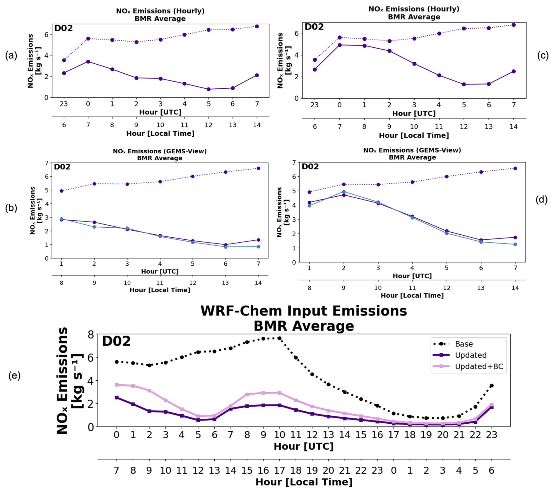
Figure 4 Results of the emissions optimization, shown as averages over the BMR. (a) Posterior optimized (solid) and prior (dashed) daytime NO_x emissions in model space, where the prior represents the 3 h backward average of EDGAR v5 emissions used as input to the optimization. (b) Same emissions as in (a) but transformed into observational space using the observational operator. The GEMS profile is shown in blue. (c) and (d) are representative of optimization results using the GEMS bias-corrected CSF results as the constraint. (e) Full diurnal cycle of updated (solid purple), updated+BC (solid pink), and prior (dashed) NO_x emissions. Note that, unlike (a), the prior in (e) does not include the 23 UTC hour from the previous day in the backward averaging.

3 Satellite-derived NO_x emission estimates

3.1 Correcting for GEMS bias prior to inversion

Recent independent validation studies of the operational GEMS v3 product over Bangkok and South Korea report low biases in NO₂ columns relative to ground-based sun-photometer and DOAS measurements (Bae et al., 2025; Jung et al., 2025). Bae et al. (2025) shows that GEMS v3 increasingly underestimates NO₂ relative to Pandora under high-NO₂ conditions ($>\mathrm{1}\times {\mathrm{10}}^{\mathrm{16}}$ molecules cm⁻²) as is the case for Bangkok pollution levels. In Jung et al. (2025), validation results over Bangkok indicate a pronounced low bias in GEMS tropospheric NO₂ columns relative to Pandora, with regression slopes of ∼ 0.35 for v2.0 and ∼0.28 for v3.0, indicating increasing underestimation at higher NO₂ levels. While moderate correlations (r ≈ 0.6–0.7) suggest that GEMS captures temporal variability, column magnitudes are substantially underestimated, particularly under polluted conditions. The persistence of this behavior in the v3.0 product indicates that the low bias is not fully corrected by recent algorithm updates and is consistent with retrieval sensitivity limitations in highly polluted urban environments (Jung et al., 2025).

To address the low bias in GEMS prior to the NO_x satellite emission inversion, we first quantify the GEMS bias relative to Pandora measurements over our period of interest (14–27 March 2024). We compare total column GEMS NO₂ to Pandora Level 2 direct-sun total column retrieval, filtering for high quality measurements (quality flag = 10) and averaging to hourly means. GEMS columns are sampled at the nearest grid cell to each Pandora site and temporally collocated. Results are shown in Fig. S1 in the Supplement. GEMS NO₂ columns are generally about a factor of two lower than Pandora measurements (mean bias $\approx -\mathrm{9.2}\times {\mathrm{10}}^{\mathrm{5}}$ molecules cm⁻²). This factor-of-two difference persists throughout March 2024 (Fig. S1).

To assess the sensitivity of the top-down NO_x inversion framework to this bias, we apply a simple correction factor to GEMS prior to inversion. Specifically, GEMS NO₂ columns over the BMR are scaled by a factor of 1.67 derived from the Pandora comparison. The inversion is then performed with and without the bias-corrected columns.

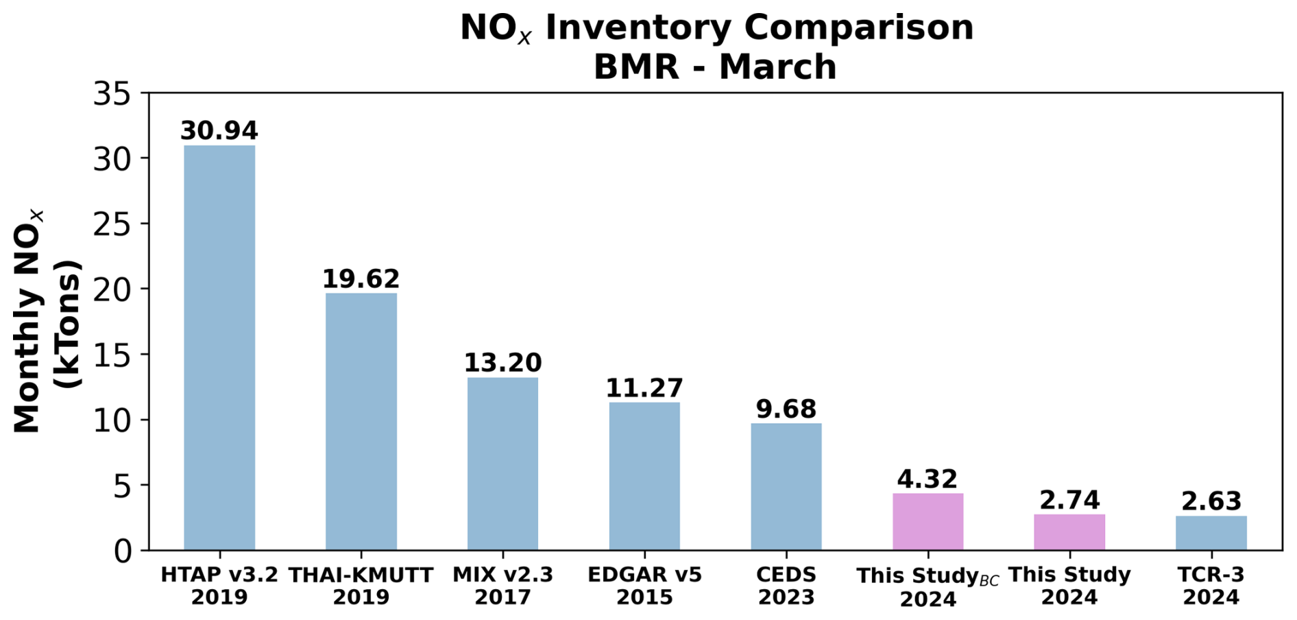
Figure 5 Comparison of March NO_x emissions over the BMR derived from bottom-up, top-down, and assimilated approaches. Bottom-up inventories (HTAP v3.2; Guizzardi et al., 2025), THAI-KMUTT, MIX v2.3 (Li et al., 2024), EDGAR v5 (Crippa et al., 2020), and CEDS (Hoesly et al., 2018)) exhibit substantial variability. In contrast, top-down estimates from GEMS and TROPOMI (TCR-3) for 2024 indicate considerably lower emissions (2.6–4.3 kt month⁻¹), highlighting uncertainties in bottom-up inventory methodologies, satellite sensitivity, and potential changes in anthropogenic NO_x activity.

3.2 GEMS inversion framework

Previous studies have used satellite data (OMI, TROPOMI, SCIAMACHY, GOME (−2), OMPS) to estimate top-down NO_x emissions over urban areas, but were limited to once-a-day, mid-afternoon measurements, leaving temporal variability in emissions largely unaddressed (Beirle et al., 2011; Goldberg et al., 2017, 2019). Ground-based and aircraft measurements of emissions can be challenging to constrain given boundary layer dynamics, such as changes in boundary layer height, stability, and vertical mixing, which can strongly influence observed concentrations of trace gases (Goldberg et al., 2017, 2019). Additionally, temporal allocation in bottom-up emission inventories remain a significant uncertainty, particularly at hourly and daily timescales because default temporal profiles (diurnal, weekly, seasonal) often fail to capture real activity patterns, meteorological influences, and sector-specific variability (Goldberg et al., 2017, 2019; Mues et al., 2014). GEMS observations, however, offer a unique opportunity to provide hourly emissions rates over Bangkok, complementing existing inventories that are usually provided at monthly scales. To estimate NO_x emissions over Bangkok in March 2024, we apply the methodology of Kuhlmann et al. (2024), implemented through the openly available data-driven emission quantification (ddeq v1) Python library (see step 1, Fig. 2). The standard ddeq library implements computationally inexpensive methods (e.g., Gaussian Plume Inversion (GP), Cross-Sectional Flux (CSF) method, Integrated Mass Enhancement (IME) method) to estimate emissions from Sentinel5P TROPOMI images (Graziosi and Manca, 2025; Meier et al., 2024). One study found limited temporal sampling from polar-orbiting satellites (i.e., TROPOMI) can lead to systematic underestimation of NO_x emissions, particularly because wintertime conditions with higher emissions are often poorly observed due to cloud cover (Meier et al., 2024). Geostationary observations, including GEMS, address this limitation by providing hourly measurements that increase the likelihood of usable data on partially cloudy days and enable direct resolution of daytime emission variability, which is not accessible from once-daily LEO observations. For our application, we estimate emissions for daylight hours from GEMS tropospheric column NO₂ data over Bangkok during the ASIA-AQ campaign. A brief description of inversion methods and specifics is provided here. A complete description of the inversion methods and algorithm can be found in Kuhlmann et al. (2024).

First, within the ddeq framework, the source location (Bangkok; 13.7563° N, 100.5018° E), GEMS v3 NO₂ column data, and ERA5 wind fields are read. We chose to incorporate ERA5 wind fields as opposed to those provided by our high resolution WRF-Chem simulation in this analysis given they presented significantly lower bias when compared to surface observations (Fig. S2; Sect. 6.1). The ERA5 wind fields were downloaded and prepared by the ddeq library. Cloudy pixels (CF > 0.3) were removed. Next, a plume detection algorithm is implemented to identify the Bangkok urban plume within the GEMS image. The Bangkok plume subregion is estimated based on the source location and ERA5 wind field. Generally, a wind vector is taken at the source location, and the plume is assumed to be located downwind, and a rectangular polygon can be drawn with the along- and across-wind direction (Kuhlmann et al., 2024). An example of these plume detections and associated rectangular polygons is shown in Fig. S3. To aid the algorithm's plume detection process, we identify two additional sources north of Bangkok in the Saraburi province to avoid overlapping plumes from other NO_x sources. These correspond to the Khao Wong (14.692856° N, 100.817204° E), and Thap Kwang (14.645313° N, 101.077650° E) regions, which we identified through NO₂ patterns visible in the GEMS data in Fig. S3. These areas are not representative of Bangkok urban emissions as they are a source of industrial activity related to limestone quarries and mining operations outside the inversion domain (Makkwao and Prueksasit, 2021). Next, a center curve is fitted to the data, and natural coordinates are calculated for the detected plume associated to Bangkok to prep for the inversion algorithm. The coordinates are computed as the distance along and perpendicular to the wind vector and for curved plumes this distance is computed as the arc length. Lastly, the data is prepared for the satellite-derived emissions estimation by calculating and removing the background field and converting the NO₂ columns to kg m⁻². We estimate satellite-derived NO_x emissions using three inversion techniques included in ddeq: CSF, GP, and IME methods. Below is a summary of the CSF method defined in Kuhlmann et al. (2024). GP and IME method descriptions are available in the Supplement (e.g., S1) and Kuhlmann et al. (2024). In the following subsections and in Sect. 4, we refer to the WRF-Chem input inventory based on EDGAR as the prior emissions, the CSF-based estimates from GEMS as the satellite-derived emissions, the CSF-based estimates from the model-simulated columns as the model-derived emissions, and the final emissions after applying the optimization framework, as the posterior emissions.

3.3 Cross-Sectional Flux (CSF) framework

The CSF approach applies mass conservation to quantify the NO_x flux transported downwind of Bangkok using (i) the wind speed perpendicular to the plume and (ii) the NO₂ enhancement integrated along the plume (line density). The NO_x flux, F (kg s⁻¹), is defined as:

$$\begin{array}{}\text{(1)}& F=u\cdot q\end{array}$$

where u (m s⁻¹) is the effective transport wind speed and q (kg m⁻¹) is the NO₂ line density. The emission rate, Q (kg s⁻¹), is then inferred by correcting for chemical decay along the plume using:

$$\begin{array}{}\text{(2)}& Q={\displaystyle \frac{F\left(x\right)}{D(x,\mathit{\tau })}}\end{array}$$

Here, D(xτ) represents the along-plume decay for lifetime τ. Here, τ represents an effective plume lifetime that accounts for both chemical decay and plume dispersion (Kuhlmann et al., 2024).

3.3.1 Effective wind speed estimation

The ddeq algorithm computes an effective wind speed, i.e., the plume-transport wind, that supports an unbiased emission estimate. Ideally, this is a NO₂-enhancement-weighted average of the along-plume wind:

$$\begin{array}{}\text{(3)}& u(x,y)={\displaystyle \frac{{\int }_{\mathrm{0}}^{z_{\mathrm{T}}}{\mathit{\rho }}_e(x,y,z)u(x,y,z)\mathrm{d}z}{{\int }_{\mathrm{0}}^{z_{\mathrm{T}}}{\mathit{\rho }}_e(x,y,z)\mathrm{d}z}}\end{array}$$

Here, ${\mathit{\rho }}_e(x,y,z)$ is the NO₂ enhancement, $u(x,y,z)$ is the along-plume wind speed and z_T is the plume-top height. Because ρ_e is not directly observed, ddeq follows the approximation of Fioletov et al. (2015), in which the effective wind speed is estimated using the mean of the lowest three ERA5 layers, representing the typical transport level for near-surface urban plumes.

3.3.2 NO₂ line density calculation

The line density q(x), is the integral of the NO₂ enhancement across the plume cross-section:

$$\begin{array}{}\text{(4)}& q\left(x\right)={\int }_{y_{\mathrm{1}}}^{y_{\mathrm{2}}}\left(V(x,y)-V_{\mathrm{bg}}(x,y)\right)\mathrm{d}y\end{array}$$

where $\left(V(x,y)-V_{\mathrm{bg}}(x,y)\right)$ represents the NO₂ enhancement above the background in kg m⁻². The integration bounds y₁ and y₁ are defined by the plume subregion (polygon) identified using the ddeq framework, which delineates the area of enhanced NO₂ associated with the source based on plume detection and wind direction (Kuhlmann et al., 2024). As such, the effective integration length across the plume is determined by the spatial extend of this polygon and the fitted Gaussian representation. To further compute this and account for missing satellite pixels, ddeq fits a Gaussian function to all GEMS pixels within a plume polygon:

$$\begin{array}{}\text{(5)}& g\left(y\right)={\displaystyle \frac{q}{\mathrm{2}\sqrt{\mathit{\pi }\mathit{\sigma }}}}\exp \left(-{\displaystyle \frac{{\left(y-\mathit{\mu }\right)}^{\mathrm{2}}}{\mathrm{2}{\mathit{\sigma }}^{\mathrm{2}}}}\right)+my+b\end{array}$$

Here, μ and σ(x) are the plume center and width in meters, and my+b approximates a linear background. The plume width is further defined as:

$$\begin{array}{}\text{(6)}& \mathit{\sigma }\left(x\right)=\sqrt{{\displaystyle \frac{\mathrm{2}Kx{}^{\mathit{\kappa }}}{u}}}\end{array}$$

where K is the eddy diffusivity coefficient (m² s⁻¹), κ accounts for nonlinear plume spreading under varying meteorology, and u is the effective transport wind speed defined above. The plume width, σ(x) is derived from the Gaussian fit, and the parameters, K and κ are then determined by fitting, σ(x) within the CSF framework. After fitting the Gaussian function, line densities are converted to fluxes using wind speeds at each corresponding downwind cross-section. Fluxes can be estimated for several cross-sections or polygons located downwind of the urban source (see Figs. S3, S4) (Kuhlmann et al., 2024). Using multiple points along the plume ensures different portions of the plume are sampled robustly.

3.3.3 Emission rate and lifetime estimation

Because NO₂ decays as the plume travels, the flux decreases with distance. To estimate the true emission rate, Q, at the source, ddeq fits a lifetime τ by matching modeled and observed flux decay:

$$\begin{array}{}\text{(7)}& F_a\left(x,\mathit{\tau },{\mathit{\mu }}_a,{\mathit{\sigma }}_a\right)=Q{\int }_{-\mathrm{\infty }}^{\mathrm{\infty }}D\left(x^{\prime },\mathit{\tau }\right)g(x-x^{\prime },{\mathit{\mu }}_a,{\mathit{\sigma }}_a)\mathrm{d}{x}^{\prime }\end{array}$$

where μ_a and σ_a describe the city-scale plume location and extent, $D(x^{\prime },\mathit{\tau })$ describes the exponential decay along the plume, and g is the Gaussian parameter described above. Fitting Eq. (7) to the derived fluxes yields both the emission rate Q and plume lifetime τ (Kuhlmann et al., 2024).

3.3.4 Conversion from NO₂ to NO_x emissions

GEMS provides NO₂ column densities; therefore, a NO₂ to NO_x conversion factor is needed to obtain NO_x emissions. Following the ddeq implementation, we use:

$$\begin{array}{}\text{(8)}& Q_{{\mathrm{NO}}_x}=f_q\cdot Q_{{\mathrm{NO}}_{\mathrm{2}}}\end{array}$$

to obtain NO_x estimates, where f_q= 1.32, as implemented in the ddeq algorithm; a localized factor was not derived from WRF-Chem due to known NO₂ biases in the prior simulation that would propagate into the conversion.

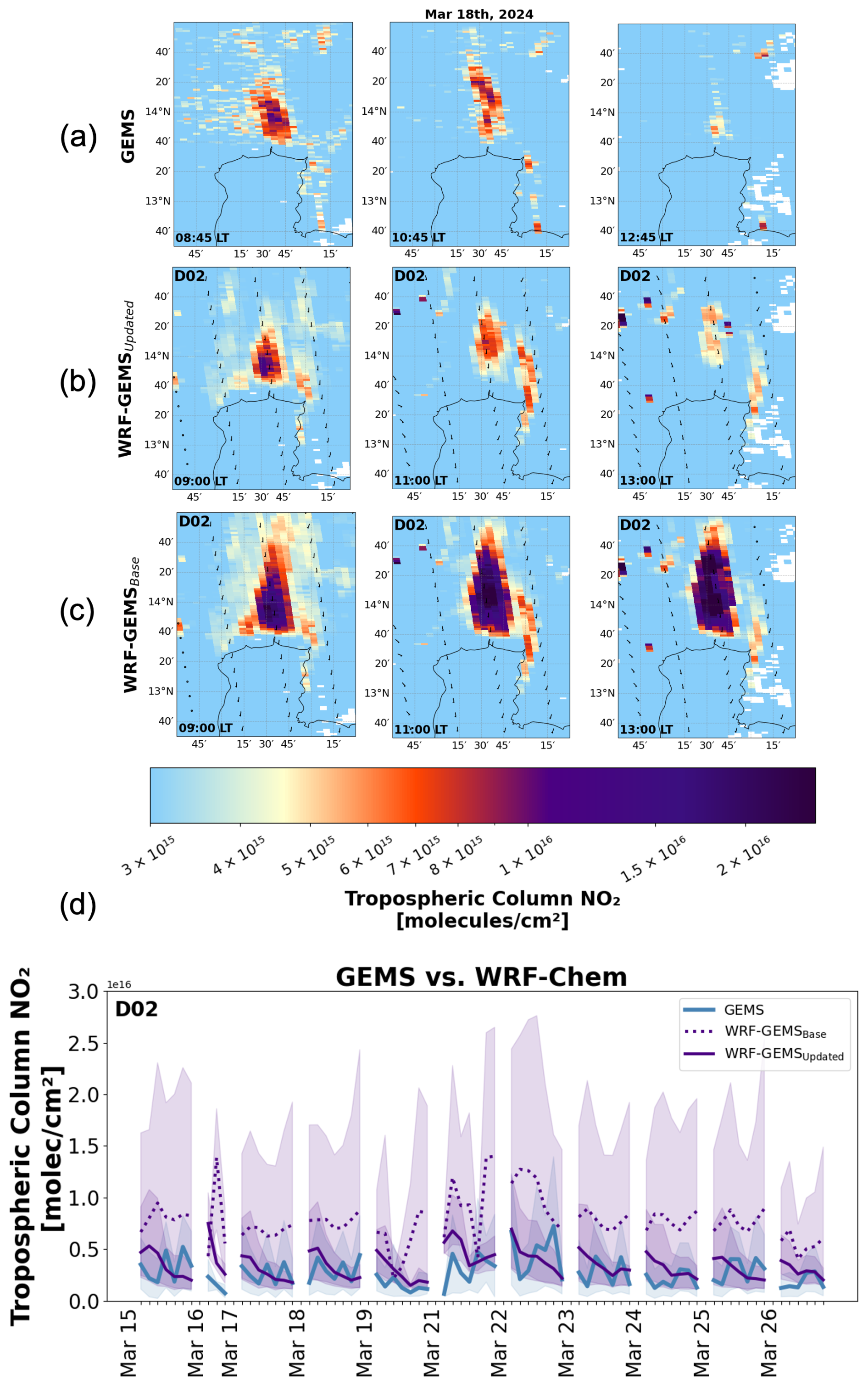
Figure 6 Spatial comparison over the BMR on 18 March 2024 of tropospheric NO₂ columns from (a) GEMS, (b) WRF-GEMS_Updated D02, and (c) WRF-GEMS_Base D02 for snapshots at 02:00, 04:00, and 07:00 UTC, corresponding to approximately 09:00, 11:00, and 13:00 LT. (d) Tropospheric NO₂ column for daytime hours between GEMS (blue), WRF-GEMS_Base D02 (dotted purple), and WRF-GEMS_Updated D02 (solid purple) during the ASIA-AQ deployment period. Shaded regions indicate variability, represented by the 10th and 90th percentiles.

3.3.5 Structural uncertainties in the CSF framework

While the CSF framework provides a computationally efficient approach for deriving satellite-derived emissions, we acknowledge the method contains some structural uncertainties. First, the integration bounds used to compute the line densities (Eq. 4) are defined by the plume polygon identified from the satellite observations and wind field, such that the inferred top-down emissions depend on how the plume extent is delineated. As a result, inferred satellite-derived emissions can be sensitive to the selected plume extent, particularly under conditions of weak enhancements or overlapping sources. Second, the satellite-derived emission estimate scales directly with the effective wind speed (Eq. 1), such that errors in wind magnitude or direction propagate into the derived fluxes and satellite-derived emissions (see Fig. S5). Although ERA5 winds averaged over the lowest model layers are used to approximate plume transport, they may not fully represent local meteorological variability. Third, the inferred satellite-derived emission rate depends on the assumptions within the fitting framework, including the Gaussian representation of plume structure (Eq. 5), the parametrization of plume spreading (Eq. 6), and the effective lifetime τ (Eq. 7), which represent a simplified treatment of chemical decay and dispersion. Together, these factors represent inherent uncertainties in the CSF approach that should be considered when interpreting the satellite-derived emissions.

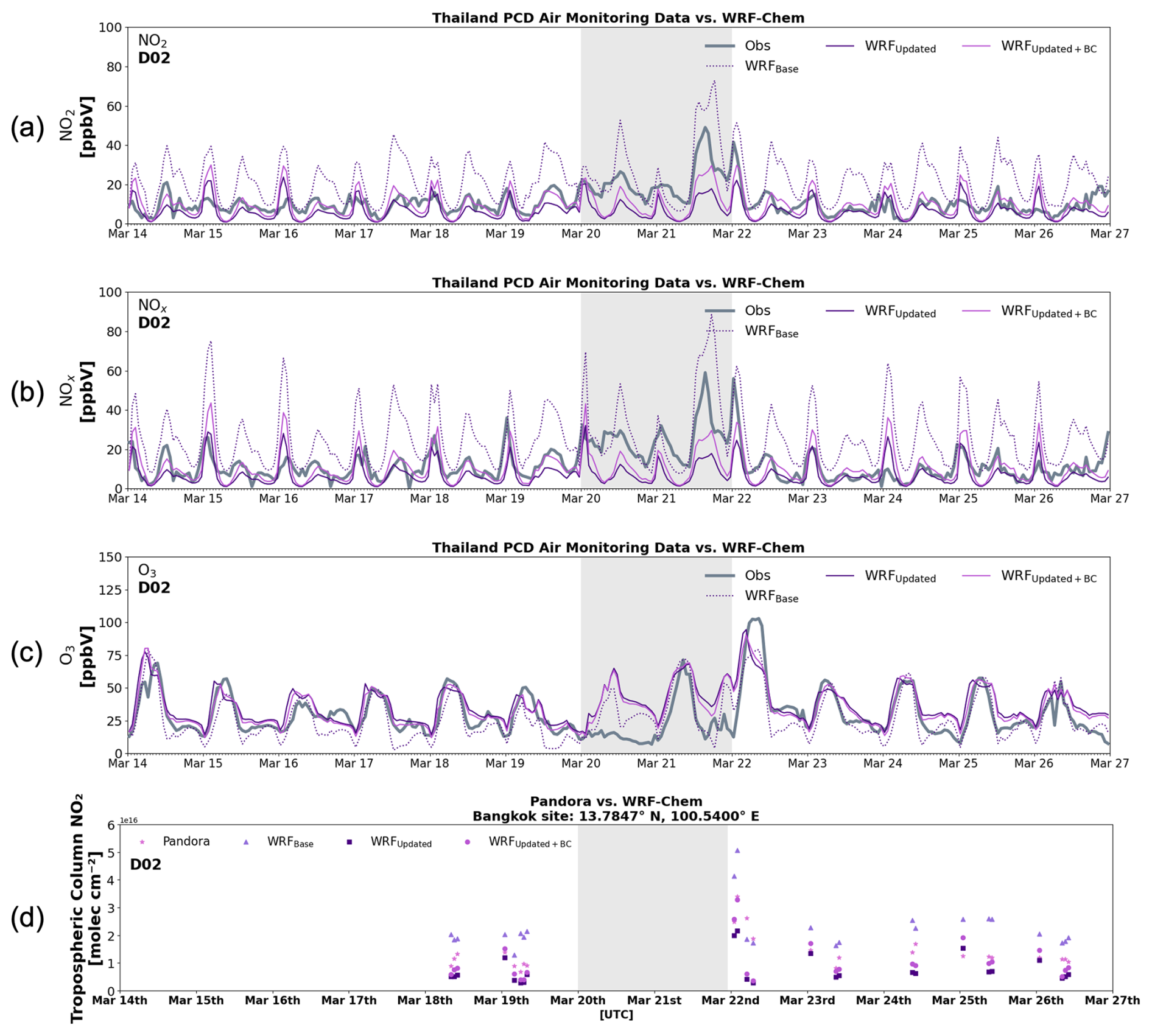
Figure 7 Comparison of WRF_Base D02 (dotted purple),WRF_Updated D02 (solid purple), and WRF_Updated+BC D02 (solid magenta) simulations against Thailand Pollution Control Department (PCD) ground-monitor network observations for (a) NO₂ mixing ratio (ppbV), (b) NO_x mixing ratio (ppbV), and (c) O₃ mixing ratio (ppbV) during the ASIA-AQ deployment period (14–27 March 2024) represent averages across stations within the Bangkok urban plume. (d) Comparison of tropospheric NO₂ columns from WRF_Base D02 (light purple triangles), WRF_Updated D02 (dark purple squares), WRF_Updated+BC D01 (magenta dots) and Pandora (pink stars) for high-quality observations during the ASIA-AQ deployment period (18–27 March 2024). The shaded region represents the stagnation period, 20–21 March excluded from the evaluation.

3.4 Results for satellite-derived NO_x emission estimates

GEMS NO_x emissions for Bangkok were estimated for daytime hours (00:45–06:45 UTC) during the ASIA-AQ deployment, 14–27 March 2024. The bias-corrected satellite inversion results are denoted with the subscript “BC”. Days with significant cloud contamination were removed from the analyses on a case-by-case basis, leaving satellite-derived emissions estimates for 14, 15, 17, 18, 22, 24, and 25 March 2024. Satellite-derived emissions were computed for both weekends and weekdays, however, due to fewer weekends in the study period, weekday estimates are estimated to be more robust. We aggregate satellite-derived emissions hourly across weekdays to produce a summary daytime profile as illustrated in Fig. 3a and b. Satellite-derived emissions generally range between 0.5 and 4 kg s⁻¹ dependent on the inversion method. Bias-corrected results (Fig. 3b) illustrate a larger NO_x range, between 0.4 and 5 kg s⁻¹. Differences between CSF, GP, and IME satellite-derived emission estimates are expected, as each method relies on distinct assumptions regarding transport, plume geometry, and chemical loss. Similar spreads between methods have been reported in previous satellite-based emission studies (Hakkarainen et al., 2024; Santaren et al., 2025), particularly in urban environments, and can be interpreted as a measure of structural uncertainty rather than inconsistency between methodologies. Nevertheless, in this application, the CSF method illustrates a distinct daytime pattern with satellite-derived emissions peaking between 08:00 and 09:00 LT (bias-corrected) coinciding with morning rush hour traffic, decreasing by approximately 65 % by 14:00 LT. The GP and IME results illustrate a relatively stable daytime pattern and overall lower (< 50 %) morning satellite-derived emission compared to the CSF method.

These results reflect both methodological differences and uncertainties in the underlying NO₂ observations. While the satellite-derived emissions might provide strong constraints on daytime variability, uncertainties in the GEMS NO₂ retrieval, particularly under high NO₂ conditions may influence the magnitude and timing of the inferred emissions as depicted in Fig. 3a and b. The bias-corrected emissions are approximately 70 % higher on average, indicating a substantial sensitivity of the inversion to the assumed retrieval bias.

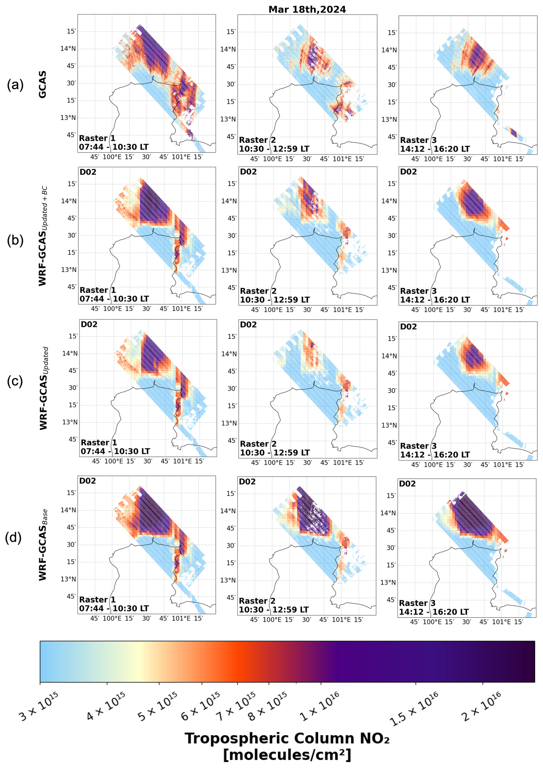
Figure 8 Spatial comparison over the BMR on 18 March 2024 of tropospheric NO₂ columns from (a) GCAS, (b) WRF-GCAS_Updated+BC D02, (c) WRF-GCAS_Updated D02 and (d) WRF-GCAS_Base D02 for raster periods corresponding to morning, afternoon, and early evening local time.

3.5 Selection of the inversion method

To identify the optimal inversion method to be used for model correction, we test which method can successfully recover WRF-Chem's prior daytime NO_x emission profile. To do so, we apply the ddeq inversion algorithms to WRF_Base, to produce “top-down” estimates from the model, which we will refer to as model-derived emissions. To replicate the satellite output, we re-gridded the model output from its native resolution to the satellite swath grid using the Universal Regridder for Geospatial Data (xESMF) Python package (Zhuang et al., 2025). A nearest-neighbor interpolation scheme was used to preserve spatial gradients and align the model resolution to that of the satellite observations. This spatial re-gridding was performed on an hourly basis, corresponding to the nearest observation time (00:45–06:45 UTC). Following re-gridding, model NO₂ mixing ratios were vertically interpolated to the satellite pressure levels using a one-dimensional linear interpolation to ensure consistency between the model and observed data for averaging kernel application. After interpolating model output to GEMS's spatial and pressure grid, we computed the model's tropospheric column NO₂ (molecules cm⁻²). This is done by converting the model's standard output of NO₂ volume mixing ratio (ppmV) to a number density with the ideal gas law:

$$\begin{array}{}\text{(9)}& {\mathrm{NO}}_{{\mathrm{2}}_{\mathrm{Number}\mathrm{Density}}}={\displaystyle \frac{P\cdot {\mathit{\chi }}_{{\mathrm{NO}}_{\mathrm{2}}}\cdot N_{\mathrm{A}}}{R\cdot T}}\end{array}$$

where ${\mathit{\chi }}_{{\mathrm{NO}}_{\mathrm{2}}}$ is the NO₂ mixing ratio in ppmV, P is pressure in Pa, T is temperature in K, R is the gas constant (8.314 J mol⁻¹ K⁻¹), and N_A is Avogadro's number (6.022×10²³ mol⁻¹). The number density is then multiplied by the thickness of each vertical model layer Δz to obtain the NO₂ amount per unit area. Summing across all layers yields the total column NO₂:

$$\begin{array}{}\text{(10)}& \begin{array}{rl}{\mathrm{NO}}_{\mathrm{2}{}_{\mathrm{WRF}-\mathrm{GEMS}}}=& {\displaystyle \frac{\mathrm{1}}{\mathrm{10}{}^{\mathrm{4}}}}\times \sum \underset{k}{}\\ & \left(A_k\cdot {\mathrm{NO}}_{{\mathrm{2}}_{\mathrm{Number}\mathrm{Density},k}}\cdot \mathrm{\Delta }z{}_k\right)\end{array}\end{array}$$

where A_k is the averaging kernel value at layer k, Δz_k is the thickness of the model layer k, in meters, and $\frac{\mathrm{1}}{{\mathrm{10}}^{\mathrm{4}}}$ converts the units to molecules cm⁻². As WRF-Chem has no stratosphere, we regard this as the tropospheric column NO₂. The satellite averaging kernel weights each model layer based on how sensitive GEMS is to that part of the atmosphere. This allows for a direct comparison with GEMS retrievals.

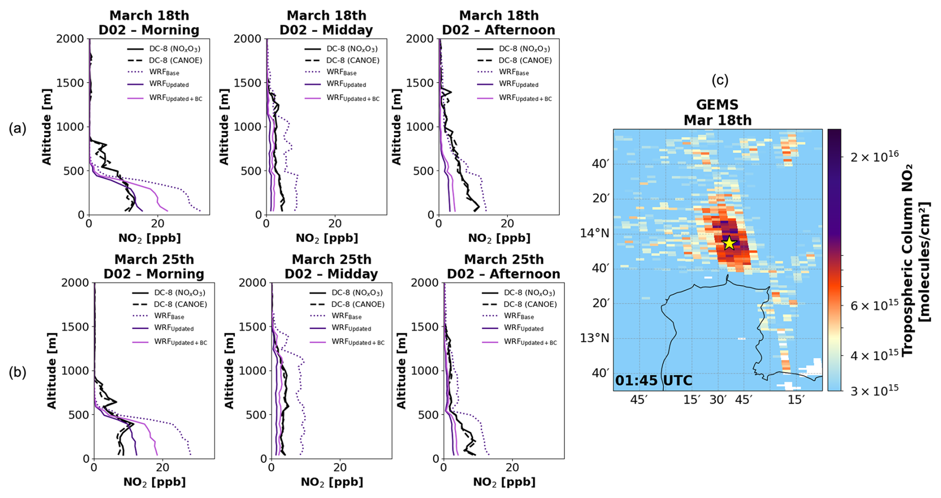
Figure 9 Comparison of WRF-Chem D02 simulations (WRF_Base: dotted dark purple; WRF_Updated: solid dark purple; WRF_Updated+BC: solid magenta) with airborne in situ measurements from the CANOE (dashed black) and NO_xO₃ (solid black) instruments aboard the DC-8 for (a) 18 March and (b) 25 March 2024. Profiles are grouped by morning (06:00–11:00 LT), midday (11:00–13:00 LT), and afternoon (13:00–17:00 LT) approaches at Don Mueang International Airport in northern Bangkok, whose location relative to the Bangkok urban plume is shown within a GEMS snapshot in (c).

We compute model-derived NO_x emissions from re-gridded WRF_Base (which we denote as WRF-GEMS) with ddeq and the resulting average daytime profile for Bangkok is illustrated in Fig. 3c. The shape and magnitude of model-derived NO_x emissions differ substantially from the satellite-derived emission data. Model-derived emissions are initially >50 % larger than GEMS-derived emissions. Additionally, there are minimal changes in the daytime pattern present in any of the inversion methods. In fact, WRF-GEMS D02 sees an increase in emission between 08:00 and 10:00 LT, a pattern that disagrees with the observed satellite-derived emissions. The results here further illustrate the need for an hourly correction to the model's emission profile, rather than applying a single scaling factor across all hours. The WRF_Base prior emission profile is shown by the black dashed line. For this comparison, we smoothed the prior emission profile using a 3 h backward-looking average to account for the accumulation and chemical evolution represented implicitly in the inversion results. Overlaying the prior emissions shows that the model-derived CSF method most accurately recovers them, likely due to its use of downwind fluxes and multiple cross-sections across the plume, which provide additional constraints on plume evolution and reduce sensitivity to local errors in wind fields, plume definition, and missing data compared to the IME and GP methods. As a result, we select the CSF inversion method moving forward to correct and scale WRF-Chem's daytime NO_x emission profile.

4 Model emission adjustment framework

To better represent NO_x emissions over Bangkok, we developed an optimization framework to re-scale and shape WRF-Chem's prior daytime emissions across the BMR (see step 2, Fig. 2). The prior emissions come from monthly EDGAR v5 values. The optimization uses a cost function J(x) to adjust daytime prior emissions based on GEMS NO_x retrievals, incorporating the lifetime and uncertainties from both the model and observations.

4.1 Optimization of daytime anthropogenic NO_x emissions

4.1.1 Observational constraint

The GEMS average daytime NO_x profile (blue lines in Fig. 3a, b) from the CSF method provides the observational constraint. Two versions of the optimization are performed: one using the constraint derived from the bias-corrected retrievals, and one without it. To improve consistency between the observed and modeled columns, we applied a correction factor to the constraint to account for the portion of the NO₂ column that GEMS does not capture because of reduced sensitivity near the surface. Although the air mass factor (AMF) calculation includes vertical weighting, the retrieved GEMS column can still underestimate tropospheric NO₂ in conditions where a substantial fraction resides in the lowest few hundred meters and is weakly sensed by the instrument. To address this sensitivity, satellite-derived NO_x emission estimates were scaled using the ratio of model-derived emissions obtained from the full column (i.e., Eq. (10) excluding the A_k) and from the same column after application of the GEMS averaging kernel:

$$\begin{array}{}\text{(11)}& \mathit{y}=e_{\mathrm{GEMS}}\times \left({\displaystyle \frac{e_{\mathrm{WRF}{}^{\mathrm{TC}}}}{e_{\mathrm{WRF}{}^{\mathrm{AK}}}}}\right)\end{array}$$

where e_GEMS, $e_{{\mathrm{WRF}}^{\mathrm{TC}}}$, and $e_{{\mathrm{WRF}}^{\mathrm{AK}}}$ denote the satellite-derived daytime NO_x emission profiles derived from GEMS, model-derived emissions from WRF-Chem (D02) total columns, and model-derived emissions from the same columns after applying the GEMS averaging kernel, respectively. Hourly correction factors ranged between 1.05 and 1.33, where larger corrections (e.g., 1.33) were present in the morning hours, 01:00–02:00 UTC. This vertically adjusted satellite-derived emission vector was used as the observational constraint, y in the optimization.

4.1.2 Prior assumptions, lifetimes, and temporal weighting

The prior for the optimization, x_b, refers to the bottom-up daytime NO_x emission profile shown in the black dashed line in Fig. 3c. For the optimization, it is necessary to map the prior emissions to the satellite-derived emissions through the observational operator H. Satellite emissions of NO_x represent not only emissions from the current hour, but also contributions from preceding hours. To address this, we introduce an operator H that links the prior daytime hourly emissions to the satellite-derived NO_x amounts. Each row of H defines how emissions from a set of prior model hours contribute to an observation at time, t_i.

For each GEMS observation hour t_i, we assume that the column enhancement is influenced by emissions from a backward-looking window of 3 model hours: $t_i-\mathrm{2},t_i-\mathrm{1},t_i$.

The window choice was determined by comparing inversion results to model priors using averaging windows from 1 to 6 h. The 3 h window provided the best agreement with the model-derived CSF emissions as shown in Fig. 3c. Within this window, the contribution from each prior hour depends on the atmospheric lifetime of NO₂ for that hour. We use hourly lifetimes, τ, derived from the GEMS-based CSF inversion in Eq. (7), where τ is fitted from observed along-plume decay using ERA5 winds, and is therefore independent of WRF-Chem meteorology. This ensures the satellite-derived emission estimates are completely independent of the WRF-Chem simulations. For reference, WRF-Chem-derived decay times are generally longer than those inferred from GEMS, reflecting differences in modeled vs. observed loss and dilution processes. Hours with no satellite information, are assigned a default lifetime of 3 h. We then apply a simple exponential decay law:

$$\begin{array}{}\text{(12)}& w\left(\mathrm{\Delta }t\right)=\exp \left(-{\displaystyle \frac{\mathrm{\Delta }t}{\mathit{\tau }}}\right)\end{array}$$

where: $\mathrm{\Delta }t\mathit{ϵ}\mathit{\{}\mathrm{0},\mathrm{1},\mathrm{2}\mathit{\}}$ is the time lag between when NO_x was emitted and when its NO₂ enhancement is observed. These raw weights are normalized within each row of H to ensure mass conservation:

$$\begin{array}{}\text{(13)}& {\mathbf{\text{H}}}_{i,j}={\displaystyle \frac{w\left(\mathrm{\Delta }{t}_j\right)}{{\sum }_{j^{\prime }}w\left(\mathrm{\Delta }{t}_{j^{\prime }}\right)}}\end{array}$$

Thus, H_i,j, represents the fraction of the observed column at hour i, that is attributable to emissions from model hour j. This framework of H ensures that shorter lifetimes contribute to a stronger emphasis on the most recent emissions, appropriately reflecting rapid chemical loss, and longer lifetimes spread the influence of emissions over multiple hours, consistent with slower decay. By embedding this chemical persistence into the operator, H, we obtain a physically representative mapping between model emissions and the satellite observations that are used to constrain them.

4.1.3 Solution for posterior daytime emissions

A model corrected daytime NO_x emission profile (posterior), $\widehat{\mathit{x}}$ was obtained by minimizing the following cost function:

$$\begin{array}{}\text{(14)}& \begin{array}{rl}J\left(\mathit{x}\right)& ={\displaystyle \frac{\mathrm{1}}{\mathrm{2}}}{\left(\mathit{y}-\mathbf{H}\mathit{x}\right)}^T{R}^{-\mathrm{1}}\left(\mathit{y}-\mathbf{H}\mathit{x}\right)\\ & +{\displaystyle \frac{\mathrm{1}}{\mathrm{2}}}{\left(\mathit{x}-{\mathit{x}}_{\mathrm{b}}\right)}^T{B}^{-\mathrm{1}}(\mathit{x}-{\mathit{x}}_{\mathrm{b}})\end{array}\end{array}$$

where y is the satellite-derived, column-corrected NO_x emission vector, x is the unknown corrected model daytime emission profile, x_b is the model prior profile, $R={\mathit{\sigma }}_I{}^{\mathrm{2}}I,B={\mathit{\sigma }}_{\mathrm{B}}{}^{\mathrm{2}}I$ are the observation and background error covariance matrices, and H is the observational operator matrix described above. In this study, we use R= 1 and B= 10. These values were based on sensitivity tests in which we vary R and B over several orders of magnitude. The chosen values represent a compromise that allowed the posterior emission profile to closely follow the satellite constrains while preventing excessive deviations from the prior emission profile. To account for temporal correlation in prior emission errors, the elements of B are defined as:

$$\begin{array}{}\text{(15)}& B_{i,j}={\mathit{\sigma }}^{\mathrm{2}}{}_B\exp \left(-{\displaystyle \frac{\mathrm{|}{t}_i-t_j\mathrm{|}}{L}}\right)\end{array}$$

where |t_i−t_j| is the temporal separation between emission hours i and j, and L is the temporal correlation length, set to L= 2 h in this study. This setup ensures that prior errors vary smoothly in time rather than independently hour-to-hour. Finally, the cost function was minimized using a Sequential Least Squares Quadratic Programming (SLSQP) algorithm – minimize(method=“SLSQP”), v1.16.2 (SciPy Developers, 2025; Nocedal and Wright, 2006). The result is a corrected model hourly emission vector, $\widehat{\mathit{x}}$, that balances the satellite-derived emissions with the model's prior estimate while accounting for chemistry and transport behavior (Fig. 4).

Figure 4a and c illustrate the raw hourly daytime NO_x for both the prior model (dashed purple) and the optimized version (solid purple), based on constraints applied without and with the GEMS bias correction, respectively. In both bases, the posterior profile departs notably from the prior in both magnitude and shape. In the case without the bias-corrected constraint (Fig. 4a), a morning peak is visible at 07:00 LT, followed by a steady decline until 13:00 LT. This pattern is consistent with temporal patterns in weekday traffic intensity in Bangkok found in Ly et al. (2015), which found the morning traffic to peak at 07:30 LT ending at 09:30 LT, and the evening peak from 17:00 to 20:00 LT (outside of GEMS observing window). Activity begins to increase at 13:00 LT which corresponds to the NO_x increase we begin to see in the posterior result after 06:00 UTC. The case with the bias-corrected constraint (Fig. 4c) places peak morning emission closer to the model prior at 07:00–08:00 LT, with NO_x declining slightly later, at 09:00 LT. NO_x emission begins to increase after 13:00 LT similar to what is depicted in Fig. 4a. When the prior and posterior hourly emissions are passed through H, we obtain a temporally smoothed emission profile consistent with what GEMS would observe (Fig. 4b, d). Figures 4b and d show the posterior profile closely reproduces the GEMS-derived daytime pattern, indicating the optimization effectively aligns model emissions with satellite-derived emissions while preserving components of the prior model behavior.

4.2 Adjustment of WRF-Chem diurnal emission profiles

Using satellite-derived NO_x emissions and the posterior results above, we correct the WRF-Chem 24 h input emissions over the BMR. Since GEMS provides estimates over 01:00–07:00 UTC, we only have posterior model emissions over this window. To apply these updates to the full gridded 24 h WRF-Chem anthropogenic emission input (00:00–23:00 UTC), while preserving the model's spatial distribution, we compute hourly scaling factors which we use to adjust the gridded prior NO_x emissions. Because GEMS provides constraints only during the daytime overpass window, the derived scaling below primarily reflects daytime emission adjustments. We therefore apply the mean scaling factor uniformly during the nighttime hours to preserve the prior temporal structure and avoid introducing artificial discontinuities between the constrained and unconstrained hours, particularly given the large daytime emission reductions. This approach is consistent with previous satellite-constrained emission studies (e.g., Goldberg et al., 2019) which constrain emission magnitude based on a single daytime value derived from OMI. Where available, locally derived temporal profiles should be used to better represent regional emission patterns; in this study, our prior profile reflects the best available regional representation for Asia at the time of study.

To compute the factors, hourly WRF-Chem NO and NO₂ prior emission fields were summed across the vertical levels and masked to the Bangkok region bounded by N–S: 13.5–15.0°, W–E: 100.2–100.9°, using the WRF-Chem grid. In WRF-Chem, NO_x emissions are stored as NO₂-equivalent mass (“NO_x as NO₂”), so all conversions use the molecular weight of NO₂. The total emissions were converted to mol h⁻¹ using a molecular weight of 46.01 g mol⁻¹ and an area of 16 km² per grid cell (following the resolution of D02). Each posterior emission, ${\widehat{\mathit{x}}}_h$ was converted from kg s⁻¹ to mol h⁻¹ and divided by the corresponding original WRF-Chem total to compute a scale factor, f for each hour h:

$$\begin{array}{}\text{(16)}& f={\displaystyle \frac{{\widehat{\mathit{x}}}_{\mathrm{h}}\times \frac{\mathrm{1000}}{\mathrm{46.01}}\times \mathrm{3600}}{E_H^{\mathrm{WRF}}}}\end{array}$$

where $E_H^{\mathrm{WRF}}$ is the original domain-integrated prior NO_x emissions for hour h. Since the optimization covered hours with GEMS measurements, the scaling factors for the remaining model hours were computed using the ratio of average daytime posterior emissions where averages are taken over the constrained hours. Finally, we apply the scaling factors spatially over the BMR. The scaling factor was applied to the hourly WRF-Chem anthropogenic emissions prior files and only to NO and NO₂ grid cells within the BMR mask. This preserves the original spatial distribution but adjusts the total prior emissions to match the posterior values. The updated emission files were then used to initialize an updated model simulation, ran for the ASIA-AQ deployment period, which we will refer to as WRF_Updated (see step 3, Fig. 2).

Figure 4e compares the average diurnal prior profile over BMR with the updated profile derived from the optimization and scaling procedure. The optimized diurnal profile based on the bias-corrected GEMS constraint is illustrated by the light pink line. The updated profiles show a notable increase in NO_x between 07:00 and 10:00 UTC (14:00 to 17:00 LT), which may reflect the beginning of a rush-hour signal over the city. Nighttime emissions retain the overall shape of the prior profile but are scaled downward based on the daytime average. Figure S6 maps the spatial distribution of these updates across BMR, showing the largest differences in the late afternoon and early evening, with localized reductions of up to 400 mol km⁻² h⁻¹ in the updated input emissions.

4.3 Comparison with bottom-up emission inventories

To place the updated NO_x emissions in context of existing emission inventories, we compared total monthly emissions over the BMR against several widely used bottom-up inventories, our top-down emissions (including bias-corrected results – This Study_BC), and emissions from a chemical reanalysis product (Fig. 5). These include HTAP v3.2 (base 2019), a local Thailand Inventory (THAI-KMUTT) (base 2019), MIX v2.3 (base 2017), EDGAR v5 (base 2015), CEDS (base 2024), our study (2024), and the Tropospheric Chemistry Reanalysis (TCR-3) top-down emissions TCR-3 (2024) (Miyazaki et al., 2020). Across inventories, monthly totals for March can vary nearly by an order of magnitude, highlighting large uncertainty in regional NO_x sources and emissions processing methodology. For example, although both HTAP v3.2 and MIX v2.3 rely on the REAS framework (Kurokawa and Ohara, 2020) for Asian anthropogenic emissions, they are derived from different REAS versions, temporal coverage, and processing assumptions, which can lead to substantial differences in absolute emission magnitudes over Bangkok. HTAP v3.2 is based on REAS v3.2.1, which provides monthly emissions for 2000–2015 at a spatial resolution of 0.25°. In the HTAP product, these emissions are re-gridded to 0.1° by assuming a uniform spatial distribution within each grid cell (Guizzardi et al., 2025). In contrast, the MIX inventory is based on REAS v2, which covers 2000–2008 and reflects earlier emission estimates and activity data (Li et al., 2024). REAS v2 was subsequently extended to 2010 following the scaling approach described by Kurokawa and Ohara (2020).

Overall, HTAP v3.2 depicts the highest NO_x totals at 31 kt month⁻¹. THAI-KMUTT follows with emissions at ∼ 20 kt month⁻¹, reflecting its incorporation of detailed regional activity from local emissions data. The coarser-resolution MIX v2.3, and EDGAR v5, and CEDS inventories reflect lower totals, at ∼ 13, 11, 10 kt month⁻¹ respectively, consistent with the use of different emission estimation methodology and older base years for MIX and EDGAR which correspond to lower macro-economic (e.g., GDP) indicators in Thailand compared to 2019. Lastly, GEMS top-down NO_x estimates (including bias-corrected results) and TCR-3 estimates based on the chemical reanalysis using TROPOMI NO₂ indicate substantially lower emissions (2–4 kt month⁻¹). These reduced magnitudes may result from both recent emission declines and structural differences in how emissions are computed (i.e., top-down perspective).

It is important to note uncertainties are present and differ amongst emission methods. For example, bottom-up inventories depend on activity data, emission factors, spatial approximations, and assumptions that may not capture rapid socio-economic changes or region-specific behavior. Top-down estimates incorporate uncertainties from their respective satellite retrievals, reanalysis data (e.g., ERA5), averaging kernels, chemical lifetime assumptions, and forecast-model transport and chemistry (e.g., TCR-3). Together, these differences highlight the value of combining observational constraints with updated bottom-up information to define NO_x emission estimates.

5 Evaluation against satellite observations

To evaluate the performance of WRF-Chem (Base + Updated) NO₂ simulations during the ASIA-AQ period (14–27 March 2024) in Bangkok, we first compared model output with satellite tropospheric column NO₂ retrievals from GEMS v3 data. For GEMS observations, pixels were filtered based on cloud fraction (CF < 0.3). The GEMS averaging kernel and air mass factor data were used to isolate tropospheric contributions and account for satellite instrument sensitivity. To enable a direct comparison with our model output, we re-gridded model output from its native resolution to the satellite swath grid as explained in Sect. 3.3. As before, we refer to the re-gridded model simulations with the GEMS averaging kernel applied as WRF-GEMS. To evaluate regional NO₂ variability, we aggregated satellite and model-derived tropospheric column NO₂ values over the BMR, by defining a N–S (13.5–14° N), W–E (100.3–100.9° E) bounding box for the area. For pixels within this boxed region, we calculate the mean NO₂ concentration, minimum NO₂, maximum NO₂, standard deviation, and the 10th and 90th percentiles to characterize regional variability. This analysis was repeated on an hourly basis for each co-located WRF-Chem and GEMS dataset, providing a regionally aggregated view of column NO₂ for intercomparison.

The results shown here are based on satellite comparisons using the non-bias corrected model results and are intended to illustrate that the optimization brings the model closer to GEMS observations. The maps shown in Fig. 6 illustrate a spatial comparison of (a) GEMS, (b) updated model results, WRF-GEMS_Updated D02, and (c) base model, WRF-GEMS_Base D02 tropospheric columns NO₂ over the BMR for several snapshots on 18 March 2024. Results for D01 can be found in Figs. S6 and S7. GEMS generally places BMR city enhancements between 5×10¹⁵ and 2×10¹⁶ molecules cm⁻² in a N–S direction. Both WRF_Updated D01, D02 generally reflect the spatial distribution and magnitude of tropospheric column NO₂ observed during daylight hours. WRF_Updated D02 (Fig. 6b) tends to place the city plume more northward at 04:00 and 07:00 UTC compared to what is observed in GEMS data (Fig. 6a). This spatial discrepancy is likely related to overpredicted model winds (further discussed in Sect. 6.1) which displaces the plume in a northward direction. Additionally, while the inversion framework adjusts emission magnitudes temporally, it does not correct spatial errors in plume transport or source distribution (See Sect. 7.2 for further discussion). Nevertheless, the daytime pattern seen in GEMS is accurately reflected in WRF_Updated with column NO₂ values at their peak in the morning hours (08:00 LT), decreasing substantially throughout the afternoon (14:00 LT) due to photochemical interactions. This is a substantial improvement from WRF_Base, which sees a large overestimation of NO₂ in the morning hours followed by persistent and growing NO₂ columns throughout the afternoon as seen in Fig. 6c.

The time series in Fig. 6d illustrates a full comparison of daytime tropospheric column NO₂ values across model types in D02 (see Fig. S7 for D01) for the duration of ASIA-AQ. WRF-GEMS_Updated indicates a clear reduction in error and bias from WRF_Base as illustrated by the reduced NO₂ columns and model spread. WRF_Updated also indicates corrected daytime patterns compared to WRF_Base, indicating better consistency with GEMS observations for the deployment period with few exceptions such as 22 March where GEMS has peaks in the afternoon (further discussed in Sect. 6.1).

6 Evaluation using independent observations

To independently assess the performance of the optimized WRF-Chem simulations, we compared three model configurations: WRF_Base, WRF_Updated, and WRF_Updated+BC for D01 and D02 against a suite of independent airborne and ground-based observations distinct from the satellite measurements used in the emission optimization process (see step 4, Fig. 2). Comparisons between WRF_Updated and WRF_Updated+BC reflect the sensitivity of the model results to biases in the GEMS retrieval used to constrain emissions in the optimization process. This evaluation primarily emphasizes the results of D02 (4 km), which more directly represents urban-scale processes and exhibits improved performance compared to D01 across multiple observational datasets. These datasets provide an unbiased test of how well the model reproduces meteorological conditions and trace gas amounts beyond those directly constrained from GEMS observations. By evaluating WRF-Chem against surface monitoring networks (Thailand PCD), Pandora spectrometer measurements, and airborne ASIA-AQ data (e.g., GCAS NO₂ columns, DC-8 vertical profiles), we examine the model's ability to capture daytime variability, vertical structure, and surface concentrations of NO₂ across different spatial and temporal scales. Evaluation amongst these diverse datasets, therefore, helps to support the robustness of the emission correction framework described in this paper.

6.1 Meteorological evaluation: winds and PBL height

6.1.1 Evaluation methodology

To assess the performance of WRF-Chem meteorological fields, modeled wind speed and direction were evaluated against surface observations across the BMR during the ASIA-AQ campaign, 14–27 March 2024. Biomass burning was active in the region during the study period, particularly over northern Thailand and Myanmar, with peak activity occurring in mid-March. However, transport to Bangkok was likely limited due to weak synoptic flow and short chemical lifetime of NO_x, reducing its impact on urban concentrations of NO_x in the BMR. Following 20 March, precipitation suppressed fire activity, further minimizing its impact. While biomass burning may contribute to broader regional enhancements, its impact on the inversion results and coincident model evaluation over Bangkok is expected to be minor.

Surface observations of wind speed (m s⁻¹) and direction are obtained from Thailand Pollution Control Department (PCD) ground monitor network data. Hourly surface wind observations from PCD network data were co-located with corresponding model outputs for D01 and D02. For each site, model data were extracted from the nearest grid cell and interpolated to observation timestamps. Daily wind roses were constructed to visualize and compare the frequency distribution of wind speed and direction between the model and observations. For each station, wind speeds were binned into intervals of 0–1, 1–3, 3–5, and 5–8 m s⁻¹ and wind directions were grouped into 16 compass sectors. Normalized frequency counts were computed to highlight dominant flow patterns. Data was averaged across stations within a larger bounding box around BMR, N–S (12.5–15° N), W–E (99.5–101.5° E). For meteorology, we use a large box that spans the regional flow influencing Bangkok so that we capture plume transport into and out of the city. Figure S8a illustrates the station locations and averaging domains in Bangkok.

Additionally, we performed an evaluation of planetary boundary layer height (PBLH) to gauge the model's ability to capture daily PBLH magnitude and development during the deployment period. Observed PBLHs were derived from the NASA Langley airborne High Spectral Resolution Lidar Generation -2 (HSRL-2) data following a machine learning approach described in Christopoulos et al. (2025) for ASIA-AQ flight days, 18 March, 19 March, 23 March, and 25 March 2024. We evaluate PBLHs for aircraft raster periods (i.e., Raster 1: morning, Raster 2: afternoon, Raster 3: late afternoon/evening hours) and co-locate the observed PBLHs to modeled PBLHs based on a nearest grid-cell approximation.

6.1.2 Model-observation wind discrepancies

Within the observational data, a pronounced synoptic transition occurred over Thailand on 20–21 March 2024, during which winds reversed from the typical southwesterlies that were present during the deployment period to northeasterlies, weakened substantially, coinciding with a drop in PBLH, and increased atmospheric stability (see observations; Figs. S9, S10). This transition played a major role in PM_2.5 and ozone exceedances by promoting stagnation over the BMR. The WRF-Chem simulation failed to capture the timing or strength of this abrupt wind shift and associated stagnation (Figs. S2a, b and S9b, c). The model instead maintained stronger southwesterly flow and higher PBLH, which led to unrealistic vertical mixing patterns compared to the observations (Figs. S9, S10). Since this mismatch drives discrepancies between model and observations that are unrelated to emissions adjustments/inversions, we exclude 20–21 March from the inversion/air quality evaluation. Although the simulation is driven by FNL, it is possible for WRF-Chem to mis-time a rapid synoptic transition. This event evolved on a relatively short spatial and temporal scale, and the coarse FNL boundary conditions may not have fully resolved the sharp changes in low-level flow. In addition, local processes (i.e., convection, PBL mixing, land-sea interactions) around Bangkok can cause the model to drift from the observed timing once it is integrated forward. We suspect these factors likely contributed to the later wind shift in WRF-Chem. We additionally found WRF-Chem (D01, D02) systematically overpredicts wind speed throughout the deployment (Fig. S2a, b; Table S2) with better agreement from the high-resolution 4 km domain. This bias likely arises from the fact that many PCD monitors are embedded within the complex urban environment of Bangkok, which are not fully resolved at WRF-Chem's spatial scale.

The consequences of this mis-timed synoptic transition are most pronounced on 21 March as demonstrated in the next section, when weak large-scale flow made the simulation highly sensitive to local processes. Under these conditions, WRF-Chem misses the stagnation and dilutes pollutants too quickly. This helps explain why the model performs worst during the highest observed PM_2.5 and O₃ episode. These results indicate that forecast performance during similar weak-flow pollution events would benefit from improved representation of urban boundary-layer processes (e.g., surface roughness, urban canopy effects, and land–sea breeze structure).

6.1.3 Model-observation PBLH discrepancies

As shown in Fig. S10 and summarized in Table S3, WRF-Chem generally captures the temporal evolution of the PBLH observed by the aircraft. During the daytime (afternoon hours represented by Raster 2–3), the simulated PBL is broadly comparable to the observations, with median values that are often similar. However, the magnitude and sign of the model bias vary by day, with WRF-Chem demonstrating both over- and under-estimation likely related to the meteorological conditions. This day-to-day variability suggests PBLH biases are not systematic during the afternoon and may influence surface pollution dilation differently across individual cases, potentially contributing to variability in simulated daytime NO₂ concentrations rather than a consistent model bias.

6.2 Surface air quality evaluation

To evaluate model performance of surface trace gases, modeled surface mixing ratios of NO₂, NO_x, and O₃ were evaluated against observations across BMR during 14–27 March 2024. Surface observations of these constituents (in ppbV) were obtained from Thailand PCD ground monitor network data. Like the evaluation of wind speeds and direction, data was co-located by extracting model information from the nearest grid cell and matched to the observation timesteps. Station data and model data were averaged across stations located within the Bangkok urban plume, bounded by N–S (13.5–14.6° N), W–E (100.2–101° E). Figure S8b illustrates the station locations and averaging domain in Bangkok. For the air quality evaluation, we restrict the station averaging domain to a smaller area over the Bangkok urban plume. This smaller domain allows us to assess how the inversion and optimization specifically correct the local plume structure as opposed to a broader regional background.

6.2.1 NO₂ and NO_x

Figure 7a, b, and c shows a comparison of average surface NO₂, NO_x, and O₃ (ppbV) for stations located within the Bangkok urban plume during the ASIA-AQ deployment for D02. D01 results are available in Fig. S11. The 20–21 March is shaded in grey to indicate the period where the model mis-represented synoptic conditions resulting in enhancements in the observed concentrations due to stagnation. During this time, NO₂ and NO_x reached as high as 49, and 59 ppbV, respectively. O₃ peaked at 103 ppbV the following day, on 22 March. Excluding this event, observed NO₂ and NO_x for this period generally ranged between 3–17 ppbV, and 3.5–22 ppbV respectively. Overall, there is a clear improvement in the representation of NO₂ and NO_x during this period in WRF_Updated and WRF_Updated+BC as shown in Fig. 7a and b.

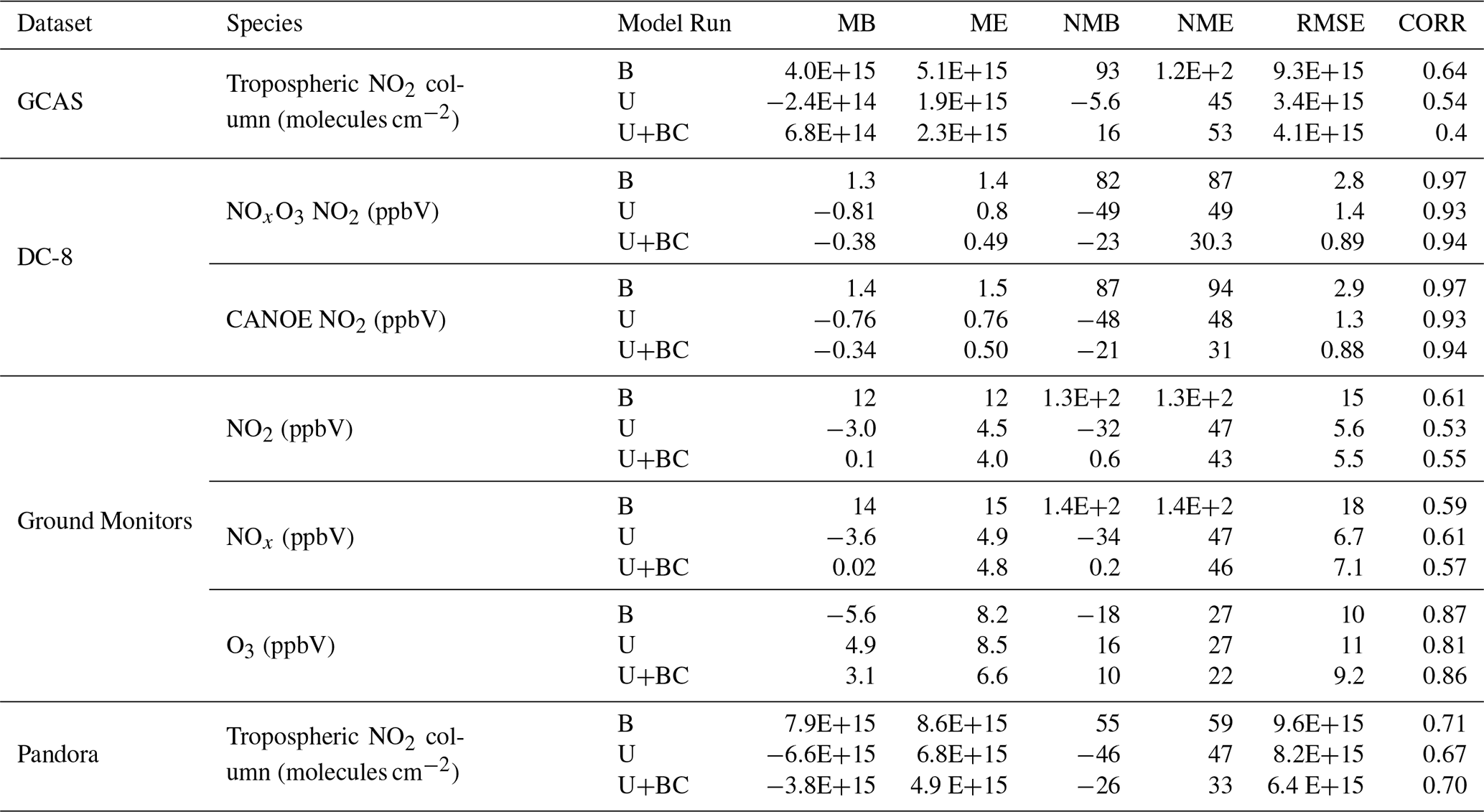
Table 2 depicts summary statistics for this analysis. The baseline simulation, WRF_Base overestimates both NO₂ and NO_x with mean biases of +12 and +14 ppbV, respectively. With updated emissions, these large positive biases in WRF_Updated were eliminated and reversed, yielding mean biases of −3.0 ppbV for NO₂ and −3.6 ppbV for NO_x. The remaining negative bias is likely linked to the overprediction of winds, associated advection, and inversion related biases, which leads to locally diluted concentrations near urban sites as shown in the previous analyses. WRF_Updated+BC further reduces the residual bias related to WRF_Updated, bringing mean biases closer to zero (e.g., +0.1 ppbV for NO₂ and +0.02 ppbV for NO_x), while maintaining comparable error and correlation, indicating accounting for the GEMS retrieval bias prior to inversion provides a modest additional improvement in model performance. Correlations with observed NO₂ and NO_x remain moderate (r= 0.5–0.6) reflecting potential spatial discrepancies in WRF_Updated as seen in the previous analyses. Average diurnal cycles of NO_x for D02, D01 are further illustrated in Fig. S12a and c. Observed NO_x shows a clear morning peak and lower midday concentrations driven by boundary layer evolution. WRF_Base overestimates NO_x and exaggerates the morning peak while WRF_Updated (dark purple) substantially improves both magnitude and timing but underestimates the evening peak values. WRF_Updated+BC shows mixed performance with an overprediction of the morning peak while the evening peak aligns more closely with observations compared to WRF_Updated, indicating a trade-off in how the bias correction might redistribute NO_x across the diurnal cycle in the updated models.

Table 2 Summary of WRF-Chem D02 validation statistics for WRF_Base (B), WRF_Updated (U), and WRF_Updated+BC (U+BC) simulations evaluated against independent observational datasets. Metrics include mean bias (MB), mean error (ME), normalized mean bias (NMB), normalized mean error (NME), root-mean-square error (RMSE), and Pearson correlation coefficient (CORR).

6.2.2 O₃

Observed O₃ generally ranged between 14 and 57 ppbV, excluding the stagnation event on 20–21 March, and the baseline model captures this range reasonably well (Fig. 7c). After updating the emissions, O₃ increases in WRF_Updated and WRF_Updated+BC primarily at night, consistent with reduced NO titration following the decrease in NO_x emissions. Average diurnal cycles in D02 (Fig. S12b, d) show that daytime O₃ production changes only modestly between base and updated simulations, indicating the emission update mainly affects nighttime chemistry, as opposed to shifting photochemical O₃ formation in the daytime. This pattern is reflected in the change in overall mean bias in Table 2, which shifts from an underprediction (−5.6 ppbV) to an overprediction (+4.9 ppbV) in WRF_Updated. The overprediction is not as substantial in WRF_Updated+BC (+3.1 ppbV). While WRF_Updated exhibits an earlier O₃ peak in D02 compared to observations, this shift is not present in D01 despite the same emission inversion being applied. This likely suggests the discrepancy is driven by domain-dependent differences in meteorological or chemical processes, rather than an error in the inferred NO_x emission timing. The O₃ peak is better represented in WRF_Updated+BC.

The relatively weak daytime O₃ response to decreased NO_x emissions is consistent with recent analyses of O₃ formation sensitivity during ASIA-AQ with in situ measurements, which indicate that the BMR exhibits mixed sensitivity to NO_x and VOCs, in contrast to the predominantly NO_x-limited regimes observed at other ASIA-AQ locations (e.g., Manila) (Cho et al., 2026). In this mixed-sensitivity regime, changes in NO_x emissions alone are not expected to strongly perturb daytime O₃ production, further providing validation for the minimal daytime O₃ response observed here. The magnitude of the daytime O₃ response varies by domain/model as shown by the D01 results (Fig. S12d). Although WRF_Updated D01 better matches observed daytime O₃, this apparent improvement likely reflects NO_x titration associated with spatial dilution.

Overall, these results suggest that while the updated emissions improve the model's NO_x representation, further improvements in VOC representation and local mixing processes may be needed to fully capture daytime O₃ levels in the BMR. Nevertheless, the updated emissions substantially improve the model's simulation of surface NO₂ and NO_x, resulting in a more realistic overall representation of air quality in Bangkok.

6.3 Evaluation with Pandora column observations

We additionally evaluate modeled NO₂ columns against Pandora measurements for the Bangkok site. Pandora NO₂ evaluation used Level 2 direct-sun total column retrievals, filtered for high-quality measurements (quality flag =10), and averaged to hourly means. Tropospheric columns from Pandora were estimated by subtracting coincident or closest GEMS stratospheric NO₂ at the nearest satellite pixel. Model columns were sampled at the nearest grid cell to the Pandora site and temporally matched to observations.

Figure 7d depicts a comparison of WRF_Base (light purple triangles), WRF_Updated (dark purple squares), WRF_Updated+BC (magenta dots) and Pandora (pink stars), tropospheric NO₂ column measurements for days with high quality data. Throughout this period, Pandora measurements generally ranged between approximately 7×10¹⁵ to 3.5×10¹⁶ molecules cm⁻² and fit between WRF_Base which places columns higher (e.g., up to 5×10¹⁶ molecules cm⁻²), WRF_Updated+BC and WRF_Updated which places columns lower (e.g. 2×10¹⁵ molecules cm⁻²). Average statistics between model cases for this analysis are shown in Table 2. Biases are generally similar between model cases. WRF_Base overestimates column NO₂ as illustrated by the mean bias ($+\mathrm{7.9}\times {\mathrm{10}}^{\mathrm{15}}$ molecules cm⁻²) whereas emissions updates contribute to an underestimation ($-\mathrm{6.6}\times {\mathrm{10}}^{\mathrm{15}}$ molecules cm⁻²). However, there are some improvements in absolute error metrics with ME and RMSE decreasing by roughly 20 % and 12 % respectively, and NME dropping from 61 % to 48 %. The greatest bias improvements overall are seen in WRF_Updated+BC ($-\mathrm{3.8}\times {\mathrm{10}}^{\mathrm{15}}$ molecules cm⁻²). Figure S13 illustrates the spatial distribution of mean tropospheric model NO₂ bias for GEMS and Pandora during the time reflected in Fig. 7d. In the WRF_Base simulation, a strong positive bias is seen within and north of the Pandora site, indicating the overestimation of NO₂ columns (up to 2×10¹⁶ molecules cm⁻²) in the urban plume relative to GEMS. This pattern reiterates the point that the prior anthropogenic emissions (based on EDGAR v5) were too large with pollutant accumulation occurring downwind of Bangkok as a result. After applying the emission updates, the WRF_Updated simulation essentially eliminates this bias. The overall bias near the Pandora site becomes close to neutral or slightly negative, demonstrating the optimization effectively corrected the spatial overprediction. WRF_Updated+BC further reduces the residual negative bias relative to WRF_Updated with NMB improving from −46 % to −26 % and RMSE decreasing from 8.2×10¹⁵ to 6.4×10¹⁵ molecules cm⁻². This indicates that accounting for the GEMS retrieval bias in the initial optimization process partially corrects the remaining underestimation, although some spatial discrepancies persist dude to transport and plume placement error. Examples of daily biases for WRF_Base D01, D02, and WRF_Updated D01, D02 can be found in Figs. S14 and S15.

6.4 Evaluation with ASIA-AQ aircraft measurements

The Airborne and Satellite Investigation of Asian Air Quality (ASIA-AQ) was a NASA field campaign conducted in February–March 2024 to advance the understanding of urban and regional air quality across East and Southeast Asia. Targeting several megacities (e.g., Manila, Seoul, Bangkok, Chiang Mai), the campaign combined satellite observations, aircraft measurements, ground-based monitoring, and modeling approaches to characterize pollution sources and validate satellite retrievals. A main objective of ASIA-AQ was to evaluate the data from GEMS. Airborne observations were collected using the NASA DC-8 in situ and LaRC G-III remote sensing aircraft, with coordinated support from ground-based networks such as Pandora and AERONET. Additionally, chemical transport models (e.g., GEOS-Chem, GEOS-FP, MUSICA, WRF-Chem, WRF-CMAQ) played a key role in real-time flight planning and post-campaign interpretation.

6.4.1 GCAS

The GEOstationary Coastal and Air Pollution Events (GEO-CAPE) Airborne Simulator (GCAS) is an airborne UV-Vis spectrometer that was flown on the G-III aircraft during the ASIA-AQ campaign. GCAS was designed to simulate the spectral capabilities of TEMPO and GEMS, but with a much finer pixel resolution of approximately 250×560 m at flight altitude (Janz et al., 2019; Lee et al., 2024). GCAS uses a push-broom remote sensing technique and consists of two spectrometer channels: a UV-Vis channel (300–490 nm) optimized for air quality measurements, and a Vis-NIR channel (480–900 nm) for ocean color observations (Kowalewski and Janz, 2014; Lee et al., 2024). This work focuses on the NO₂ retrieval from spectra in the UV-Vis channel. Retrieval details and validation results can be found in Judd et al. (2020) but were previously found to be unbiased with uncertainties within ± 25 %. As in previous field campaigns, the aircraft executed a “lawnmower” flight pattern with parallel flight lines spaced 6.3 km apart, providing about 10 % overlap between flight lines assuming a flight altitude of 8534 m. This flight strategy, combined with the instrument's 45° field of view, allowed for the generation of gap-free NO₂ column maps up to three times per day, period referred to as a “raster”. Due to the short duration of each raster period (∼ 3 h), local meteorological conditions often influence the fine-scale structures observed in the GCAS NO₂ data (Goldberg et al., 2024). Here, we evaluate the WRF-Chem runs against GCAS for several flight days: 18, 19, 23, and 25 March 2024.

We perform the evaluation for each raster separately to isolate specific flight patterns and accurately evaluate spatial gradients in NO₂ between the model and observations. For each analysis, GCAS pixels corresponding to the flagged raster were retained for comparison. Additional filters were applied to remove poor-quality retrievals. We masked pixels with cloud or sun glint contamination based on a provided flag variable (cloud_glint_flag =1) and discarded retrievals with missing data or undefined AMFs. GCAS provides separate NO₂ vertical columns above and below the aircraft, as well as model-derived scattering weights, and AMFs for both portions. The above and below aircraft contributions can be approximated as the stratospheric and tropospheric contributions, respectively. For this evaluation, we focus exclusively on the NO₂ column below the aircraft or the tropospheric column NO₂, which is the portion most relevant to surface-level air quality and most comparable to our WRF-Chem results. We compute the below-aircraft averaging kernel, $A_i^{\mathrm{below}}$, as:

$$\begin{array}{}\text{(17)}& A_i{}^{\mathrm{below}}={\displaystyle \frac{{\mathrm{SW}}_i}{{\mathrm{AMF}}_{\mathrm{below}}}}\end{array}$$

Here, SW_i represents the scattering weight for layer i, representing the sensitivity of the measured radiance to NO₂ in that layer. This averaging kernel represents the satellite-equivalent vertical sensitivity to NO₂ below the aircraft and was used to weigh the WRF-Chem vertical profile.

WRF-Chem output including, NO₂ mixing ratio, pressure, temperature, and height were used to compute air density and convert volume mixing ratios to number densities as previously done in the GEMS evaluation. Each GCAS pixel was temporally matched to the nearest model output time (rounded to nearest hour) and spatially co-located by finding the nearest WRF-Chem grid cell. To isolate the portion of the model column below the aircraft, we filtered the model levels based on the aircraft altitude reported at each pixel. We compute the tropospheric column as shown in Eq. (10). To generate a model column that reflects the vertical sensitivity of the GCAS retrieval, we interpolate the WRF-Chem profile to the number of GCAS vertical layers (49), converted the mixing ratios to number density, and applied the GCAS averaging kernel to yield WRF-GCAS.

The maps in Fig. 8 illustrate a spatial comparison between (a) GCAS, (b) WRF-GCAS_Updated+BC D02, (c) WRF-GCAS_Updated D02, and (d) WRF-GCAS_Base D02 over BMR for a flight day on 18 March 2024. D01 spatial comparisons are available in Fig. S16. 18 March represents a typical example of local pollution dominating BMR with minimal influences from long-range pollution transport and biomass burning. The GCAS instrument generally places tropospheric column NO₂ values in BMR between 5×10¹⁵ and 2×10¹⁶ molecules cm⁻², with the largest enhancements observed in the city center, as also seen in the GEMS data (Fig. 7). A clear N–S plume is visible in the data, reflecting persistent southerly onshore flow from the Gulf of Thailand. This pattern coincides with the seasonal shift from the northeast to southwest monsoon. Overall, WRF-GCAS_Updated and WRF-GCAS_Updated+BC generally better capture the spatial differences and magnitudes of tropospheric column NO₂ in BMR for different raster periods compared to WRF-GCAS_Base. WRF_Updated+BC outperforms WRF_Updated in capturing NO₂ column enhancements, particularly during raster 2 (late morning–afternoon LT). GCAS also illustrates enhanced NO₂ columns southeast of Bangkok in a region known as the Eastern Economic Corridor (EEC), a major hub for industrial activity (e.g., automotive manufacturing, petrochemicals, electronics). WRF_Updated, WRF_Updated+BC, and WRF_Base tend to underestimate pollution levels in the EEC. This is likely related to wind speed overprediction and a lack of updated regional source data in the EDGAR v5 inventory (since this is a region outside of the performed inversion). Information from a local emissions inventory, or additional inversions performed on this region could aid the model in better representing the air quality in this region, which has similar magnitudes of column NO₂ (2×10¹⁶ molecules cm⁻²) to the Bangkok city center.

Statistics for this analysis are shown in Table 2. Overall, statistics are representative of substantial bias and error improvements in the updated runs from WRF_Base, which significantly overpredicts column NO₂ amounts in the region for all raster periods. For example, ME and RMSE are improved by ∼ 62 % from WRF_Base and WRF_Updated. Mean biases are negative which indicate WRF_Updated is underpredicting NO₂ columns. This is likely the result of the low inversion biases and windspeed overprediction. However, this underprediction is improved throughout the day as seen in Fig. S17a and b. This is in opposition to WRF_Base, which increases in biases and error for each raster as also shown in Fig. S17a and b. These daytime patterns also highlight an important distinction between the benefits of geostationary (GEMS) versus LEO observations. Morning improvements are particularly strong because the inversion directly constrains the rapid rise in emissions during the morning, something that LEO sensors generally under sample due to their limited overpass frequency. Midday and afternoon performance remains improved as well, but the morning hours show the clearest advantage of daytime GEO sampling for capturing short-timescale emission variability. Similar results are demonstrated in WRF_Updated D01 (Fig. S18). WRF_Updated+BC is indicative of a partial correction to the negative bias in WRF_Updated, shifting the NMB from −5.6 % to +16 %. While this brings the simulated NO₂ columns closer to observations in a mean sense, is it followed by increases in error, suggesting a trade-off between bias reduction and overall model performance.

Correlations remain moderate (0.4–0.6) for model cases, however, WRF_Updated and WRF_Updated+BC illustrate weaker correlations likely due to (i) subtle shifts in the urban plume placement (i.e., shift in a more northerly direction), and (ii) a reduction in dynamic range after emissions corrections. For example, when plume magnitudes are lowered, the variability shrinks allowing the correlations to become less sensitive to spatial-temporal agreement and more sensitive to small plume-placement differences as is the case here.

6.4.2 NO_xO₃ and CANOE (DC-8)

We additionally compare the model simulations to in situ NO₂ data gathered by the National Center for Atmospheric Research's (NCAR) NO_xO₃ and NASA's GSFC's Compact Airborne NO₂ Instrument (CANOE) aboard the DC-8 aircraft. The NO_xO₃ instrument is a 3-channel chemiluminescence instrument designed for the measurement of NO, NO₂, and O₃ (Ridley et al., 1992; Ridley and Grahek, 1990). CANOE measures NO₂ using non-resonant laser induced fluorescence (LIF) (St. Clair et al., 2019). We use the 1 s DC-8 data for the flights conducted in Thailand during March 2024 (18 March, 25 March). A visual depiction of the DC-8 flight path is shown in Fig. S19. The typical flight path included several low-altitude descents/ascents over several airports (see Fig. S19b) along with long-distance transects across Central Thailand.

To evaluate model performance, we match hourly WRF-Chem outputs from both the 20 km (D01) and 4 km (D02) domains to the aircraft location and time. For each observation, we extract co-located model NO₂ values along the aircraft track. Profiles are filtered by location (e.g., Don Mueang International Airport in Bangkok) and direction (e.g., ascent or descent) using flags in the provided observational datasets. Individual profiles are grouped by their unique number, and we bin the observations and model output by altitude (50 m vertical bins). For each bin, we compute mean NO₂ from the aircraft and model datasets. These vertically resolved comparisons allow us to assess model skill in capturing the observed structure and magnitude of NO₂ within the boundary layer and lower troposphere.

Figure 9 depicts a comparison of aggregated in situ NO₂ vertical profiles over the Don Mueang International airport for (a) 18 March and (b) 25 March. Model scenarios are shown in shades of purple (WRF_Base: dotted dark purple; WRF_Updated: solid dark purple; WRF_Updated+BC solid magenta), and in situ information from two instruments aboard the DC-8, NO_xO₃ (solid) and CANOE (dashed) are displayed in black. The location of the Don Mueang International Airport with respect to the Bangkok urban plume is depicted in (c). We separate and group the data by time of day to gauge how the model runs perform with respect to time of day. Corresponding plots for D01 are available in Fig. S20. As shown in Fig. 9, the NO_xO₃ and CANOE NO₂ measurements exhibit excellent agreement throughout the analysis period. This consistency between two independent in situ instruments strengthens confidence in the observational data used for model evaluation. Comparison with DC-8 in situ NO₂ profiles show that WRF_Base consistently overestimated observed concentrations, with a mean bias of +1.3 ppb and normalized mean bias near 80 %. Figure 9a and b indicate the overestimation is most pronounced near the surface during the morning, where WRF_Base exceeds observations by nearly 25 ppb. WRF_Updated+BC also suggests an overestimation compared to aircraft observations in the morning. In contrast, WRF_Updated captures the observed morning surface enhancements accurately. As time progresses, however, WRF_Updated and WRF_Updated+BC begin to underestimate the column (average bias ∼ −0.3 to −0.8 ppb), though both mean error and RMSE remain improved in the updated cases relative to WRF_Base (Table 2). This daytime behavior likely reflects the nature of the GEMS-based emission constraints, which are directly applied only until 14:00 LT, after which a single daily scaling factor is applied on the input emissions. As afternoon PBL growth and photochemistry evolve, the fixed scaling likely results in an underestimation in the afternoon profiles. Additionally, overestimated model winds speeds may further dilute surface concentrations, likely contributing to the midday and afternoon biases shown in WRF_Updated, and WRF_Updated+BC. The afternoon underestimation is slightly reduced in WRF_Updated+BC, likely reflecting the impact of the bias correction applied prior to inversion/NO_x emission optimization.

Correlations for WRF_Updated (r=0.93–0.97) and WRF_Updated+BC (r=0.94) remain high indicating the simulation preserved the observed structure while improving the overprediction. Overall, these results highlight the effectiveness of the emission updates in accurately capturing morning surface air quality. This suggests that while the updated emissions substantially improve the magnitude of modeled NO₂, remaining discrepancies are driven primarily by meteorological transport rather than emission magnitude.

7 Discussion

7.1 Implications of GEMS NO₂ retrieval biases

In our study, the comparisons with independent aircraft and ground-based observations indicate the satellite-constrained emissions without bias-corrections presented here may represent a low estimate. In particular, the systematic low bias in GEMS NO₂ is consistent with the negative biases often seen in the WRF_Updated simulations. Importantly, this bias could not be diagnosed using the satellite data alone.

To further evaluate the relative behavior of GEMS and airborne GCAS NO₂ columns, we compare their tropospheric columns using WRF_Updated+BC as a common transfer framework (Fig. S21). Figure S21 compares the observed GCAS/GEMS NO₂ column ratios with ratios calculated after both datasets are mapped through WRF_Updated+BC. In the observations, GCAS columns are consistently higher than the raw GEMS columns as illustrated by the orange line, with GCAS/GEMS ratios of ∼ 2–3 on most days and values reaching ∼ 6–7 on 21 March. In contrast, the corresponding WRF-GCAS_Updated+BC/WRF-GEMS_Updated+BC ratios are closer to 1:1 (∼ 1.1–1.7), even on 21 March. This behavior is consistent with a low bias in GEMS NO₂ columns relative to GCAS. After applying the bias correction, the GCAS/GEMS_BC ratios approach 1:1 on most days, indicating improved consistency between the datasets, and supporting the effectiveness of the applied GEMS bias correction.

When incorporating bias-corrected retrievals into the top-down inversions and NO_x emission optimization process, the resulting WRF_Updated+BC run reduces the negative biases in the independent validation, in some cases bringing the model results even closer to observations as seen in the surface air quality analysis. However, this improvement is not uniform. In certain comparisons (e.g., GCAS and DC-8), WRF_Updated+BC introduces a tendency toward overprediction in morning hours, highlighting tradeoffs associated with the bias correction. These results suggest that while accounting for the retrieval bias can improve mean model performance, additional uncertainties such as overestimated wind speeds and associated transport errors continue to influence the representation of modeled NO₂.

Here, the integration of ground-based, airborne, satellite, and model data provides a powerful framework not only for improving emissions but also for identifying limitations within individual observing systems. While WRF_Updated clearly outperforms the baseline model, and WRF_Updated+BC offers targeted improvements in reducing systematic bias, the combined observational evidence highlights the necessity of a multi-platform validation to fully interpret the satellite-based emission estimates.

Despite this low bias in the GEMS retrieval, the high-frequency daytime sampling provided by geostationary observations offers critical constraints on daytime variability and plume evolution that are particularly valuable for emission inversion and air quality modelling. For example, the GEMS-constrained emission adjustments presented here were critical for improving the temporal evolution of NO_x in WRF-Chem, resulting in substantial and robust improvements in model performance across independent evaluations. Future work may further benefit from continued refinement of bias-corrected GEMS products and upcoming algorithm improvements (e.g., v4), alongside improved representation of spatial representation of emissions within the model.

7.2 Limitations and potential extensions of the inversion framework

The current model emission update framework optimizes the temporal evolution of emissions but does not explicitly resolve regional variability, as a single set of hourly scaling factors is applied uniformly across all grid cells within the BMR. As a result, the inversion preserves the spatial structure of the prior inventory, and any inaccuracies in the spatial distribution of emissions are not corrected.

Extending this approach to resolve emissions at finer scales would require allowing emissions to vary across grid cells or subregions, supported by additional constraints. These constraints could include regional higher-resolution regional prior inventories when available, as well as higher-resolution observations (e.g., GCAS) that can better resolve the urban variability in NO₂ as shown in this analysis.

8 Conclusions

8.1 A GEO-constrained framework for anthropogenic NO_x emissions

Accurate urban NO_x emissions remain a major challenge for air quality modeling efforts, but geostationary satellites now offer a path forward. This work takes a novel approach in improving urban NO_x emissions using daytime GEO satellite observations. We quantify and reduce biases in modeled NO₂ over the Bangkok Metropolitan Region (BMR), by integrating GEMS constraints into a high-resolution model's daytime prior emission profile. We first used top-down inversions of hourly GEMS NO₂ columns with the Cross-Sectional Flux (CSF) method to develop an average daytime NO_x profile for the BMR in March 2024. Using this information, we developed and applied an optimization framework that incorporates physical constraints (i.e., with regards to emissions accumulation and lifetime) to reshape the WRF-Chem's daytime emission pattern and magnitude to better reflect observed emissions variability in the BMR.

This represents one of the first applications of the ddeq framework to estimate hourly urban NO_x emissions with geostationary observations in Southeast Asia. In contrast to a full chemical reanalysis, the ddeq-based framework provides an efficient and scalable alternative that does not require repeated model reinitialization of extensive chemical state optimization. This makes the approach particularly suitable for regional applications and for broader application across different modeling systems and urban environments within the domain of GEO sensors.

8.2 Model improvements across independent observational platforms

Re-running WRF-Chem (D01 – 20 km; D02 – 4 km) with an updated NO_x emission profile (WRF_Updated; WRF_Updated+BC) led to substantial improvements across multiple independent datasets. Model evaluation with ground monitors, Pandora, GCAS, and DC-8 observations consistently showed reduced biases and errors relative to the baseline simulation based on EDGAR v5 emissions. For example, surface-level comparisons with Thailand PCD ground network data confirmed some of these trends in WRF_Updated, with mean biases in NO₂ and NO_x decreasing from +12 to +14 ppbV in WRF_Base to roughly −3 ppbV in WRF_Updated, and 0.02 to 0.1 ppbV in WRF_Updated+BC. At the Bangkok Pandora site, mean bias shifted from strongly positive ($+\mathrm{7.9}\times {\mathrm{10}}^{\mathrm{15}}$ molecules cm⁻²) to negative, and normalized mean errors decreased by ∼ 20 %–4 % in WRF_Updated and WRF_Updated+BC. Evaluation against GCAS airborne column retrievals further showed that the emissions updates improved spatial variability and magnitude of NO₂ across the Bangkok urban plume, reducing mean and root mean square errors by ∼ 55 %–63 % in WRF_Updated and WRF_Updated+BC compared to WRF_Base. The DC-8 in situ vertical profiles further illustrated that WRF_Updated could substantially reduce near-surface overestimation in morning hours and preserve the observed vertical structure of NO₂ mixing ratios.

8.3 Assessing GEMS bias through multi-platform integration

Overall, these results demonstrate that incorporating geostationary satellite constraints into regional, high-resolution (4 km) chemical transport models can substantially improve the representation of urban air quality over Bangkok. Large biases in the baseline simulation are likely driven by reliance on outdated global emissions inventories (e.g., EDGAR v5), which do not reflect recent changes in regional anthropogenic activity, as well as uncertainties in bottom-up methodologies where updated local estimates appear systematically high. The satellite-constrained emission estimates derived here are consistent with independent top-down approaches (e.g., TCR-3) based on different satellite platforms and methodologies, increasing confidence in the inferred reductions.

Comparisons with independent aircraft and ground-based observations further indicate that the GEMS-constrained emissions presented here may represent an underestimate. In particular, the systematic low bias reported for the GEMS v3 NO₂ product is consistent with the remaining negative biases observed in WRF_Updated. By accounting for this bias through the application of bias-corrected retrievals, WRF_Updated+BC reduces these negative biases, although in some cases introduces a tendency toward overprediction, highlighting tradeoffs associated with the correction. While model output (e.g., WRF_Base) can serve as a transfer standard for comparing different observing systems, these results highlight the importance of integrating ground-based, airborne, satellite, and model information to robustly identify biases and improve emission estimates.

8.4 Value of hourly GEO constraints, high-resolution modelling and future directions

A key strength of this framework is the use of hourly daytime constraints uniquely provided by geostationary observations, which enable direct characterization of daytime emission variability and plume evolution that cannot be captured by once-daily low-Earth-orbit measurements. These daytime constraints are particularly important for urban environments, where emissions, chemistry, and boundary-layer dynamics vary rapidly and strongly influence air quality impacts.

Coarse (∼ 12 km) simulations have been shown to inadequately represent circulations in coastal environments, and nonlinear NO_x chemistry, leading to systematic biases in simulations of NO₂ (Hsu et al., 2026; Valin et al., 2011; Verreyken et al., 2025; Yu et al., 2023). These limitations in model resolution are expected in coastal megacities such as Bangkok with complex local topography and land-sea contrasts. Consistent with recent TEMPO-based emission studies indicating that model resolution can limit the robustness of GEO-based top-down NO_x constraints (Hsu et al., 2026), these considerations motivate the use of 4 km WRF-Chem simulations in this work as a necessary framework for accurately interpreting geostationary satellite observations and constraining urban NO_x emissions.

While remaining discrepancies, including the negative model biases, are likely influenced in part by overpredicted model wind speeds and associated transport errors, future work could benefit from finer-resolution simulations (< 4 km) and more advanced urban parameterizations (e.g., multi-layer urban canopy models; Liu et al., 2025) to better represent urban flow, drag, and mixing. Continued validation and further development of bias-corrected GEMS retrievals will also strengthen the use of geostationary NO₂ products. Nevertheless, the high-frequency daytime sampling provided by GEMS already offers critical information for emission inversion, and the integration of GEMS-derived constraints into WRF-Chem represents a scalable pathway toward near-real-time, satellite-informed emissions estimation and improved air quality forecasting for rapidly developing megacities.