Long-term study of gravity wave potential energy and OH airglow emissions from 22 years of TIMED/SABER observations

Using 22 years (2002–2023) of TIMED/SABER satellite observations, we investigate the long-term coupling between mesospheric hydroxyl (OH) airglow and gravity wave potential energy (E_p). Continuous wavelet transform analysis extracts gravity wave signatures from temperature perturbations, and multiple linear regression decomposes the observed variability into contributions from solar activity, geomagnetic activity, the Quasi-Biennial Oscillation (QBO), and El Niño–Southern Oscillation (ENSO). Three major findings emerge. First, OH emissions and gravity wave E_p are positively coupled, with statistically significant (p<0.05) correlation coefficients of 0.3–0.7 that peak during winter at mid-latitudes. Second, long-term trends reveal contrasting latitudinal patterns: OH trends are negative at mid-latitudes in both hemispheres (−1 to $-\mathrm{5}\times {\mathrm{10}}^{-\mathrm{10}}$ W m⁻³ yr⁻¹), consistent with mesospheric cooling, whereas E_p trends are positive at mid-latitudes (up to $\mathrm{5.3}\times {\mathrm{10}}^{-\mathrm{2}}$ J kg⁻¹ yr⁻¹), exceeding current model predictions. Both quantities show weaker trends near the equator. Third, a novel decomposition methodology separates temperature-driven chemical responses from non-thermal dynamical effects, revealing that solar forcing operates primarily through thermal mechanisms and accounts for 10 %–15 % of OH variance, while QBO and ENSO influence mesospheric chemistry through dynamical pathways. ENSO drives negative OH responses yet enhances E_p, and QBO responses exhibit opposite patterns between the equator and mid-latitudes. Semi-annual oscillations dominate equatorial variability, while annual oscillations prevail at Southern Hemisphere mid-latitudes.

1 Introduction

The mesosphere and lower thermosphere (MLT), extending from approximately 50 to 110 km altitude, represents an interface between the neutral lower atmosphere and the plasma-dominated environment of space (Beig et al., 2003; Mlynczak, 1997). This region serves as a critical coupling zone where the gravity wave energy and momentum from the lower atmosphere are deposited, influencing global atmospheric circulation, thermal balance, and chemical composition (Fritts and Alexander, 2003; Alexander et al., 2010). Understanding the long-term evolution of mesospheric processes is relevant for predicting atmospheric responses to climate change, as the mesosphere exhibits sensitivity to greenhouse gas increases through radiative cooling mechanisms – with model studies predicting cooling rates of approximately 1–3 K per decade in the upper mesosphere (Beig et al., 2003; Laštovička et al., 2006; Akmaev et al., 2006).

The primary agents of vertical coupling are internal atmospheric gravity waves, buoyancy-driven oscillations generated in the troposphere by orographic forcing, deep convection, and jet stream instabilities (Fritts and Alexander, 2003; Sato et al., 2009). As these waves propagate vertically into the rarefied middle atmosphere, their amplitudes grow exponentially, eventually leading to instability, breaking, and momentum deposition that drives large-scale circulation patterns (Baldwin et al., 2001; Alexander et al., 2010).

Gravity wave potential energy (E_p) quantifies the energy available for momentum deposition and atmospheric mixing, providing a direct measure of wave activity in the middle atmosphere (Fritts and Alexander, 2003). The hydroxyl (OH) airglow, a chemiluminescent emission originating from a layer centered at approximately 87 km altitude, results from the exothermic reaction H + O₃ → OH^* + O₂, where the asterisk denotes a vibrationally excited state (Mlynczak, 1997; Smith et al., 2013). The airglow's brightness and rotational temperature are sensitive to local atmospheric conditions, making it a tracer for both chemical processes and gravity wave activity (Li et al., 2011; Xu et al., 2012; Taylor et al., 2009). Volume emission rate (VER) measurements provide direct quantification of OH emission intensity suitable for long-term trend analysis (Sivakandan et al., 2016). The coupling between gravity waves and OH emissions operates through two physical pathways: thermal, where wave-induced temperature perturbations modulate the rate constant of the H + O₃ reaction, and dynamical, where waves vertically advect reactant species (particularly atomic oxygen and ozone), thereby altering the instantaneous OH production rate and emission intensity (Walterscheid et al., 1987; Schubert et al., 1991; Tarasick and Shepherd, 1992; Li et al., 2011). These wave-induced perturbations affect the variance of OH emission brightness; direct modulation of the long-term mean emission rate requires sustained changes in the background chemical environment rather than transient wave passages (Vargas et al., 2007).

Ground-based studies using all-sky imagers and spectrometers have characterized gravity wave properties through airglow signatures, revealing seasonal variations and regional differences in wave activity (Taylor et al., 2009; Ejiri et al., 2003; Tang et al., 2014). Satellite observations from TIMED/SABER, operational since 2002, have enabled global climatologies of both gravity wave activity and OH emissions (Zhang et al., 2012; Ern et al., 2011; Gao et al., 2010). SABER studies have characterized seasonal and QBO variations in OH emissions – for example, Gao et al. (2010) found QBO-related OH variations of approximately 2 %–4 % at tropical latitudes – as well as responses to sudden stratospheric warmings (Gao et al., 2011), solar cycle effects (Fytterer et al., 2015), and hydroxyl emission mechanisms (Xu et al., 2012).

Gravity wave climatologies have revealed latitudinal and seasonal patterns in wave activity and momentum flux (Zhang et al., 2012; Ern et al., 2011). Long-term trend studies have identified mesospheric cooling associated with increasing greenhouse gas concentrations (Beig et al., 2003; Offermann et al., 2010; Zhao et al., 2020). The relationship between tropospheric weather systems and gravity wave activity in the stratosphere and mesosphere has been established over several decades of research (Fritts and Alexander, 2003; Sato et al., 2009; Plougonven and Zhang, 2014). However, mesospheric gravity wave activity is not solely determined by tropospheric source characteristics: as waves propagate upward, they undergo critical-level filtering and selective absorption by the background flow, including the QBO, the semi-annual oscillation (SAO), the stratospheric polar night jet, and the summer mesospheric easterly jet (Fritts and Alexander, 2003; Alexander et al., 2010; Ern et al., 2011). Gravity waves can also propagate over large horizontal distances, so that the mesospheric wave field at a given location may reflect sources at remote tropospheric locations (Sato et al., 2009; Plougonven and Zhang, 2014). Recent investigations have employed EOF analysis to characterize gravity wave variability patterns and their relationships with tropospheric forcing (Ayorinde et al., 2024), examined stratospheric gravity wave potential energy and its connections to tropospheric parameters (Ayorinde et al., 2023), and investigated the modulation of tropical stratospheric gravity wave activity by climate variability modes (Ayorinde et al., 2025). Long-term analyses of the same SABER dataset by Liu et al. (2017) over 14 years established relationships among gravity wave activity, solar activity, and the QBO in the 50–100 km altitude range; the present study extends that record to 22 years, focuses on the OH emission layer altitude, and introduces the coupled OH–E_p analysis and thermal/non-thermal decomposition that were not addressed in the earlier work.

Despite this progress, the nature and variability of the long-term, global relationship between gravity wave E_p and OH emissions remain poorly understood. Previous studies have been limited in temporal coverage, with most analyses spanning less than a decade, or in scope, focusing on either gravity waves or OH chemistry but not their coupled behavior (Gao et al., 2010; Fytterer et al., 2015; Zhang et al., 2012; Ern et al., 2011). Key open questions remain regarding how solar variability, QBO, and ENSO drive chemistry-dynamics coupling. Solar variability affects mesospheric OH primarily through enhanced Lyman-α photodissociation of H₂O, which increases atomic hydrogen availability and thereby OH production (Martin G. Mlynczak, 2013; Marsh et al., 2006). The QBO modulates the stratospheric zonal wind profile, selectively filtering upward-propagating gravity waves at critical levels and thereby altering the gravity wave flux reaching the mesosphere (Dunkerton, 1997; Baldwin et al., 2001; Liu et al., 2017). ENSO modifies deep convective activity in the tropics, changing gravity wave source spectra, and also alters planetary wave propagation into the stratosphere, which affects the Brewer–Dobson circulation and the filtering environment for gravity waves (Sassi et al., 2004; Calvo et al., 2010). The relative contributions of thermal versus non-thermal processes to OH variability under different forcing conditions have not been quantified. Investigating long-term trends in gravity wave activity and their relationship to chemical changes could be essential for constraining climate model predictions of mesospheric evolution.

The primary objectives of this work are to characterize the long-term variability and trends of mesospheric OH airglow and gravity wave E_p using 22 years of TIMED/SABER observations, quantify the statistical relationships between OH emissions and gravity wave activity across different latitudes and seasons, assess the responses of both quantities to external forcing mechanisms including solar variability, QBO, and ENSO, decompose OH variability into temperature-driven and non-thermal dynamical components to identify the dominant physical mechanisms, and provide observational constraints for atmospheric models to improve representations of chemistry-dynamics coupling in the mesosphere. This 22-year dataset provides insights not apparent from shorter-term studies, including the ability to separate solar cycle effects from long-term trends and to characterize the full range of ENSO and QBO variability.

This paper is structured as follows. Section 2 details the TIMED/SABER dataset and methodology. Section 3 presents results including latitudinal profiles of trends and forcing responses, seasonal oscillations, and correlation analyses. Section 4 discusses the physical implications of the findings, including the decomposition analysis. Section 5 presents conclusions.

2 Methodology

2.1 TIMED/SABER Instrument and Data

This study utilizes observations from the Sounding of the Atmosphere using Broadband Emission Radiometry (SABER) instrument aboard the Thermosphere Ionosphere Mesosphere Energetics and Dynamics (TIMED) satellite (Russell III et al., 1999; Mlynczak, 1997). The SABER instrument is a 10-channel broadband limb-scanning infrared radiometer that measures atmospheric emissions in the 1.27 to 17 µm spectral range, providing vertical profiles of kinetic temperature, geopotential height, and volume emission rates (VER, in units of W m⁻³ or photons cm⁻³ s⁻¹) of various atmospheric constituents from approximately 10 to 120 km altitude (Mlynczak et al., 2005; Russell III et al., 1999). SABER employs a limb-scanning technique, viewing the Earth's atmosphere tangentially through the limb scanning to obtain vertical profiles with high vertical resolution (approximately 2 km). The instrument scans the limb from the surface to approximately 400 km altitude, with a horizontal sampling resolution of about 400 km along the satellite track. The TIMED satellite operates in a 625 km circular orbit with a 74° inclination, providing near-global coverage from 83° S to 83° N latitude, with the latitudinal coverage varying seasonally due to the satellite's yaw cycle (Russell III et al., 1999). A known limitation of SABER is the inability to observe both polar regions simultaneously due to the yaw maneuver cycle, which restricts continuous high-latitude coverage.

This orbital configuration enables SABER to sample each latitude and local time approximately every 60 d, providing temporal and spatial coverage for climatological studies. For this investigation, we used SABER Level 2A version 2.0 data products spanning from January 2002 to December 2023, encompassing over two decades of continuous observations. The primary data products employed include: (1) kinetic temperature profiles derived from CO₂ 15 µm limb emission measurements, with an estimated precision of 1–2 K in the mesosphere (Remsberg et al., 2008); (2) OH_VER derived from the 1.6 and 2.0 µm OH Meinel band emissions, providing information about the OH airglow layer structure and intensity (Mlynczak et al., 2005); and (3) geopotential height profiles that enable accurate altitude registration of the measurements. The SABER temperature measurements are suited for gravity wave studies due to their high vertical resolution and global coverage. SABER's temperature sensitivity of 1–2 K enables detection of gravity wave signatures in the middle atmosphere (Ern et al., 2011; Zhang et al., 2012). Similarly, the OH_VER measurements provide information about the mesospheric airglow layer, which serves as a tracer for atmospheric dynamics and chemistry (Xu et al., 2012; Gao et al., 2010). The long-term stability and consistency of SABER measurements have been validated through comparisons with other satellite instruments and ground-based observations, confirming their suitability for climatological trend analysis (Remsberg et al., 2008; Garcia et al., 2014). We note that SABER retrieval errors increase with altitude, particularly above 90 km where the CO₂ emission signal weakens. However, no systematic temporal trends in retrieval precision have been identified in validation studies spanning the mission lifetime (Remsberg et al., 2008), and the focus of this study on the OH peak altitude (∼85–87 km) lies within the altitude range where SABER temperature retrievals are most reliable. Nevertheless, residual long-term drifts in instrument sensitivity cannot be entirely excluded, and results with marginal statistical significance should be interpreted with this caveat in mind.

2.2 OH Airglow Data Processing and Peak Identification

The hydroxyl (OH) airglow layer in the mesosphere represents a tracer for atmospheric dynamics and chemistry, originating from the exothermic reaction between atomic hydrogen and ozone: H + O₃ → OH^* + O₂, where OH^* denotes vibrationally excited hydroxyl (Mlynczak, 1997). The resulting vibrationally excited OH molecules emit characteristic infrared radiation in the Meinel band system, which SABER detects at 1.6 and 2.0 µm wavelengths (Mlynczak et al., 2005). This study focuses on the peak of the OH emission layer, following established methodologies that have demonstrated the peak region's sensitivity to atmospheric perturbations and its reduced susceptibility to retrieval uncertainties compared to integrated column measurements (Offermann et al., 2010; Sivakandan et al., 2016).

The OH_VER profiles are processed through a multi-step quality control and analysis procedure. First, individual profiles are screened for data quality using the SABER data quality flags, removing profiles with instrument anomalies, cloud contamination, or retrieval convergence issues. Profiles with unrealistic VER values (negative emissions or values exceeding $\mathrm{1}\times {\mathrm{10}}^{-\mathrm{6}}$ W m⁻³) is excluded from the analysis (Xu et al., 2012). We apply altitude registration corrections using co-measured geopotential heights to ensure consistent altitude referencing. The identification of the OH emission peak follows the methodology established by Gu et al. (2024) for characterizing the OH emission layer. The OH peak identification algorithm employs a multi-step quality control approach: (1) smooth the VER profile using a 3-point running mean to reduce noise, (2) identify the altitude of maximum VER within the expected mesospheric range (75–95 km), (3) ensure that the identified peak represents a genuine OH emission maximum by requiring the peak value to exceed half of the profile maximum, and (4) verify the peak structure by checking that the VER decreases monotonically on both sides of the identified maximum (Gu et al., 2024). Profiles where the peak cannot be unambiguously identified or where multiple peaks of similar magnitude exist are flagged and excluded from further analysis; approximately 5 %–10 % of profiles are discarded through this quality control procedure. The peak identification algorithm extracts two key parameters for each profile: (1) the peak OH_VER intensity (W m⁻³), representing the maximum emission rate, and (2) the peak altitude (km), indicating the height of maximum emission.

The VER provides a direct measure of OH emission intensity that is suitable for long-term trend analysis and comparison with atmospheric models (Sivakandan et al., 2016). Following peak identification, the data undergo temporal and spatial binning to create regular time series suitable for climatological analysis. Individual profiles are aggregated into monthly means within 10° latitude bins, extending from 50° S to 50° N. This binning strategy balances the need for adequate statistical sampling with sufficient spatial resolution to capture latitudinal variations in OH behavior. Only latitude bins containing at least 20 individual profiles per month are retained to ensure statistical robustness (Gao et al., 2010).

2.3 Gravity Wave E_p Estimation

Gravity wave E_p per unit mass (E_p) represents a measure of wave activity and provides direct quantification of the energy available for momentum deposition and atmospheric mixing (Fritts and Alexander, 2003). The calculation of gravity wave potential energy (E_p) from SABER temperature measurements follows established methodologies developed for limb-sounding satellite observations (Ern et al., 2004; Preusse et al., 2002; Ern et al., 2011; Zhang et al., 2012; Liu et al., 2017). The approach involves extracting gravity wave temperature perturbations from the background atmospheric state and converting these perturbations to E_p. Following the methodology detailed in Ayorinde et al. (2023) and extended by Ayorinde et al. (2024), the processing begins with the extraction of temperature perturbations from SABER kinetic temperature profiles. Background temperature profiles are obtained by removing large-scale wave signatures: planetary waves and Kelvin waves with zonal wavenumbers 0–6 are removed using a spatial Fourier decomposition applied to ascending and descending orbit nodes at each latitude, following the approach detailed by Ern et al. (2011) and adapted by Ayorinde et al. (2024) and Ayorinde et al. (2025).

Temperature perturbations are calculated as $T^{\prime }\left(z\right)=T\left(z\right)-\stackrel{\mathrm{‾}}{T}\left(z\right)$, where T(z) is the observed temperature profile and $\stackrel{\mathrm{‾}}{T}\left(z\right)$ is the background temperature obtained from the running mean filter. Additional filtering is applied to isolate gravity wave activities, with the temperature perturbations undergoing vertical wavelength filtering to retain perturbations with vertical wavelengths between 3 and 20 km. This wavelength range is chosen to capture gravity waves reliably detected by SABER's vertical resolution while excluding short-scale instrumental noise (wavelengths <3 km) and planetary wave signals (wavelengths >20 km) (Liu et al., 2017; Ayorinde et al., 2023). Temperature perturbations are isolated using continuous wavelet transform (CWT) with a Morlet wavelet, providing superior time-frequency localization for gravity wave characterization as described by Ayorinde et al. (2024). The E_p per unit mass is calculated using the fundamental relationship (Fritts and Alexander, 2003):

$$\begin{array}{}\text{(1)}& E_{\mathrm{p}}={\displaystyle \frac{\mathrm{1}}{\mathrm{2}}}{\left({\displaystyle \frac{g}{N}}\right)}^{\mathrm{2}}{\left({\displaystyle \frac{T^{\prime }}{T_{\mathrm{0}}}}\right)}^{\mathrm{2}}\end{array}$$

where g is the gravitational acceleration (9.81 m s⁻²), N is the buoyancy frequency (Brunt-Väisälä frequency), T^′ is the gravity wave temperature perturbation amplitude, and T₀ is the background temperature. The buoyancy frequency is calculated from the background temperature profile using:

$$\begin{array}{}\text{(2)}& N^{\mathrm{2}}={\displaystyle \frac{g}{T_{\mathrm{0}}}}\left({\displaystyle \frac{\mathrm{d}{T}_{\mathrm{0}}}{\mathrm{d}z}}+{\displaystyle \frac{g}{c_{\mathrm{p}}}}\right)\end{array}$$

where $\mathrm{d}{T}_{\mathrm{0}}/\mathrm{d}z$ is the background temperature gradient, z is altitude, and c_p is the specific heat of air at constant pressure (approximately 1004 J kg⁻¹ K⁻¹). The E_p calculations are performed within 5 km thick altitude layers centered on the OH peak altitude. This layer thickness was chosen to provide a representative measure of gravity wave activity in the immediate vicinity of the OH layer while maintaining sufficient vertical resolution to capture altitude-dependent variations and ensuring adequate statistical sampling of wave perturbations. The temperature perturbation amplitude T^′ is calculated as the root-mean-square (RMS) value of the filtered perturbations within each altitude layer, following the statistical approach validated by Ayorinde et al. (2023) for stratospheric gravity wave analysis.

Quality control procedures ensure the reliability of E_p estimates. Profiles with unrealistic buoyancy frequencies (N²<0, indicating convective instability, or $N^{\mathrm{2}}>\mathrm{1}\times {\mathrm{10}}^{-\mathrm{3}}$ s⁻², exceeding physically plausible values for the mesosphere) are excluded; this criterion removes approximately 3 % of profiles, predominantly at high altitudes where temperature lapse rates approach the adiabatic value. E_p values exceeding 1000 J kg⁻¹ are flagged as outliers and excluded; this threshold corresponds to a temperature perturbation amplitude of approximately 15 K (for typical mesospheric N and T₀ values), which represents the upper range of observed gravity wave amplitudes in the MLT region and removes fewer than 1 % of remaining profiles. We note that N² can occasionally exceed $g/c_{\mathrm{p}}$ in the MLT due to steep temperature gradients near the mesopause; however, the filtering criteria described above are applied conservatively. A screening based on instrument uncertainty rather than fixed thresholds could provide an alternative approach, but the SABER Level 2A data products do not include profile-by-profile uncertainty estimates that would enable such screening. The final E_p dataset undergoes the same spatial and temporal binning procedure as the OH data, creating monthly mean time series in 10° latitude bins for climatological analysis. We emphasise that our E_p values represent gravity wave potential energy per unit mass evaluated at the OH peak altitude. Because atmospheric density decreases exponentially with altitude, E_p per unit mass increases with altitude even for constant wave amplitude; this property is discussed further in Sect. 4.

2.4 Long-term Trend Analysis and Multiple Linear Regression

This study employs a multiple linear regression (MLR) approach, following the methodology previously used by Zhao et al. (2020) and widely used in middle atmospheric trend studies (Beig et al., 2003; Offermann et al., 2010). The MLR framework quantifies contributions from specific physical drivers while isolating the long-term trend. While the F_10.7 index is not a perfect proxy for solar EUV radiation, it remains the most widely used and validated proxy for long-term atmospheric studies due to its continuous record and strong correlation with solar EUV emissions (Lean, 2018). The MLR analysis begins with the construction of time series representing primary sources of atmospheric variability. Solar activity is represented by using the 10.7 cm solar radio flux (F_10.7 index), obtained from the National Research Council of Canada, which serves as a proxy for solar ultraviolet radiation that drives mesospheric photochemistry (Lean, 2018). The F_10.7 index is suited for atmospheric studies because it correlates with solar EUV emissions that control photochemical processes in the mesosphere and lower thermosphere (Zhao et al., 2020).

Solar Flux Processing and Estimation

The daily F_10.7 solar radio flux index and K_p index (3-hourly) spanning from 2002 to 2019 serve as proxies for solar extreme ultraviolet (EUV) radiation and geomagnetic activity, respectively. The F_10.7 flux index is frequently utilized in studies examining solar activity, particularly in the context of middle and upper atmospheric trends (Yuan et al., 2019). The mean F_10.7 is computed as

$$\begin{array}{}\text{(3)}& F_{\mathrm{10.7}}={\displaystyle \frac{F_{{\mathrm{10.7}}_{\mathrm{adj}}}+F_{{\mathrm{10.7}}_{\mathrm{ctr}}\mathrm{81}}}{\mathrm{2}}},\end{array}$$

where $F_{{\mathrm{10.7}}_{\mathrm{adj}}}$ represents the 10.7 cm solar radio flux, adjusted for Earth's orbital radius, and expressed in units of 10⁻²² W m² Hz. The term $F_{{\mathrm{10.7}}_{\mathrm{ctr}\mathrm{81}}}$ denotes the 81 d arithmetic mean of the daily adjusted F_10.7 values, centered on the specific day in question. This method of averaging F_10.7 is considered effective for capturing variations in solar activity (Richards et al., 1994). Both F_10.7 and K_p indices were retrieved from the Celestrak website (http://celestrak.com/SpaceData/, last access: 3 August 2025). Geomagnetic activity is represented by the planetary K-index (K_p), obtained from the GFZ German Research Centre for Geosciences, which quantifies global geomagnetic disturbances that can influence the upper atmosphere through energetic particle precipitation (Matzka et al., 2021).

The daily F_10.7 values undergo a multi-step processing procedure to extract the solar cycle while removing short-term variability. The first step involves application of an 81 d centering running mean filter to the raw daily F_10.7 data:

$$\begin{array}{}\text{(4)}& \stackrel{\mathrm{‾}}{F_{\mathrm{10.7}}}\left(t\right)={\displaystyle \frac{\mathrm{1}}{\mathrm{81}}}\sum _{i=-\mathrm{40}}^{\mathrm{40}}{F}_{\mathrm{10.7}}(t+i)\end{array}$$

where $\stackrel{\mathrm{‾}}{F_{\mathrm{10.7}}}\left(t\right)$ is the smoothed solar flux at time t, and F_10.7(t+i) represents the daily values within the 81 d window centered on day t. The 81 d window was chosen because it effectively removes solar rotation effects (27 d periodicity, with three complete rotations captured) and short-term solar variability while preserving the 11-year solar cycle variations that are most relevant for mesospheric chemistry and dynamics (Zhao et al., 2020). This window length is standard in middle atmospheric studies and provides a balance between noise reduction and temporal resolution. Following the temporal smoothing, the F_10.7 time series is normalized to facilitate interpretation of the regression coefficients and enable comparison across different studies. The normalization is performed using:

$$\begin{array}{}\text{(5)}& F_{\mathrm{10.7}}^{\text{norm}}\left(t\right)={\displaystyle \frac{\stackrel{\mathrm{‾}}{F_{\mathrm{10.7}}}\left(t\right)-\langle \stackrel{\mathrm{‾}}{F_{\mathrm{10.7}}}\rangle }{{\mathit{\sigma }}_{\stackrel{\mathrm{‾}}{F_{\mathrm{10.7}}}}}}\end{array}$$

where $\langle \stackrel{\mathrm{‾}}{F_{\mathrm{10.7}}}\rangle$ is the long-term mean of the smoothed F_10.7 over the entire analysis period (2002–2023), and ${\mathit{\sigma }}_{\stackrel{\mathrm{‾}}{F_{\mathrm{10.7}}}}$ is the corresponding standard deviation. This normalization ensures that the regression coefficients represent the atmospheric response per standard deviation change in solar activity, facilitating physical interpretation and comparison with other forcing mechanisms. To account for potential nonlinear atmospheric responses to solar forcing, both linear and quadratic terms of the normalized F_10.7 are included in the MLR model. The quadratic term is calculated as:

$$\begin{array}{}\text{(6)}& F_{\mathrm{10.7}}^{\text{quad}}\left(t\right)=\left[F_{\mathrm{10.7}}^{\text{norm}}\right(t){]}^{\mathrm{2}}-\langle [F_{\mathrm{10.7}}^{\text{norm}}{]}^{\mathrm{2}}\rangle \end{array}$$

where the subtraction of the mean squared value reduces the correlation between the quadratic and linear terms (Zhao et al., 2020). We note that polynomial terms are not inherently orthogonal; however, by subtracting $\langle [F_{\mathrm{10.7}}^{\text{norm}}{]}^{\mathrm{2}}\rangle$, the resulting correlation coefficient between the linear and the mean-adjusted quadratic terms is reduced to less than 0.05 over the study period, confirming their near-independence. While this procedure does not guarantee exact orthogonality, the low residual correlation ensures that multicollinearity does not materially affect the stability of the regression coefficients. This near-orthogonalisation is important for obtaining interpretable regression coefficients, particularly for photochemical processes that may exhibit threshold behaviours or saturation effects at high solar activity levels.

The processed F_10.7 time series undergoes additional quality control to maintain consistency over the multi-decade analysis period. Data gaps shorter than 5 d are filled using linear interpolation, while longer gaps are handled through spectral interpolation based on the dominant solar cycle periodicity. The final F_10.7 dataset provides a representation of solar variability suitable for investigating solar-atmospheric coupling in the mesosphere and lower thermosphere. The QBO is represented using monthly mean zonal wind data at 30 and 50 mb pressure levels from the Free University of Berlin QBO database (Newman et al., 2016). Both pressure levels are retained in the MLR model because they represent different phases of the QBO vertical structure; the Pearson correlation between the QBO30 and QBO50 monthly time series is $r=-\mathrm{0.39}$ over the analysis period, indicating that the two indices carry substantially independent information and that multicollinearity between them is not a concern. The ENSO is characterized using the Multivariate ENSO Index (MEI) from the NOAA Physical Sciences Laboratory, which combines multiple oceanic and atmospheric variables to provide a measure of ENSO state (Wolter and Timlin, 1998). We note that solar activity and geomagnetic activity are often correlated; however, the inclusion of both in the MLR model allows for separation of their distinct effects, with the K_p index capturing short-term geomagnetic disturbances not represented by the smoothed F_10.7 index. Before MLR analysis, both the dependent variables (OH_VER and E_p) and the independent proxy variables undergo deseasonalization to remove the dominant annual and semi-annual cycles. This is accomplished by fitting and subtracting harmonic functions of the form:

$$\begin{array}{}\text{(7)}& S\left(t\right)=\sum _{n=\mathrm{1}}^{\mathrm{3}}\left[A_n\cos \right(n\mathit{\omega }t)+B_n\sin (n\mathit{\omega }t\left)\right]\end{array}$$

where $\mathit{\omega }=\mathrm{2}\mathit{\pi }/\mathrm{365.25}$ d⁻¹, and A_n and B_n are the amplitude coefficients for the nth harmonic (Zhao et al., 2020). The choice of three harmonics (annual, semi-annual, and ter-annual) was based on spectral analysis of the data, which showed that these three components capture >95 % of the seasonal variance. This approach effectively removes the seasonal cycles while preserving inter-annual variability and long-term trends. The MLR model is formulated as:

$$\begin{array}{}\text{(8)}& \begin{array}{rl}Y\left(t\right)=& C_{\mathrm{0}}+C_{\mathrm{1}}\cdot t+C_{\mathrm{2}}\cdot F_{\mathrm{10.7}}\left(t\right)+C_{\mathrm{3}}\cdot F_{\mathrm{10.7}}\left(t\right)\\ & +C_{\mathrm{4}}\cdot {\mathrm{QBO}}_{\mathrm{30}}\left(t\right)+C_{\mathrm{5}}\cdot {\mathrm{QBO}}_{\mathrm{50}}\left(t\right)\\ & +C_{\mathrm{6}}\cdot \mathrm{MEI}\left(t\right)+C_{\mathrm{7}}\cdot K_{\mathrm{p}}\left(t\right)+\mathit{ϵ}\left(t\right)\end{array}\end{array}$$

where Y(t) represents the deseasonalized time series of either OH_VER or E_p, t is time in years, C₀ is the intercept, C₁ is the linear trend coefficient representing secular change per year, C₂ and C₃ are the linear and quadratic solar response coefficients respectively, C₄ and C₅ are the QBO response coefficients at 30 and 50 mb, C₆ is the ENSO response coefficient, C₇ is the geomagnetic activity response coefficient, and ϵ(t) is the error term (Zhao et al., 2020). The inclusion of both linear and quadratic terms for the solar flux accounts for potential nonlinear responses to solar variability, following the approach adopted by Zhao et al. (2020) for mesospheric trend studies.

The MLR analysis is performed separately for each 10° latitude bin and for different seasonal subsets (annual mean, DJF months, and JJA months) to investigate latitudinal and seasonal dependencies in the responses. Statistical significance of the regression coefficients is assessed using Student's t-test, with p-values reported throughout; coefficients with p<0.05 are considered statistically significant. The overall model performance is evaluated using the coefficient of determination (R²) and the root-mean-square error (RMSE). Uncertainty estimates for the trend coefficients are derived from the covariance matrix of the regression coefficients, which accounts for the interdependence of the predictors and temporal autocorrelation in the residuals (Weatherhead et al., 1998). Trend robustness is evaluated via sensitivity tests that vary the analysis period, proxy variables, and deseasonalization approach. Residual analysis identifies any systematic patterns suggesting missing forcings or model deficiencies.

Figure 1 presents the time series of key atmospheric indices used in the MLR analysis. The solar flux (F_10.7) exhibits the characteristic 11-year solar cycle with maxima around 2002–2003 and 2014–2015, and a minimum around 2007–2010. The Multivariate ENSO Index (MEI) captures El Niño-Southern Oscillation variability, with El Niño events in 2009–2010, 2015–2016, and 2023, while La Niña conditions dominate during 2007–2008, 2010–2012, and 2017–2018. The QBO at 30 mb shows alternating easterly and westerly wind phases with an average period of approximately 28 months.

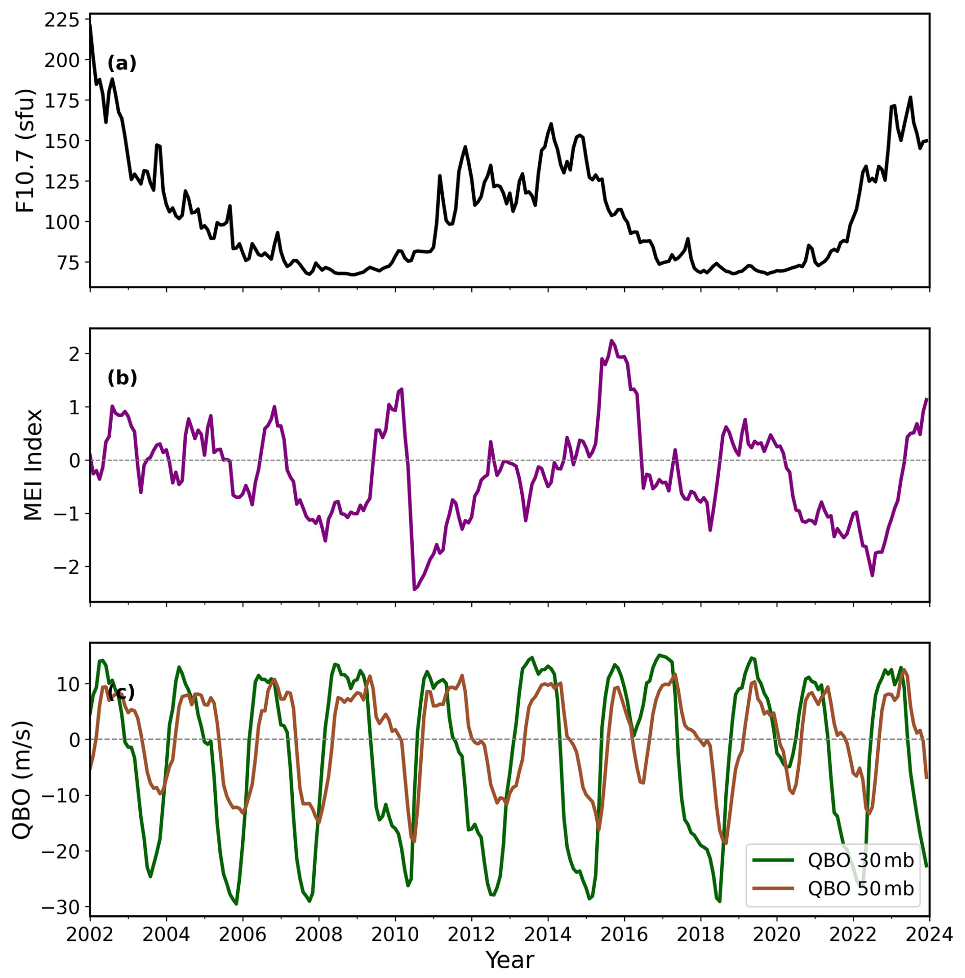
Figure 1 Time series of solar and geophysical indices from January 2002 to December 2023, used as explanatory variables. (a) The monthly mean solar radio flux at 10.7 cm (F_10.7) in solar flux units (sfu), which serves as a proxy for solar activity, clearly showing solar cycles 23 and 24. (b) The bimonthly Multivariate El Niño-Southern Oscillation (ENSO) Index (MEI), where positive values correspond to El Niño phases and negative values to La Niña phases. (c) The monthly mean zonal winds representing the Quasi-Biennial Oscillation (QBO) at two pressure levels in the tropics: 30 mb (dark green line) and 50 mb (sienna line). Negative (positive) values indicate easterly (westerly) wind regimes.

3 Results

3.1 Latitudinal and Temporal Evolution OH and E_p

Figure 2 reveals the temporal evolution of mesospheric OH airglow and gravity wave activity over the 22-year SABER observation. The top panel shows the OH_VER, which exhibits latitudinal and seasonal patterns consistent with the underlying photochemical processes governing OH production and loss in the mesosphere. The OH_VER displays seasonal variations with maximum values occurring during local December–January–February (DJF) and June–July–August (JJA) months at mid-latitudes, reaching peak emission rates of approximately 8–10 $\times {\mathrm{10}}^{-\mathrm{7}}$ W m⁻³ in both hemispheres. This seasonal pattern likely reflects the coupling between atomic hydrogen and ozone concentrations, both of which are modulated by seasonal changes in atmospheric dynamics and photochemistry (Xu et al., 2012; Gao et al., 2010). The latitudinal structure of OH_VER shows an asymmetry between hemispheres, with higher emission rates observed in the Northern Hemisphere (NH), particularly during DJF months. This hemispheric asymmetry can be attributed to differences in planetary wave activity and stratosphere-mesosphere coupling, which affect the transport of atomic oxygen and hydrogen species that control OH chemistry (Smith et al., 2013; Gao et al., 2011). The equatorial region exhibits relatively stable OH emission rates throughout the year, with values typically ranging between 4–6 $\times {\mathrm{10}}^{-\mathrm{7}}$ W m⁻³, consistent with the reduced seasonal variability expected in tropical latitudes where solar zenith angle variations are minimal.

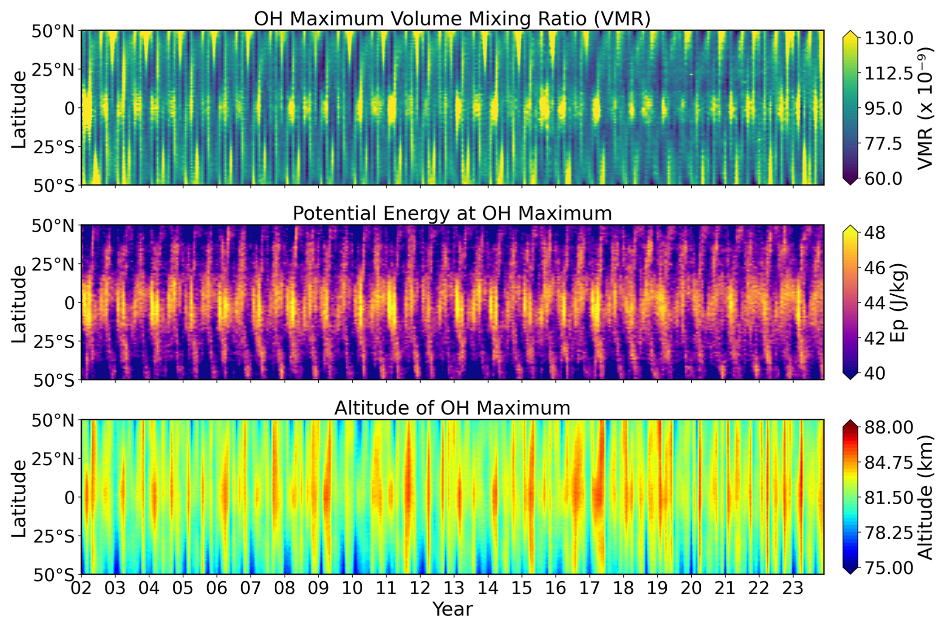
Figure 2 Temporal evolution (2002–2023) of zonally averaged parameters as a function of latitude. (Top) OH Maximum Volume Emission Rate (VER). (Middle) E_p at OH Maximum (E_p). (Bottom) Altitude of OH_VER Maximum.

The middle panel displays the E_p at the OH maximum altitude, providing characterization of gravity wave activity in the mesosphere. The E_p exhibits temporal and spatial variability, with values ranging from less than 36 J kg⁻¹ to over 48 J kg⁻¹. Features include increased gravity wave activity during local winter months at mid-latitudes, consistent with tropospheric wave generation and propagation conditions during these periods (Ern et al., 2011; Zhang et al., 2012). This seasonal pattern is consistent with findings from Ayorinde et al. (2024), who demonstrated that gravity wave E_p over South America shows seasonal dependence, with maximum values during JJA months when tropospheric forcing is largest. The spatial distribution of gravity wave activity shows hemispheric asymmetries, with higher E_p values in the NH. We note that our E_p values, measured at the OH peak altitude (∼87 km), do not show the pronounced winter mid-latitude peaks near 50° N/S reported by Liu et al. (2017) and Geller et al. (2013) at lower altitudes (50–100 km on a fixed grid). This difference arises because: (i) our analysis evaluates E_p at a single altitude (the OH peak) rather than across the full 50–100 km range where the strong stratospheric jet effect on gravity wave filtering is most pronounced; (ii) our latitude coverage extends only to ±50°, whereas the strongest winter GW activity occurs poleward of 50° where the polar night jet is strongest; and (iii) gravity wave E_p per unit mass at the OH peak altitude is modulated by local mesospheric conditions (temperature, stability) that differ from the stratospheric environment (Liu et al., 2017).

The equatorial region shows higher E_p values but with inter-annual variability, likely associated with the QBO and other tropical atmospheric phenomena (Ern et al., 2018). The solar cycle modulation is visible in both OH_VER and E_p throughout the observation period. The solar maximum around 2014–2015 corresponds to increased OH concentrations globally, reflecting the increased production of atomic hydrogen through solar Lyman-α radiation (Martin G. Mlynczak, 2013). E_p exhibits latitude-dependent solar cycle variations, indicating that solar forcing modulates gravity waves through multiple pathways: altered atmospheric stability and background winds (Liu et al., 2017). The bottom panel shows the altitude of the OH maximum, which varies between approximately 75 and 90 km with latitudinal and temporal patterns. The OH peak altitude exhibits a seasonal cycle, with higher altitudes during local DJF months in the NH and JJA months in the Southern Hemisphere (SH), consistent with seasonal changes in atmospheric temperature structure and the vertical distribution of atomic oxygen (Marsh et al., 2006).

3.2 Seasonal Cycles of OH and E_p

Figure 3 shows the seasonal decomposition analysis, providing characterization of the annual variations and the residual inter-annual variability. The seasonal cycles reveal the annual rhythms that characterize mesospheric variability. For OH_VER, the mid-latitude stations (50° N and 50° S) show DJF and JJA maxima, reaching peak values of 4–5 $\times {\mathrm{10}}^{-\mathrm{7}}$ µm at mid-latitudes. The tropical station (10° N) exhibits smaller seasonal variations. The E_p seasonal cycles show larger amplitudes, particularly at mid-latitudes, where DJF and JJA values can exceed their opposite seasons by factors of 2–3, with maxima reaching 7–15 J kg⁻¹. This reflects the seasonal dependence of gravity wave generation in the troposphere, with increased wave activity during these months when storm tracks are most active. The NH shows higher E_p values compared to the SH, particularly during DJF months, reflecting orographic and convective wave sources. Additionally, differences in the gravity wave environment between the two hemispheres, including the distribution of topographic features, jet stream characteristics, and convective activity. This may contribute to the observed hemispheric asymmetry in E_p (Ern et al., 2018; Geller et al., 2013). The residual time series (Fig. 3b) reveals inter-annual variability that remains after removing the seasonal patterns, showing evidence for solar cycle modulation, ENSO influences, and long-term trends. The OH_VER residuals show variations with evidence of solar cycle modulation, while the E_p residuals exhibit higher frequency variability with larger amplitude fluctuations.

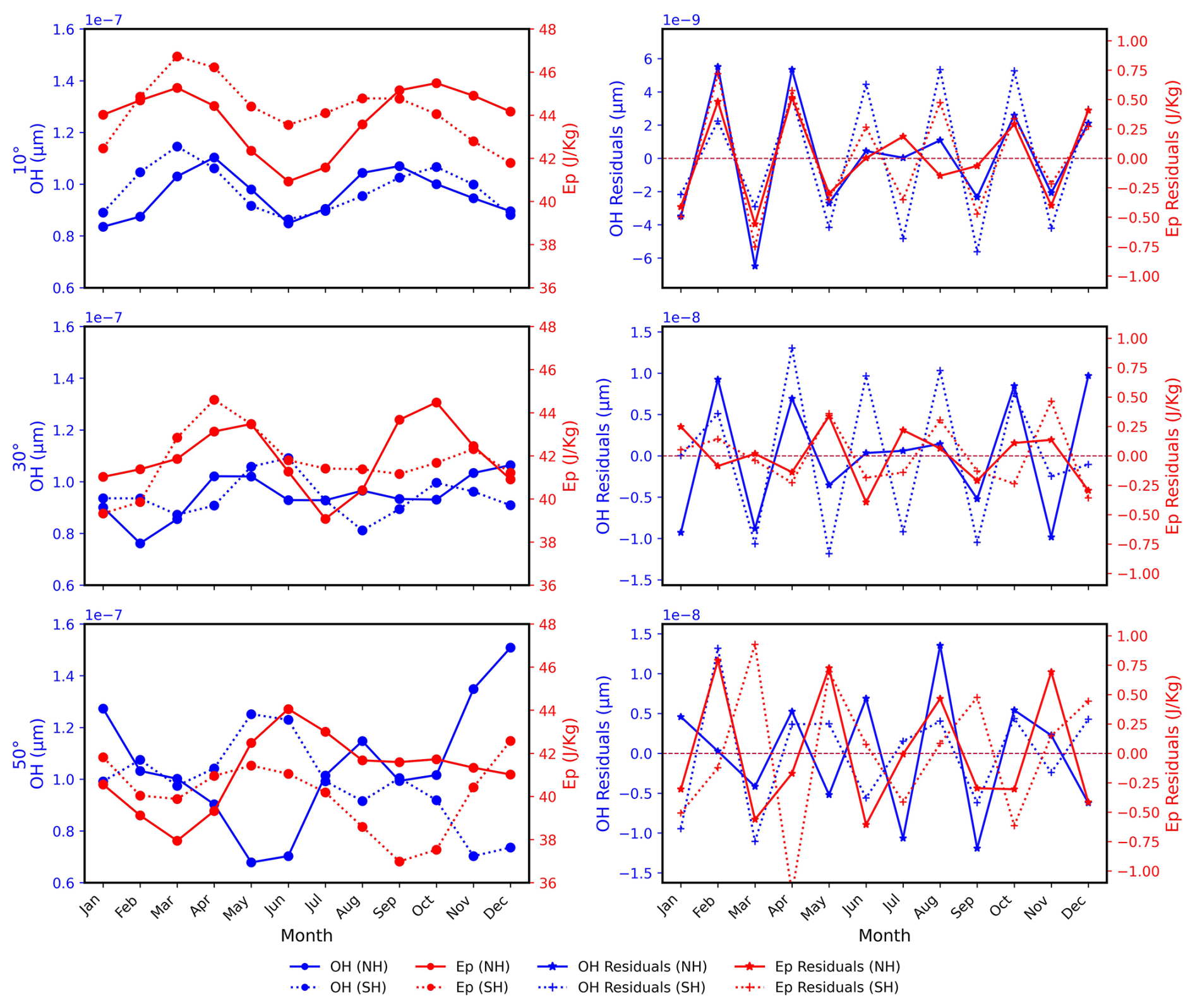
Figure 3 Mean seasonal cycles and residuals at different latitudes. (a) Mean seasonal cycle of OH_VER (left y-axis) and E_p (right y-axis) at 10, 30, and 60° latitude. The top panel corresponds to 10° latitude, the middle panel to 30° latitude, and the bottom panel to 60° latitude. Solid lines represent the Northern Hemisphere (NH) and dotted lines represent the Southern Hemisphere (SH). Blue lines correspond to OH, while red lines correspond to E_p. The figure shows distinct seasonal patterns with December–January–February (DJF) and June–July–August (JJA) representing the primary seasonal contrasts in each hemisphere. (b) Corresponding residuals from the mean seasonal cycle for each time series, revealing inter-annual variability and long-term trends after removing the dominant seasonal activities.

OH_VER seasonal cycles show strong latitudinal and hemispheric variations. At 50° latitude, both hemispheres exhibit maxima during local winter (DJF in NH, JJA in SH) with amplitudes of 0.4–0.5 $\times {\mathrm{10}}^{-\mathrm{7}}$ µm, driven by solar zenith angle and atmospheric dynamics. The seasonal amplitude decreases equatorward: ∼ 0.2–0.3 $\times {\mathrm{10}}^{-\mathrm{7}}$ µm at 30° (NH winter maximum) and minimal variation at 10° with near-symmetric hemispheric behavior. The E_p seasonal cycles display larger relative amplitudes, with mid-latitude (50°) maxima of 7–15 J kg⁻¹ which is 3–4 times the seasonal minima. Residual variability reveals inter-annual fluctuations including enhanced OH_VER during the 2014–2015 solar maximum and persistent hemispheric asymmetries throughout the observation period.

3.3 Latitudinal Profiles of Trends and Solar Responses

The linear trend analysis (Fig. 4) shows latitudinal patterns in the long-term evolution of both OH_VER and E_p over the 22-year observation period. We note that a 22-year time span, while among the longest continuous satellite records available for mesospheric studies, covers only approximately two solar cycles and is generally considered short for robust trend analysis. Moreover, the solar cycles covered here (cycles 23 and 24) had markedly different magnitudes, with cycle 24 being considerably weaker than cycle 23, which may affect the separation of solar-driven variability from long-term trends in the MLR analysis (Laštovička et al., 2006). These limitations should be kept in mind when interpreting the trend and solar response results presented below. Statistical significance of the trends is indicated by blue stars (p<0.05) and red stars (p≥0.05) overlaying the profiles, as detailed in the figure caption. For OH_VER (Fig. 4a–b), the annual trends are not statistically significant at the 95 % confidence level at most mid-latitude bins (25–50°), where the 95 % confidence intervals overlap zero despite negative central values. Near the equator (±15°), trends are weak and also not statistically significant. The magnitude of the OH trend central values ranges from −0.2 to +0.4 $\times {\mathrm{10}}^{-\mathrm{9}}$ µm per year. Seasonal decomposition reveals distinct DJF and JJA trend patterns: JJA trends are predominantly positive across all latitudes, particularly in NH subtropics, while DJF trends show hemispheric asymmetry – positive in the SH, variable in the NH – though individual latitude bins should be evaluated against their respective confidence intervals.

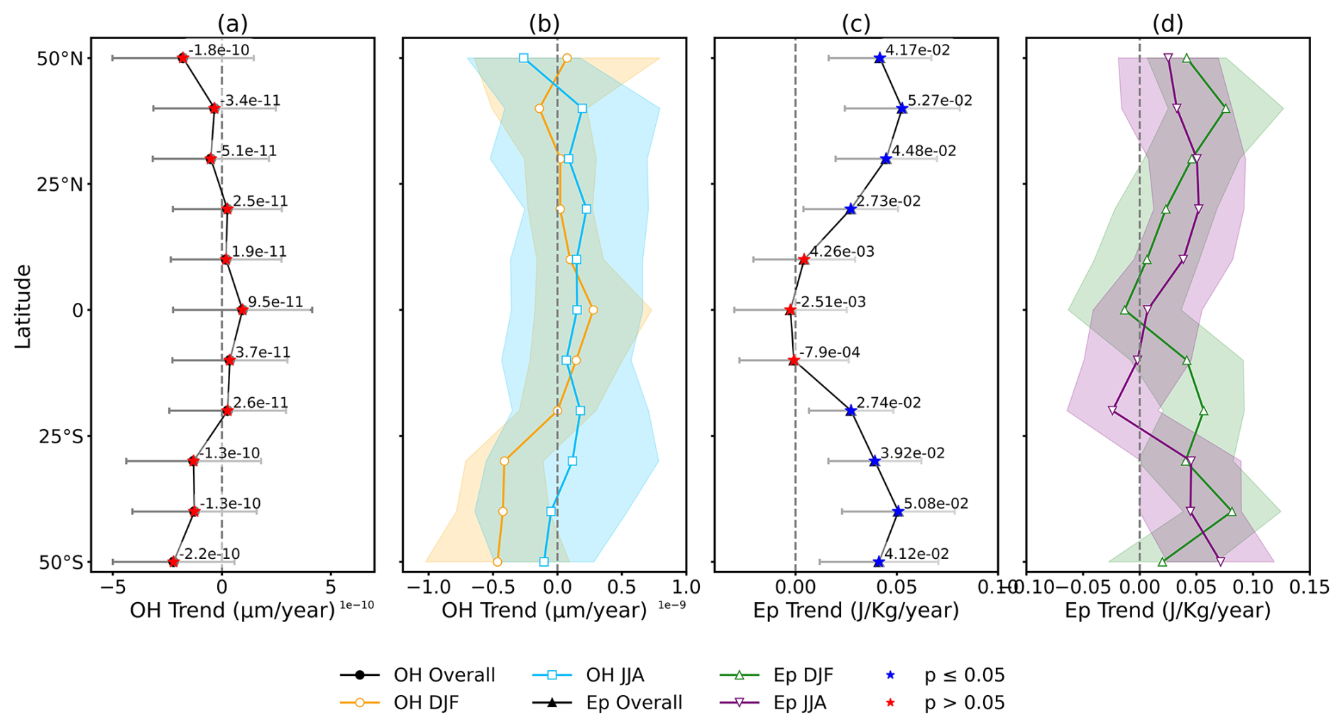
Figure 4 Latitudinal profiles of the linear trend. (a) Overall annual trend for OH_VER. (b) Seasonal trend for OH_VER during JJA (orange) and DJF (cyan). (c) Overall annual trend for E_p. (d) Seasonal trend for E_p during JJA (green) and DJF (purple). Error bars in (a, c) and shaded areas in (b, d) indicate the 95 % confidence interval of the trend coefficients. The blue stars overlaying the overall profile indicate statistically significant values (p<0.05), while red stars indicate values that are not statistically significant (p≥0.05).

E_p trends (Fig. 4c–d) differ from OH_VER, exhibiting stronger latitudinal gradients and larger relative amplitudes. Near the equator (±15°), the trends in potential energy (E_p) are weak and statistically insignificant, remaining close to zero. In contrast, statistically significant positive trends emerge in the mid-latitudes of both hemispheres (25 to 50°). We note that part of the observed E_p trend may reflect the upward shift of the OH emission layer (0.02–0.06 km yr⁻¹; see Fig. 10): because E_p per unit mass increases with altitude as atmospheric density decreases, a rising OH peak altitude produces an apparent increase in E_p even without a real change in gravity wave activity. This effect is discussed quantitatively in Sect. 4.

In the NH, the E_p trend strengthens from approximately 0.03 J kg⁻¹ yr⁻¹ at 25°N to a peak of about 0.05 J kg⁻¹ yr⁻¹ between 30° N and 40° N, before decreasing to around 0.04 J kg⁻¹ yr⁻¹ at 50° N. A similar pattern is observed in the SH, where the trend peaks at approximately 0.05 J kg⁻¹ yr⁻¹ around 40° S. A seasonal analysis reveals distinct patterns. During June–July–August (JJA), trends are consistently positive across all latitudes. However, during December–January–February (DJF), the patterns show hemispheric asymmetry. The NH mid-latitudes exhibit strong positive trends, reaching up to 8–10 J kg⁻¹ yr⁻¹, whereas the SH trends are smaller and more variable.

The solar response analysis (Fig. 5) shows the relationship between solar variability and mesospheric processes across all latitudes. As with the trend analysis, statistical significance is indicated by blue and red stars overlaying the profiles (see figure caption for details). For OH_VER (Fig. 5a–b), the solar response is positive across all latitudes with an equatorial maximum reaching values of 0.8–1.0 $\times {\mathrm{10}}^{-\mathrm{7}}$ µm per 100 sfu (solar flux units). JJA responses are larger than DJF responses, particularly in the NH. The hemispheric asymmetries in solar response are present during DJF months, with the SH showing larger responses than the NH. The E_p solar response (Fig. 5c–d) shows patterns with both positive and negative responses depending on latitude and season. The annual response shows positive values in tropical regions and negative values at mid-latitudes. The seasonal decomposition of E_p solar response shows differences between JJA and DJF patterns. JJA responses are positive across most latitudes, while DJF responses show hemispheric asymmetries with positive responses in the SH and negative responses in the NH at mid-latitudes.

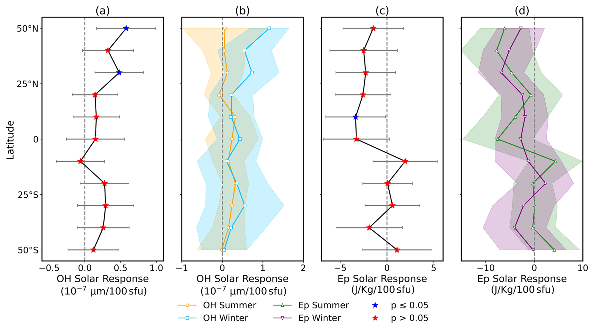
Figure 5 Latitudinal profiles of the solar response. (a) Overall annual response for OH_VER. (b) Seasonal response for OH_VER during JJA (orange) and DJF (cyan). (c) Overall annual response for E_p. (d) Seasonal response for E_p during JJA (green) and DJF (purple). Error bars in (a, c) and shaded areas in (b, d) indicate the 95 % confidence interval of the regression coefficients. The blue stars overlaying the overall profile indicate statistically significant values (p<0.05), while red stars indicate values that are not statistically significant (p≥0.05).

The hemispheric asymmetries in solar responses (Fig. 5) show contrasting behavior between OH and E_p. For OH (Fig. 5a–b), both hemispheres show positive solar responses, with the SH exhibiting larger responses at mid-latitudes during DJF months. The E_p solar responses (Fig. 5c–d) show hemispheric differences during the DJF months. The SH displays positive solar responses at most latitudes, while the NH shows negative solar responses at mid-latitudes during DJF.

3.4 Quasi-Biennial Oscillation and ENSO Responses

Figures 6 and 7 examine the responses of mesospheric OH and gravity wave activity to two primary modes of tropical atmospheric variability: the QBO and the ENSO. The QBO response analysis (Fig. 6) reveals patterns of mesospheric coupling to stratospheric wind oscillations. Statistical significance of the responses is indicated by blue stars (p<0.05) and red stars (p≥0.05) overlaying the overall profiles, as shown in the figure captions.

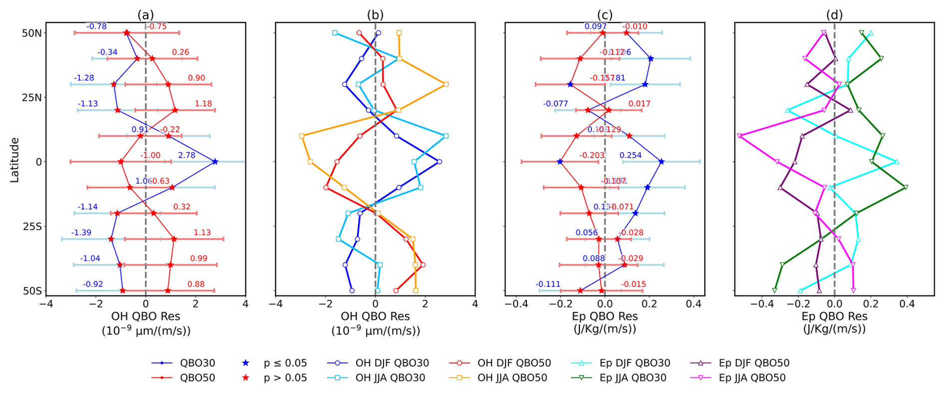
Figure 6 Latitudinal profiles of the QBO response for OH_VER and E_p. (a, c) The overall annual response to QBO at 30 and 50 mb for OH_VER and E_p, respectively. (b, d) The seasonal (JJA and DJF) response to QBO at 30 and 50 mb for OH_VER and E_p, respectively. Different colors and markers correspond to the specific proxy and season as detailed in the legend. Error bars indicate the 95 % confidence interval of the coefficients. The blue stars overlaying the overall profile indicate statistically significant values (p<0.05), while red stars indicate values that are not statistically significant (p≥0.05).

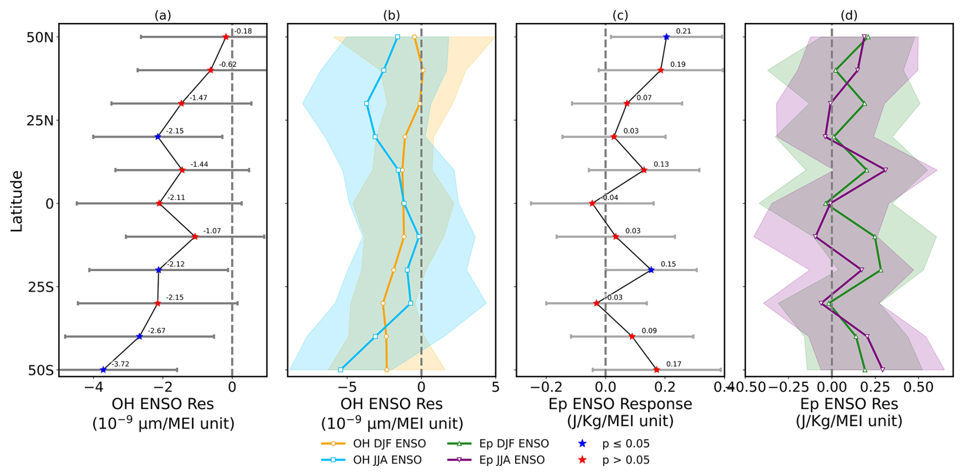
Figure 7 Latitudinal profiles of the ENSO response. (a) Overall annual response for OH_VER. (b) Seasonal response for OH_VER during JJA (orange) and DJF (cyan). (c) Overall annual response for E_p. (d) Seasonal response for E_p during JJA (green) and DJF (purple). Error bars in (a, c) and shaded areas in (b, d) indicate the 95 % confidence interval of the regression coefficients. The blue stars overlaying the overall profile indicate statistically significant values (p<0.05), while red stars indicate values that are not statistically significant (p≥0.05).

The OH response to the QBO in Fig. 6a shows opposite responses between the equator and midlatitudes. Around the equator (±15°), QBO30 produces positive responses ($+\mathrm{2.8}\times {\mathrm{10}}^{-\mathrm{9}}$ µm m s⁻¹), while QBO50 induces negative values near $-\mathrm{1.0}\times {\mathrm{10}}^{-\mathrm{9}}$ µm (m s⁻¹). In contrast, both hemispheres at 25–50° show weaker and opposite-signed trends: in the NH, QBO30 responses are negative (−0.3 to $-\mathrm{0.8}\times {\mathrm{10}}^{-\mathrm{9}}$ µm m s⁻¹) while QBO50 yields positive (+0.2 to $+\mathrm{0.9}\times {\mathrm{10}}^{-\mathrm{9}}$ µm m s⁻¹). The SH shows a similar pattern, with QBO30 negative (−0.9 to $-\mathrm{1.4}\times {\mathrm{10}}^{-\mathrm{9}}$ µm m s⁻¹) and QBO50 positive ($\sim +\mathrm{0.9}$ to $+\mathrm{1.1}\times {\mathrm{10}}^{-\mathrm{9}}$ µm m s⁻¹). Thus, equatorial OH is modulated with opposite phase between QBO30 and QBO50, while midlatitudes show a smaller but consistent opposing trend. Around the equator, variability is evident, with QBO30 responses shifting between positive and negative depending on season, particularly during JJA. In the NH midlatitudes, QBO50 trends dominate as positive anomalies, whereas in the SH midlatitudes, both QBO30 and QBO50 yield small but oppositely signed contributions, with seasonality introducing scatter. Overall, the seasonal structure indicates that the equatorial trend is the largest and most sensitive to phase, while midlatitudes remain weaker and seasonally modulated.

E_p responses (Fig. 6c) to the QBO also show equatorial–midlatitude contrasts. At the equator (±15°), E_p regressions are mixed, with QBO30 alternating between slightly negative (−0.11 to −0.08 J kg⁻¹ m s⁻¹) and positive (+0.06 to +0.09 J kg⁻¹ m s⁻¹), while QBO50 remains near zero to slightly negative (−0.07 to −0.20 J kg⁻¹ m s⁻¹). In the NH 25–50° N, E_p responses to QBO30 are positive, peaking around +0.25 J kg⁻¹ (m s⁻¹), while QBO50 trends slightly negative (−0.01 to −0.20 J kg⁻¹ m s⁻¹). In the SH midlatitudes, QBO30 is positive (+0.05 to +0.09 J kg⁻¹ m s⁻¹), with QBO50 negative (−0.1 to −0.2 J kg⁻¹ m s⁻¹). This indicates that E_p is modulated by the QBO in the NH midlatitudes, particularly by QBO30.

Figure 6d shows strong seasonal and latitudinal dependence in QBO modulation. Equatorial E_p remains near-zero or negative year-round, whereas NH mid-latitudes display seasonally dependent responses: positive under QBO30 during JJA, negative or weak under QBO50. In the SH midlatitudes, E_p responses are less consistent but show positive anomalies under QBO30, especially during JJA, and negative or near-zero under QBO50. Seasonality thus enhances the midlatitude asymmetry, with NH responses larger and more coherent than SH.

The ENSO response analysis (Fig. 7) shows ENSO responses of OH and E_p across latitude bands. As indicated by the blue and red stars in the figure, statistical significance varies with latitude (see figure caption for details). Figure 7a indicates that OH ENSO responses are negative across all latitudes, with the largest values in the SH ($-\mathrm{3.72}\times {\mathrm{10}}^{-\mathrm{7}}$ µm MEI at 50° S, $-\mathrm{2.67}\times {\mathrm{10}}^{-\mathrm{7}}$ µm MEI at 35° S) and smaller values in the NH ($-\mathrm{2.15}\times {\mathrm{10}}^{-\mathrm{7}}$ µm MEI at 25° N, weakening to $-\mathrm{0.18}\times {\mathrm{10}}^{-\mathrm{7}}$ µm MEI at 50° N). Around the equatorial region (±15°), OH decreases are present ($-\mathrm{2.11}\times {\mathrm{10}}^{-\mathrm{7}}$ µm MEI at the equator, $-\mathrm{2.12}\times {\mathrm{10}}^{-\mathrm{7}}$ µm MEI at 15° S). Figure 7b separates seasonal signals, showing that both DJF (orange) and JJA (blue) responses are negative throughout, with larger negative anomalies during JJA, especially in the tropics and subtropics, while DJF shows weaker responses. Figure 7c depicts E_p ENSO response, which is positive across latitudes. Near the equator (±15°), the response is small (0.03–0.04 J kg⁻¹ MEI), increasing toward higher latitudes: 0.21 J kg⁻¹ MEI at 50° N and 0.17 J kg⁻¹ MEI at 50° S. Figure 7d shows the seasonal breakdown of E_p responses: both DJF (green) and JJA (purple) display positive anomalies across most latitudes, with larger responses in JJA, particularly in the equatorial and SH regions, whereas DJF is more moderate.

3.5 Correlation Analysis and Index Relationships

Figure 8 provides the analysis of the correlation patterns between deseasonalized and detrended OH_VER and E_p time series and various atmospheric indices. The correlation analysis for OH_VER (Fig. 8c) shows positive correlations across all latitudes with maximum values of 0.6–0.7 (95 % confidence interval [CI]: 0.5–0.8, estimated via Fisher's z-transformation) in tropical regions. The ENSO correlations show a latitudinal structure with maximum values in tropical and subtropical regions, reaching correlations of 0.3–0.4 (95 % CI: 0.1–0.5). The QBO correlations are weaker, with the 30 mb index exhibiting larger correlations than the 50 mb index in most regions. The E_p correlations (Fig. 8d) show different patterns compared to OH_VER. The solar correlations are weaker and more variable, with both positive and negative values depending on latitude. The ENSO and QBO correlations for E_p show latitudinal variations with larger correlations in tropical and subtropical regions. The QBO correlations show differences between the 30 and 50 mb indices. The ENSO correlations show hemispheric asymmetries, with larger correlations in the NH.

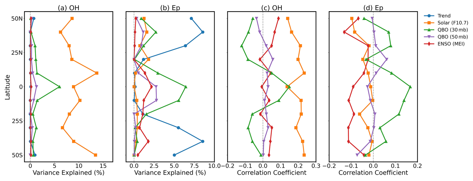
Figure 8 Latitudinal structure of the relationships between hydroxyl (OH), E_p (E_p), and climate modes. (a, b) Percentage of variance in deseasonalized monthly mean OH peak concentration and E_p per unit mass (E_p) at the altitude of the OH peak, respectively, explained by individual predictors. The values are derived from a multiple linear regression (MLR) model applied at each 10° latitude. (c, d) Pearson correlation coefficients between the monthly mean time series of OH peak concentration and E_p, respectively, and the climate modes. The predictors, indicated in the legend, are a linear trend (Trend), the F_10.7 cm solar radio flux (Solar), the standardized Quasi-Biennial Oscillation (QBO) at 30 and 50 mb, and the Multivariate ENSO Index (ENSO-MEI).

The variance decomposition analysis (Fig. 8) shows the percentage of variance explained by each predictor as a function of latitude. In the equatorial region (±15°), OH variance (Fig. 8a) is influenced by solar forcing (≈ 6–8 %) with small contributions from QBO and ENSO, while E_p variance (Fig. 8b) shows contributions from QBO (up to ∼5 %) and modest ENSO impact. Correlations (Fig. 8c–d) in the equator show: OH correlates positive with solar but near-zero with QBO and ENSO, whereas E_p shows positive correlation with QBO (30 and 50 mb) and weaker links to solar and ENSO. In the NH (25–50° N), OH variance is dominated by solar (∼10–15 %) with little ENSO or QBO contribution, while E_p variance is split across solar, QBO, and the long-term trend, each explaining a few percent. OH is positively correlated with solar forcing, while E_p shows positive correlations with QBO and trend. In the SH (25–50° S), OH variance is solar-driven (10–15 %), with ENSO explaining a small fraction, whereas E_p variance shows trend and QBO contributions (up to 5–7 %). OH links mainly to solar, while E_p shows positive associations with QBO and trend.

3.6 Altitude-Latitude Climatology and Trends

Figure 9 presents the altitude-latitude structure of the OH and E_p climatology along with the spatial distribution of linear trends. In Fig. 9a (OH_VER), the emission layer is largest near the mesopause around 85–90 km, forming a maximum at the equator (±15°) with relatively uniform latitudinal distribution but a weakening in the NH midlatitudes (25–50° N). In the SH midlatitudes (25–50° S), OH emissions appear somewhat more extended vertically but weaker compared to the equatorial peak. In Fig. 9b (E_p, the gravity wave potential energy per unit mass), the climatology shows a broad maximum above 85 km, largest near the equator, extending well into the upper mesosphere and lower thermosphere. The equatorial region (±15°) shows the largest and vertically thickest values of E_p, while both hemispheres (25–50° N and 25–50° S) show weaker enhancements that do not extend as high as at the equator. The SH shows slightly larger midlatitude E_p values than the NH. In Fig. 9c (linear trend slope of OH_VER), the equatorial region (±15°) is dominated by positive trends between 80–95 km, indicating an intensification of OH emissions. In contrast, both hemispheres (25–50° N and 25–50° S) display weaker and less consistent signals: trends are largely not statistically significant, with some patches of negative slopes below 80 km and near 90 km. The SH exhibits more coherent negative trends below 80 km, whereas the NH shows smaller-scale variability without statistical significance.

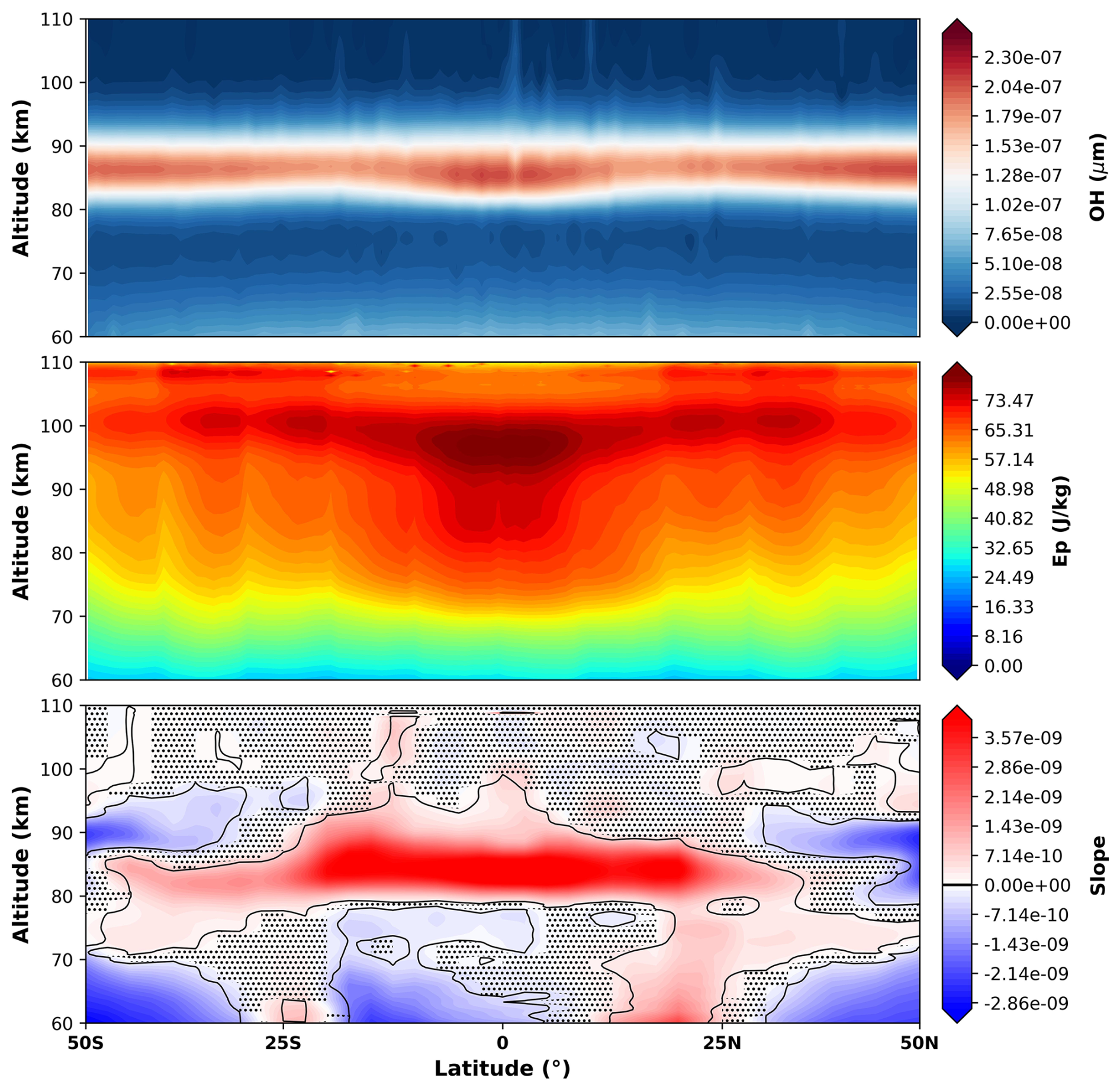
Figure 9 Climatology and linear trend. The top and middle panels show the climatological mean of OH_VER (in µm) and E_p (in J kg⁻¹), respectively, as a function of latitude and altitude. The bottom panel shows the slope of the linear trend of OH_VER. Stippling in the bottom panel indicates regions where the trend is statistically significant at the 95 % confidence level.

The altitude trends and solar responses of the OH peak (Fig. 10) show the vertical structure changes of the mesospheric OH layer over the observation period. Statistical significance is indicated by blue stars (p<0.05) and red stars (p≥0.05) overlaying the overall profiles, as detailed in the figure caption. In Fig. 10a, the linear trend in the OH emission peak altitude is positive across all latitudes, with values around 0.02–0.04 km yr⁻¹ near the equatorial region (±15°). In the NH midlatitudes (25–50° N), the overall trend increases slightly, peaking near 0.05 km yr⁻¹ during JJA, while DJF trends remain at ∼0.02 km yr⁻¹. In the SH midlatitudes (25–50° S), the trends are also positive but more seasonally contrasted: JJA trends are larger (up to ∼0.05–0.06 km yr⁻¹), whereas DJF trends are closer to ∼0.01–0.02 km yr⁻¹. In Fig. 10b, the solar response (km 100 sfu) shows a latitude-dependent asymmetry. Near the equator (±15°), the overall response is small, close to zero, but seasonally distinct – negative during JJA and positive to near zero during DJF. In the NH midlatitudes (25–50° N), the overall solar response remains small but slightly positive, while JJA responses are near zero and DJF responses show negative values. By contrast, in the SH midlatitudes (25–50° S), the overall solar response is negative, dominated by negative values during JJA, while DJF responses are closer to zero or negative.

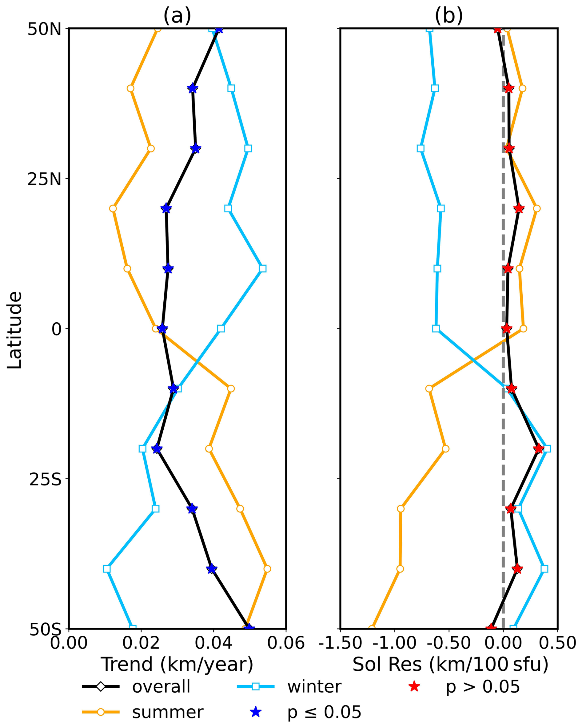
Figure 10 Latitudinal variation of (a) the linear trend in km yr⁻¹ and (b) the solar response (Sol Res) in km 100 sfu. The results are shown for the overall period (black line with diamonds), for JJA months (orange line with circles), and for DJF months (cyan line with squares). The vertical dashed line in panel (b) indicates zero response. The blue stars overlaying the overall profile indicate statistically significant values (p<0.05), while red stars indicate values that are not statistically significant (p≥0.05).

3.7 Semiannual Oscillations and their Annual Cycles

The seasonal analysis employs harmonic decomposition techniques to extract annual oscillation (AO) and SAO components from the deseasonalized time series, following the methodology established by Gu et al. (2024) for OH airglow emission analysis. Sinusoidal functions are fitted to monthly climatological data to quantify amplitude and phase characteristics. We decompose seasonal cycles into AO and SAO components via least-squares harmonic fitting, where AO captures solar-driven annual variations and SAO represents semiannual oscillations linked to equinoctial dynamics and stratospheric circulation. The amplitude represents the magnitude of seasonal variation relative to the annual mean, while the phase indicates the timing of maximum values throughout the year, providing insights into the physical mechanisms controlling seasonal variability in mesospheric OH chemistry and gravity wave activity.

The seasonal climatology (Fig. 11) reveals the annual and semi-annual patterns that drive mesospheric variability. In Fig. 11a, OH_VER shows a semiannual cycle with equatorial maxima (±15°) around April–May and October–November, while minima occur during solstitial months. In the NH midlatitudes (25–50° N), OH values are weaker overall, with enhancements in late spring and autumn. In the SH midlatitudes (25–50° S), OH intensities are lower, though peaks are seen in May–June and November–December. In Fig. 11b, E_p exhibits largest values at the equator, with broad enhancements during March–April and again in September–October, consistent with semiannual variability. In the NH (25–50° N), E_p remains relatively weak year-round, with a faint enhancement in Boreal autumn. The SH (25–50° S) shows similarly weak E_p values, with no distinct seasonal maxima compared to the equatorial dominance. In Fig. 11c, the OH peak altitude displays a semiannual oscillation at the equator, reaching higher altitudes (∼83–85 km) in April–May and October–November, and lower altitudes (∼78–80 km) during solstitial months. In the NH (25–50° N), the peak altitude is elevated mainly in April–May, while in the SH (25–50° S), the main enhancement occurs during October–November. Overall, the equatorial region controls the dominant semiannual cycle, while the midlatitudes show weaker, seasonally shifted responses.

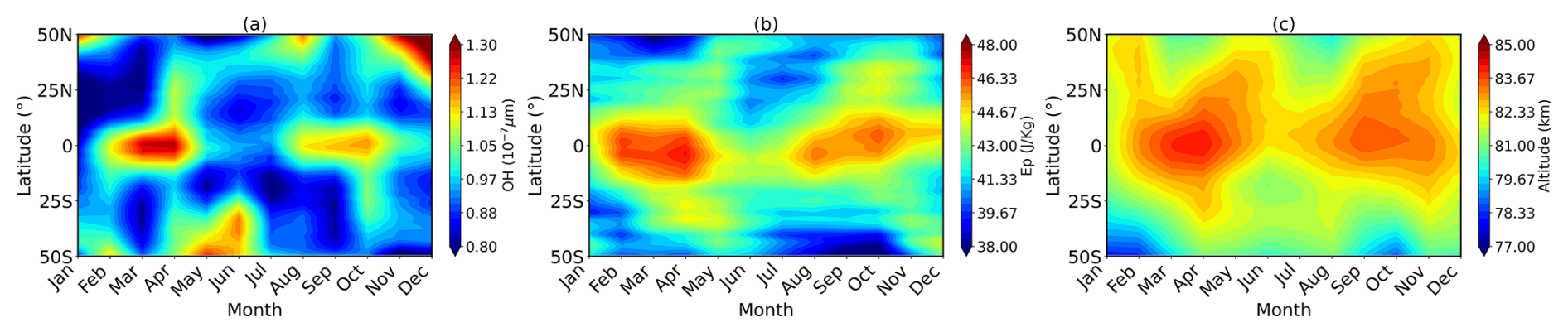
Figure 11 Mean seasonal climatology as a function of latitude and month for (a) OH_VER (in 10⁻⁷ µm), (b) E_p, E_p (in J kg⁻¹), and (c) the altitude of the OH peak (in km).

Figure 12 shows the harmonic analysis which estimates the amplitude and phase characteristics of AO and SAO components. In the semiannual oscillation (SAO) panels (left column), OH relative amplitude (panel a) peaks at the equator (±15°) around 10–12 %, while in the SH midlatitudes (25–50° S) the amplitude reaches comparable values near 25° S but decreases further poleward. In the NH (25–50° N), amplitudes are weaker, staying below 8 %. The SAO phase indicates maxima occurring earlier in the year at higher latitudes and shifting toward later days near the equator. E_p relative amplitude (Fig. 12c) also peaks in the SH (25–50° S) with values near 4–5 %, while equatorial amplitudes are weaker (∼2–3 %), and NH values remain low (<2 %). The SAO altitude amplitude (Fig. 12e) is largest at the equator, approaching ∼1 km, and decreases steadily toward both hemispheres, with values around 0.6 km in the midlatitudes; phases are nearly flat across latitudes.

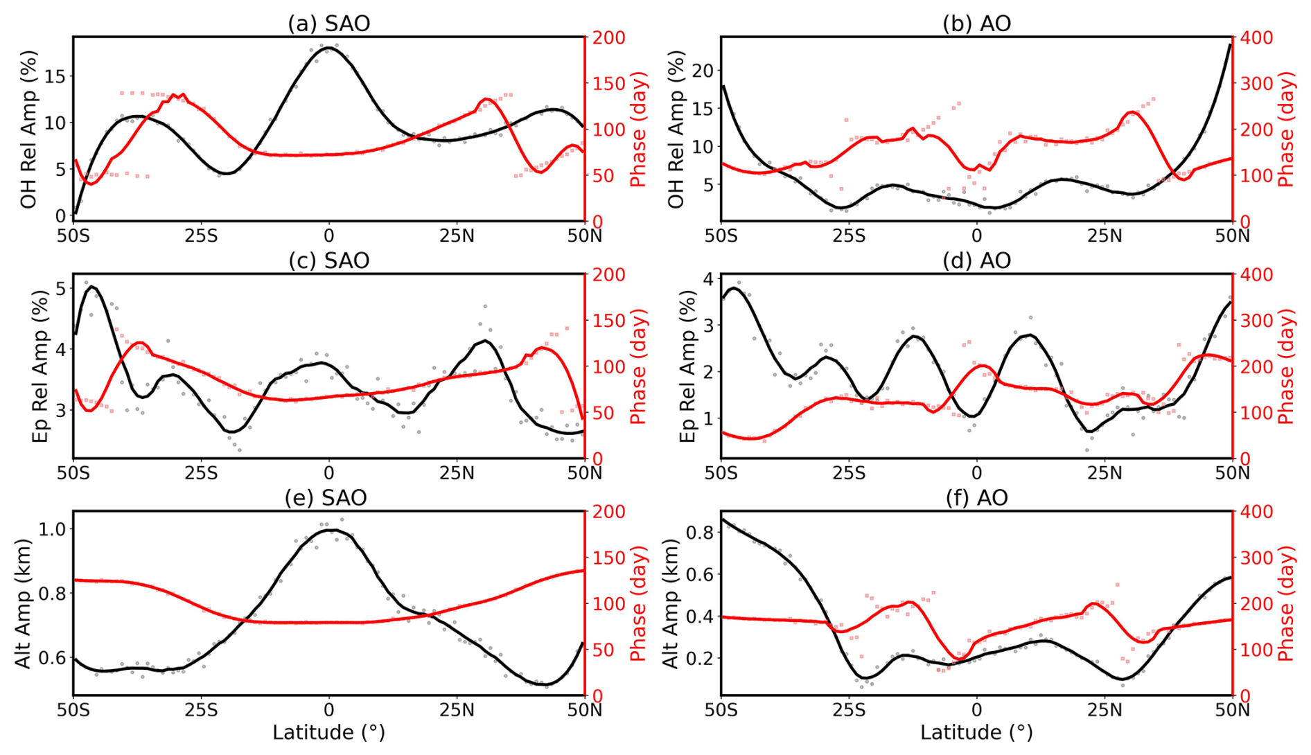
Figure 12 Latitudinal variations of the amplitude (black lines, left axes) and phase (red lines, right axes) for the (left column) SAO and (right column) AO. The rows correspond to different parameters: (a, b) OH relative amplitude (%), (c, d) E_p relative amplitude (%), and (e, f) altitude amplitude (km). Phase represents the day of maximum and is given in days. The faint points (gray circles for amplitude, red squares for phase) represent the binned data, while the solid lines are smoothed fits.

In the annual oscillation (AO) panels (right column), OH relative amplitude (Fig. 12b) shows larger signals in the SH (25–50° S), peaking above 15–20 %, while equatorial values are lower (∼5–7 %), and the NH midlatitudes (25–50° N) show amplitudes around 10 %. Phases indicate hemispheric asymmetry, with maxima occurring later in the year in the NH compared to the SH. E_p relative amplitude (Fig. 12d) exhibits alternating peaks across latitude, with larger amplitudes in the SH (∼3–4 %), weaker equatorial values (<2 %), and NH amplitudes (∼2 %). Finally, altitude amplitude (Fig. 12f) shows equatorial suppression (∼0.2–0.3 km) compared to enhancements in the midlatitudes: ∼0.6 km in the SH (25–50° S) and ∼0.4–0.5 km in the NH (25–50° N). AO phases are more variable, reflecting hemispheric differences and less coherent timing compared to the SAO.

3.8 Thermal and Non-Thermal Contributions of OH Trend

The decomposition analysis separates temperature-driven effects from residual non-thermal processes in OH variability. The methodology integrates SABER satellite observations with geophysical indices representing atmospheric drivers (F_10.7, K_p, MEI, QBO) using a two-stage MLR framework. After aggregating data into 10° latitude bins and removing seasonal periodicities, the deseasonalized anomalies are modeled using:

$$\begin{array}{}\text{(9)}& Y\left(t\right)=C_{\mathrm{0}}+C_{\mathrm{1}}\cdot t+\sum _{i=\mathrm{2}}^N{C}_i\cdot P_i\left(t\right)+\mathit{ϵ}\left(t\right)\end{array}$$

where Y(t) represents OH or temperature, C₁ is the linear trend coefficient, P_i(t) are the geophysical proxies, and ϵ(t) is residual variability. The decomposition leverages the temperature dependence of OH chemistry. The temperature-driven component of OH trends is calculated as:

$$\begin{array}{}\text{(10)}& {\text{Trend}}_{\text{OH,Temp}}=\stackrel{\mathrm{‾}}{\text{OH}}\cdot \mathit{\beta }\cdot {\text{Trend}}_{\text{Temp}}\end{array}$$

where β is the temperature sensitivity coefficient, the residual trend is then isolated as:

$$\begin{array}{}\text{(11)}& {\text{Trend}}_{\text{OH,Res}}={\text{Trend}}_{\text{OH,Obs}}-{\text{Trend}}_{\text{OH,Temp}}\end{array}$$

This decomposition is applied to both trends and responses to each proxy, providing quantitative separation of thermal versus non-thermal mechanisms. Figure 13 presents the decomposition of OH trends and the correlation between OH and temperature trends. In Fig. 13a, the observed OH trend is negative across all latitudes. At the equator (±15°), OH trends are close to zero, showing weak decreases. In the NH (25–50° N), the trend is negative, ranging between −1 and $-\mathrm{3}\times {\mathrm{10}}^{-\mathrm{10}}$ µm yr⁻¹, while in the SH (25–50° S) the decline reaches values near −4 to $-\mathrm{5}\times {\mathrm{10}}^{-\mathrm{10}}$ µm yr⁻¹. Figure 13b shows that temperature trends at the OH peak altitude are negative across latitudes, with the cooling ($\sim -\mathrm{0.15}$ K yr⁻¹) near the equator, weakening toward the midlatitudes in both hemispheres, where values range around −0.07 to −0.1 K yr⁻¹. Figure 13c shows the decomposition of the OH trend: the temperature-driven component (green) accounts for most of the negative signal, especially at the equator (±15°) and in the SH (25–50° S). A positive residual component (purple) emerges across latitudes, partly offsetting the cooling effect. This residual is larger in the midlatitudes of both hemispheres, suggesting additional drivers beyond temperature sustain OH emission levels despite the cooling background.

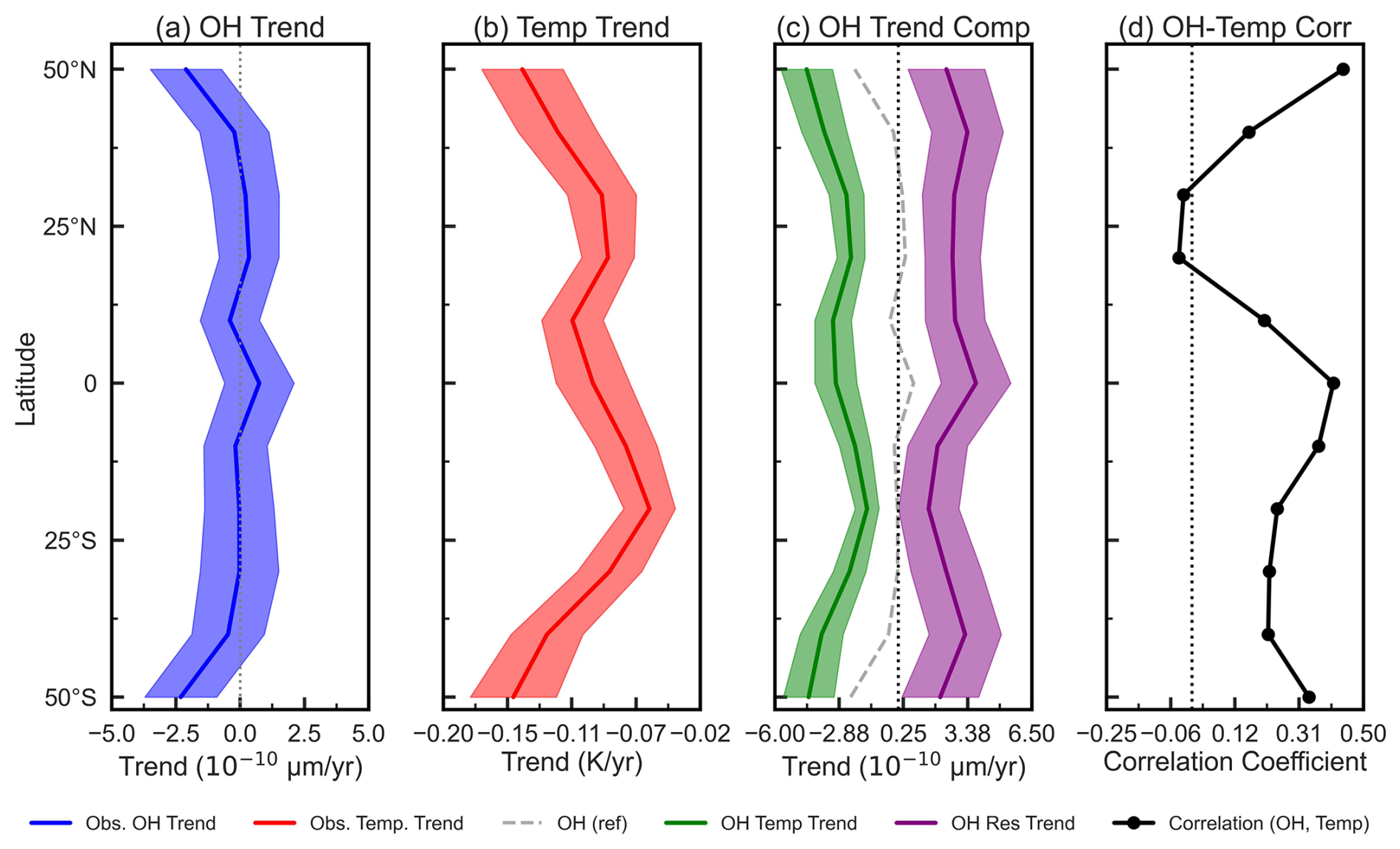
Figure 13 Decomposition of the linear trend in OH_VER and its correlation with temperature. (a) The observed latitudinal profile of the OH trend. (b) The observed latitudinal profile of the temperature trend at the OH peak altitude. (c) The observed OH trend (dashed gray) is decomposed into a component driven by the temperature trend (green) and a residual trend (purple). (d) The correlation coefficient between the OH and temperature trends. Shaded areas indicate the uncertainty.

The correlation coefficient between the OH and temperature trends (Fig. 13d) ranges from −0.25 to 0.5. Peak values of 0.4–0.5 occur in several latitude bands, consistent with the temperature dependence of the H + O₃ reaction rate. The correlation reaches a minimum of −0.25 near 25° N, indicating an anti-correlation in the Northern Hemisphere subtropics. This sign reversal points to non-thermal processes, such as changes in the Brewer–Dobson circulation or hemispheric asymmetries in wave-driven transport, that oppose the thermochemical response. Away from this minimum, the correlation returns to positive values but remains below 0.5 at all latitudes, indicating that non-thermal contributions persist across the globe. The correlation analysis in Fig. 13d thus complements the decomposition in Fig. 13c, confirming that thermal effects account for only part of the OH trend and that non-thermal processes dominate in the Northern Hemisphere subtropics.

4 Discussion

The observed correlation coefficients of 0.3–0.7 (95 % CI: 0.1–0.8) between OH VER and gravity wave E_p (Fig. 8) are consistent with the coupling mechanisms predicted by the dynamical-chemical models of Walterscheid et al. (1987) and Schubert et al. (1991). The physical basis involves two pathways: (i) gravity wave-induced temperature perturbations modulate the rate constant of the H + O₃ → OH^* + O₂ reaction (Minschwaner et al., 2011; Tarasick and Shepherd, 1992), and (ii) vertical advection by gravity waves displaces reactive species (O₃, H, O) across the steep vertical gradients near the OH layer, altering instantaneous production rates (Walterscheid et al., 1987; Li et al., 2011). We acknowledge, however, that a contribution from co-varying background conditions cannot be entirely excluded: both OH emission intensity and E_p per unit mass depend on local temperature and atmospheric stability, so that changes in the mean thermal state could drive correlated variations in both quantities without a direct causal link. Nevertheless, two features of the observed correlations argue against a purely spurious relationship. First, the correlation exhibits systematic latitude and season dependence, peaking during winter at mid-latitudes (reaching 0.7) and weakening to ∼0.3 at the equator. A temperature-driven spurious correlation would not produce this specific pattern, which instead matches the expected behaviour of gravity wave–OH coupling: during winter, mid-latitude gravity waves have longer vertical wavelengths that maintain phase coherence across the ∼8 km thick OH emission layer, producing stronger wave-induced emission fluctuations (Taylor et al., 2009; Ejiri et al., 2003; Nielsen et al., 2012). Second, the decomposition analysis (Fig. 13) demonstrates that temperature-driven effects account for only part of the OH variability, with substantial non-thermal residuals – a result inconsistent with temperature being the sole common driver. The weaker equatorial correlations (∼0.3) may reflect the broader gravity wave spectrum present in the tropics, where diverse source mechanisms (convection, shear instability) generate waves spanning a wide range of vertical wavelengths (Sato et al., 2009; Alexander et al., 2010). Waves with vertical wavelengths shorter than the OH layer thickness undergo phase cancellation that attenuates the integrated emission response (Vargas et al., 2007), reducing the net observed correlation.

The solar response (Fig. 5) shows OH responds positively across all latitudes with an equatorial maximum of 0.8–1.0 $\times {\mathrm{10}}^{-\mathrm{7}}$ W m⁻³ per 100 sfu, arising from Lyman-α photo-dissociation of H₂O producing atomic hydrogen for OH production (Martin G. Mlynczak, 2013). Solar forcing explains 10 %–15 % of OH variance at mid-latitudes (Fig. 8) (Gao et al., 2010; Fytterer et al., 2015). Gravity wave E_p shows weaker solar responses with hemispheric asymmetries. The mechanism by which solar variability influences gravity wave propagation is indirect: enhanced solar UV heating modifies the stratospheric temperature gradient and thereby the zonal mean wind, which controls the critical-level filtering of upward-propagating gravity waves (Gray et al., 2010; Liu et al., 2017). We note that while Gray et al. (2010) documented the solar influence on stratospheric temperatures and winds through the UV–ozone feedback pathway, the evidence for a direct solar modulation of polar vortex strength remains uncertain, and tropospheric forcing of the vortex is likely dominant. The hemispheric asymmetry in E_p solar response is consistent with the mechanism described by Lieberman et al. (2013), whereby background zonal winds filter gravity waves, and the filtering efficiency depends on the wind strength, which itself responds to solar-induced changes in the meridional temperature gradient.

The QBO response (Fig. 6) shows opposite OH responses at the equator and at mid-latitudes, with QBO30 producing positive OH responses at the equator while QBO50 yields negative values. The 30 mb index produces larger responses because upper stratospheric winds control critical level filtering of gravity waves (Dunkerton, 1997; Baldwin et al., 2001; Holton and Tan, 1980; Marsh et al., 2006). The ENSO response (Fig. 7) shows negative OH values across all latitudes (maximum $-\mathrm{3.72}\times {\mathrm{10}}^{-\mathrm{7}}$ W m⁻³ MEI at 50° S) coupled with positive E_p responses (maximum 0.21 J kg⁻¹ MEI at 50° N). During El Niño, altered tropospheric convection modifies both gravity wave source spectra and planetary wave propagation into the stratosphere (Sassi et al., 2004; Calvo et al., 2010), which in turn affects the residual circulation and the transport of ozone and its precursors to mesospheric altitudes (Randel et al., 2009). The opposing signs of the OH and E_p ENSO responses are noteworthy: enhanced convective activity during El Niño generates additional gravity waves that propagate into the mesosphere (Bramberger et al., 2017), yet the accompanying circulation changes modify the supply of atomic oxygen to the mesopause region, thereby suppressing OH production despite the increased wave forcing.

The trend analysis (Figs. 4 and 9) shows contrasting patterns: OH trend central values are negative at mid-latitudes (−1 to $-\mathrm{5}\times {\mathrm{10}}^{-\mathrm{10}}$ W m⁻³ yr⁻¹), though as noted in Sect. 3.3 these are not all statistically significant at the 95 % level; E_p shows statistically significant positive trends at mid-latitudes (2.7–$\mathrm{5.3}\times {\mathrm{10}}^{-\mathrm{2}}$ J kg⁻¹ yr⁻¹). The positive OH peak altitude trends of 0.02–0.06 km yr⁻¹ (Fig. 10) indicate an upward shift consistent with mesospheric cooling under increasing CO₂ (Beig et al., 2003; Laštovička et al., 2006; Akmaev et al., 2006). This upward migration of the OH layer agrees with the long-term mesopause temperature and altitude trends reported by Yuan et al. (2019) from Na lidar observations, and with the broader pattern of upper-atmospheric contraction reviewed by Laštovička et al. (2006). We note that mesospheric cooling is accompanied by a decrease in atmospheric density at a given altitude, and that the interplay between radiative cooling, density reduction, and photochemical equilibrium can shift the OH layer either upward or downward depending on the relative magnitudes of competing effects (Kogure et al., 2026). The observed upward trend in OH peak altitude suggests that the photochemical redistribution (reduced O₃ at lower altitudes) dominates over the atmospheric contraction effect at these altitudes.

A critical consideration for interpreting the E_p trends is the role of OH layer altitude variations. Because gravity wave E_p per unit mass scales as ρ⁻¹ (where ρ is atmospheric density), an upward shift of the measurement altitude produces an apparent increase in E_p even without any real change in gravity wave activity. To estimate this effect, we use a density scale height of H≈6 km appropriate for the mesosphere. The observed OH peak altitude rise of ∼0.04 km yr⁻¹ over 22 years yields a total upward shift of ∼0.88 km, corresponding to a density-related E_p increase of $\exp (\mathrm{0.88}/\mathrm{6})-\mathrm{1}\approx \mathrm{16}\mathit{\%}$. The observed mid-latitude E_p trend of ∼0.05 J kg⁻¹ yr⁻¹ relative to a climatological mean E_p of ∼40 J kg⁻¹ represents an increase of ∼2.7 % per decade, or ∼6 % over 22 years. The altitude-related apparent increase (∼16 %) exceeds this value, indicating that the observed positive E_p trend could be largely or entirely attributable to the upward migration of the OH emission layer. We therefore caution that the E_p trends reported here should not be interpreted as unambiguous evidence for increased gravity wave activity. A more robust assessment would require evaluating E_p per unit volume (ρ⋅E_p), which removes the density dependence; such an analysis is beyond the scope of the present work but represents an important direction for future studies. We note that Liu et al. (2017), analysing 14 years of the same SABER dataset on a fixed altitude grid from 50 to 100 km, found gravity wave activity patterns that differ from those reported here, particularly regarding winter mid-latitude peaks, likely because their analysis was not subject to the altitude-tracking effect inherent in our OH-peak-centred approach. The modification of gravity wave parameterisations in whole-atmosphere models, as explored by Garcia et al. (2017), should account for these altitude-dependent effects when using OH-layer observations as constraints.

The decomposition analysis (Fig. 13) separates temperature-driven from non-thermal processes and constitutes a central result of this study. Temperature trends range from −0.07 to −0.15 K yr⁻¹, with the temperature-driven component accounting for most OH decreases (Yue et al., 2019; Emmert et al., 2010). The negative temperature trends are consistent with the radiative cooling expected from increasing CO₂ concentrations in the mesosphere (Akmaev et al., 2006; Yue et al., 2015), and the resulting OH decreases follow directly from the temperature dependence of the H + O₃ reaction rate constant, which decreases by approximately 2 %–3 % per Kelvin of cooling at mesospheric temperatures (Sander et al., 2011; Atkinson et al., 2006).

Positive mid-latitude residuals indicate additional non-thermal dynamical mechanisms, including altered atomic oxygen or water vapour transport due to changes in mesospheric circulation. Several processes may contribute to these residuals. First, long-term changes in gravity wave momentum deposition, evidenced by the E_p trends documented here, can alter the residual mean meridional circulation in the mesosphere, redistributing chemical species independently of local temperature changes (Garcia et al., 2017; Fritts and Alexander, 2003). The connection between the stratospheric Brewer–Dobson circulation (BDC) and mesospheric OH is indirect: the deep branch of the BDC extends only to approximately the stratopause (∼50 km), but changes in BDC strength modify the stratospheric jet and planetary wave activity, which in turn alter the filtering of gravity waves propagating into the mesosphere. The modified gravity wave momentum deposition then drives changes in the mesospheric residual circulation, affecting the downward transport of atomic oxygen from the lower thermosphere into the mesopause region where it participates in O₃ production that feeds the H + O₃ reaction (Smith, 2012; Garcia et al., 2017). Second, long-term increases in mesospheric water vapour, potentially linked to methane oxidation, could enhance OH production through increased hydrogen radical availability (Yue et al., 2019). Third, the decrease in atmospheric density accompanying mesospheric cooling can shift the altitude of photochemical equilibrium, affecting the vertical distribution of reactive species and potentially displacing the mesospheric ozone layer downward (Kogure et al., 2026). The fact that the residual component is larger in the NH subtropics, where the OH–temperature correlation reaches its minimum of −0.25 near 25° N (Fig. 13d), suggests that hemispheric asymmetries in wave-driven transport play a particularly important role at these latitudes.

Solar forcing operates primarily through thermal pathways, whereas QBO and ENSO responses exhibit larger dynamical components driven by wave-mean flow interactions (Garcia et al., 2017; Ayorinde et al., 2025). The predominantly non-thermal character of the QBO response refers to the residual OH variability remaining after the temperature-driven component is removed; this is consistent with the mechanism of selective gravity wave filtering by QBO-modulated stratospheric winds (Dunkerton, 1997; Ayorinde et al., 2025): changes in the stratospheric wind profile alter which gravity waves reach the mesosphere, modifying the momentum deposition and chemical transport patterns without requiring local temperature changes. We note that the semi-annual oscillation (SAO) also modulates gravity wave activity at low latitudes through its influence on the mesospheric zonal wind (Garcia et al., 2014), and separating SAO effects from those of the QBO in the MLR framework is challenging because both contribute to sub-annual variability; a dedicated analysis of SAO–QBO interaction is warranted in future work. Similarly, the ENSO-driven non-thermal response reflects the teleconnection pathway whereby tropical convective anomalies modify planetary wave propagation into the stratosphere, altering the filtering environment for gravity waves and the strength of the residual circulation (Sassi et al., 2004; Calvo et al., 2010). These findings underscore that mesospheric OH variability cannot be understood through photochemistry alone; dynamical transport and wave-driven circulation changes are essential components of the response to both natural variability modes and long-term climate forcing.

The harmonic analysis (Figs. 11 and 12) shows semiannual oscillations dominate at the equator (OH amplitude 10 %–12 %) while annual oscillations peak in the SH midlatitudes (OH amplitude 15 %–20 %). The equatorial SAO reflects mesospheric circulation reversal during equinoxes (Gu et al., 2024; Garcia et al., 2014). The stronger AO amplitudes in the SH arise from hemispheric differences in planetary wave activity and the stronger SH stratospheric jet during winter (Baldwin et al., 2001; Alexander et al., 2010). These patterns provide observational constraints for atmospheric models (Marsh et al., 2006; Garcia et al., 2014; Sato et al., 2009).

5 Conclusions

This study presents a comprehensive 22-year (2002–2023) analysis of mesospheric OH airglow and gravity wave potential energy (E_p) using TIMED/SABER observations, providing one of the longest continuous records of coupled chemistry–dynamics variability in the mesosphere. The principal findings are as follows.

• OH emissions and gravity wave E_p are positively correlated across all latitudes, with correlation coefficients of 0.3–0.7 (95 % CI: 0.1–0.8; p<0.05) that peak during winter months at mid-latitudes. This coupling operates through both thermal modulation of the H + O₃ reaction rate and dynamical advection of reactive species by gravity waves. While a contribution from co-varying background temperature cannot be entirely excluded, the latitude- and season-dependence of the correlation argues against a purely spurious relationship.

• OH emission trend central values are negative at mid-latitudes in both hemispheres (−1 to $-\mathrm{5}\times {\mathrm{10}}^{-\mathrm{10}}$ W m⁻³ yr⁻¹), though not all statistically significant at the 95 % level, consistent with mesospheric cooling under increasing CO₂. Gravity wave E_p shows positive trends at mid-latitudes (up to $\mathrm{5.3}\times {\mathrm{10}}^{-\mathrm{2}}$ J kg⁻¹ yr⁻¹); however, a substantial fraction of these positive trends may reflect the upward migration of the OH emission layer (0.02–0.06 km yr⁻¹) rather than a genuine increase in gravity wave activity, because E_p per unit mass increases with altitude as atmospheric density decreases.

• Solar variability explains approximately 10 %–15 % of OH variance at mid-latitudes, operating primarily through Lyman-α photodissociation of H₂O and subsequent thermal pathways. The solar response in E_p is weaker and exhibits hemispheric asymmetries linked to solar-induced changes in stratospheric zonal winds that modulate gravity wave filtering.

• QBO and ENSO responses demonstrate that tropical atmospheric variability propagates to mesospheric altitudes. The 30 mb QBO index produces larger OH responses than the 50 mb index, indicating upper-stratospheric wind control of gravity wave critical-level filtering. ENSO drives negative OH responses across all latitudes while simultaneously enhancing E_p, revealing opposing chemical and dynamical pathways.

• The novel decomposition methodology reveals that temperature-driven components account for the majority of observed OH trends, particularly the cooling-induced decreases at the equator and in the Southern Hemisphere. However, positive residual (non-thermal) components emerge at mid-latitudes in both hemispheres, and the OH–temperature correlation reaches a minimum of −0.25 near 25° N, indicating that non-thermal processes, including Brewer–Dobson circulation changes and hemispheric asymmetries in wave-driven transport, dominate over thermal effects in the Northern Hemisphere subtropics. Solar responses are predominantly thermal, whereas QBO and ENSO responses exhibit larger non-thermal dynamical components.

These results provide observational constraints for atmospheric models, specifically for gravity wave parameterisations and mesospheric photochemistry schemes, and highlight the critical role of chemistry–dynamics coupling in mesospheric climate responses. The 22-year dataset establishes a benchmark for evaluating model representations of middle atmospheric variability under evolving climate conditions.