Efficacy assessment of stratospheric aerosol scrubbing as a counter climate intervention strategy

Stratospheric Aerosol Injection (SAI) has been proposed to counteract global warming. Countering SAI may prove attractive to actors who oppose deployment and methods have been suggested but not tested for efficacy. Using a global climate model with double moment aerosol microphysics, we investigate the viability of “Stratospheric Aerosol Scrubbing” (SAS) scenarios where coarse calcite aerosol is deliberately injected to enhance aerosol growth, reduce particle radiative efficiency, and enhance sedimentation thereby reducing SAI impacts. We simulate two equatorial SAI and SAS scenarios: pulse interventions lasting 2 months, and sustained interventions lasting 20 years. We find that SAS reduces the global Stratospheric Aerosol Optical Depth by 30 %–40 % when the calcite mass is equal to the sulphur dioxide (SO₂) mass in the pulse intervention and half of the SO₂ mass in the sustained intervention. The global radiative impact in the sustained simulations is reduced from −3.3 to −2.3 Wm⁻² under SAS, a counterbalancing of approximately 30 %. Our results suggest that SAS could be partially effective at offsetting SAI impacts.

1 Introduction

The increasing likelihood of missing the Paris 1.5 °C temperature target through emissions mitigation has stimulated interest in Climate Intervention (CI). CI refers to hypothetical large-scale interventions in the Earth system that remove Greenhouse Gases from the atmosphere (Greenhouse Gas Removal) or reflect sunlight and cool Earth's surface through reduced absorption of solar radiation (Solar Climate Intervention, SCI). SCI is more controversial than GGR, with GGR being recognised as an essential component of many GHG mitigation pathways (Forster et al., 2020). Climate model simulations indicate SCI could be effective at cooling Earth, but with the potential for residual regional climate impacts leading to a “winners and losers” paradigm often being associated with SCI (Jones et al., 2018), although more sophisticated model deployment strategies that attempt to minimise residual climate impacts have been developed (Richter et al., 2022; Henry et al., 2023).

A nascent area of SCI is whether Counter Climate Intervention (CCI) strategies exist that could reduce the impacts of SCI. CCI could be attractive to a rival actor who opposes SCI or alternatively could be a contingency measure if SCI induces unintended and deleterious side-effects. CCI research to date has focused on the ethics and political will for CCI and not on the technological feasibility or efficacy. The idea of CCI as a strategic counterpart to SCI has long percolated within popular commentaries (e.g., Hamilton, 2013; Morton, 2015), with some scholarly analysis applied in recent years. Using game theory, Heyen et al. (2019) and Bas and Mahajan (2020) found that the friction between SCI and CCI overcomes the oft-cited “free rider” problem, reducing the strong incentives for unilateral SCI deployment. However, these studies found that the effects of CCI were not always benign and could increase the likelihood of escalating interstate conflict or inducing a “negative welfare effect” (Morrissey, 2024). Abatayo et al. (2020) found that existence of CCI adds significant complexity to SCI governance and cooperation, promoting multilateralism and exacerbating inequality and welfare loss.

Parker et al. (2018) (hereafter PA18) discuss a range of CCI methods such as emitting short-lived greenhouse gases to the atmosphere to warm the troposphere and counter SCI-induced cooling. They refer to such methods as `countervailing measures'. Using a climate model, Fuglestvedt et al. (2014) found that a global-mean surface cooling of 2 °C under a super-volcanic eruption could be effectively countered by the emission of short-lived greenhouse gases, albeit the authors highlighted that implementation would face significant challenges. Xu et al. (2024) further proposed short-lived fluorinated gases which could be used for CCI.

PA18 also propose CCI methods which they denote `neutralizing measures', with the goal of counteracting an SCI application such as by directly removing aerosol from the atmosphere. For the prominent SCI method of Stratospheric Aerosol Injection (SAI), PA18 suggests adding a substance that promotes condensation or coagulation to force the aerosol to grow and sediment faster. This has parallels to flue-gas scrubbing (Bigham et al., 2005), i.e. generation of particles that are subsequently removed, we therefore refer to this approach as Stratospheric Aerosol Scrubbing (SAS). While the efficacy of countervailing CCI methods have been tested with models, SAS has not been assessed in detail or simulated in models, so its effectiveness remains unknown. While we acknowledge the potential negative downsides of CCI applications (e.g., Abatayo et al., 2020), we justify further research into the topic by conceptualising two realistic scenarios where an actor has the means, motive and opportunity to perform SAS:

Scenario 1 Uncooperative actors/“climate clash”: Multiple actors are involved in the design and implementation of SAI, wherein each actor develops equivalent infrastructure. Let Actor 1 and Actor 2 both offer to share SAI responsibility, with Actor 1 injecting aerosol in the North and Actor 2 injecting aerosol in the South. After initiation, Actor 1 decides unilaterally to change the scope of its SAI intervention in its own favour, which negatively impacts or is predicted to negatively impact Actor 2. Actor 2 now has the means, motive, and opportunity to perform SAS, by changing its emitted substrate from an SAI substrate to a SAS substrate.

Scenario 2 Cooperative actors/“cooperative outcomes”: Multiple actors decide to perform SAI in a mutually beneficial way, sharing the responsibility for infrastructure and implementation. After initiation, a problem is realised or predicted which requires a facilitated cessation SAI such as: (1) a super-volcanic eruption which exacerbates the effects of SAI; (2) conflict which threatens to reduce capacity for cooperation; (3) unintended and deleterious climate impacts such as ozone damage or extreme weather phenomena. The actors cooperatively decide to perform SAS to reduce the aerosol burden.

Many SCI simulations, including the multi-model simulations performed under GeoMIP, adopt cooperative scenarios whereby geopolitical differences are not considered and the world acts in unity to combat climate change through SCI. Given the current geopolitical tensions, such an approach appears optimistic. Rather, recent studies such as Määttänen et al. (2026) and Farley et al. (2026) explore the scenario space by developing fast emulators that can rapidly assess (albeit in a limited number of variables) more realistic scenarios incorporating political tensions. We therefore suggest that it is opportune to examine a different approach; to try and negate the impacts of SCI through CCI.

Atmospheric aerosols form and grow by nucleation, condensation, and coagulation (Boucher, 2015). Particles the same size as the peak wavelength of solar radiation (∼ 0.5 µm) efficiently backscatter sunlight and are small enough to remain aloft in the stratosphere for several years. Larger particles (≫ 0.5 µm) backscatter solar radiation less efficiently; absorb outgoing terrestrial radiation more efficiently; and sediment faster. Continuous stratospheric aerosol growth was observed in the aftermath of the Mt Pinatubo eruption in 1991 and was attributed to persistent sulphur dioxide (SO₂) condensation onto the ageing sulphate (H₂SO₄) particles (Stenchikov et al., 1998). Climate models with detailed aerosol microphysics capture the continuous growth of volcanic aerosol (Zhu et al., 2020; Quaglia et al., 2023), although this process has not been observed after every eruption (Wrana et al., 2023). A goal of any effective SAI implementation would be to maintain a radiatively-optimal aerosol size distribution by optimising injection strategy.

A sub-field of SCI literature is devoted to investigating the efficacy of SAI as a function of injection strategy (Heckendorn et al., 2009; Niemeier and Timmreck, 2015), with some studies optimizing efficacy by simulating the injection of solid particles rather than SO₂ (Vattioni et al., 2024a, b), or by co-emitting SO₂ with absorptive aerosols for self-lofting purposes (Gao et al., 2021; Haywood et al., 2022). Other studies have investigated the role of the latitude (Henry et al., 2024; Zhang et al., 2024), season (Visioni et al., 2019), longitude (Sun et al., 2023), and height (Lee et al., 2023) of injection. Following PA18, it is instructive to consider the reverse chain of thought - could SAS reduce the efficacy of SAI by deliberately enhancing aerosol growth to achieve sub-optimally sized particles which inefficiently backscatter sunlight and sediment out of the stratosphere faster? The efficacy of SAS has not yet been explored, despite its discussion in social science research and commentaries (Hamilton, 2013; Heyen et al., 2019).

Scrubbers are used industrially to extract gas or particles from a medium, for example, SO₂ is removed from exhaust fumes in a process called “flue-gas desulfurization” using a wet scrubbing agent such as lime (Bigham et al., 2005). The scrubbing agent absorbs and reacts with gaseous SO₂ forming a stable salt and a non-toxic byproduct such as CO₂, with particles growing and sedimenting out of the mixing chamber. Such a process could be considered analogous for SAS, despite differences in the time and spatial scales of the mechanisms, given the similarity in the objectives and the underlying processes. We test the hypothesis that injecting coarse aerosol particles into an SO₂ plume as it traverses the stratosphere would lead to a significant fraction of the SO₂ being scrubbed out of the atmosphere. We suggest calcite as a potential SAS substrate due to its alkalinity which when reacting with SAI H₂SO₄ will produce a stable product, albeit mostly on the exterior of the particle due to the formation of a non-reactive shield (Cziczo et al., 2019). There is a trade-off between the reflective properties of calcite which make it an SAI candidate (Dai et al., 2020) and its scrubbing ability, but we hypothesize that scrubbing will dominate when injecting larger particles in the presence of elevated SO₂ or H₂SO₄ concentrations. Additionally, calcite has a low real part of the refractive index and so is not an optimal light scatterer (Pope et al., 2012); it is alkaline thereby reacting readily with the acidic oxidation products of SO₂; it is hygroscopic; is relatively inert or potentially positive in impacts on stratospheric ozone (Dai et al., 2020; Vattioni et al., 2024b), readily available and non-toxic.

We investigate the efficacy of SAS using a CMIP7-era climate model (UM-GAL9), with the double-moment aerosol microphysics scheme augmented to include calcite, represented by complex refractive indices, density and hygroscopic properties. In these simulations, chemistry is prescribed using “offline oxidants” (Mulcahy et al., 2020) meaning that the ozone effects of calcite injection are not represented (Keith et al., 2016). Our simulations are therefore preliminary and in future should be extended to include coupling with stratospheric chemistry. We simulate two equatorial intervention scenarios: pulse interventions lasting 2 months, and sustained interventions lasting 20 years. We find that SAS reduces the global Stratospheric Aerosol Optical Depth at a wavelength of 550 nm (sAOD) by 30 %–40 % when the calcite mass is equal to the SO₂ mass in the pulse intervention and half of the SO₂ mass in the sustained intervention, but with efficacy strongly dependent on intervention design including particle size, delay period and relative injection region. Our results suggest that SAS could be partially effective at reducing SAI impacts and warrants further research.

2 Methods

2.1 Model (UM-GAL9)

We use the Unified Model (UM) in atmosphere-only mode with the latest science configurations Global Atmosphere and Land vn9.0 (GAL9). A technical overview of UM-GAL9 has not yet been published, but in effect it consolidates the changes introduced at GA7.1 (Walters et al., 2019) and GA8.0 as discussed in Jones et al. (2022). An intermediate model, GA8GL9 has recently been documented (Willet et al., 2026) and is shown to have improved climate performance compared to the CMIP6-era GA7. Aerosol-related changes between GA8GL9 and GAL9.0 include updates to offline oxidant fields, improved SO₂ surface deposition, and updated sea-salt and black carbon densities (now 2165 and 1900 kg m⁻³ respectively) which are found to improve performance compared to GA8GL9. The horizontal resolution used here is the climate configuration N96L85, i.e. 1.875° longitude by 1.25° latitude, with 85 vertical levels up to a model lid at 80 km, with 50 levels below 18 km altitude and a model time step of 20 min. UM-GAL9 will form the atmosphere and land component of the UK's submission to CMIP7.

UM-GAL9 includes the coupled UKCA aerosol and chemistry scheme (Archibald et al., 2020). UM-GAL9 utilises a simplified UKCA chemistry configuration, with important oxidants (O₃, OH, NO₃, HO₂) prescribed as monthly mean climatologies, therefore the heterogeneous reactions on particle surfaces are not represented, other than the condensation uptake of H₂SO₄ and organic vapour (see Table 3 in Mulcahy et al., 2020). UKCA includes a prognostic double-moment aerosol scheme that carries aerosol mass and number concentrations in log-normal modes, based on the GLOMAP aerosol scheme (UKCA-mode, Mulcahy et al., 2020). In its default configuration, UKCA-mode comprises four soluble modes (nucleation, Aitken, accumulation, and coarse) and an insoluble Aitken mode, with four internally mixed aerosol constituents represented: sulphate, sea salt, black carbon, and organic carbon. UM-GAL9 uses the CLASSIC mineral dust scheme (Woodward et al., 2022). Direct aerosol radiative effects are treated with RADAER, which uses lookup tables of extinction parameters based on size and a volume-mixed refractive index (Bellouin et al., 2013). Aerosol water content and hygroscopic growth of the soluble modes are simulated prognostically using the Zdanovskii–Stokes–Robinson (ZSR) method.

Aerosol processes are described in detail in Mann et al. (2010) with updates in Mulcahy et al. (2020). UM-GAL9 employs chemistry timesteps of 1 h with 15 aerosol microphysics sub-timesteps to represent the competition of nucleation, coagulation, and condensational growth processes (Walters et al., 2019). New particle formation from the binary homogeneous nucleation of H₂SO₄ and water follows Vehkamäki et al. (2002) and is appropriate for conditions in the upper troposphere and lower stratosphere. We note that Määttänen et al. (2018) provide an improved parameterization of this process applicable for a wider range of environmental conditions and suggest that future UKCA development utilises the updated scheme. Condensation of H₂SO₄ and secondary organic vapours onto aerosol surfaces follows first order uptake theory with corrections for molecular effects and limitations in interstitial mass transport (Mann et al., 2010). Finally, coagulation in UM-GAL9 accounts for inter- and intra-modal collisions by calculating coagulation kernels following Seinfeld and Pandis (1998).

For this study, we add an aerosol species to the soluble modes to represent calcite. This is achieved by modifying UKCA-mode to include a new aerosol constituent and modifying its microphysical and optical properties to those of calcite. We utilise calcite refractive indices from Dykema et al. (2016) and assume a density of 2609 kg m⁻³ and number of dissociating ions of 2.07 from Petters and Kreidenweis (2007). This approach to represent calcite using its microphysical properties emulates the addition of titanium dioxide to HadGEM2-CCS in the SAI simulations of Jones et al. (2016a) but will be extended in a future study to include representation of heterogeneous reactions on the calcite surfaces which changes the composition of calcite and the stratospheric reservoir of important ozone-related gases (Dai et al., 2020; Vattioni et al., 2024a, b).

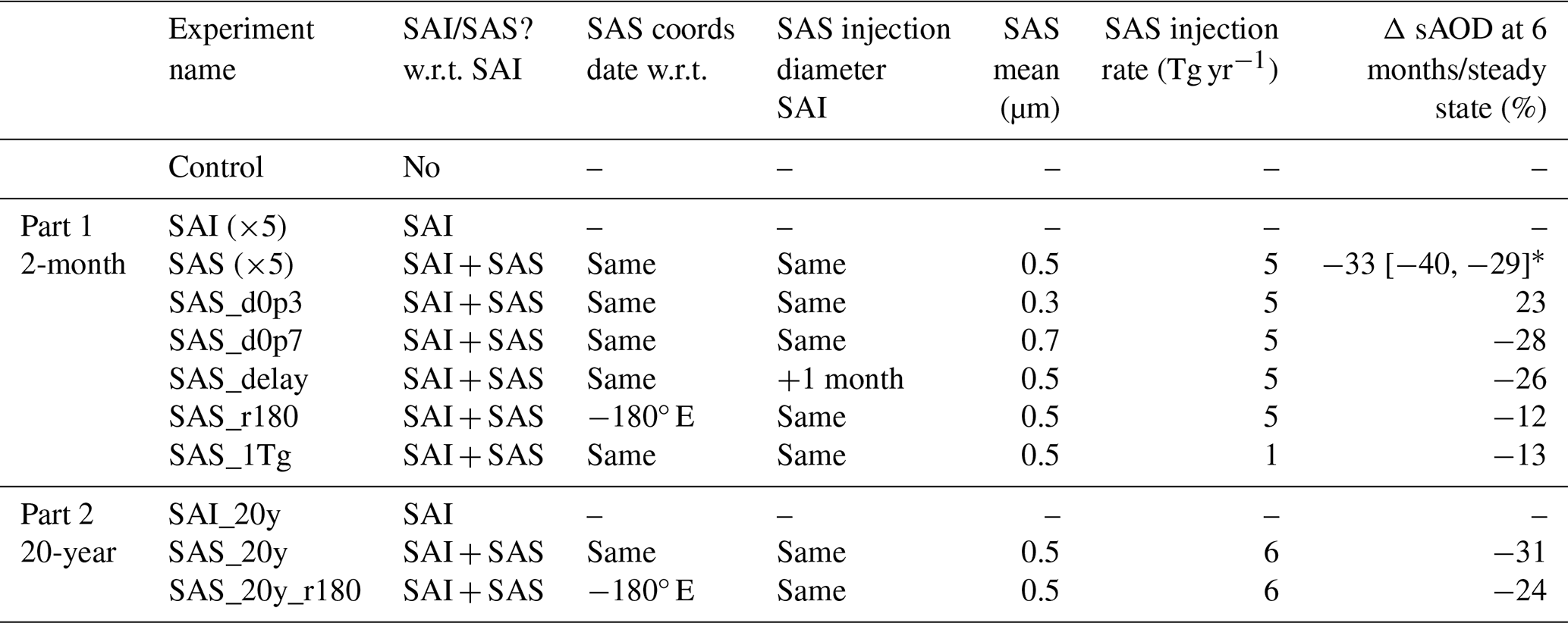
Table 1 Simulation design. The Control and Part 2 simulations are run for 20 years from 1 September 1988. The Part 1 simulations are initialised from 1 Juni 2003 and run for 5 years apart. Δ sAOD refers to the stratospheric 550 nm AOD anomaly in the SAS simulations relative to SAI. In the Part 1 simulations, 5 Tg SO₂ is injected over 2 months. In the Part 2 simulations, 12 Tg SO₂ is injected evenly over a year. ^* Values in square brackets show the ensemble range.

2.2 Simulation design

UM-GAL9 simulations are performed using Atmospheric Model Intercomparison Project (AMIP) protocol, and with CMIP6-defined historical greenhouse gas and aerosol emissions and concentrations. Sea-surface temperature and sea-ice fields are the time series from the NOAA high-resolution blended analysis of daily sea surface temperature (SST) and ice (OISST V2) reanalysis product (Reynolds et al., 2007) and are updated daily. The simulations are free-running with the “Control” simulation run for 20 model years in total (1 September 1988–1 September 2008).

Details of the simulations are provided in Table 1. We perform 2 sets of simulations: (Part 1) two month “pulse” SAI/SAS deployments to explore the sensitivity of atmospheric aerosol lifetime decay to different SAS strategies; (Part 2) 20-year “sustained” simulations with continuous SAI/SAS to explore the steady state impact. For the pulse interventions, we explore sensitivity to SAS deployment region (comparing SAS co-located and offset by 180° longitude with SAI); SAS injection rate (5 or 1 Tg calcite); SAS deployment date (either simultaneous deployment with SAI or 1 month delayed from the SAI deployment); and the size of the injected calcite (either 0.3, 0.5, or 0.7 µm median diameter with a fixed width of σ=1.1 resembling a monodisperse aerosol distribution). Preliminary simulations with injection of larger calcite particles (1 and 5 µm) produced no tangible impact on sAOD at 550 nm due to rapid sedimentation of the calcite particles and are not shown here.

For the Part 1 simulations, we use a single baseline SAI scenario in which 5 Tg SO₂ is emitted evenly from 1 June 2003–1 July 2003 in a latitude-longitude box with edges 20-30° W and 5° S–5° N and between 18–22 km altitude. It is important to note the simplicity of the SAI design which mirrors early SAI simulations, with strategies selected to mirror large tropical volcanic eruptions like Mt Pinatubo in 1991 (e.g. Jones et al., 2016b). In the last decade, the SAI scenario design space has increased in complexity with the application of control theory to optimize injection strategies (e.g. GLENS, Tilmes et al., 2018). Our approach represents a sub-optimal SAI strategy, but due to the position of injection over the Equator and within the lower stratosphere, aerosol spreads globally via the Brewer-Dobson circulation producing a well-distributed aerosol cloud albeit one with a peak in the tropics (Jones et al., 2017). Table 1 breaks down all simulations performed in this study. For statistical robustness, 4 extra ensemble members are run for the “SAI” and “SAS” simulations, with the extra members commencing from 1 June 1991, 1 June 1994, 1 June 1997, and 1 June 2000 time slices in the Control simulation.

For the Part 2 simulations, we inject 12 Tg yr⁻¹ of SO₂ in the same region as for Part 1 ([20–30° W, 5° S–5° N] between 18–22 km altitude) for the entire duration of the 20 yr AMIP simulation spanning 1 September 1988–1 September 2008. We then emit 6 Tg yr⁻¹ calcite in 2 different regions – coincident with SO₂ (region 1) and at −180° longitude offset (region 4). Only a single ensemble member is run for each simulation, and only the last 15 years are used for analyses to allow the stratospheric aerosol fields to attain a pseudo steady state. The injection rate of 12 Tg(SO₂) yr⁻¹ is significant and is approximately equal to 1 Mt Pinatubo eruption per year (Quaglia et al., 2023).

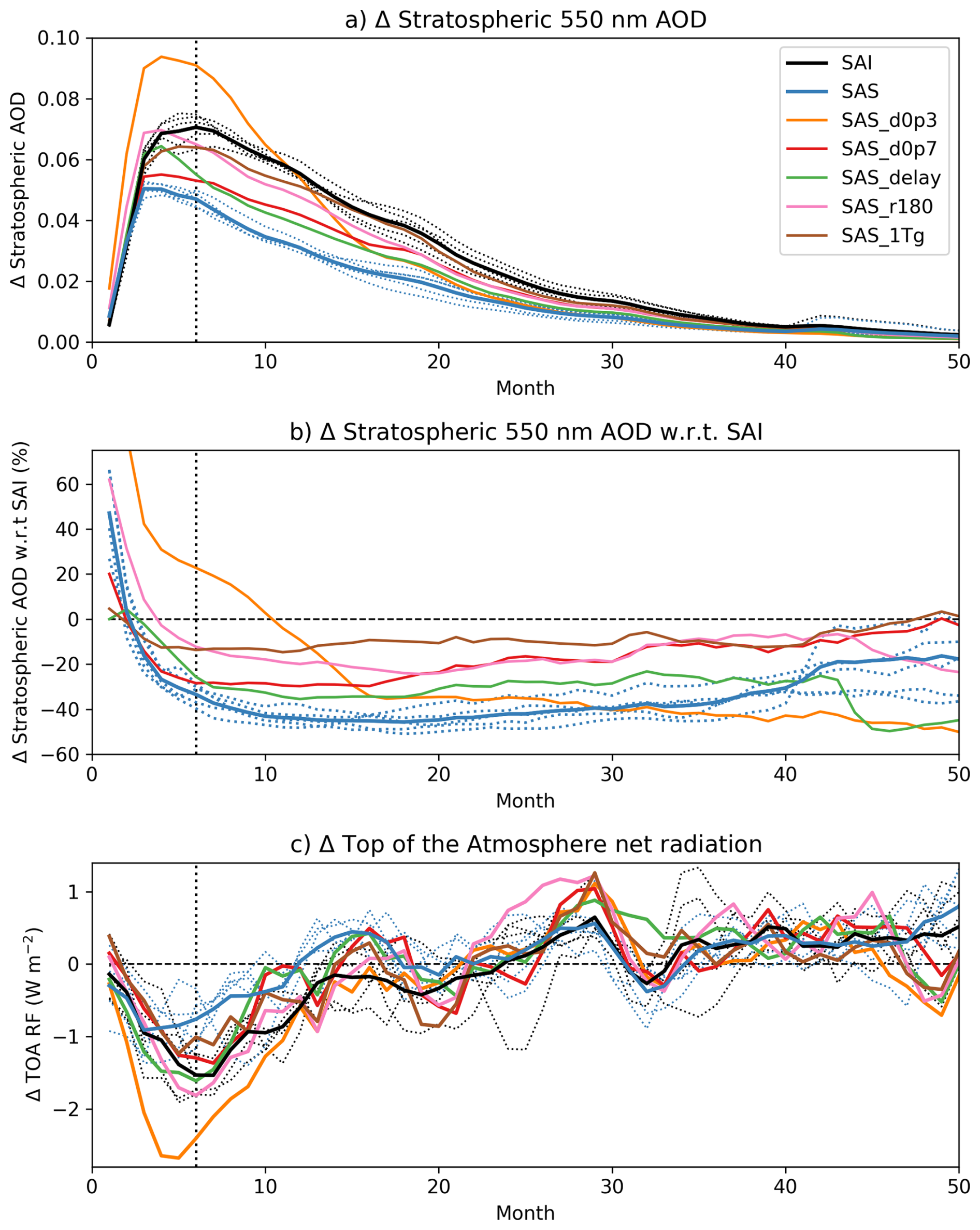
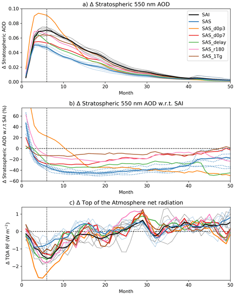
Figure 1 Global mean anomalies: (a) Stratospheric Aerosol Optical Depth (sAOD) at 550 nm anomaly in the Part 1 simulations with respect to control; (b) % difference between SAS and SAI stratospheric AOD anomalies. Dotted lines are used for ensemble members with thick lines of the same colour for the ensemble means. The control SAOD over this period is 0.0005±0.0003 (1 SD). (c) Accumulated global energy budget from integrating top of the atmosphere radiative flux anomalies from the start of the simulation onward.

3 Results

3.1 Part 1: Single-month interventions

In Part 1, we simulate SAI and SAS pulse interventions, investigating sensitivity to aerosol size, delay, injection rate, and region. Figure 1a, b shows the global sAOD anomaly, where sAOD is proportional to the extinction efficiency and mass of radiatively active aerosol and is useful to quantify impacts on radiation and global cooling. The sensitivity simulations show an optimal sAOD reduction with calcite particles with 0.5 µm diameter (“SAS”). In “SAS” the peak sAOD offset at month 6 in the first ensemble member relative to “SAI” is −39 %, which can be compared to +23 % for 0.3 µm (“SAS_d0p3”) and −28 % for 0.7 µm (“SAS_d0p7”). This suggests that a suboptimal SAS strategy may exacerbate rather than neutralise the impact of SAI. At 0.3 µm, calcite's effective diameter is close to the peak solar wavelength and so calcite is acting as a sunlight reflector (Ferraro et al., 2011). While the first “SAS” ensemble member shows a −39 % change in peak sAOD, the ensemble mean change is −33 % demonstrating ensemble variability in the response (−40 % to −29 %).

If SAS is delayed by 1 month (“SAS” vs. “SAS_delay”) then peak sAOD perturbation is reduced from −39 % to −26 % suggesting that SAS may still be effective even for a delayed intervention. If 1 Tg rather than 5 Tg calcite is injected (“SAS_1Tg”), peak sAOD changes by −13 % which indicates that SAS would be less effective with a smaller calcite injection mass. Lastly, SAS with injection at −180° longitude relative to SAI (“SAS_r180”) has a smaller impact of −12 % sAOD perturbation suggesting that for a pulse SAI intervention, SAS would be more effective in closer proximity to SAI. Sensitivity to the emission region will be explored more in the Part 2 simulations. “SAS” has a significant impact on global top-of-the-atmosphere net radiative flux (ToA_RF calculated by summing solar and terrestrial energy perturbations), reducing the net impact of “SAI” at 6 months from −1.53 to −0.76 Wm⁻² although note the significant variability in this metric (Fig. 1c).

Our results are conditional on the use of a single ensemble member and do not factor in meteorological variability which is important for stratospheric aerosol transport (Jones et al., 2016b). For the rest of this section, we explore the differences between “SAI” and “SAS”, with the larger response in “SAS” compared to other sensitivity simulations providing clearer results for a process-level analysis, and with 5-member ensembles providing statistical robustness.

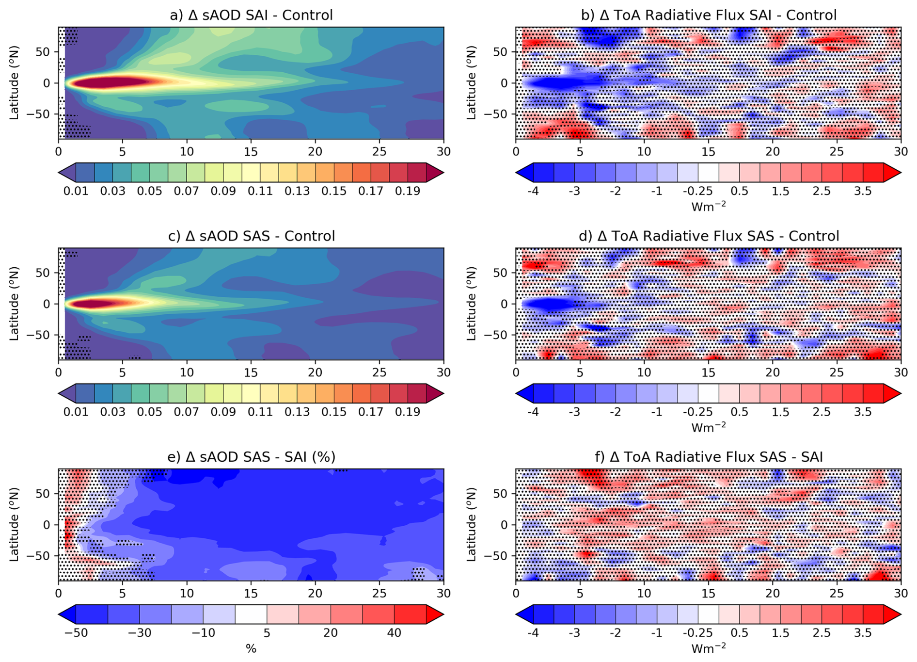
Figure 2 Zonal-mean vs. time plots of (left) Stratospheric Aerosol Optical Depth (sAOD) and (right) Top of the Atmosphere (ToA) net radiative flux anomalies in the 5-member ensemble simulations: SAI and SAS vs. the control simulation. (bottom row) difference between SAI and SAS. Hatching indicates where differences are insignificant at the 5 % level using a paired t-test.

Figure 2 shows the time evolution of sAOD and ToA_RF for the “SAI” and “SAS” simulations relative to the “Control”. The sAOD evolution in “SAI” is very similar to the sAOD evolution following Mt. Pinatubo (Quaglia et al., 2023) with initial containment of aerosol in the tropical pipe and intermittent aerosol transport to higher latitudes primarily during the hemispheric Spring seasons. Before month 5, differences in sAOD and ToA_RF between “SAI” and “SAS” are insignificant with the tropical aerosol augmented to reach a peak sAOD of ∼ 0.3. From month 6, the difference in sAOD increases rapidly with the tropical sAOD anomaly reduced by 40 %–50 % by month 8 in “SAS”. Globally, for the 30-month period following intervention, the net ToA_RF anomaly in “SAI” is −0.38 Wm⁻² comprising a SW forcing of −0.51 Wm⁻² and a LW forcing of +0.13 Wm⁻², and in “SAS” is −0.06 Wm⁻² comprising a SW forcing of −0.14 Wm⁻² and a LW forcing of +0.08 Wm⁻².

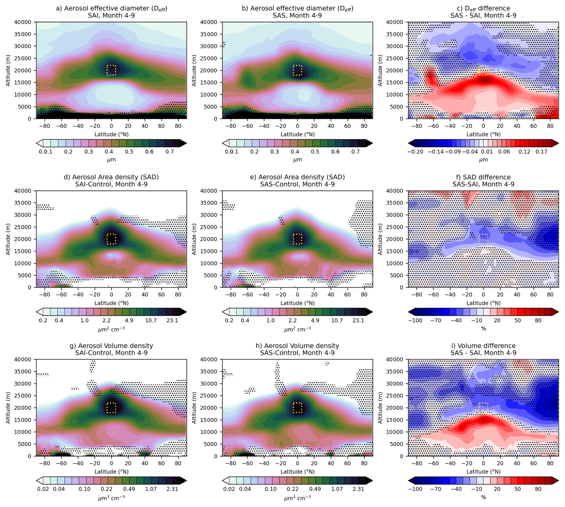
Figure 3 Zonal-mean vs. altitude plots of (top) aerosol effective diameter, (middle) aerosol surface area-density, and (bottom) volume density for: (left) SAI, (middle) SAS_5Tg and (right) differences (raw for diameter, percentage for area and volume). The quantities are integrated over the soluble aerosol modes between months 4 and 9 (Sep Year 1 – Feb Year 2) after the simulated intervention. The aerosol injection region is highlighted by a yellow box. Hatching indicates where differences are insignificant at the 5 % level using a paired t-test.

Figure 3 shows the zonal-mean aerosol effective diameter, surface area density (SAD), and volume density averaged between months 4 and 9 following the start of the intervention. The peak stratospheric SAD and volume are contained to the tropics. The peak tropical SAD of ∼ 20 µm² cm⁻³ in “SAI” is similar to the peak SAD following the 1991 Mt. Pinatubo eruption of ∼ 25 µm² cm⁻³ (Fig. 9 in Quaglia et al., 2023). This is despite emissions of only 5 Tg SO₂ in these simulations with 15 Tg SO₂ emitted by Mt Pinatubo. The coincidental comparability of the SAD between “SAI” and the Mt Pinatubo observations is most likely due to the different SO₂ emission durations, with 2 months in our simulations and ∼ 1 d for the eruption, and thus the greater spread of aerosol in the “SAI” simulation should reduce aerosol growth and lead to a longer atmospheric lifetime.

Aerosol SAD and volume density are consistently 30 %–40 % less in “SAS” than in “SAI” across the lower-to-middle stratosphere (Fig. 3f, i), with the largest differences of 80 % seen at the Northern Hemisphere pole. The aerosol volume is also increased by 70 %–80 % directly below the tropopause in the tropics and extratropics (Fig. 3i). The aerosol effective diameter is larger by ∼ 0.2 µm along isentropic surfaces below the altitude of injection, suggesting that the vertical transport of aerosol in “SAS” is partially inhibited and that larger aerosol is transported by the lower branch of the Brewer Dobson circulation through which it is more readily mixed into the troposphere (Buchart, 2014). Interestingly, aerosol at higher altitudes in the tropics and in the polar regions, is smaller by up to 0.1 µm under “SAS” (Fig. 3c), owing to diminished coagulation as less H₂SO₄ is transported upward (see Fig. 5).

Figure 4 shows (Fig. 4a) the global SO₂, H₂SO₄ and calcite burden anomalies and (Fig. 4b–f) maps of accumulated aerosol deposition anomalies. Combined, these metrics describe the lifetime of atmospheric aerosol and where it is eventually removed from the atmosphere. “SAS” has limited impact on the SO₂ atmospheric decay rate but significantly reduces the e-folding H₂SO₄ lifetime from 15.4 months to 10.2 months, suggesting that calcite does not expedite overall condensation rate (which affects SO₂ lifetime) but promotes growth into larger internal mixtures of calcite/H₂SO₄ aerosol particles more susceptible to sedimentation. The H₂SO₄ deposition anomaly-maps show large regional variations which can probably not be solely attributed to SAS/SAI H₂SO₄ (Fig. 4b–d). However, the calcite deposition indicates that SAS aerosol is preferentially deposited in the tropics to extra-tropics with significant deposition over land regions and limited deposition over the poles.

We now interrogate these simulations to identify the processes which control the aerosol concentrations and allow SAS to counteract SAI. Figure 5 decomposes aerosol process rates for months 1–2 and 3–8 of the “Control”, “SAI” and “SAS” simulations. In months 1–2, SAS reduces condensation onto the Aitken (−29 kg s⁻¹) and accumulation (−168 kg s⁻¹) modes, instead promoting condensation onto coarse aerosol (+177 kg s⁻¹). Additionally, coagulation between the coarse calcite and other modes is significant in “SAS” (+159 kg s⁻¹) and becomes more important than condensation in months 3–8 as the SO₂ reservoir is depleted. We infer that SAS intervention contemporaneous to SAI produces a larger effect than a delayed response because of the increased availability of coarse condensation nuclei in the former. If SAS misses the SO₂ reservoir window, it relies primarily on coagulation rather than condensation to produce the desired growth effect.

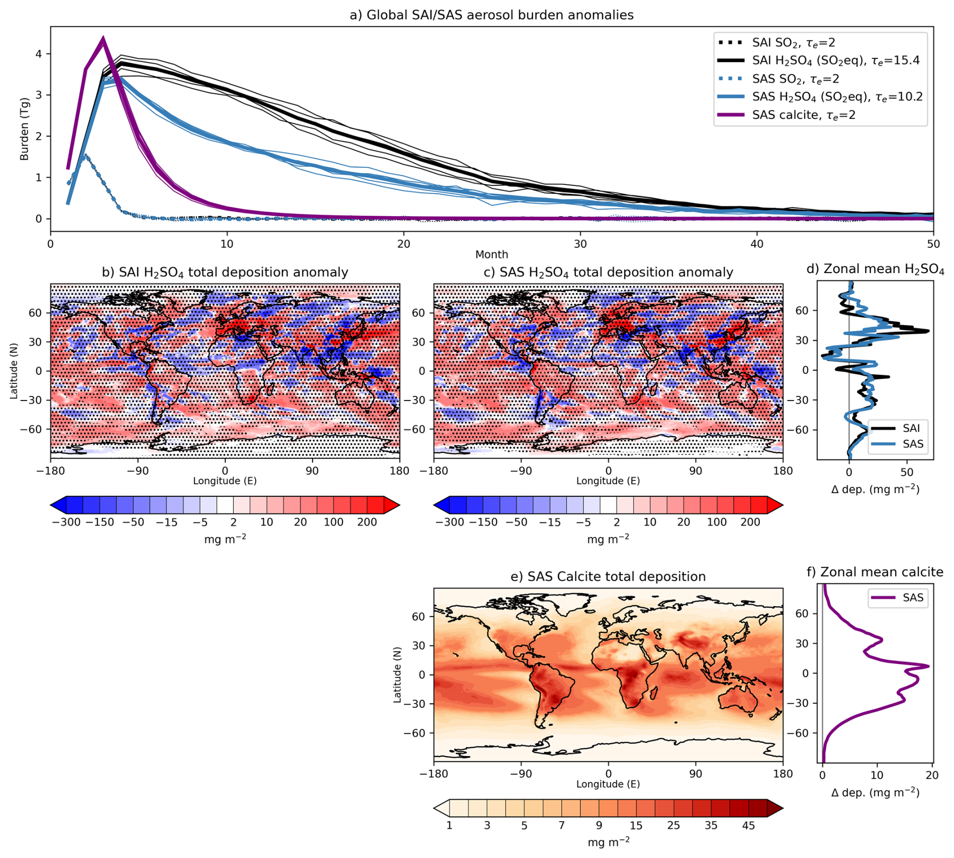
Figure 4 (a) Global SO₂, H₂SO₄, and calcite atmospheric burden anomalies in SAI and SAS. (b, c) Accumulated H₂SO₄ deposition anomaly in the SAI and SAS simulations relative to the control and (d) zonal means. (e) Accumulated calcite deposition anomaly in SAS and (f) zonal mean. Hatching indicates where differences are insignificant at the 5 % level using a paired t-test.

3.2 Part 2: Sustained interventions

In the Part 2 simulations, we inject 12 Tg SO₂ per year in the same region as for “SAI” in the Part 1 simulations. SAS is emitted at a rate of 6 Tg calcite per year, either co-located with SAI (“SAS_20y”) or on the opposite side of the world (“SAS_20y_r180”). Figure 6 shows the global mean sAOD, ToA_RF, and aerosol burden anomalies. Equilibrium conditions are effectively reached after 5 years; we perform much of our analyses omitting the 5 year spin up. The equilibrium sAOD anomaly is reduced by 31 % and 24 % in the `SAS' and “SAS_r180” simulations respectively, in alignment with the Part 1 simulations. This is despite the SAS calcite mass being half of the SAI SO₂ mass in the Part 2 simulations and equal in the Part 1 simulations. This demonstrates a clear difference between the pulse and sustained effects of SAI/SAS and indicates a continued aerosol growth in the sustained intervention simulations (Niemeier and Timmreck, 2015). The difference in SO₂ and calcite burdens between the experiments is minimal (∼ 0.7 and 2 Tg respectively), but H₂SO₄ is reduced from 11.6 Tg (SO₂eq) in “SAI_20y” to 7.7 and 8.4 in Tg in “SAS_20y” and “SAS_20y_r180” respectively. This corresponds to an average atmospheric lifetime of 0.97, 0.65 and 0.71 years in “SAI_20y”, “SAS_20y”, and “SAS_20y_r180” which is comparable to 0.90 ± 0.019 in other equatorial SAI simulations with UKESM1 (Henry et al., 2024).

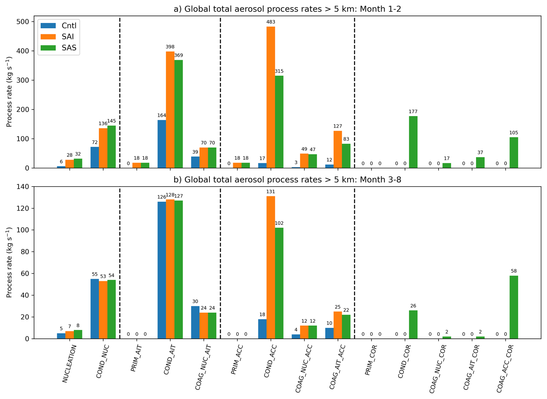
Figure 5 Total aerosol process rates for (a) during SAI/SAS deployment (months 1–2), and (b) the 6 months after deployment (months 3–8) in the Control, SAI, and SAS simulations. Quantities are integrated above 5 km altitude. We neglect intra-mode coagulation which will also contribute to aerosol growth.

Figure 7 shows the zonal mean aerosol effective diameter, SAD and volume density in the “SAI_20y” simulation and differences in the SAS simulations. In “SAI_20y”, the aerosol volume and SAD is concentrated near the injection region with significant concentrations across the lower stratosphere (Fig. 7i). The aerosol grows to attain a steady-state effective diameter of 0.7–0.9 µm across the stratospheric aerosol layer under SAI (Fig. 7a). In the “SAS_20y” simulation, aerosol diameter and volume are enhanced directly below the injection region, suggesting that larger aerosol is removed in the tropics (Fig. 7b, j). A similar response is seen in “SAS_20y_r180” but with less aerosol growth and removed volume (Fig. 7c, k). In general, “SAS_20y_r180” displays a similar steady-state aerosol perturbation to “SAS_20y” but of smaller magnitude.

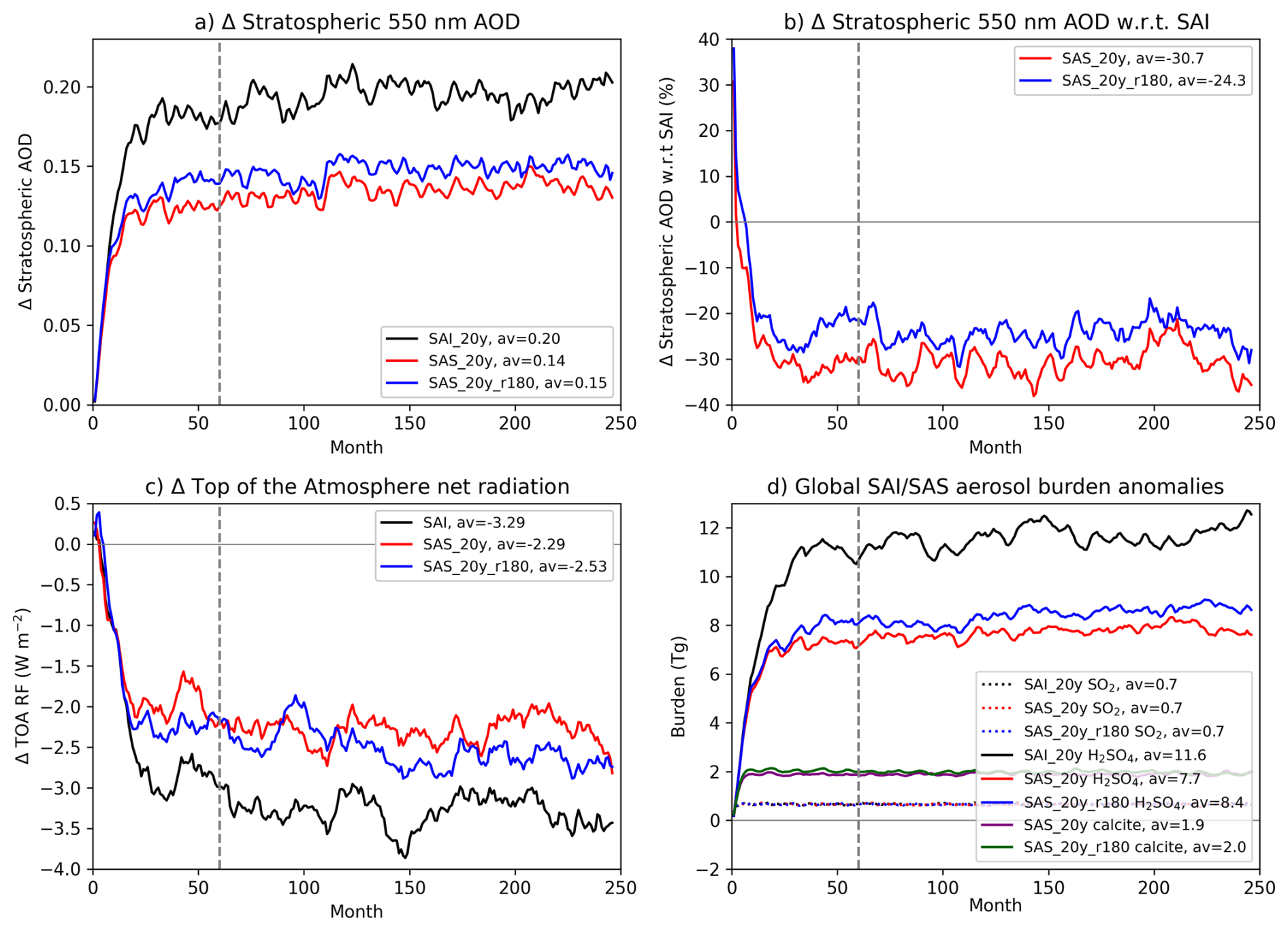
Figure 6 Global-mean anomalies in the Part 2, 20y simulations: (a) sAOD anomaly with respect to Control; (b) sAOD anomaly in the SAS simulations with respect to SAI; (c) Top Of the Atmosphere (TOA) net radiation anomaly; and (d) SO₂, H₂SO₄ (SO₂ eq) and calcite burden anomalies. The ToA_RF anomalies in (c) are smoothed by a 12-month running mean.

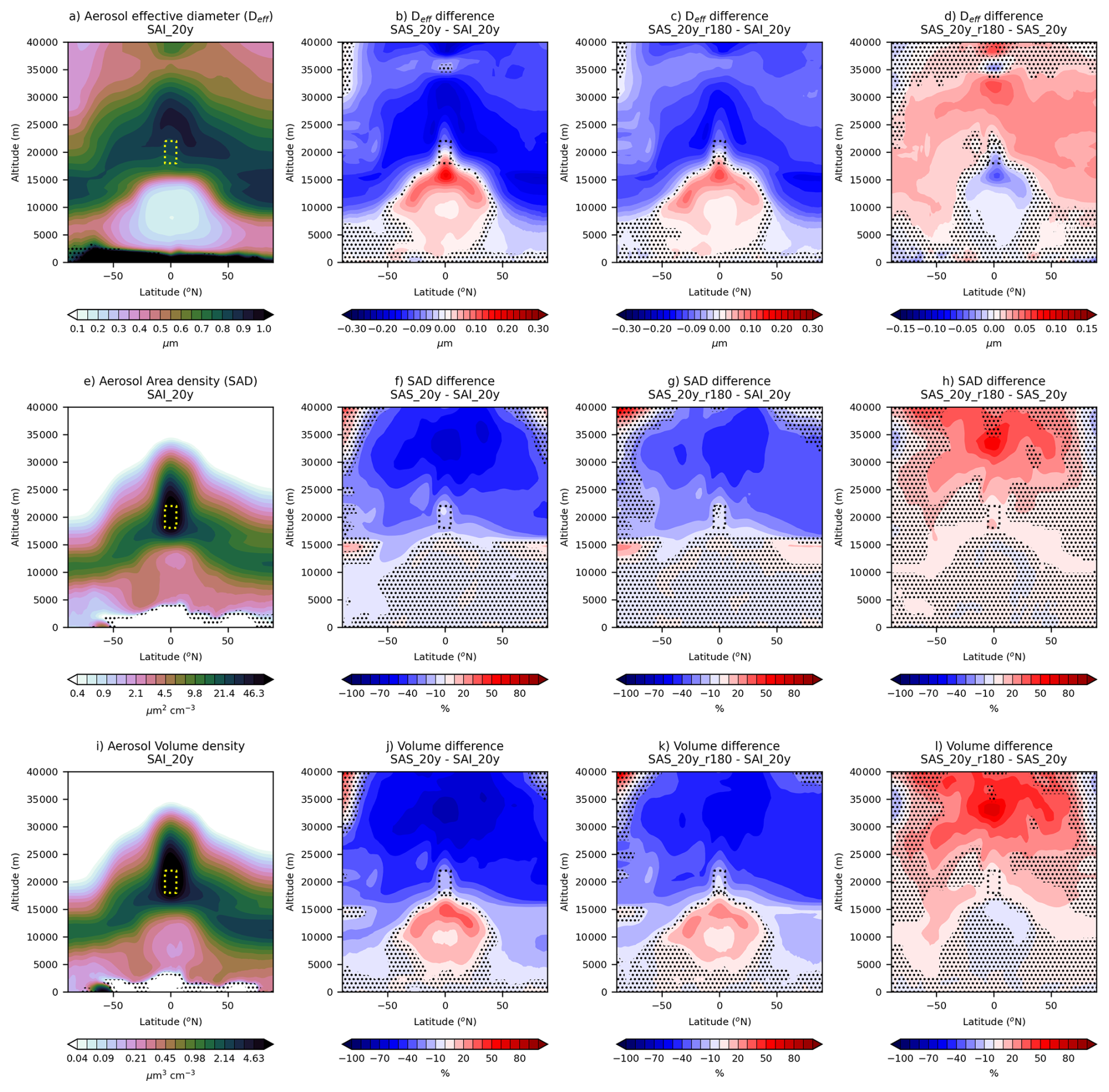
Figure 7 Zonal-mean vs. altitude plots of (top) aerosol effective diameter, (middle) aerosol surface area-density, and (bottom) volume density for: (a, e, d) SAI_20y, (b, f, j) SAS_20y minus SAI_20y, (c, g, k) SAS_20y_r180 minus SAI_20y, and (d, h, l) SAS_20y_r180 minus SAS_20y (raw differences for diameter, percentage for area and volume). The quantities are integrated over the soluble aerosol modes using annual means for the final 15 simulation years. The aerosol injection region is highlighted by a yellow/black box. Hatching indicates where differences are insignificant at the 5 % level using a pooled t-test.

Aerosol deposition anomalies are much larger in the sustained interventions (Fig. 8) than in the pulse simulations (Fig. 4) owing to the greater injection mass. This allows us to fully deduce the distribution of aerosol deposition above the natural noise. In the “SAI_20y”, “SAS_20y”, and “SAS_20y_r180” simulations, a clear pattern of zonal aerosol deposition emerges with peaks over the Equator, extra-tropics (e.g. Himalayas) and decreasing toward the poles (Fig. 8d). SAS preferentially deposits H₂SO₄ near the Equator injection region compared to SAI, which concomitantly reduces the deposition rate between 40–70° N. We infer that SAS would enhance aerosol deposition rates closer to the injection region.

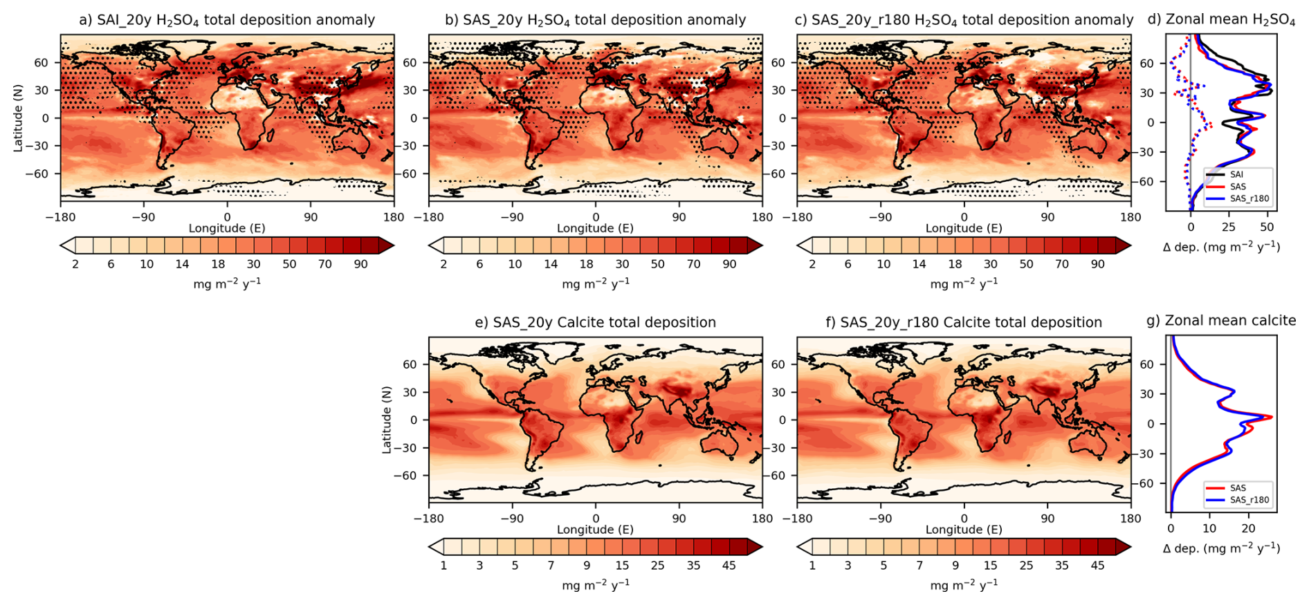
Figure 8 (a, b, c, e, f) Regional H₂SO₄ and calcite deposition rate anomalies in the Part 2 simulations for the last 15 simulated years and (d, g) zonal means. The dashed lines in Fig. 9d indicate SAS anomalies with respect to SAI. Hatching indicates where differences are insignificant at the 5 % level using a pooled t-test.

Analogously to Part 1, we perform a process-level analysis to understand the differences between the “SAS_20y” and “SAS_20y_r180” simulations in Fig. 9. Aerosol process rates are integrated above 5 km altitude for the (a) 5-year spin up and (b) 15-year equilibrium period. The results are qualitatively the same for the 2 periods, with the biggest differences between the simulations being condensation onto the accumulation mode (a greater reduction in “SAS_20y” than “SAS_20y_r180”) and condensation onto the coarse mode (a greater increase in “SAS_20y”). The inter-mode coagulation rates are consistent between the 2 simulations suggesting that the largest difference is in the availability of coarse aerosol for SO₂ condensation which is much greater in “SAS_20y”. Therefore, SAS appears to be more effective as condensation nuclei in an SO₂-rich plume rather than facilitating coagulation between existing particles.

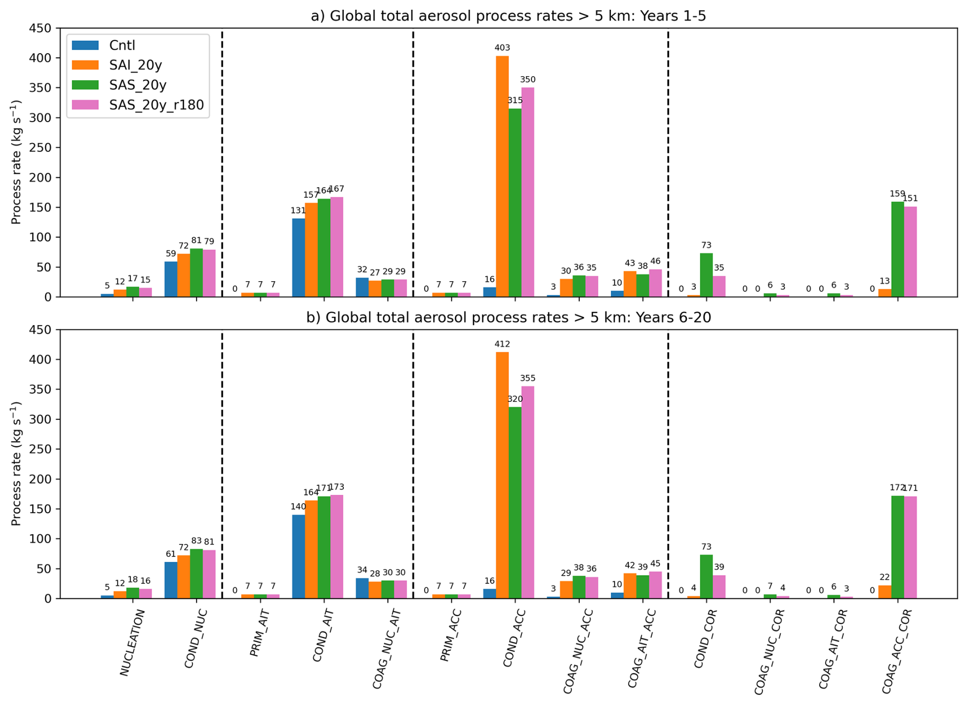
Figure 9 Total aerosol process rates in part 2 simulations for (a) during the spin-up period (Years 1–5), and (b) the equilibrium period (years 6–20) in the Control, SAI_20y, SAS_20y and SAS_20y_r180 simulations. Quantities are integrated above 5 km altitude.

4 Discussion

We explore a Counter Climate Intervention method which we term “Stratospheric Aerosol Scrubbing” (SAS) given its similarity to Flue Gas Scrubbing. We simulate scenarios of Stratospheric Aerosol Injection (SAI) and SAS with the UM-GAL9 model and evaluate the efficacy of SAS using suitable aerosol and radiation metrics. We find that SAS reduces the global aerosol burden, stratospheric Aerosol Optical Depth (sAOD) and net radiative flux anomalies by ∼ 30 % when equal mass of calcite to SO₂ is injected in pulse interventions and half the mass of SO₂ is injected in sustained interventions. We show that SAS promotes condensation and coagulation onto the larger particles, which then sediment rapidly via lower pathways of the stratospheric circulation.

Our results are conditional on the scenario design, meteorological conditions, and model details. For this investigation, we inject into a small region on Earth's equator (5° S–5° N, 30–40° W, 18–22 km altitude). As with early SAI experiments, this “zero-dimension deployment” is to take advantage of stratospheric dynamics, with the Brewer Dobson circulation transporting the aerosol poleward and aerosol persisting for multiple years (Butchart, 2014). However, the design space for SAI is increasingly complex and other SAI backdrops could be evaluated for SAS efficacy in future, for instance injecting aerosol at higher latitudes and at lower stratospheric altitudes (Duffey et al., 2025). For the pulse simulations, we commence interventions in June in a nod to the 1991 Mt Pinatubo eruption, but this is an arbitrary design choice which should be tested in future studies for seasonal dependence. We use a climate-resolution model, albeit one which in previous configurations (with exactly the same representation of aerosol microphysics) has been used for volcanic eruption assessments (Zanchettin et al., 2022) and SAI experiments (Wells et al., 2024) and shown to have good skill in representing stratospheric dynamics and aerosol evolution compared to post-volcanic observations (Wells et al., 2023). Our decision to simulate idealized SAS applications in the recent historical period rather than utilize GeoMIP scenarios as a basis is motivated by the state of readiness of UM-GAL9, which is an updated atmospheric configuration of UKESM1. In a future study, we will explore more realistic SAS applications using CMIP7-era GeoMIP scenarios as a basis allowing for a wider comparison with other climate models.

The representation of calcite in UM-GAL9 is simplified and omits heterogeneous chemical reactions which change the condensation uptake rate of stratospheric vapours such as nitric acid (HNO₃), hydrochloric acid (HCl), and H₂SO₄ onto the aerosol surface (Vattioni et al., 2024a,b; Cziczo et al., 2019). These simulations therefore represent condensation onto stratospheric calcite in a simplified manner, assuming an uptake coefficient of gaseous H₂SO₄ onto soluble aerosol of 1 as is standard for UKCA-mode. Another simplification of our approach is that UM-GAL9 uses “offline oxidants” chemistry which precludes a full impact assessment of SAS on stratospheric ozone which would require interactive stratospheric chemistry (Bednarz et al., 2025). Only a few models exist with fully interactive stratospheric chemistry, 3-D atmospheric dynamics and sectional aerosol microphysics schemes (Kleinschmitt et al., 2017; Tilmes et al., 2023). The UM relies on a modal aerosol scheme which may not represent aerosol coagulation processes between calcite and sulfate aerosol with as much fidelity as more complex sectional aerosol schemes (e.g. Laakso et al., 2022). Based on these caveats, our results should be interpreted with caution given uncertainty in the representation of processes, the dependence on one climate model, and sensitivity of results to the scenario design. Clyne et al. (2021) found that differences in model physics and chemistry caused significant differences in volcanic aerosol evolution for multi-model simulations of the Mt Tambora eruption. The use of offline rather than online oxidants may overestimate the oxidation rates of SO₂ to form H₂SO₄, as found by Clyne et al. (2021). Given that we show the condensation effect to dominate over coagulation (e.g., Fig. 9), this could imply that SAS efficacy is understated in our simulations. In their laboratory study, McGrory et al. (2022) found that silica and alumina particles continued to grow due to condensation in a sulphur rich environment despite coating effects. Laboratory studies would provide useful constraints to test future SAS modelling studies in the absence of natural analogues.

Given the results of our investigation, we propose running further SAS simulations incorporating models with detailed aerosol microphysics including state-partitioning and heterogeneous chemistry which would help constrain SAS efficacy (Vattioni et al., 2024a, b). Laboratory-based measurements of oxidised SO₂ uptake on calcite or other scrubbing agents as a function of diameter, humidity and ambient acidity provide microphysical constraints. Additionally, the evolution of calcite particles in an aircraft wake could be effectively simulated using controlled laboratory or field experiments or plume modelling to understand how agglomeration may impact the emitted calcite particle size distribution. We have tentatively shown that SAS is sensitive to aerosol size (Fig. 1) and our results indicate that particles with a median diameter of 0.5 µm would be optimal for SAS for pulse simulations. This interesting result should be constrained with more ensemble members and utilising a more detailed aerosol microphysics scheme.

The reduction to lifetime of H₂SO₄ aerosols in both the pulse- and sustained simulations differs from the results of Wells et al. (2024), who included concurrent injection of volcanic ash as well as SO₂ in simulating the eruption of Raikoke in 2019. Wells et al. find an enhancement of the H₂SO₄ lifetime owing to a strong initial radiative heating by the ash leading to a lofting of the H₂SO₄, reducing the exchange of aerosol from the stratosphere into the troposphere. These differences are likely to be due to two primary factors; (i) ash was assumed to be strongly absorbing in the solar region of the spectrum leading to significant lower stratospheric heating, (ii) ash was assumed to be an external mixture with H₂SO₄ and microphysical processes such as condensation of SO₂, and coagulation between H₂SO₄ and ash did not occur. Our simulations suggest some fundamental deficiencies in treating aerosols as external mixtures.

We have performed sensitivity simulations where SAS is co-located and antipodal with SAI. We find that co-located SAS allows rapid condensation onto the coarse aerosol particles suggesting that efficacy decreases with increasing distance from the SAI region but that SAS may be partially effective with remote applications. We have also explored the consequences of SAS delayed by 1 month and shown that this remains partially effective at reducing peak sAOD, albeit less effective than contemporaneous deployment (−26 % compared to −39 %). This preliminary exploration of the SAI-to-SAS proximity domain in effect makes different assumptions on the readiness of an SAS actor to begin “scrubbing” and its areal proximity to the original SAI application. One area that we do not explore is performance of SAS in a mature, well-spread SAI aerosol layer. For example, if SAI were started, continued for multiple years, and then immediately ceased, how effective would SAS be in facilitating stratospheric aerosol removal and returning Earth to a baseline climate? There is another dimension to our results which we have hinted at which is the potential for SAS to offset the impacts of a super-volcanic eruption in a manner analogous to short-lived greenhouse gas injection (Fuglestvedt et al., 2014). There would likely be greater appetite for SAS than countervailing strategies such as short-lived greenhouse gas injection due to the inherent complexity of the latter (PA18), and a study that directly investigates the efficacy of SAS to offset the cooling effects of a super-volcanic eruption in a similar manner to Fuglestvedt et al. (2014) is warranted.

We have evaluated two intervention scenarios – a pulse intervention that closely resembles a sizable volcanic eruption and a sustained intervention that resembles standard SAI strategies that aim to impose a steady-state multi-year global cooling. These scenarios span a small portion of the temporal SAS design space but should be extended to consider intermediate interventions of between 2 months and 20 years, and SAI scenarios which tailor emissions strategy based on optimal seasons, altitudes and latitudes (Tilmes et al., 2018). Such studies could be informed by online game-theory models in which actors react to the actions of other actors, simulating the geopolitics which may govern SAI and SAS deployments (Heyen et al., 2019).

Although we have tailored our aerosol injection rates to be within the range of the SAI literature, it is pragmatic to consider the technical viability of delivery to the stratosphere. Smith (2020) provide a breakdown of costs associated with SAI and include calcite given that it has been considered as an SAI substrate (Keith et al., 2016). They find that alongside SO₂ and compared to other minerals; calcite is on the cheaper end of the substrate spectrum. For 5 Tg of calcite as injected in the Part 1 simulations, the cost of mining, processing and storing combined can be estimated at USD ∼ 600 million: based on mining costs of USD 10 t⁻¹, ultrafine grinding of USD 100 t⁻¹, and storage of USD 12.5 t⁻¹ yr⁻¹ and assuming storage of a year. The much greater cost is in delivery to stratospheric altitudes, for which novel aircraft would be required (Smith, 2020). Assuming aircraft with a payload of 25 t⁻¹/flight (Smith and Wagner, 2018) and conservatively allowing each aircraft 3 flights per day, injection of 2.5 Tg of a substance per month would require 100 000 flights and a fleet of ∼ 1100 aircraft, exceeding large existing commercial fleets such as FedEx or UPS of < 700 aircraft. This suggests that while theoretically feasible, delivery of 2.5 Tg/month of a substance as in the Part 1 simulations is not yet practically feasible without significant outlay, perhaps requiring 2 decades to develop infrastructure (Smith, 2024). Delivery of 0.5 Tg/month as in the Part 2 simulations would require ∼ 220 aircraft which is much more plausible. Commercial aircraft could be adapted to inject SO₂ or calcite (Duffey et al., 2025), but such deployments can only reach 13 to 15 km hence may be sub-optimal. Nevertheless, the fact that SAS mirrors SAI in design should mean that any infrastructure designed to deliver SO₂ to the stratosphere could be adapted for SAS, albeit needing specialised nozzles to emit calcite and limit agglomeration (Neukermans et al., 2021).

Whether ∼ 30 %–40 % reduction in aerosol burden due to SAS is “effective”, “partially effective” or “ineffective” is subjective depending on cost-benefit assumptions and it is important to note the high scenario-related uncertainty in the SAS response in our simulations (e.g., Fig. 1). Nevertheless, an SAI deterrent such as SAS could provide an effective barrier against unilateral SAI deployments or the “free rider” problem (e.g., Heyen et al., 2019) which should be factored into this discussion. In summary, we have established using idealized simulations that SAS could be partially effective at counteracting SAI by producing a significant 30 %–40 % reduction in aerosol optical depth and therefore warrants further investigation using more complex aerosol microphysical models and realistic SAI scenarios.