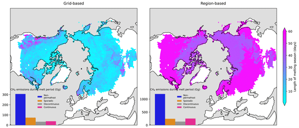
Melt period methane emissions in northern high latitude wetlands are governed by the length of the period and presence of permafrost

Northern high latitude wetlands are significant sources of methane, with emissions driven by seasonal soil freezing and thawing. To better understand the seasonality of northern high latitude methane emissions, we defined the melt period occurring in spring time using the remote sensing Soil Moisture and Ocean Salinity Freeze/Thaw data from 2011–2021. To estimate methane emissions in the northern high latitudes, we used the atmospheric inverse model CarbonTracker Europe-CH₄. The melt period was defined for three permafrost zones and for a seasonally frozen non-permafrost region using two approaches: region-based, which considered climatological conditions of permafrost regions, and grid-based, which defines the melt period at a finer 1°×1° scale.

The length and timing of the melt period varied significantly depending on the approach. The melt period generally occurred between March and June and was influenced by air temperature, with a negative correlation between the length and the mean temperature of the melt period. The longest melt period was in the non-permafrost zone and the shortest varied between the two methods. The melt period emissions were on average 1.83 Tg with the region-based approach and 0.45 Tg with the grid-based approach, the non-permafrost zone having the largest share of the emissions. They were largely dependent on the season’s length. Year-to-year variation was modest, within 15 % (region-based) and 23 % (grid-based) of average emissions, and there was also no trend during the study period. Our dual-method approach allows for robust comparison with both large-scale regional studies and localized site-level research.

1 Introduction

Northern high latitude wetlands are an important and dynamic part of the climate system (Hugelius et al., 2020). They are a large source of methane (CH₄), which is the second most important anthropogenic greenhouse gas causing climate change after carbon dioxide (CO₂) (Forster et al., 2021). It has a 29.8 times stronger global warming potential over a 100 year timescale than CO₂ without considering climate feedbacks. A large portion of the total soil carbon is stored in northern wetlands and the underlying permafrost, containing ∼80 % (415±150 Pg C, Hugelius et al., 2020) of the total global peatland carbon, with nearly half being permafrost affected peatland (Hugelius et al., 2020; Scharlemann et al., 2014). Due to climate change and Arctic amplification, thawing permafrost could affect this carbon stock (Schuur et al., 2015; Knoblauch et al., 2018; Voigt et al., 2019; Turetsky et al., 2020). Even though permafrost thaw will likely lead to soil drying and increased drainage, which potentially accelerates organic matter decomposition and CO₂ emissions while suppressing CH₄ emissions (Lawrence et al., 2015), the effect of the released CH₄ might be as large due to its stronger global warming potential (Schuur and Abbott, 2011). Increasing rainfall and warming soils could increase near-term global warming, and the total annual boreal CH₄ emissions could rise 4 Tg yr⁻¹ (Neumann et al., 2019). The study by Poulter et al. (2017) using a biochemical model concluded that boreal wetland CH₄ emissions have already increased by 1.2 Tg yr⁻¹ between 2000–2012. Even if the permafrost does not fully thaw, the deepening of the active layer  – the top layer of soil that thaws in summer and freezes in winter  – can still release a significant amount of carbon.

In addition to permafrost thaw, Arctic amplification is expected to significantly impact snowmelt and seasonal soil thawing, including the active layer, in northern high latitude wetlands. There are still a lot of open questions related to the future of methane emissions in the northern high latitudes due to uncertainties in the wetness of the area and possible feedback loops. For instance, de Vrese et al. (2023) demonstrated that atmospheric feedbacks resulting from the increasingly dry Arctic may offset the effects of growing wetland extent and result in comparable CH₄ emissions as in the case where the Arctic would remain wet. The changing Arctic hydrology affects the melt period emissions as well (Rawlins and Karmalkar, 2024). The hydrological conditions during the melt period in the northern high latitudes are especially uncertain due to the unreliability in the amount of snow as well as the melting and evaporation of snow. This lack of certainty brings unpredictability to the melt period methane emissions.

CH₄ emissions from the northern high latitude wetlands are low during winter when the soil is frozen and high during summer after the soil has thawed (Aselmann and Crutzen, 1989; Rinne et al., 2018), also depending on the soil temperature and hydrological factors (Rychlik, 2009; Zhu et al., 2013; Turetsky et al., 2008). During the spring thawing, the emissions increase rapidly. Typically, the CH₄ storage is low during the thawing after the dormant cold season, and the CH₄ is released gradually as the soil melts (Raz-Yaseef et al., 2017). However, previous studies have reported large bursts of CH₄ from the wetlands during the spring thawing (Jin et al., 1999; Tokida et al., 2007; Song et al., 2012; Raz-Yaseef et al., 2017), though the reports are scarce with only a few measurement sites and just a few years of flux measurements from before the thawing starts (e.g. winter flux data) (Raz-Yaseef et al., 2017). The springtime bursts of CH₄ have been linked to rain-on-snow events which enhance soil cracking (Raz-Yaseef et al., 2017). However, the frequency and impact of these pulses to spring methane emissions are still highly uncertain. Our research did not focus on these springtime bursts, but that does not negate their existence. We focused on large scale methane emissions in the northern high latitudes.

Previous studies have mostly focused on methane emissions during the growing season while the other seasons, such as the autumn freezing period, winter season and the spring thaw season, has received less attention (e.g. Vourlitis et al., 1993; Sachs et al., 2008; Zona et al., 2009; Parmentier et al., 2011). The regional studies focusing on the spring season, have often defined the timing of the whole spring season simply as certain months, e.g. March, April and May (e.g. Castro-Morales et al., 2018; Ito et al., 2023) or in a case of site-level studies, using site-specific soil temperature measurements (e.g. Zona et al., 2016; Bao et al., 2020; Tagesson et al., 2012; Raz-Yaseef et al., 2017). Using soil temperature to define the soil thawing would be ideal, but reliable soil temperature data is available only from point-wise measurements. Thus, to be able to study the melt period on a regional scale, we need to use a proxy for the soil thawing. In this study, we define the melt period in the spring time using the remote-sensed Soil Moisture and Ocean Salinity (SMOS) soil Freeze/Thaw (F/T) data (Rautiainen et al., 2025). The SMOS F/T data provides daily information of the freezing and thawing state of the soil in the northern high latitudes at a resolution of 25 km. Using the SMOS F/T data gives us a dynamic picture of the soil thawing including the active layer of the permafrost during the spring and enables us to define the melt period for the whole northern high latitude region instead of using a static definition (e.g. specific months). This allows us to focus on the CH₄ emissions during the actual thawing of the soil instead of the whole spring season with inverse modeling. The SMOS F/T data have been used successfully to define summer thaw, autumn freezing, and winter cold seasons in the northern high latitude wetlands (Tenkanen et al., 2021; Erkkilä et al., 2023). In this paper, the SMOS F/T data is used for the first time to define the melt period.

In addition to in-situ measurement based studies, the spring CH₄ emissions have been studied with process-based models (Ito et al., 2023; Castro-Morales et al., 2018). Process-based models estimate methane fluxes by simulating physical, chemical, and biological processes. Another approach to estimate fluxes is inverse modeling. Inverse models are statistical approaches which can be used to inform and “re-evaluate” the process-based estimates and decrease the uncertainties in CH₄ emissions using atmospheric CH₄ measurements, so that the differences between simulations and measurements is minimized (Wittig, 2023).

The aim of this study is to estimate the melt period occurring during the spring season and the corresponding CH₄ emissions in the northern high latitude permafrost and wetland regions. We use the SMOS F/T data to define the melt period and determine methane emissions with the global atmospheric inverse model Carbon Tracker Europe-CH₄ (CTE-CH₄) (Tsuruta et al., 2017) at high spatial resolution of 1° latitude × 1° longitude. The years studied are 2011–2021 due to availability of the SMOS data. Previously, CTE-CH₄ has been used to study northern high latitude wetland emissions for various seasons (Tenkanen et al., 2021; Erkkilä et al., 2023), but this is the first time with a focus on the melt period. The melt period is defined for four different permafrost zones (sporadic, discontinuous and continuous permafrost and a seasonally frozen zone non-permafrost) with a region-based approach, as well as individually for each 1°×1° grid cell with a grid-based approach. For comparison between the two methods to define the melt period, we divided the grid-based melt period into the same four permafrost zones. This allows us to estimate emissions both in climatological and local scales.

2 Materials and methods

2.1 SMOS F/T soil state estimates

To define the melt period of the northern high latitude wetlands, we used the European Space Agency's (ESA) SMOS Soil Freeze and Thaw State product (version 3.0) (Rautiainen et al., 2016; European Space Agency, 2023). The product is derived from observations of the ESA Soil Moisture and Ocean Salinity (SMOS) satellite (Kerr et al., 2010) and provides daily categorical information on near-surface freeze–thaw state at 25 km spatial resolution. The main observational input consists of Centre Aval de Traitement des Données SMOS (CATDS) daily gridded Level-3 brightness temperature data (Al Bitar et al., 2017). Brightness temperature depends on both the physical temperature of the surface and its microwave emissivity. At L-band frequencies, the strong contrast in dielectric properties between liquid water and ice enables sensitivity to near-surface soil freeze–thaw transitions, with partial penetration through vegetation and the upper soil layer. L-band refers to low frequency (1–2 GHz) passive microwave observations (Rautiainen et al., 2025).

The SMOS L3FT retrieval was developed by the Finnish Meteorological Institute in collaboration with GAMMA Remote Sensing, and the full algorithm description and validation are given in Rautiainen et al. (2025). Briefly, the algorithm computes the normalized polarization ratio (NPR) from horizontally and vertically polarized SMOS brightness temperatures, applies filtering and temporal smoothing to the NPR time series, and rescales NPR using grid cell-specific frozen and thawed reference states. These reference states are estimated empirically from multi-year NPR time series using ancillary air temperature and snow information (Rautiainen et al., 2025). The resulting scaled NPR is classified into three soil-state categories using fixed thresholds: thawed (<50 %), partially frozen (50 %–70 %), and frozen (>70 %). Of the three categories, the thawed soil state is used in this study to define the melt period.

Although the SMOS freeze–thaw product is available beyond 2021, we restricted the analysis to the period 2011–2021 to ensure temporal consistency and robust data quality across the study domain. In the later part of the SMOS mission, increasing radio-frequency interference (RFI) has affected observations over Europe and parts of Eurasia. SMOS, as an L-band aperture-synthesis radiometer, is particularly sensitive to RFI, which reduces observation density and degrades retrieval reliability (Oliva et al., 2016; Rautiainen et al., 2025). The SMOS freeze–thaw product is provided separately for ascending (approximately 06:00 LT) and descending (approximately 18:00 LT) satellite overpasses, with operational RFI monitoring indicating orbit-dependent differences in data availability over Europe, the Middle East, and Asia (Uranga et al., 2022). To maximize data quality and spatial coverage, we therefore restricted the analysis to ascending-orbit SMOS observations within the 2011–2021 period.

The SMOS L3 freeze–thaw dataset used in this study is publicly available through the SMOS online dissemination service, with persistent access provided via the dataset DOI (https://doi.org/10.57780/sm1-fbf89e0) (European Space Agency, 2023).

2.2 CarbonTracker Europe-CH₄

The methane fluxes were estimated with the CarbonTracker Europe-CH₄ (CTE-CH₄) inverse model (Tsuruta et al., 2017). In its assimilation phase, a Bayesian cost function was minimized:

$$\begin{array}{}\text{(1)}& \begin{array}{rl}J=& (\mathit{x}-{\mathit{x}}^b{)}^T{\mathbf{P}}^{-\mathrm{1}}(\mathit{x}-{\mathit{x}}^b)\\ & +(\mathit{y}-H(\mathit{x}\left){)}^T{\mathbf{R}}^{-\mathrm{1}}\right(\mathit{y}-H\left(\mathit{x}\right)),\end{array}\end{array}$$

where x is a state vector which contains a set of scaling factors that multiply the prior CH₄ surface fluxes, which are meant to be optimized, and x^b is the prior state vector (see Sect. 2.2.3). P is the state vector error covariance matrix. y is a vector consisting of the atmospheric methane observations (see Sect. 2.2.2) and R is the error covariance matrix of the observations y. H is an observation operator, which is an atmospheric transport model TM5 in this study (see Sect. 2.2.1).

The model used the ensemble Kalman filter (EnKF) (Evensen, 2003; Peters et al., 2005) data assimilation scheme within the CarbonTracker Data Assimilation Shell (CTDAS) (van der Laan-Luijkx et al., 2017) with an ensemble size of 500 and a 5 week lag to optimize the fluxes (Peters et al., 2005; Tsuruta et al., 2017). The anthropogenic and natural fluxes were optimized separately but simultaneously in a weekly temporal resolution. The fluxes in the high northern latitudes were optimized at the spatial resolution of 1°×1°, and regionally elsewhere. The spatial correlation followed an exponential decay model (Peters et al., 2005) with correlation lengths of 100 km for 1°×1° grid-based domains, 500 km for other land domains, and 900 km for oceanic domains. Anthropogenic and natural CH₄ fluxes were assumed to be uncorrelated, as were land and ocean domains.

2.2.1 TM5 chemistry model

TM5 is an atmospheric chemistry transport model (Krol et al., 2005). Here, it was used as the observation operator to transform the methane fluxes to atmospheric mole fractions. In this study, its global horizontal resolution was 4°×6° with an intermediate zoom region of 2°×3° (14–82° N, 36° W–54° E) framing a 1°×1° zoom over Europe (24–74° N, 21° W–45° E). The model used preprocessed meteorological data from ECMWF ERA5 reanalysis data with a 3 h resolution (Hersbach et al., 2020). The vertical domain was divided into 25 hybrid sigma pressure levels from the surface to the upper atmosphere. The chemical loss of CH₄ in the atmosphere to the sinks of OH, was based on monthly precalculated values by Houweling et al. (2014), and Cl and O(¹D) sinks were based on the atmospheric chemistry general circulation model ECHAM5/MESSy1 (Jöckel et al., 2006; Kangasaho et al., 2022). The variability of the atmospheric sinks between different years was not considered, but varied monthly, and the sinks were not optimized.

2.2.2 Observations

In addition to the observations from the ObsPack v4.0 (Schuldt et al., 2021; Masarie et al., 2014), observations from two stations in Finland (Kumpula, Sodankylä) (Tsuruta et al., 2019) and from nine stations in Siberia (Sasakawa et al., 2010, 2025) were used. All stations are listed in the Appendix A1 and the location can be seen in Fig. A1. Globally, 183 stations had observations between 2011–2021, with some stations having two or three institutions contributing. The data included weekly discrete air samples and hourly continuous measurements of CH₄, and the data was filtered according to the institutions' quality flags. Only data points that represented well-mixed conditions were included, which means that daily averages were calculated from 12 to 4 pm LT, except for high mountain sites where averages are calculated from 0 to 4 am LT, following Tsuruta et al. (2017).

Observational uncertainties, or “model–data mismatches”, were estimated for each site based on site-specific factors, measurement accuracy, and the capability of TM5 to simulate atmospheric CH₄ mole fractions (Bruhwiler et al., 2014; Tsuruta et al., 2019). These discrepancies arose from TM5’s resolution and transport errors, with e.g. better performance at remote marine sites compared to those affected by strong local emissions. Sites were categorized, for example, as marine boundary layer (4.5 ppb), terrestrial (25 ppb), mixed marine and terrestrial (15 ppb), and strong local influence (30 ppb). Uncertainties ranged from 4.5 to 75 ppb.

2.2.3 Prior fluxes

The prior anthropogenic emissions were taken from the Emission Database for Global Atmospheric Research (EDGAR v6.0) (Monforti Ferrario et al., 2021). The emissions from LPX-Bern DYPTOP v1.4 (Lienert and Joos, 2018) were used as the natural biospheric prior emissions. Methane emissions from other sources were: Weber et al. (2019) for ocean, the Global fire emission database (GFED v4.1s) (van der Werf et al., 2017; Randerson et al., 2017) for biomass burning, and VISIT (Ito and Inatomi, 2012; Tsuruta et al., 2019) for termites. Biospheric and anthropogenic fluxes were optimized globally. Other fluxes were not optimized. We only analyze the optimized biospheric fluxes in this study. The biospheric prior LPX-Bern DYPTOP represents ecosystem area fractions across several land-cover types: (i) peatlands suitable for peat growth as defined by DYPTOP (Stocker et al., 2014); (ii) rice paddies coinciding with croplands and the presence of rice paddies (Spahni et al., 2011); (iii) inundated wetlands other than peatlands or rice paddies; (iv) wet mineral soils, which are not wetlands, peatlands, rice paddies, permanent freshwater bodies, or ice/sea water covered areas, but are ocassionally wet; and (v) dry mineral soils, which are areas identical to wet mineral soils but are “dry” in general. Of these categories, we did not include rice paddies in our prior as they are not present in the northern high latitude region. Soilsink was included in the biospheric prior.

For both the anthropogenic and biospheric fluxes, we used the prior uncertainty of 80 % for terrestrial fluxes and 20 % for oceanic fluxes, assuming uncorrelated uncertainties, following previous studies (e.g., Tsuruta et al., 2017; Bruhwiler et al., 2014).

2.3 Permafrost map

The permafrost extent (v3.0) is one of the variables belonging to ESA's Climate Change Initiative (CCI) (Bartsch et al., 2020; Obu et al., 2019). The temporal resolution of the data is one year and the spatial resolution is 926.63 m (Obu et al., 2021). Using the permafrost and SMOS F/T soil state data, we split the northern latitudes into four zones depending on how much of the exposed land surface is underlain by permafrost: 90 %–100 % for the continuous permafrost, 50 %–90 % for the discontinuous permafrost, 14 %–50 % for the sporadic zone and the non-permafrost zone mainly comprising areas that were frozen seasonally based on the SMOS F/T data with some potential permafrost spots, since the CCI permafrost data had no values lower than 14 % (Fig. 1). Areas where no SMOS F/T data was available, were excluded from this study. This masking excluded areas such as southern regions below 40° N where almost no permafrost is located, as well as oceans, most of Greenland, and some areas close to the Great Lakes in the USA.

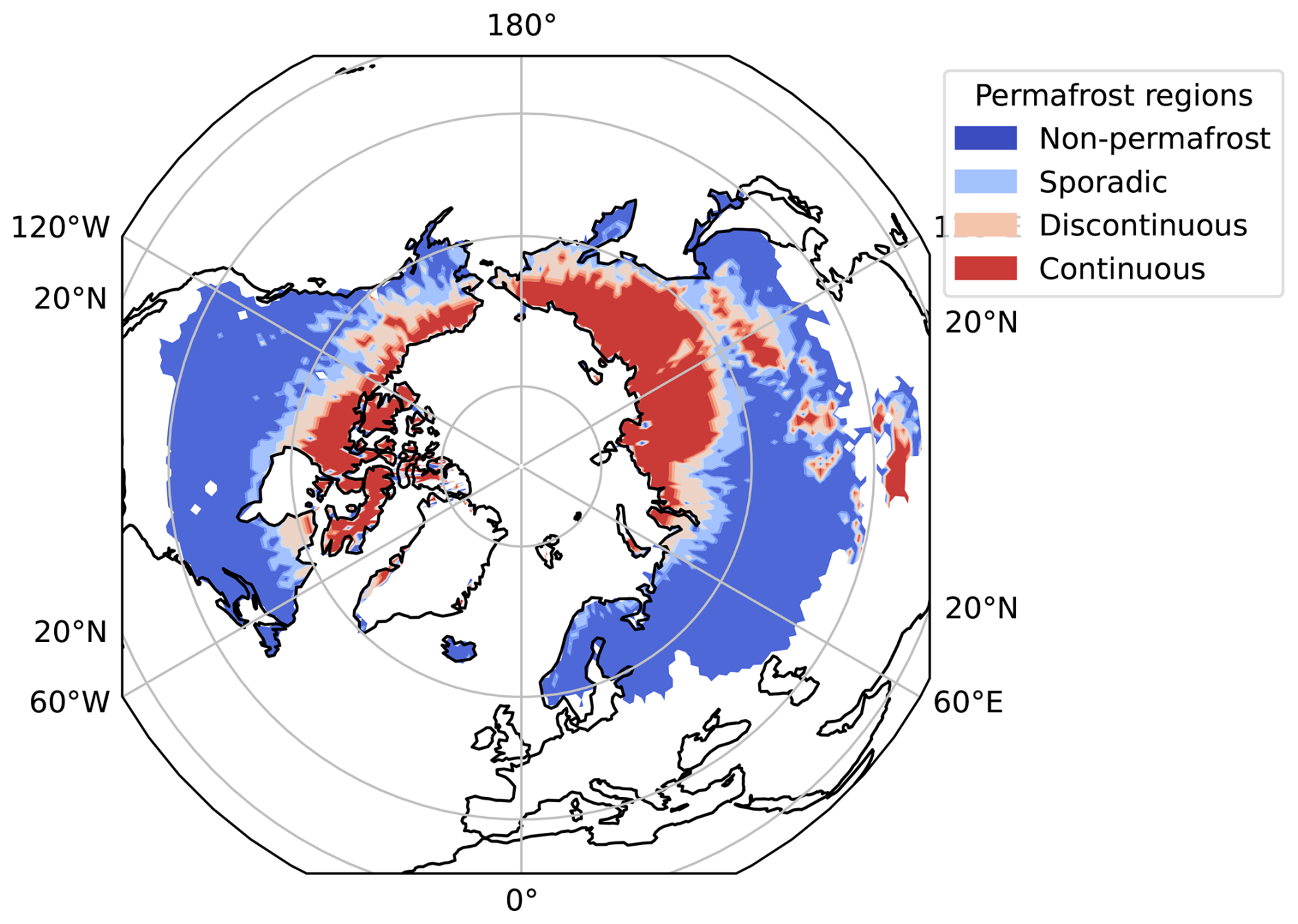
Figure 1 Extents of the four permafrost zones in 1°×1° resolution.

The permafrost data was only available until 2018. Average permafrost zones were calculated from the years 2011–2018. The four permafrost zones had only minor changes between the different years. The permafrost percentage was calculated at a 1°×1° resolution by averaging the original 1 km data within each grid cell. The average areas were used in this study to define the four permafrost zones for all the years from 2011–2021. We are aware that a newer version of the permafrost data (v4.0) including the years 2019–2021 has been published but it was not used in this study (Westermann et al., 2024).

2.4 ERA5 2 m temperature data

ERA5 is the latest global reanalysis from the ECMWF available from 1959 to the present day (, 2020). It provides hourly estimates of multiple land, oceanic and atmospheric climate variables. Here, the ERA5 2 m air temperature reanalysis data was used to study the relationship between the air temperature and CTE-CH₄ emissions during the melt period. The ERA5 temperature data was additionally used as an auxiliary dataset in the SMOS F/T data and as input data in the CTE-CH₄.

2.5 Defining the melt period and its methane emissions

2.5.1 Definition of the melt period

In this study, the melt period was defined as a season in the northern latitudes in spring, when the soil in a specific region turned from frozen to thawed based on the “thawed” state in the SMOS F/T data (see Sect. 2.1). The word “melt” is used here instead of “thaw” because the SMOS F/T data can indicate the melting of the snow instead of the soil, especially at the beginning of the melt period. This is because the microwave radiation signal from wet snow resembles the signal from thawed soil (Rautiainen et al., 2016). However, methane emissions are possible even at the very beginning of the melt period because the air temperature rises above zero and melted or rain water can trickle into the soil and wintertime methane reserves are released (Hargreaves et al., 2001; Rinne et al., 2007; Song et al., 2012; Raz-Yaseef et al., 2017). It is thus justified to start the melt period from the melting of the snow. The boundaries used in this study were similar to the ones used by Erkkilä et al. (2023) to define different seasons in the northern high latitude wetlands, but instead of frozen or partially frozen state of the SMOS F/T data, we used the thawed soil state to define the melt period. The resolution of the SMOS F/T data was changed from 25 km×25 km to 1°×1° by calculating the fraction of the thawed 25 km×25 km pixels whose center was inside the 1°×1° grid cell.

The melt period was defined for four permafrost zones: non-permafrost, sporadic, discontinuous and continuous permafrost (region-based approach), and separately for each 1°×1° grid cell (grid-based approach) in these zones. The region-based approach gives information about the permafrost areas constrained by their specific climatological conditions while the grid-based melt period was studied to illustrate the local variation in the melting of the soil.

With the region-based approach, the melt period was set to start (1) when the mean thawing fraction of a permafrost zone had surpassed the minimum thawing fraction of that year by 0.1 ($\text{thaw}\left(\mathit{\%}\right)\ge {\text{thaw}}_{\text{min,year}}\left(\mathit{\%}\right)+\mathrm{10}\mathit{\%}$), and (2) after the day when the zone reaches its minimum annual mean thawing fraction before mid July. During some years, the freezing of the soil continued past the turn of the year, which meant that the (1) boundary was reached before the maximum freezing of the soil. This meant that the additional (2) condition for the beginning of the melt period had to be defined. With the (2) condition, the melt period could be separated from the autumn freezing period. In regions with permafrost, the first (1) condition was surpassed later during the spring than the second (2) condition, but in the non-permafrost zone the second (2) condition was needed.

The season ended when the mean thawing fraction of the whole zone had surpassed 0.8 of the maximum thawing fraction of all years which was 1 for all zones ($\text{thaw}\left(\mathit{\%}\right)/{\text{thaw}}_{\text{max,all}}\left(\mathit{\%}\right)\ge \mathrm{80}\mathit{\%}$). The fraction of 0.8 was chosen because there was not as much variation in the thawing fraction that close to summer indicating a stable thaw state. The day when the melt period ended was included in the melt period. The melt period in each grid cell was defined from the amount of thawed pixels in a grid cell, emphasizing more the small grid cells in the north. The mean thawing fraction of all grid cells in a permafrost zone was then calculated. The selected thresholds were chosen to define a robust, zone-mean transition period rather than the exact timing of soil thaw at individual grid cells. In early spring, the SMOS F/T signal can respond to wet snow in addition to thawed soil, as liquid water in the snowpack produces a microwave signature similar to that of thawed soil (Rautiainen et al., 2025). Consequently, thawing fractions very close to 0 % or 100 % are more sensitive to short-term fluctuations in the microwave signal. Defining the season boundaries away from these extremes ensures that the melt period reflects a sustained, large-scale transition.

In the grid-based approach, the start of the melt period was defined differently. The season started when (1) one SMOS F/T pixel (25 km×25 km) in the 1°×1° grid cell had melted and (2) after the day when the grid cell reaches its minimum annual thawing fraction before the end of July. The second condition was needed for the same reason as in the region-based approach. There were a maximum of 18 SMOS F/T pixels and a minimum of 1 pixel in each 1°×1° grid cell depending on data availability and geographic location. For example, in a grid cell with 18 pixels, the season started when the thawing fraction was $\mathrm{1}/\mathrm{18}$, meaning that 5.6 % of the area of that grid cell has melted. The season ended when the thawing fraction in the grid cell had surpassed 0.8 of the maximum thawing fraction of that year. To separate the spring melt period from the autumn freezing season, the melt period was defined to start and end before the 212th day of the year (end of July). Missing data in the grid cells was replaced by interpolating linearly between the previous and the coming day with an existing value. If none of the pixels melted in a grid cell, or if the thawing fraction never was below 0.8 of the maximum thawing fraction of that year before the end of July, meaning that the grid cell did not freeze, the grid cell did not have a melt period. In some of the grid cells, the condition for the end of the melt period was never surpassed before the 212th day of the year even though the season had a beginning. For those grid cells, the end of the melt period was defined as a day when the soil had thawed the maximum amount during the melt period. However, this only happened in 2 grid cells in 2017. Additionally, in a few grid cells, the minimum thaw fraction occurred after the maximum had already been reached. In these cases, the onset of the season was defined to occur prior to the maximum. Excluding the first three years, fewer than 1 % of grid cells in the study area did not have a melt period annually. In the first three years, this percentage ranged from 6.5 % in 2011 to 1.1 % in 2013.

2.5.2 Calculating melt period methane emissions

After defining the melt period, the methane emissions were calculated from the CTE-CH₄ inverse model biospheric posterior emission estimates. The methane emissions were optimized weekly, and to calculate the daily emissions, the model data was interpolated linearly from one optimized weekly value to the next weekly value. From these daily values, the posterior methane emissions were analysed during the melt period. Similarly to the melt period, the regional emissions were calculated separately for the four permafrost zones: non-permafrost, sporadic, discontinuous and continuous permafrost zones.

The total melt period CH₄ emissions in a region or grid cell in teragrams of methane (Tg CH₄ per region per season, hereafter denoted simply as Tg) were calculated from the daily methane emission estimate. The daily values of all grid cells were added together in each permafrost zone during the melt period. The average emissions were calculated in the unit of $\mathrm{\mu }\mathrm{g}{\mathrm{CH}}_{\mathrm{4}}{\mathrm{m}}^{-\mathrm{2}}{\mathrm{s}}^{-\mathrm{1}}$ by dividing the average daily emissions during the melt period in a permafrost zone by the area of the specific permafrost zone. The emissions were studied against the land area of the permafrost zones instead of the actual area of wetlands or permafrost in each zone. This was done because the exact area of wetlands is uncertain (Saunois et al., 2025), and using the estimated wetland area extent would have added another source of uncertainty.

As the melt period was defined separately for each 1°×1° grid cell, the melt period emissions were calculated separately as well. The sum of the emissions per grid cell per melt period was calculated in each grid from the first day of the melt period to the last. To calculate average of the methane emissions in the unit of $\mathrm{\mu }\mathrm{g}{\mathrm{CH}}_{\mathrm{4}}{\mathrm{m}}^{-\mathrm{2}}{\mathrm{s}}^{-\mathrm{1}}$, the average daily emissions during the melt period in a grid cell were divided by the respective area of the grid cell. To compare with the other method, we divided the grid-based emissions to the four permafrost regions as well.

3 Results

3.1 Length of the melt period

The average length of the melt period over all the permafrost zones was approximately four times longer when the region-based approach (45 d) was used than when the grid-based approach was used (10 d) (Fig. 2). Using the grid-based approach, the average length of the melt period was the longest in the southernmost zone, non-permafrost (12 d), and the shortest in the northernmost zone, continuous permafrost (7 d) (Figs. 2–4). For the region-based melt period, there was no as clear gradient in the north–south direction as there was in the grid-based mean lengths. However, the longest melt period was typically still in the southernmost permafrost zone, the non-permafrost (57 d), except for 2011, when the longest season was in the continuous permafrost zone (54 d), and in 2018, when it was the longest in the sporadic zone (57 d). On average, the region-based season was the shortest in the sporadic and discontinuous zones (40 d), which also had smaller areas than the other two zones. The years with the longest and shortest melt periods differed between the two methods and grid-based and region-based lengths of the melt period also did not strongly correlate (Fig. A2).

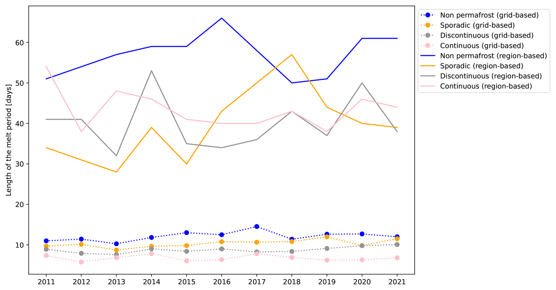
Figure 2 The length of the melt period defined with the two methods in the northern high latitude permafrost zones. The dotted lines represent the grid-based mean length of the melt period. The solid lines represent the region-based melt period.

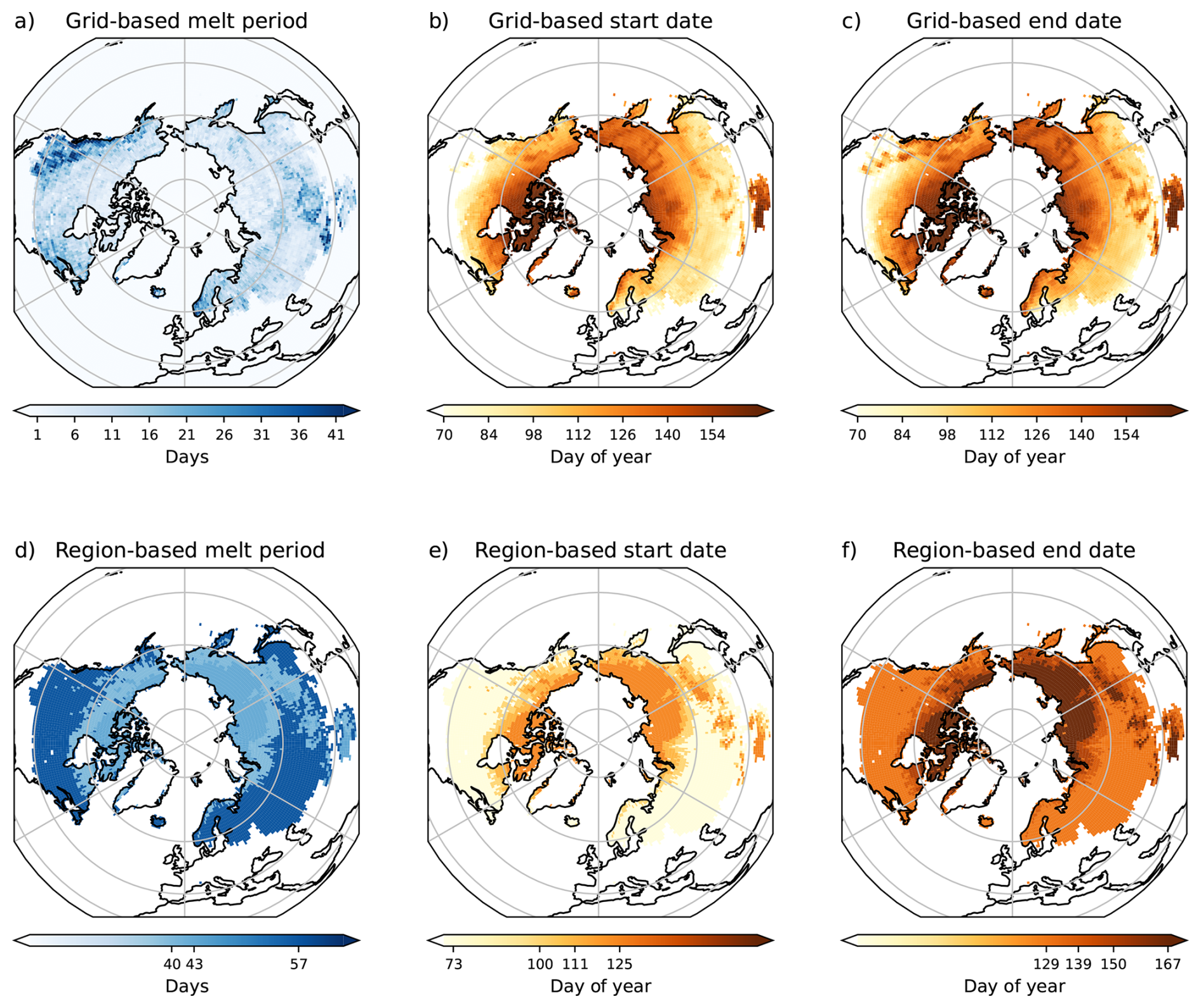
Figure 3 Grid-based (panels a–c) and region-based (panels d–f) average length, start day, and end day of the melt period in the northern high latitudes, averaged over 2011–2021. Notice the different color-range in the melt period panels on the left side (a, d). In the region-based panels, only the illustrated length, start and end days are ticked on the color-bar. The color range in the start and end day panels are the same in the grid- and region-based panels.

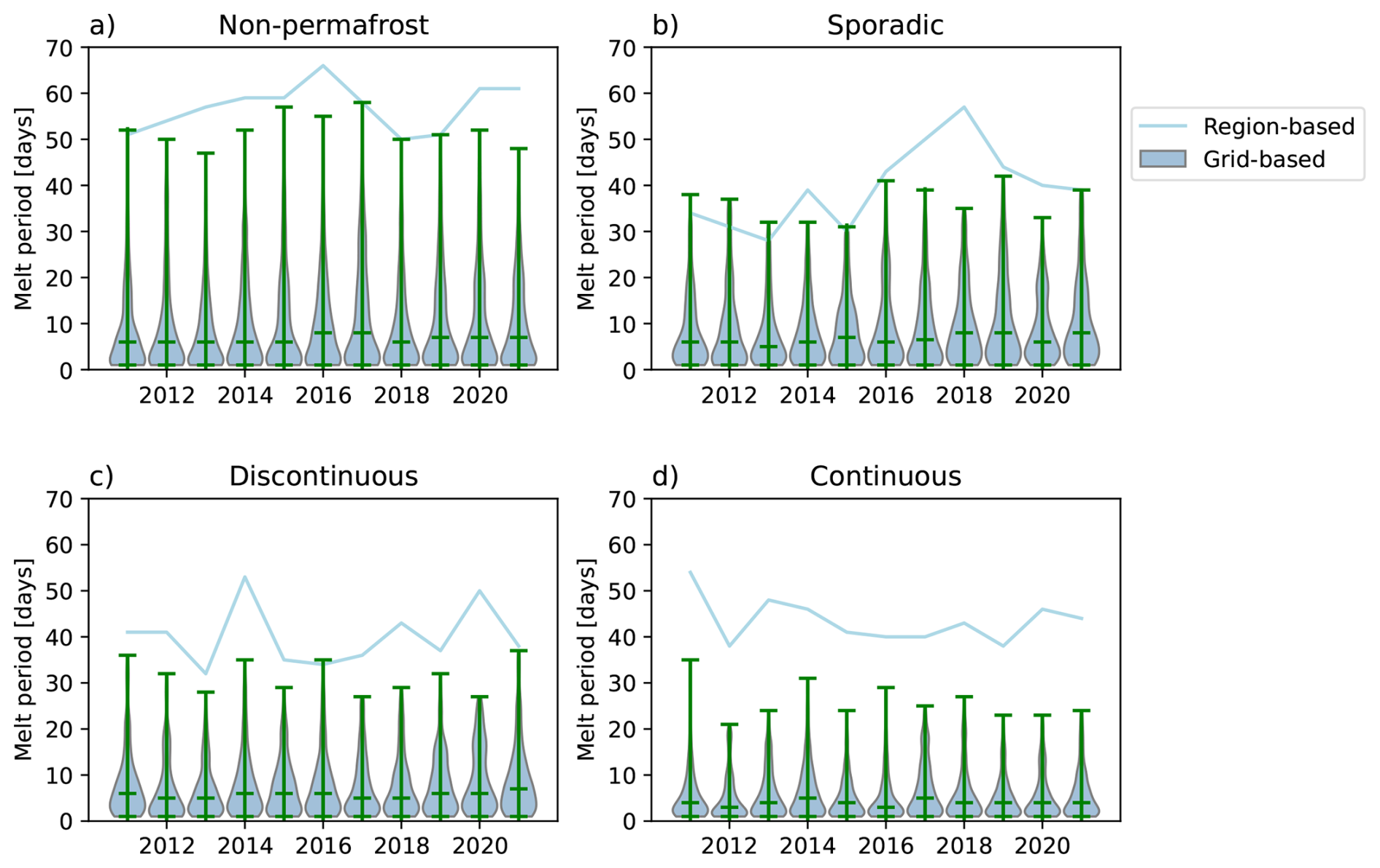
Figure 4 The length of the melt period defined with the two methods in the northern high latitude zones: (a) non-permafrost, (b) sporadic, (c) discontinuous and (d) continuous permafrost. The violin plots represent the grid-based length distribution in the four zones. The medians as well as the min and 97.5 percentile max values for each year are shown as well with the green lines. Grid cells where the length of the melt period was longer than the 97.5 percentile were not included. The blue lines represent the region-based length of the season.

Most of the of grid-based melt periods lasted only a few days (Fig. 4). However, some grid cells had a very long melt period, some as long as the region-based melt period. For example, the West Coast of Canada and the USA had large areas with a longer melt period (Fig. 3). Other areas with a noticeably longer melt period include the coast of Norway, Iceland, East Coast of the USA, Mongolia, the southern parts of Russia and Northern China. The shortest melt period in a grid cell was one day in all the zones and the longest season was found in the sporadic zone and it lasted 212 d, the length of the the maximum duration of the melt period based on our method. It was clearly an outlier, since 95 % of grid cells in the sporadic zone had a melt period season shorter than 31 d. In addition, 95th percentiles for other zones were 40 d in the non-permafrost zone, 26 d in the discontinuous permafrost zones, and 20 d in the continuous permafrost zone. From Fig. 4 we can see the gradient in the north–south direction of the longest (97.5 percentile) grid-based melt periods, with the longest melt periods on average in the southernmost zone, non-permafrost (Fig. 4a).

With the region-based approach, the length of the melt period had a larger inter-annual variation (7–17 d depending on the permafrost zone) than the average length of the grid-based season (Fig. 2), which might be linked to the inter-annual variations of climate in the permafrost zones, as the region-based method focuses more on the climatological averages. Hence, the grid-based method is better at detecting the actual melting of the snow and soil on a local level, because it detects the faster changes in a specific grid cell. An example of inter-annual variation of weather affecting the region-based length of the melt period is in 2011, when in the continuous permafrost zone, the average ERA5 2 m mean air temperature was the lowest and the melt period was the longest. In contrast, in 2017 and 2019, the 2 m mean temperature was higher and melt period shorter in the continuous permafrost zone. In 2013, the spring melt period was the shortest in the sporadic and discontinuous permafrost zones. According to the ERA5 2 m air temperature data, the melt period mean temperature was higher in these two zones than during other years of our study period. In 2015, the mean temperature on these two zones was higher during the spring melt period as well. This suggest that the melt period was shorter and warmer after the colder weather surpassed. In 2017–2019, the sporadic zone had its longest melt period while the mean temperatures were the lowest. This all indicates that the melt period timing and length were linked to the mean temperature of the zone.

The longer melt period in the southern regions could have been caused by an early onset of the melt period, followed by variation between negative and positive temperatures, which would have slowed down the melting. The early onset of the melt period and the consecutive variation between temperatures would have made the mean temperature lower and the melt period longer. To confirm this, the relationship between the length of the melt period and mean temperature was studied (Fig. 5). A negative correlation was found between the two variables, which was the strongest in the discontinuous permafrost zone (region-based p=0.008) and sporadic zone (grid-based p=0.005). With the region-based approach, the correlation between the variables was significant (p<0.05) for all the zones and there was a more prominent negative correlation between the length and the starting day of the melt period in all the permafrost zones (p<0.001 for all the zones, Fig. A3). This indicates that the later the season started, the shorter the melt period was, at least in the larger permafrost zone scale. Additionally, there was a positive correlation between the region-based starting day of the melt period and the mean temperature of the melt period (sporadic: p<0.001, continuous: p<0.01, and non-permafrost and discontinuous: p<0.05). This all indicates that the melt period started earlier, when the mean temperature was lower, on a larger scale.

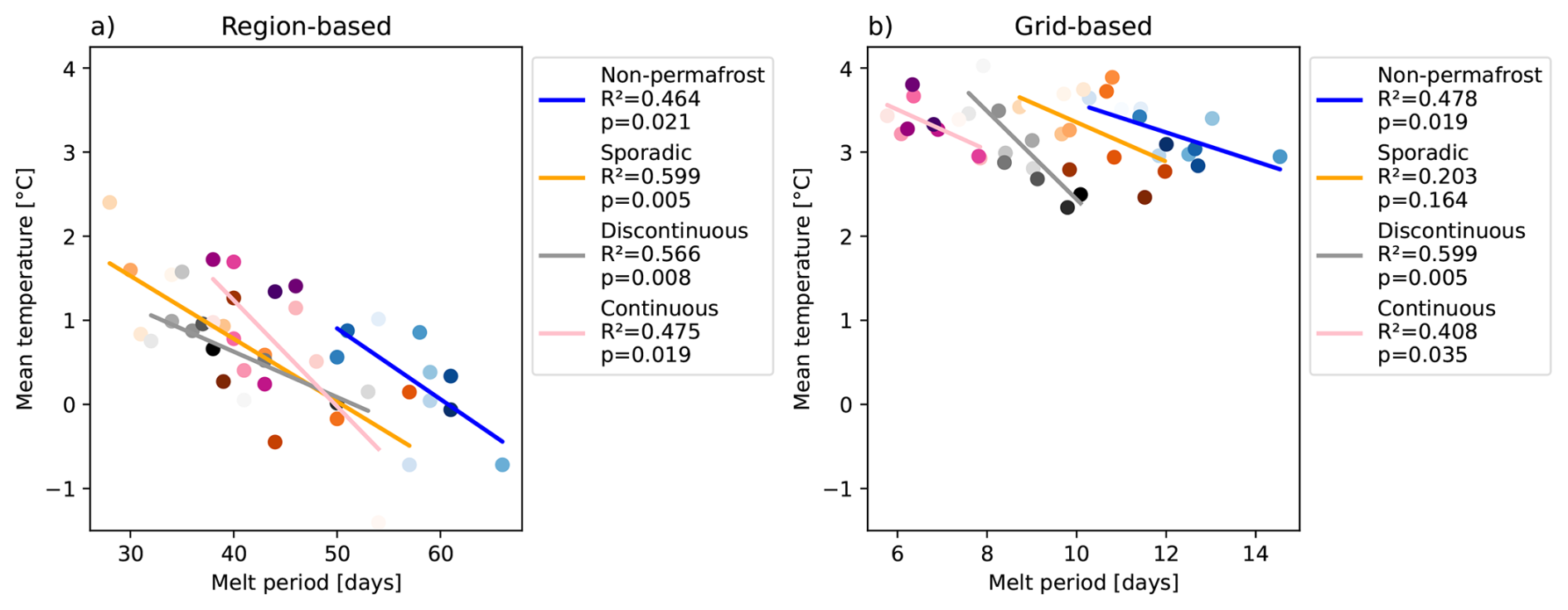
Figure 5 Panel (a) depicts the region-based relationship between the length of the melt period and the mean temperature of the melt period. Panel (b) depicts the grid-based relationship between the mean length and the mean temperature of the melt period. The scatter plot color gradient represents the different years with 2011 being the lightest color and 2021 being the darkest. R² and p in the legends are the coefficient of determination and p-values of the slopes from linear regression fit, indicating statistical significance of the coefficient of determination.

With the grid-based approach there was not as strong a correlation between the mean starting day of the melt period and the mean temperature or mean length of the melt period (p≥0.1 for most of the permafrost zones). Additionally, the melt period mean temperature was higher with the grid-based approach than with the region-based approach (Fig. 5). Looking at the individual grid cells could have given a different output. The mean values of the length, temperature and starting day of the grid-based melt period may be insufficient to describe their relationship because the variation between different grid cells is not seen.

3.1.1 Start and end days of the melt period

With the region-based melt period, the start and end of the season varied from year to year in each permafrost zone (Table A2). The range of variation of the starting days was 21 d in the non-permafrost and sporadic zones, 15 d in the discontinuous permafrost zone, and 18 d in the continuous permafrost zone. The range of variation of the ending days was shorter, only 6 d in the non-permafrost zone, 14 d in the sporadic zone, and 8 d in the discontinuous and continuous permafrost zones. Between different grid cells, the start and end of the melt period varied more within a year than the averages from year to year. However, even inside one grid cell, there was more inter-annual variation that was not seen from the average (Fig. A4b and c). On average, the region-based melt period started earlier and ended later than the grid-based melt period. However, in some grid cells, the melt period started much earlier and ended later than the region-based season, as expected since at least 10 % of the grid cells had to be thawed for the region-based melt period to start and 80 % had to be melted for it to end.

With both methods, the season typically started and ended the earliest in the southernmost regions and the latest in the northernmost regions, with the season starting later in some of the southernmost grid cells (mostly mountainous regions). Using the grid-based approach, the melt period in the southernmost regions began as early as January. However, the average onset occurred in April in the non-permafrost zone and in May in the continuous permafrost zone, although the earliest onset in the latter was already observed in February. Similarly, the melt period ended earliest in January in the non-permafrost zone and in March in the continuous permafrost zone. On average, the season ended in April in the non-permafrost zone and in June in the continuous permafrost zone. Using the region-based approach, the melt period in the non-permafrost zone extended from mid-March to early May. In the sporadic permafrost zone, it lasted from mid-April to mid-May. In the discontinuous permafrost zone, the season began in the second half of April and ended in late May. In the continuous permafrost zone, the melt period occurred from early May to mid-June. In the Eurasian continent, the melt period started earlier in the west and later in the east. The regions with the most permafrost are located in the eastern part of Eurasia which means that the regions with less permafrost started to melt first. In the American continent, an east–west thawing gradient is not apparent. However, the melt period started and ended the latest where the most permafrost is located. Our region-based melt period started on average 10–20 d earlier in all the zones compared to the start of the thaw season defined by Erkkilä et al. (2023). With our grid-based approach the melt period started on average 1–10 d later than the thaw season.

3.1.2 Melt period in the Hudson Bay lowlands and the Western Siberian lowlands

The melt period was additionally studied in the Hudson Bay lowlands (land area in 50–60° N latitudes and 75–96° W longitudes) and the Western Siberian lowlands (land area in 52–74° N latitudes and 60–94.5° E longitudes). Hudson Bay lowlands and Western Siberian lowlands are some of the largest methane emitting wetlands in the northern high latitudes (Pickett-Heaps et al., 2011; Umezawa et al., 2012). They consist of the four permafrost zones, except the Hudson Bay lowlands where there is no continuous permafrost. On average, the grid-based melt period was slightly shorter in the Western Siberian lowlands (∼9 d than in the Hudson Bay lowlands (∼10 d). The season started and ended a few days earlier on average in the Western Siberian lowlands than in the Hudson Bay lowlands. The region-based melt period length was not defined separately for these wetland regions, but the original region-based lengths in the four permafrost zones were used.

Overall, in the Hudson Bay lowlands, there was a negative correlation between the mean temperature and mean length of the melt period (p<0.05 in all zones) with the grid-based approach. In the Western Siberian lowlands, there was also a negative correlation in all of the permafrost zones but it was statistically significant only in the non-permafrost and sporadic zones (p<0.05). This means that the season was shorter when the mean temperature was higher at least with the grid-based approach.

With the region-based approach, there was not as clear negative correlation between the length of the melt period and the mean temperature of the melt period especially in the Western Siberian lowlands (p<0.05 only in the sporadic zone). In the Hudson Bay lowlands, there was a statistically significant negative correlation in the sporadic and discontinuous zones (p<0.05). If the melt period was defined with the region-based approach separately in the Hudson Bay and the Western Siberian lowlands areas, then the correlations might have been more significant.

3.2 Melt period methane emissions

The biospheric CH₄ emissions were analyzed with both the region-based and grid-based approach. From this point onward, we will focus exclusively on biospheric emissions, regardless of whether this is explicitly mentioned. Biospheric emissions refer to optimized fluxes for which prior estimates were derived from ecosystem model simulations of wetland emissions as well as terrestrial sink fluxes (see Sect. 2.2.3). The average annual biospheric posterior region-based melt period CH₄ emissions in the whole northern high latitude region in our study were 1.83±0.27 Tg (Table A3), where ± is the maximum difference from the mean here and hereafter. Grid-based annual biospheric posterior melt period emissions were 0.451±0.10 Tg (Table A4). The year-to-year variation was modest, within 15 % of the average emissions with the region-based approach and 23 % of the average emissions with the grid-based approach. The grid-based emissions were much smaller than the region-based emissions in all the zones due to a shorter melt period on average (see Sect. 3.1). The posterior melt period methane emissions were the largest in the southernmost zone, non-permafrost, which was also the largest zone, and smallest in the discontinuous permafrost zone (Fig. 6).

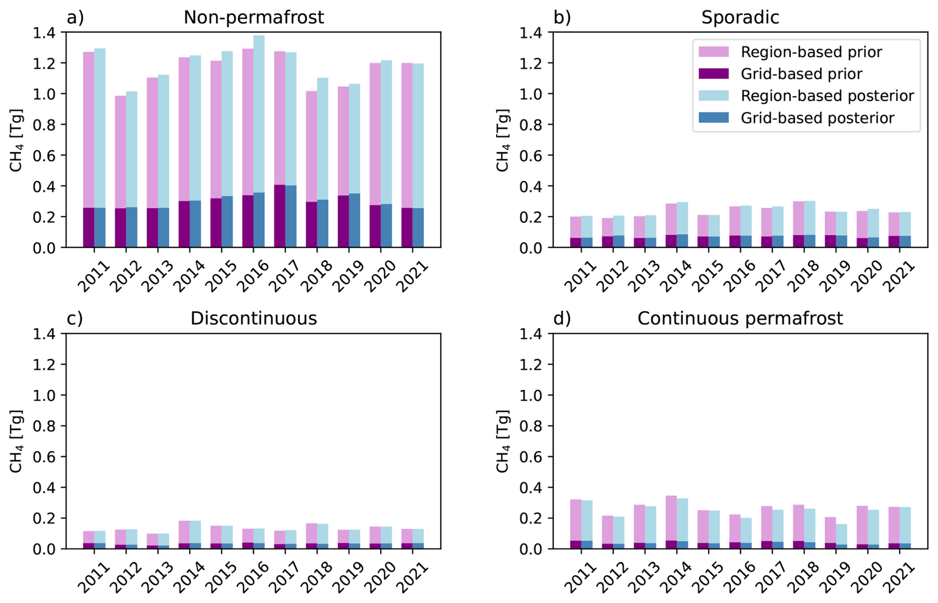
Figure 6 Total prior and posterior emissions in the four permafrost zones: (a) non-permafrost, (b) sporadic, (c) discontinuous and (d) continuous permafrost. The prior emissions are colored in purple and the posterior emissions in blue. The darker color represents the grid-based melt period emissions and lighter colors the region-based emissions.

To study which variables were linked to melt period methane emissions, the relationship between the length of the melt period and the posterior methane emissions was studied (Fig. 7). With both methods, the correlation between the length of the melt period and the total melt period emissions was positive in all the permafrost zones (Fig. 7a and c), indicating higher emissions during longer seasons. This relationship was most pronounced in the non-permafrost zone. The correlations were statistically significant in all zones for both methods (p<0.01).

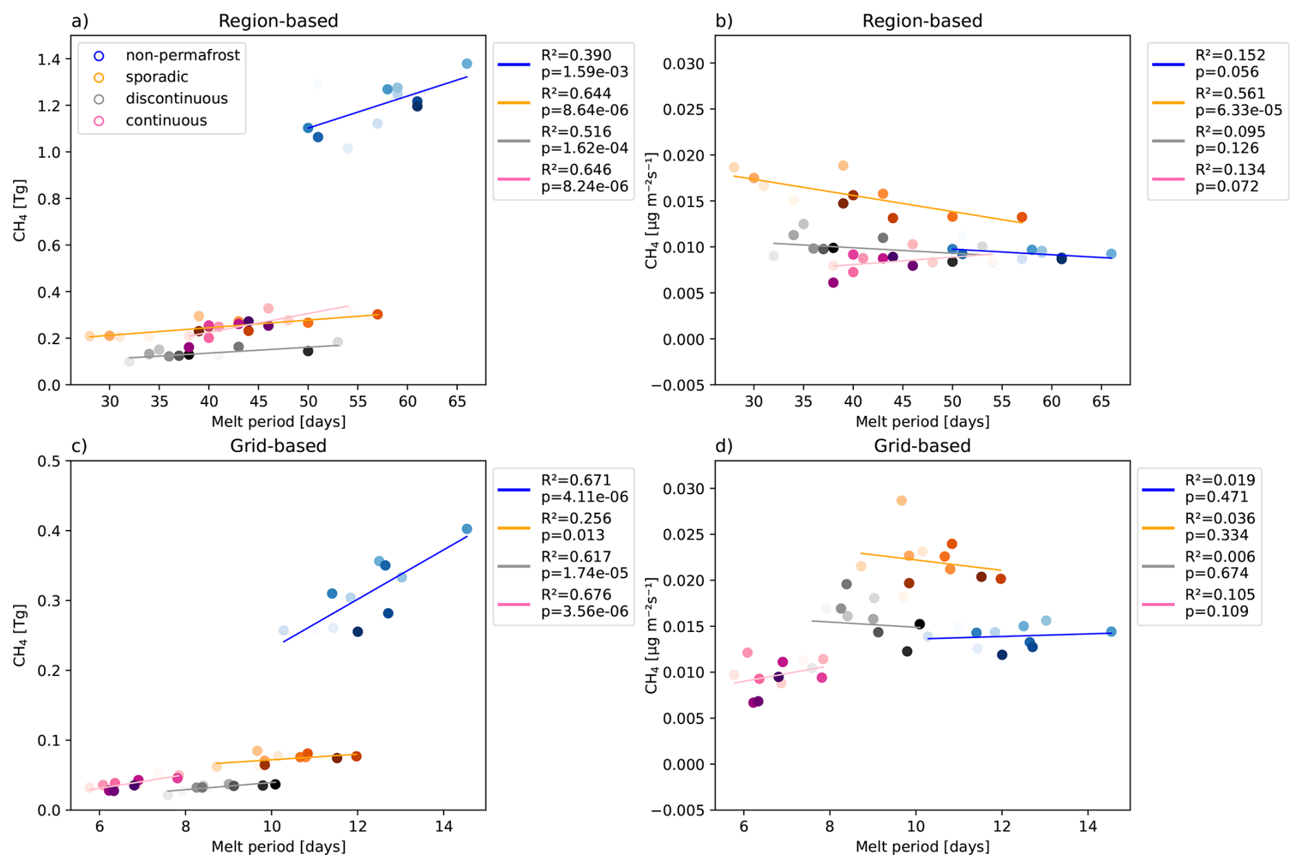
Figure 7 Panels (a) and (b) depict the region-based relationship between the total emissions (a) or the emission rate (b) and the length of the season. Panels (c) and (d) depict the grid-based relationship between the total emissions (c) or the mean emission rate (d) and the mean length of the melt period. Notice the different value range on the y axis in (a) and (c). The scatter plot color gradient represents the different years with 2011 being the lightest color and 2021 being the darkest. R² and p in the legends are the coefficient of determination and p-values of the slopes from linear regression fit, indicating statistical significance of the coefficient of determination.

Additionally, the posterior emission rate, as the units of $\mathrm{\mu }\mathrm{g}{\mathrm{CH}}_{\mathrm{4}}{\mathrm{m}}^{-\mathrm{2}}{\mathrm{s}}^{-\mathrm{1}}$, was calculated for the different zones (see Sect. 2.5.2). The correlation between the rate of emissions and the length of the melt period was not as clear as between the total melt period emissions and length, especially with the grid-based approach (p>0.05 in all zones) (Fig. 7d). There was a small negative correlation in the sporadic and discontinuous zones and positive ones in the other two zones. With the region-based approach, there was a stronger negative correlation in the sporadic zone between emission rate and length of the season (p<0.01) (Fig. 7b). In other zones, the correlation between emission rate and length was insignificant (p>0.05). The negative correlation in the sporadic zone could exist because of the negative correlation between the length and temperature of the melt period, and therefore the temperature would correlate positively with the emission rate. This relationship was studied in the grid-based Fig. A5, where grid cells with a negative emission rate were masked out, but no correlation was found in any of the zones. The region-based relationship between the variables was very similar. This indicates that the total emissions grew when the season was longer but there was no clear indication that the emission rate would be stronger or weaker when the season is longer.

Average posterior grid-based emissions in the Hudson Bay lowlands were 0.03±0.01 Tg and in the Western Siberian lowlands they were 0.11±0.04 Tg (Table A5). The corresponding region-based emissions in the Hudson Bay lowlands were 0.10±0.03 Tg and 0.47±0.14 Tg in the Western Siberian lowlands. An analysis of permafrost zone contributions in the Hudson Bay Lowlands and the Western Siberian Lowlands shows that, in most years, grid-based emissions were dominated by the non-permafrost zone. In 2012 and 2016 in the Hudson Bay lowlands, most emissions were from the sporadic zone, instead. With the region-based approach, most emissions were from the non-permafrost zone every year in both Hudson Bay lowlands and Western Siberian lowlands. The non-permafrost zone was the largest permafrost zone in both regions.

The years with the highest emissions in the entire northern latitude region were 2014 with the region-based approach, and 2017 with the grid-based approach (Tables A3 and A4). Maps of some of the highest emitting melt periods in the Hudson Bay lowlands and Western Siberian lowlands are shown in Figs. 8 and A6. Some of the grid cells with the highest emissions were located within these two lowland regions. However, the years with highest emissions in the Hudson Bay lowlands and Western Siberian lowlands differed from the years with highest emissions of the whole northern latitude regions. On the other hand, the years with the highest emissions in the Hudson Bay lowlands and Western Siberian lowlands matched between the two methods. The highest grid-based emissions in the Hudson Bay lowlands were found in 2012 and 2020, and region-based in 2012 and 2014. In the Western Siberian lowlands, the highest emissions were in 2014 and 2015 with both approaches. The highest emissions of the Western Siberian lowlands align better with the overall highest emitting years, likely due to the larger area of the Western Siberian lowlands to the Hudson Bay lowlands. However, there is no major difference in the emissions between the years in both regions. The average grid-based melt period length varied between the permafrost zones during the years with the most emissions in the Hudson Bay lowlands and the Western Siberian lowlands. During those years, at least one of the four zones in each lowland experienced a longer-than-average season. In the Hudson Bay lowlands during 2012 and 2020, the melt period was usually longer in a region where the mean temperature of the melt period was also colder than average. Same was seen in the Western Siberian lowlands in 2014.

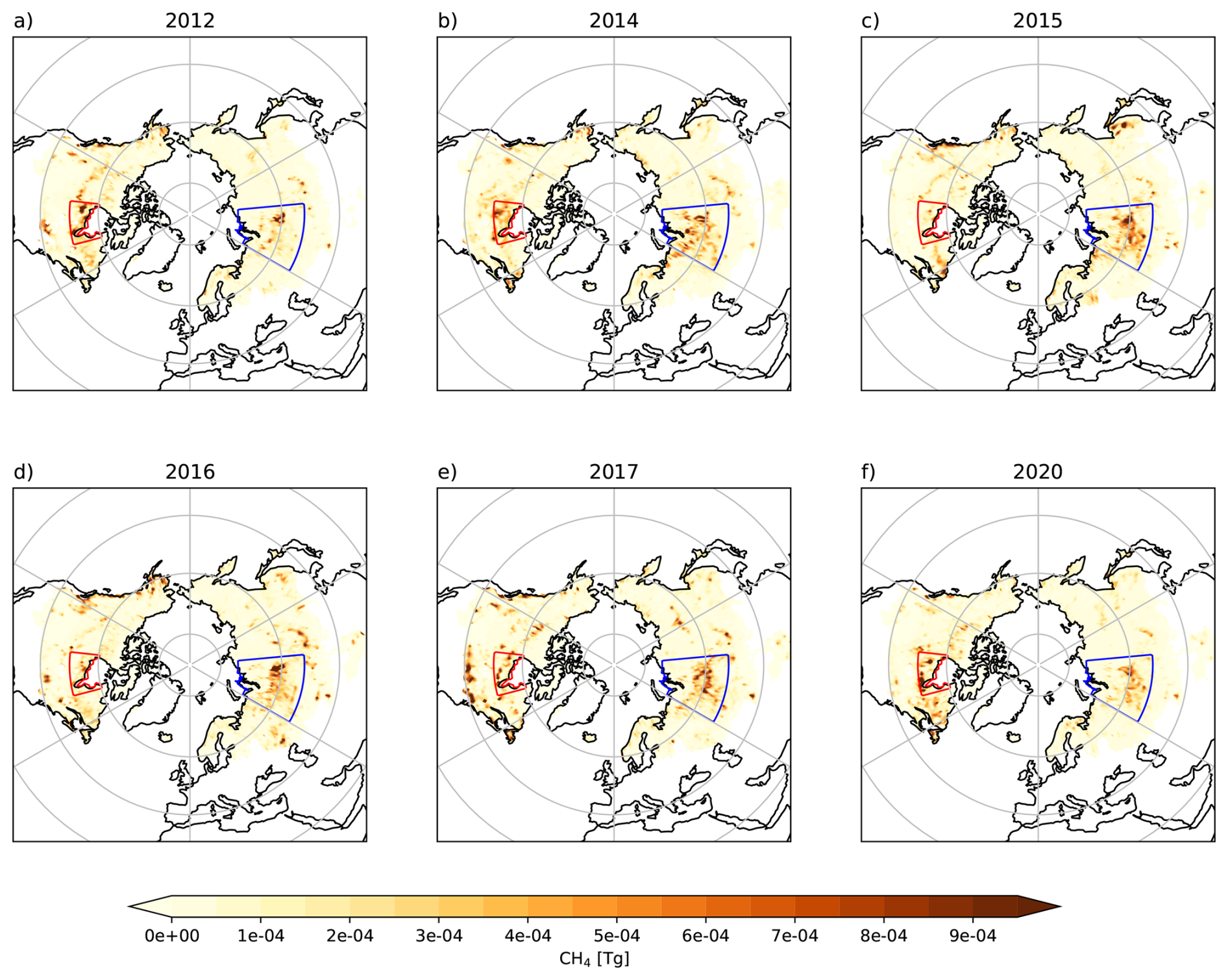
Figure 8 Grid-based emission maps of the melt period in the years that had some of the highest emissions in the Hudson Bay lowlands and Western Siberian lowlands. Hudson Bay lowlands have been outlined with red borders, and Western Siberian lowlands with blue borders.

The region-based melt period was not longer than the average in any of the zones in 2012, but in 2014, it was longer than the average in all the zones, except in the sporadic zone. In 2015, it was only longer than average in the non-permafrost zone. However, the region-based melt period was defined from the whole permafrost zone instead of only the area within Hudson Bay lowlands and Western Siberian lowlands, which might explain why the melt period was not exceptionally long during the years with highest emissions in these two regions. Both regions were also mostly covered by the non-permafrost zone, which explains why the emissions were generally larger when the melt period was longer in the non-permafrost zone.

Comparison to prior emissions

The total prior emissions during the melt period were 1.81±0.29 Tg with the region based approach and 0.447±0.11 Tg with the grid-based approach. This means that the inversion increased the total melt period emissions from the prior to the posterior. In the permafrost zones the inversion increased emissions from the prior in areas with less permafrost (Fig. 6a) and decreased in areas with more permafrost (Fig. 6d). This was more evident with the region-based approach and was seen the most distinctly in the non-permafrost and continuous permafrost zones. In the non-permafrost zone the posterior was almost always larger than the prior with both methods, despite already having the highest emissions. In the continuous permafrost zone the posterior emissions were always smaller than the prior emissions with both methods.

To see where the differences between prior and posterior emissions were most noticeable, we plotted a map of the total difference of the grid-based emissions during the melt period (Fig. A7) including the same years as in Fig. 8 and an average of all the years. The region-based figure was very similar to the grid-based, thereby only the grid-based figure is shown in the Appendix. Grid cells with no prior emissions during the melt period were masked out in the figure, though there were only a few. During these years, we can see spatial variation throughout the years. The most notable differences appear in the Western Siberian Lowlands and the Hudson Bay Lowlands region. The average region-based biospheric prior CH₄ emissions during the melt period in the Western Siberian lowlands were 0.45±0.11 Tg and in the Hudson Bay lowlands they were 0.09±0.026 Tg. The corresponding grid-based emissions in the Western Siberian lowlands were 0.11±0.03 Tg and in the Hudson Bay lowlands 0.03±0.01 Tg. The change from the prior to posterior is percentage wise larger in the Hudson Bay lowlands and Western Siberian lowlands than it is in the total northern high latitude region used in our study. In the total northern high latitude region, the posterior is about 1 % larger than the prior with both methods. In the Hudson Bay lowlands the posterior is about 6 % larger than the prior with both methods and in the Western Siberian lowlands it is about 3 % (grid-based) to 4 % (region-based) larger. In the four permafrost zones, the posterior emissions were 0.4 % (discontinuous permafrost) to 3 % larger (non-permafrost) or 6 % smaller (continuous permafrost) than the prior on average with the region-based approach. With the grid-based approach the posterior emissions were about 2 % larger (non-permafrost and sporadic zones) or 2 % (discontinuous) to 8.6 % (continuous permafrost) smaller than the prior on average.

We further examined the relationship between the difference in posterior and prior emissions and the length of the melt period (Fig. A8). Using the region-based approach, a significant positive correlation was found in the continuous permafrost zone between the difference in emission rate and melt-period length (p<0.05; Fig. A8b). In contrast, the grid-based approach revealed a negative correlation in the sporadic permafrost zone between melt-period length and both the emission difference (p<0.05) and the emission rate difference (p<0.01). Although differences between posterior and prior emissions were also observed in the other zones, no statistically significant correlations were detected between posterior-prior emission differences (or emission rate differences) and melt-period length. Overall, these results suggest that the inversion only marginally altered the relationship between emissions and melt-period duration.

4 Discussion

4.1 The melt period

4.1.1 Definition of the melt period and the SMOS F/T algorithm

The melt period occurring during springtime was defined for the northern high latitude wetlands for the first time based on the SMOS F/T data. As the SMOS F/T algorithm cannot distinguish between thawed soil and wet snow, it likely extended the season beyond the duration of true soil thawing. E.g. Tenkanen et al. (2021) found that the SMOS F/T data showed later soil freezing but earlier soil thawing than a process-based ecosystem model. However, it is justified to define the melt period to start from the melting of the snow (see Sect. 2.5.1). In addition, including either snow depth data from in-situ measurements or fractional snow cover data from satellites could have helped our algorithm to detect the starting of the soil thawing.

The amount of SMOS F/T pixels in a 1°×1° grid cell made the definition of melt period spatially inconsistent. The number of pixels decreased towards the north, requiring a higher fraction of thawed soil in northern grid cells before the melt period began. However, with our definition, the absolute area, which had to be thawed before the season could start, was similar across the study area, though it also meant that the estimated thawing state of the soil was more uncertain if there were missing SMOS F/T datapoints. The difference in the amount of pixels in a grid cell might have introduced systematic biases, causing longer melt periods in south and shorter in north.

With both methods, the melt period generally started the earliest in the southern regions. However, there were some mountainous regions in the south, for example, the mountains in Mongolia, and the Rocky Mountains in the western coast of North America (Fig. 3), where the season started and ended later, causing long melt periods. This is likely due to higher altitude and lower temperatures. The SMOS F/T data is not as reliable in the mountainous regions as it is elsewhere, mainly because there is less soil substance, especially at higher elevations. Since the SMOS satellite measures the soil freezing through the permittivity difference between ice and water, it does not measure the soil freezing correctly in areas with less absorbent soil. Thus, the melting of snow or ice on solid rock does not significantly affect what is measured. A sufficient difference between thawed and frozen states requires soil that has absorbed water. Additionally, the topography affects the remote sensing measurements: the measurement angle varies a lot in the mountains, which means that with different measurement angles, the measured thawing state of the soil also changes.

4.1.2 Region-based and grid-based melt period

The region-based melt period was on average about 4 times as long as the grid-based melt period. The region-based approach does not represent the local melt period accurately because of the substantial area of the permafrost zones and the difference between the start and end days inside one zone was large. In other words, the melt period in the southern grid cells might have already ended, while soil was still frozen in northern parts of the zone. However, with this method, the thawing fraction varied less during the melt period, and the beginning and end of the melt period were more consistent, making it easier to compare the different permafrost zones' melt periods and methane emissions with each other on a larger climatological scale.

The grid-based melt period was on average almost twice as long in the southernmost zone: non-permafrost (12 d) compared to the northernmost permafrost zone: continuous permafrost (7 d). This suggests that the season was shorter when there was more permafrost and the further north the region was, except for the mountainous permafrost regions in the south (Fig. 3). In a small area, the soil melts almost simultaneously leading to a shorter melt period. Additionally, because the grid-based period could not begin before the minimum thaw fraction was exceeded for the final time in spring, some grid cells may have experienced fluctuations in thaw fraction prior to this date. This variability could therefore have been included within the defined melt period. However, with this method the melt period was separated from the autumn freezing season if it continued past the turn of the year.

Each of the four permafrost zones consisted of areas in the North American and the Eurasian continents. Especially the region-based melt period could have been more precise if it was defined separately for the two continents due to their different year-to-year variability of climates.

4.1.3 Timing and length of the melt period

Different methods used to study the timing of snowmelt and spring thawing season have produced varying results. According to the definitions of the Finnish Meteorological Institute (FMI) based on temperature data, spring starts approximately in the middle of March in southern Finland and in April in northern Finland (Ilmatieteen laitos, 2025) and lasts for two to four weeks during which snow melts and the growing season starts. Our estimated melt periods in Finland, which is located mostly in the non-permafrost area, coincide with this: on average, the melt period started in March–April using both the grid-based and the region-based methods.

According to regional studies in northern Alaska, underlain by continuous permafrost, the spring thawing season in the tundra region was approximately 20 d long (Zona et al., 2016; Bao et al., 2020), which is shorter than the region-based melt period defined here (45 d on average, Table A2) and longer than the average grid-based melt period (10 d). With our grid-based method, the average length of the melt period during our study period in the grid cells closest to the coordinates of the measurement stations used by Zona et al. (2016) and Bao et al. (2020) varied between 4–19 d. Overall, in many grid cells in the whole northern high latitude domain, the length of the melt period was ∼20 d. Both Zona et al. (2016) and Bao et al. (2020) used soil temperature data to define the thawing of the soil. We did not use in-situ soil temperature data in this study as in-situ measurements of frozen soil are rare, and thus not suitable for our larger region study. Other option would have been to use reanalysis soil temperature data such as ERA5, which has shown higher skills than other products and a significant improvement over its predecessor (Li et al., 2020). However, it is not well-suited for permafrost research (Cao et al., 2020). Thus, SMOS F/T data is a good proxy for the soil thawing.

The SMOS F/T data starting the melt period already from the melting of the snow instead of the soil is likely the reason for the longer region-based melt period. According to our prior LPX–Bern DYPTOP v1.4 (Fig. A9), the soil temperature rose to 0 °C during the region-based melt period on all permafrost zones. This means that the SMOS F/T melt period started earlier than the process-based ecosystem model melt period. However, the prior had a monthly temporal resolution compared to the daily resolution of the SMOS F/T data, and so the soil temperature rising above 0 °C in the middle of the melt period is a good indicator for the correct timing of our melt period.

According to the prior emissions used in this study (LPX–Bern DYPTOP v1.4), peat emissions were relatively high during the melt period compared to emissions from inundation for all other permafrost zones but continuous permafrost (Fig. A9). However, even in the continuous permafrost zone, the peat emissions are higher than those from inundation in April, and are rising during the melt period. At the beginning of spring, extensive snow melt inundation causes a large part of methane emissions, and after the end of the melt period, the methane emissions are dominated by peat emissions. Even though methane emissions from peat dominated over emissions caused by inundation for a large part of the year, there were evident peaks in inundation emissions in every permafrost zone during and/or right after the melt period. This indicates that the melt period timing we defined is reasonable.

4.2 Methane emissions during the melt period

The way we defined the melt periods affected the estimated melt period methane emissions. The emissions were optimized weekly, which were interpolated linearly to daily values from one optimized weekly value to the next weekly value before the calculation of the melt period emissions. This introduced a new source of uncertainty and affected the estimated melt period methane emissions, especially when using the grid-based approach, as the length of the grid-based season was much shorter and often less than a week (between 51 % of the grid-cells in the non-permafrost zone and 70 % in the continuous permafrost zone).

In the Hudson Bay lowlands and Western Siberian lowlands, as wells as in the four permafrost zones, the methane emissions were distributed unevenly (Fig. 8). This may be explained by the distribution of wetlands within the lowlands, as wetlands generally exhibit higher methane emissions than other land-cover types, such as forests, which might even be a sink of methane. The years with highest emissions were distributed evenly across the study period (Fig. 8), indicating that there is no clear evidence of increasing melt period emissions.

4.2.1 Methane bursts during the melt period

Multiple previous studies have shown higher emission rates to our results with many of them showing large bursts of CH₄ from wetlands during the spring thawing season (Jin et al., 1999; Tokida et al., 2007; Song et al., 2012; Tagesson et al., 2012; Mastepanov et al., 2013; Zona et al., 2016; Raz-Yaseef et al., 2017; Bao et al., 2020). These events typically last for a short time, from few hours to a few days (Song et al., 2012). Such emission bursts could have caused large emissions even during a shorter melt period, causing the relationship between the length and the emissions of the melt period to be non-linear. However, we found a positive correlation between the total melt period methane emissions and length, which was observed with both the grid-based and the region-based methods in permafrost zones and Western Siberian and Hudson Bay lowlands. This indicates that the bursts were not large enough to be detected with our model resolution (1°×1°) and weekly temporal optimization of the fluxes. The emission rates were also estimated from the whole area of the 1°×1° grid cell instead of the wetland area, which made the emission rates smaller compared to the local studies. Another reason for the positive correlation between the values could be that in our study, we focused on emissions within larger permafrost zones. In individual grid cells, some emission peaks could have been detected but that was not explicitly studied here. Above mentioned studies reporting large CH₄ bursts during the spring thaw used field measurements to define the emission rate which have sensitivity for smaller areas compared to our inverse model. Emission rates defined from the eddy covariance measurement measure the local methane bursts rather than the average rates from a larger permafrost zone.

Using a process-based model Castro-Morales et al. (2018) showed an emission rate closer to what we found in this study. The atmospheric inverse model used here used atmospheric CH₄ measurements to inform and “re-evaluate” the process-based estimates. In most years, our inversion showed an increase from the prior emission estimates which were based on the process model LPX-Bern DYPTOP. This means that there might have been short-lived emission bursts during the melt period, which the process model was not able to produce due to the poor spatial and temporal resolution or missing processes, or that the process model emission estimates were overall too low during this period.

With our inverse model, the grid-based emission rates were higher in some grid cells (Fig. A5), and on average, the grid-based emission rates were higher than the region-based (Fig. 7). The grid-based melt period likely represents local emission bursts during soil thawing better than the region-based approach. Within a single permafrost region, fluxes vary widely because the area does not consist entirely of permafrost or wetlands. This lowers the CH₄ emission rate. The local measurement studies might be more comparable to the melt period emissions in the Hudson Bay lowlands and Western Siberian lowlands in grid cells, where the total area of the cell is mostly wetland. However, the focus of this study was to estimate the total melt period emissions rather than occasional hotspots.

4.2.2 Magnitude of the melt period methane emissions

According to Saunois et al. (2025), the annual global methane emissions estimated from atmospheric inversions were 575 [553–586] Tg CH₄ yr⁻¹, in 2010–2019. Of these emissions, 165 [145–214] Tg CH₄ yr⁻¹ were from wetlands. The average global biospheric emissions using the CTE-CH₄ data from this study for the years 2011–2021 were 124 Tg CH₄ yr⁻¹, including also soil sink (LPX-Bern DYPTOP prior soil sink 33 Tg CH₄ yr⁻¹). In the northern high latitudes (defined in the chapter 2.3), the average annual methane emission were 23 Tg CH₄ yr⁻¹. The region-based melt period posterior emissions were 1.83 Tg (8.1 % of the annual northern high latitude emissions) and grid-based were 0.45 Tg (2 % of the annual northern high latitude emissions), only a small portion of the annual total global emissions. The length of the melt period with the grid-based method was 3 %, and with the region-based method 12 %, of the total length of a year.

Methane emissions during other seasons and the high northern latitudes have been studied previously. According to Tenkanen et al. (2021), the winter cold season (November to April) emissions were 3.3 Tg in the northern high latitudes (above 50° N), which included partly emissions from both the autumn freezing and spring thaw seasons. The autumn freezing season methane emissions from the same model with a different setup were 1 Tg (Tenkanen, 2019). Erkkilä et al. (2023) estimated the autumn freezing, winter cold season and summer thaw season emissions in the northern high latitudes with the same inverse model but a different setup to ours. They found emissions to be 1.2 Tg in winter, 0.73 Tg in the freezing period, and 16.2 Tg in the thaw (summer) period. In both studies, winter and freezing season emissions were smaller than our region-based melt period emissions but larger than the grid-based emissions.

According to a study which used upscaled flux measurements, the methane emissions during the melting of the soil in wetlands in a northern high latitude permafrost region were 0.5–0.97 Tg in 2011 (Song et al., 2012). In a study by Ito et al. (2023), the spring season (March–May) methane emissions were calculated with multiple process-based ecosystem models for the northern wetlands (>45°), and their mean value was $\mathrm{0.80}\pm \mathrm{1.89}\mathrm{Tg}{\mathrm{CH}}_{\mathrm{4}}{\mathrm{yr}}^{-\mathrm{1}}$ (3.07 %±9.61 % of the annual emissions), where the error is the variation between the maximum and minimum model result. These estimates are closer to the grid-based emissions estimated in this study.

Defined from the inverse model used in this study, the mean annual emissions in the Hudson Bay lowlands and Western Siberian lowlands were the size of 2.9 and 5.0 Tg, respectively. This is close to the values defined in other studies (Thompson et al., 2017; Peltola et al., 2019; Tenkanen et al., 2021). The average region-based melt period emission in the Hudson Bay lowlands and the Western Siberian lowlands were the size of 0.1 and 0.47 Tg, respectively. The grid-based emission were smaller with the magnitude of 0.03 and 0.11 Tg, respectively. This means that together they produced approximately 31 % of the total melt period emissions from the northern high latitude wetlands with both methods. This is a significant part of the total melt period emissions when their areas only represent a portion of the total study region (Hudson Bay lowlands is 2.5 % and Western Siberian lowlands is 9.6 % of the total study region land area). The region-based melt period emissions were 7 % and grid-based emissions were 1.7 % of the annual emissions from the Hudson Bay lowlands and the Western Siberian lowlands. The increase in emissions from prior to posterior estimates was also more pronounced in these two regions than across the northern high-latitude domain as a whole. This may be attributed to the greater extent of continuous wetlands in these regions and/or the higher density of the observational network (Fig. A1), which likely influenced the prior estimates. Additionally, there are large areas in the high northern latitudes, where the difference between the posterior and prior emissions was close to zero during the melt period (Fig. A7). In grid cells where prior emissions were zero, posterior emissions during the melt period were also zero. This likely contributed to the minimal differences observed between prior and posterior estimates in those areas. However, the emissions in the Western Siberian lowlands could have been overestimated, because the NIES observation sites, which we did not adjust before using the measurements in the inversion, had a different calibration scale (3.0 to 5.5 ppb higher) than WMO CH4 X2004A scale as in the ObsPack (Sasakawa et al., 2025). The NIES observations are now included in the newer version of ObsPack, with scale corrected. A higher density of observations in the northern high latitudes could have improved our inverse method estimates.

5 Summary and conclusion

The melt period was defined for the northern high latitude wetlands with the SMOS F/T soil thawing data separately for four permafrost zones: seasonally frozen non-permafrost, sporadic, discontinuous and continuous permafrost. The melt period was defined separately with a region-based and a grid-based approach. The region-based method is comparable to studies with monthly emission estimates, as it focuses more on the climatological differences between large regions, while the grid-based method is more comparable to local studies. The region-based period started and ended the earliest in the southernmost permafrost zone and latest in the northernmost zone. With the grid-based approach, there was more variation in the start and end days of the season in the north-south direction mostly because of the mountainous regions. The region-based melt period lengths varied more from year to year than the grid-based seasons, with he non-permafrost zone having the longest season on average with both methods. The average grid-based melt period was shortest in the continuous permafrost zone and the region-based was shortest in the sporadic and discontinuous zones. We found that the length of the melt period was dependent on the average 2 m temperature of the melt period, with a longer season having a lower mean temperature. This could have been caused by the early onset of melting, followed by variation between temperatures, making the mean temperature of longer seasons lower. We found the SMOS F/T data to be useful in estimating the melt period, and for example, using it to inform process-based models to account for soil freeze/thaw state could lead to better constrained methane emission estimates.

In the four permafrost zones, the melt period methane emissions were the largest in the non-permafrost zone and the smallest in the discontinuous zone with both methods. The total region-based melt period emissions for the four zones were 1.83±0.27 Tg CH₄ per season and grid-based emissions were 0.45±0.10 Tg CH₄ per season. These emissions represented 8.1 % and 2 % of the total annual northern high latitude emissions according to our inverse model results (23 Tg). We found that the total melt period emissions depended on the length of the melt period, with more methane emitted during longer seasons.

We additionally studied the emissions in the Hudson Bay lowlands and Western Siberian lowlands, as they are the largest wetlands in the northern high latitudes. Their melt period methane emissions were a significant portion of the total melt period emissions (31 % with both methods and both lowlands combined) but only a small part of the total annual northern high latitude emissions (2.5 % with the region-based approach and 0.6 % with the grid-based approach). The Western Siberian lowlands had higher emissions than the Hudson Bay lowlands with both methods, likely due to its' larger size, even though it had a slightly shorter and colder grid-based melt period on average than the Hudson Bay lowlands.

The total melt period emissions in the northern high latitudes were only a small portion of the total annual emissions. However, future climate change and associated permafrost thawing could amplify melt period emissions, resulting in elevated CH₄ bursts. Our results showed that the melt period was the longest with highest emissions in the non-permafrost region where the average temperature is higher throughout the year. On the other hand, our results showed that when the mean temperature was higher on average during the melt period, the period was shorter and had smaller total emissions.. Increasing temperatures could instead lead to shorter melt periods and consequently lower melt period methane emissions. Subsequently, a longer summer thaw season could lead to higher annual emissions. However, it is still unclear how climate change feedback loops will affect emissions and shoulder season lengths in the northern high latitudes, as permafrost thawing and soil drying could lead to higher CO₂ emissions instead. To get a better look at the melt period emissions, the results from several inversions could be compared to each other. In addition, going further to the level of individual wetlands and comparing their flux measurements during the melting could bring more clarity to true wetland emissions.

Appendix A

Table A1 List of surface observation sites used in inversions. Observation Uncertainty (Obs. Unc.) is used to define diagonal values in the observation covariance matrix. The data type is categorized into two measurements (discrete (D) and continuous (C)).

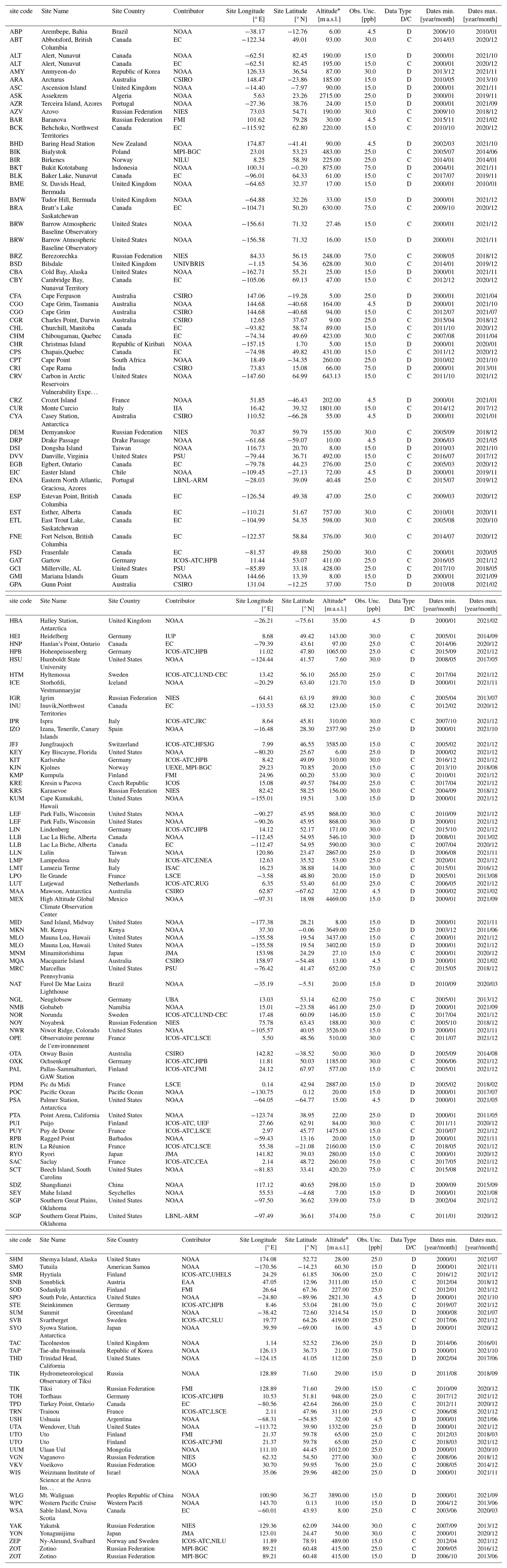
*Sampling heights from which atmospheric CH₄ is sampled in TM5. **Observations used in this study between 2010 and 2021.

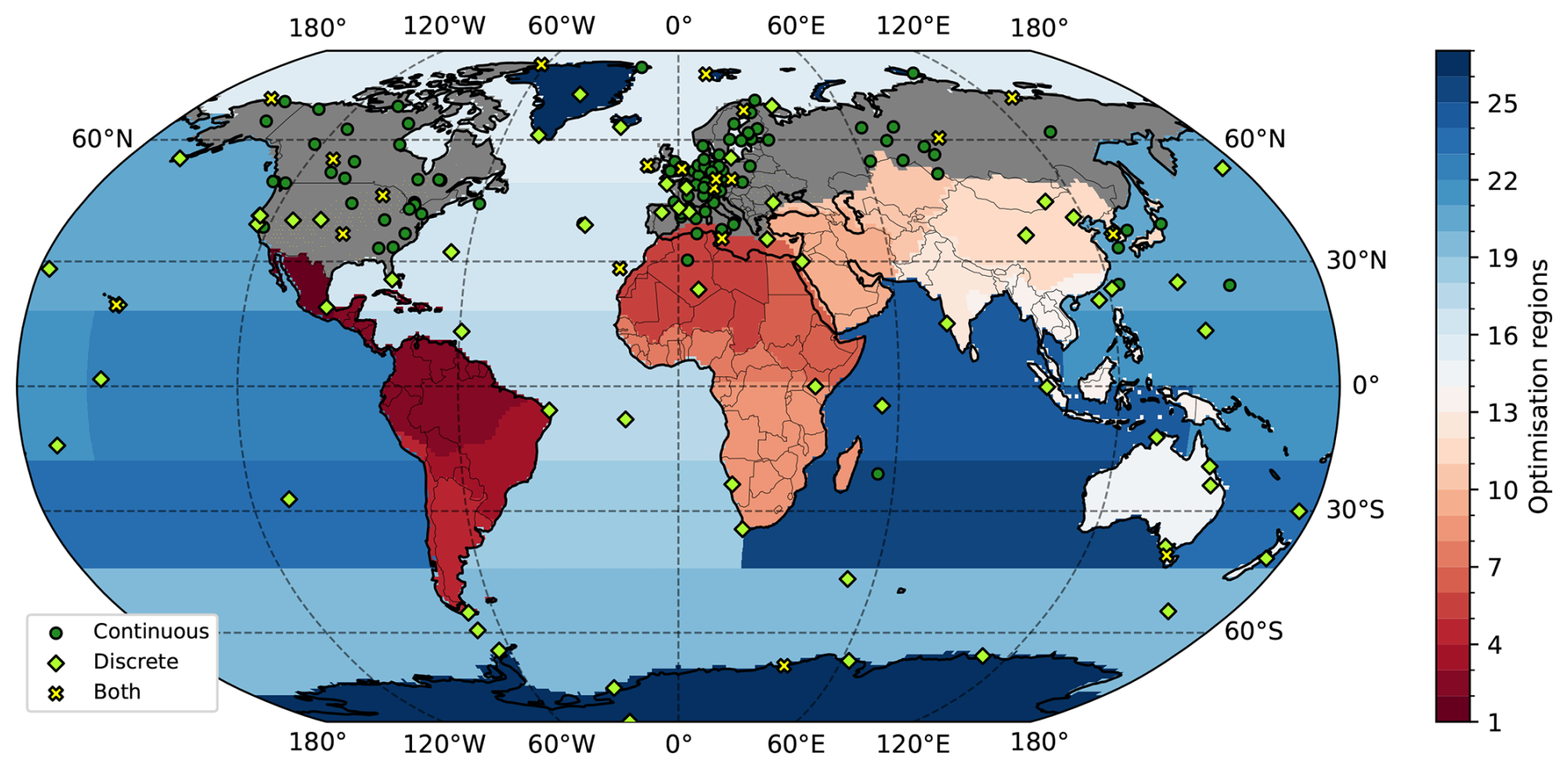
Figure A1 The locations of the atmospheric CH₄ measurement sites and the type of measurement used (continuous, discrete or both) in the inversions. The areas optimised regionally are shown with blues and reds, and the grey colour shows the area optimised at 1° latitude × 1° longitude resolution.

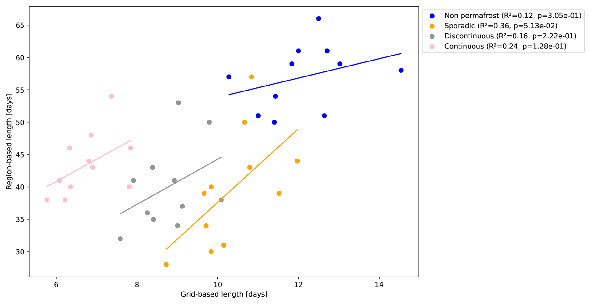
Figure A2 Relationship between grid-based and region-based melt periods in 2011–2021. R² and p in the legends are the coefficient of determination and p-values of the slopes from linear regression fit, indicating statistical significance of the coefficient of determination.

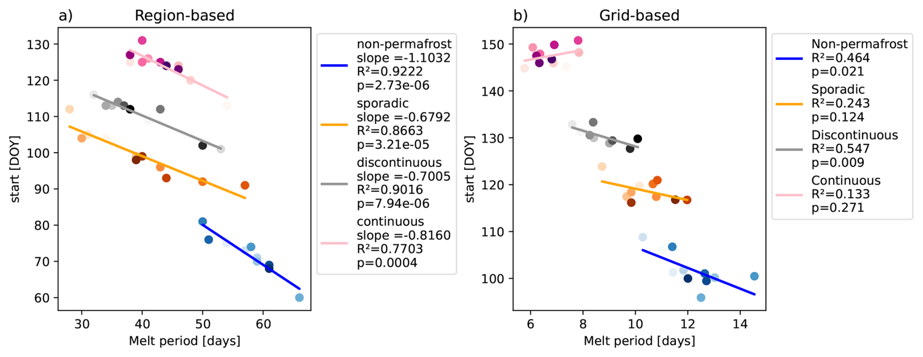
Figure A3 Relationship between region-based melt period and its' starting day (a) and grid-based melt period and its' average starting day (b) in 2011–2021. R² and p in the legends are the coefficient of determination and p-values of the slopes from linear regression fit, indicating statistical significance of the coefficient of determination.

Table A2 Region-based melt period start and end days, as well as the length of the melt period in days for the four permafrost zones: non-permafrost, sporadic, discontinuous and continuous permafrost defined for each zone. The start and end days are represented as a number of days from the beginning of the year, with number one being the first day of the year (day-of-year).

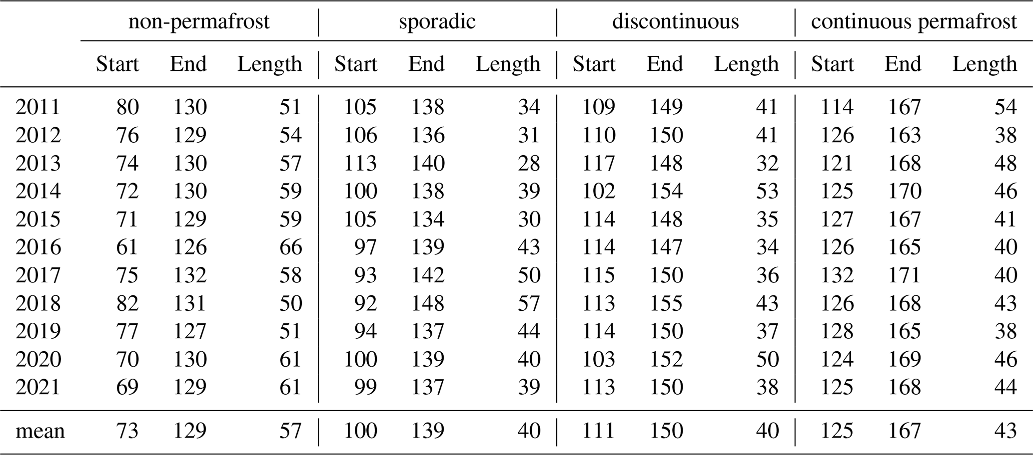
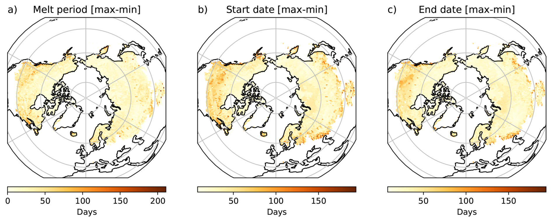
Figure A4 Grid-based difference between the maximum and minimum length (a), start day (b) and end day (c) of the melt period during the study period (2011–2021).

Table A3 Region-based posterior melt period methane emissions in the four permafrost zones; non-permafrost, sporadic, discontinuous, and continuous permafrost, as well as the total sum of the emissions.

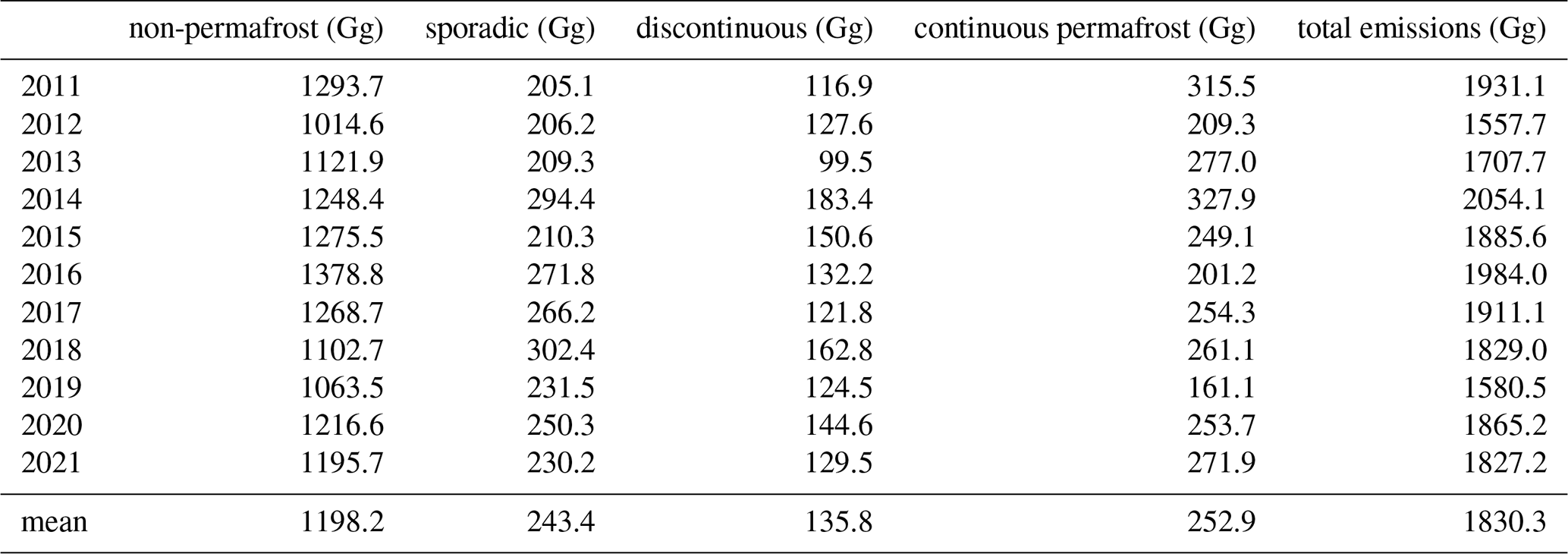
Table A4 Grid-based posterior melt period emissions in the four permafrost zones; non-permafrost, sporadic, discontinuous, and continuous permafrost, as well as the total sum of the emissions.

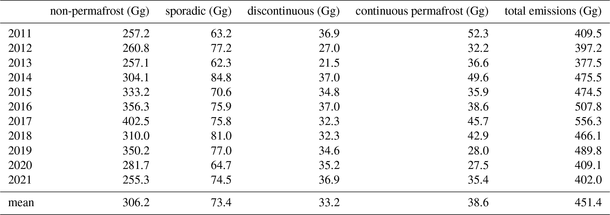
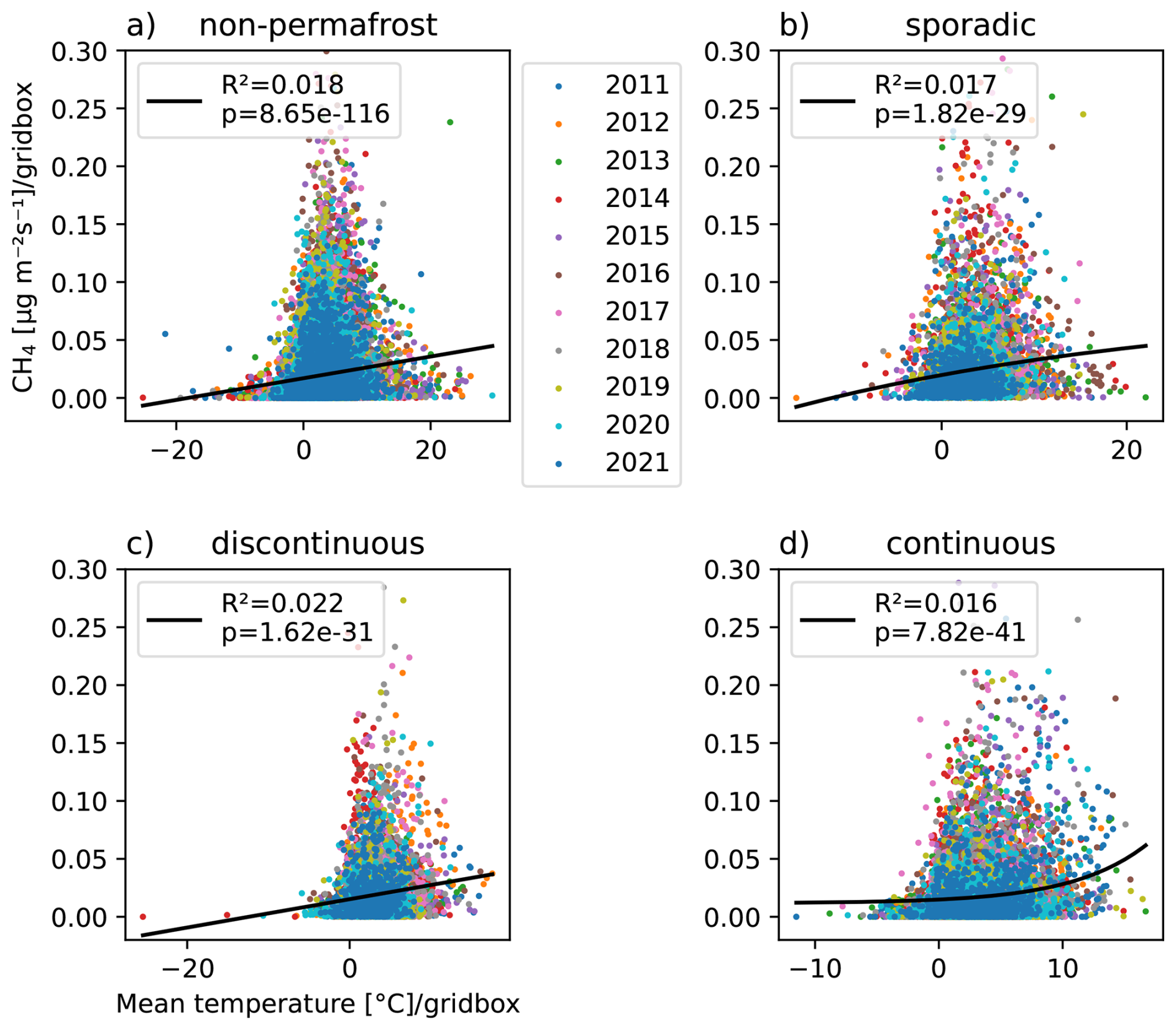
Figure A5 Grid-based posterior melt period methane emissions and the mean temperature in the four permafrost zones; (a) non-permafrost, (b) sporadic, (c) discontinuous, and (d) continuous permafrost. grid cells with negative emission rate were masked out. R² and p in the legends are the coefficient of determination and p-values of the slopes from linear regression fit, indicating statistical significance of the coefficient of determination.

Table A5 Melt period posterior methane emissions in the Hudson Bay lowlands and Western Siberian lowlands.

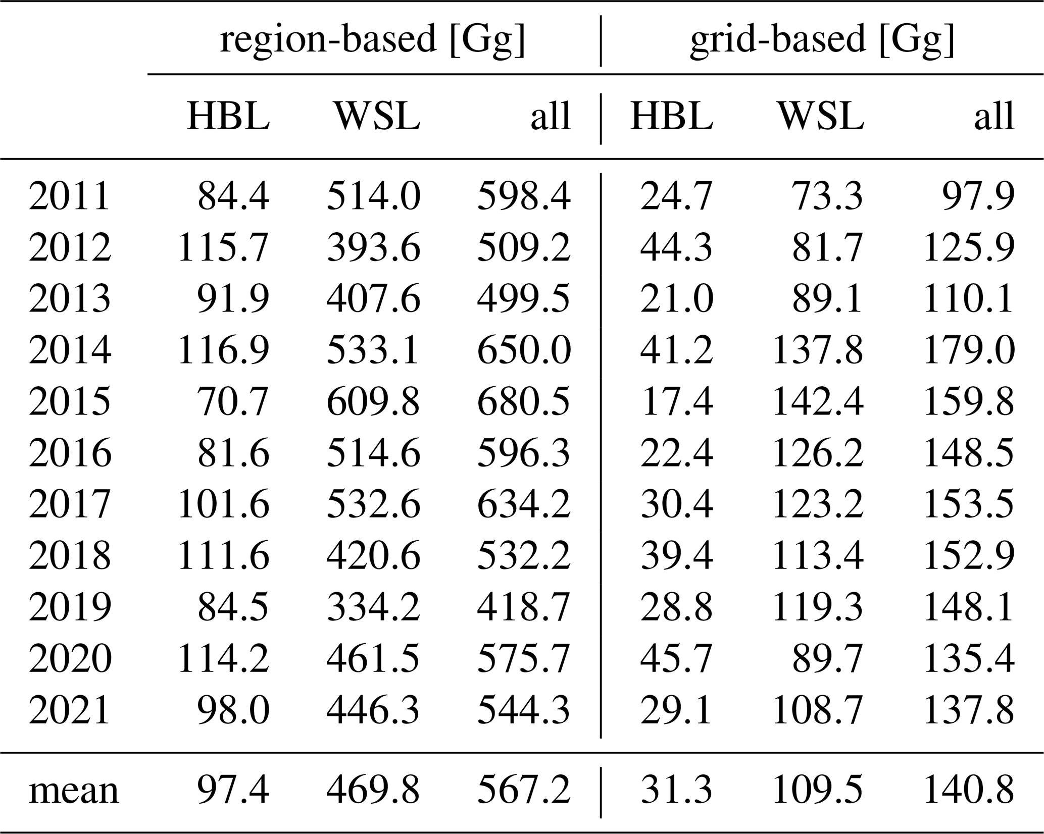
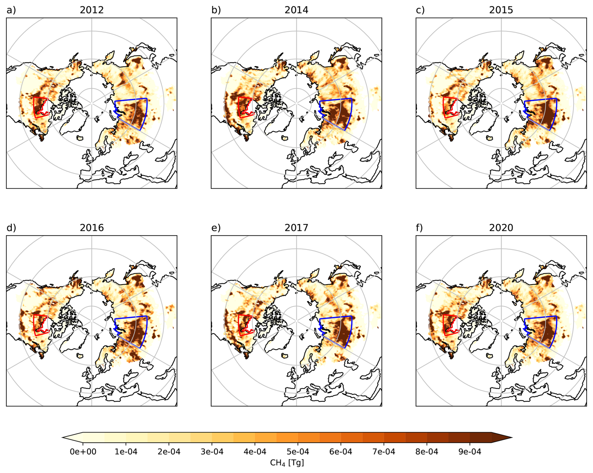
Figure A6 Region-based posterior emission maps of the melt period in the years that had some of the highest emissions in the Hudson Bay lowlands and Western Siberian lowlands. Hudson Bay lowlands have been outlined with red borders, and Western Siberian lowlands with blue borders.

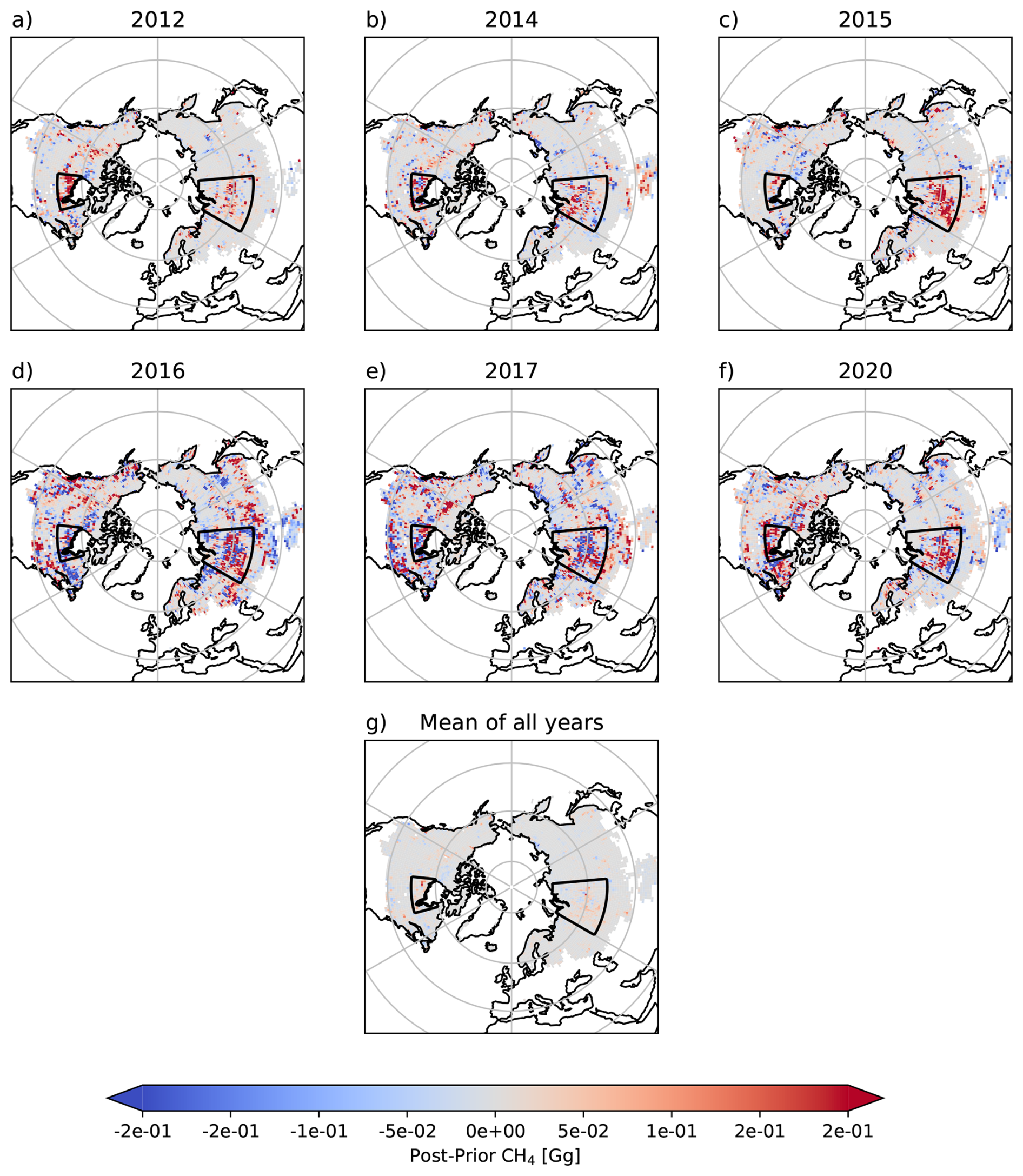
Figure A7 Difference between prior and posterior emissions of the melt period in the years that had some of the highest emissions in the Hudson Bay lowlands and Western Siberian lowlands (a–f) as well as the mean difference of all years of this study (g). Hudson Bay lowlands and Western Siberian lowlands have been outlined with black.

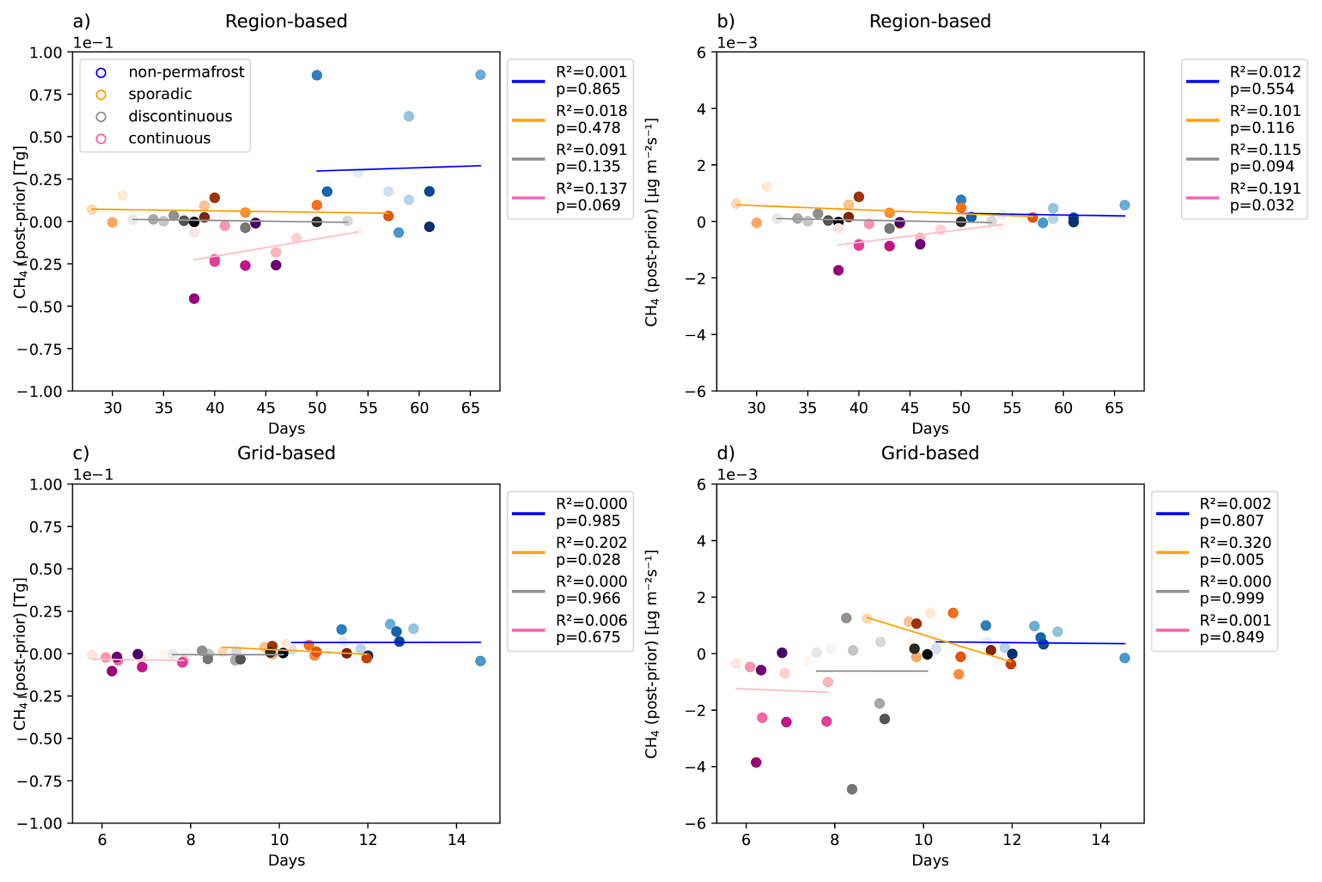
Figure A8 Panels (a) and (b) depict the region-based relationship between the difference of prior and posterior total emissions (a) or the emission rate (b) and the length of the season. Panels (c) and (d) depict the grid-based relationship between the difference of prior and posterior total emissions (c) or the mean emission rate (d) and the mean length of the melt period. The scatter plot color gradient represents the different years with 2011 being the lightest color and 2021 being the darkest. R² and p in the legends are the coefficient of determination and p-values of the slopes from linear regression fit, indicating statistical significance of the coefficient of determination.

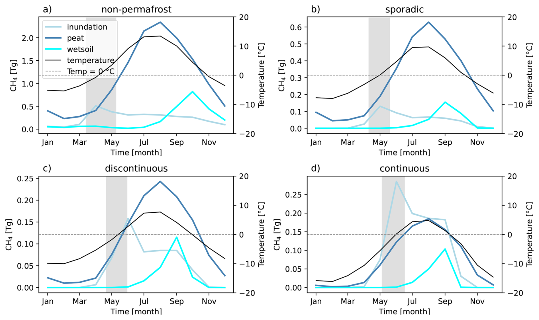
Figure A9 Average monthly emissions from peat, inundation and wetsoil for the years 2011–2019, from the prior LPX–Bern DYPTOP v1.4 emissions. Average temperature is indicated by a black line. The average region-based melt period is showed with gray shading.