Errors in satellite-based global horizontal irradiance retrievals due to three-dimensional cloud-radiation interactions

Observations of sunlight reaching the Earth's surface are crucial for a range of applications, including accurate monitoring and nowcasting of solar energy. Satellite retrieval algorithms for global horizontal irradiance (GHI) are generally one-dimensional (1D), assuming horizontally independent and homogeneous pixels, called the independent pixel approximation (IPA) and plane-parallel approximation (PPA), respectively. In reality, clouds scatter radiation in three dimensions, introducing retrieval errors which, without prior knowledge of three-dimensional (3D) cloud structures, remain unknown. This study assesses the PPA and IPA validity in GHI retrievals for two highly variable cumulus cloud fields at spatial resolutions ranging from 0.05 to 12.8 km at varying geometries and surface albedos. Using accurate 3D Monte Carlo radiative transfer (RT) simulations, synthetic top-of-atmosphere reflectances are generated, from which GHI is retrieved. GHI calculated directly from the input using 1D and 3D RT serves as a reference. We explain how horizontal photon transport causes GHI underestimations in clear-sky regions, while in cloud shadows GHI is overestimated. Furthermore, towards coarser spatial resolutions, the PPA introduces retrieval biases due to mixing of cloudy and clear-sky reflectances. In most simulations, domain-averaged biases are minimal at a resolution of 1 to 3 km. In terms of root mean square error, the largest disagreements are observed at the finest spatial scales, with IPA-related errors dominating for resolutions finer than about 2 to 6 km. The current generation of geostationary satellites already resolves these finer spatial scales. Therefore, this work emphasises the need to develop 3D RT parametrisations and corrections for GHI retrievals.

1 Introduction

Solar irradiance reaching the Earth's surface is an important quantity for studying the radiative balance and dynamic processes in the Earth's atmosphere (e.g. Liou, 2002; Visconti, 2016; Platzer and Stieglitz, 2024; Spiridonov et al., 2025). In the presence of clouds, solar radiation is scattered, which can lead to highly variable irradiance fields varying at scales down to seconds or metres (Mol et al., 2024). Retrievals of global horizontal irradiance (GHI) from geostationary satellites provide a unique data source for capturing larger-scale variability owing to their coverage of a vast geographic area in combination with a kilometre-scale spatial resolution and short revisit times.

GHI retrievals from geostationary satellites have a wide range of possible uses. Applications include climate monitoring (Ma and Pinker, 2012; Pfeifroth et al., 2024), validation of weather and climate models (Freidenreich and Ramaswamy, 2011; Alexandri et al., 2015; Chen et al., 2024) and assessment of agricultural yield and water availability through the derivation of estimates on the surface energy fluxes and evapotranspiration (Trigo et al., 2018; Barrios et al., 2024). Furthermore, the energy transition towards an energy mix with a high share of renewable energy sources makes GHI retrievals of special interest for real-time estimation and nowcasting of photovoltaic (PV) power generation (Hammer et al., 1999; Arbizu-Barrena et al., 2017; Cui et al., 2024).

The Flexible Combined Imager (FCI) onboard the third generation of Meteosat satellites (MTG; Holmlund et al., 2021) enables the retrieval of clouds and GHI down to 500 m scales over Europe and Africa. This is a sixfold increase in resolution compared to retrievals from FCI’s predecessor, the Spinning Enhanced Visible and Infra-Red Imager (SEVIRI) onboard the second generation of Meteosat satellites (MSG; Schmetz et al., 2002). Although one might expect that the increase in spatial resolution improves the GHI retrieval accuracy, the actual effect of this improved resolution is not yet clear.

A range of methods (e.g. Mueller et al., 2009; Huang et al., 2011; Greuell et al., 2013; Qu et al., 2017; Huang et al., 2019; Pfeifroth et al., 2024) exists to retrieve GHI from passive satellite imagery. Despite these different methods, they all rely on two general assumptions.

The first assumption is the plane-parallel approximation (PPA; Cahalan et al., 1994). The PPA assumes that all retrieved pixels are fully horizontally homogeneous. Any potential sub-pixel variability is unknown and not accounted for. Since the relation between reflectance, cloud properties, and GHI is highly nonlinear, neglecting the sub-pixel variability may introduce biases. By resolving clouds at finer resolutions, the validity of the PPA increases (Zinner and Mayer, 2006).

The second assumption is the independent pixel approximation (IPA). The IPA assumes that reflectances from each pixel are independent of those from neighbouring pixels (Cahalan et al., 1994). This means that the horizontal transport of photons is disregarded. At finer pixel sizes, horizontal photon transport becomes increasingly relevant, and thus the validity of the IPA decreases (Zinner and Mayer, 2006). By assuming pixels are independent, three-dimensional (3D) radiative effects such as cloud shadow displacement and irradiance enhancements, in which pixels receive direct radiation from the Sun as well as scattered radiation from clouds in the vicinity, are not represented.

In principle, the IPA error could be addressed by employing 3D radiative transfer (RT) methods (e.g. Marshak and Davis, 2005; Emde et al., 2010; Villefranque et al., 2019; Veerman et al., 2022; Trees et al., 2025). However, because of the high computational cost of resolving radiation in three dimensions, these methods are not feasible for operational use. Therefore, several studies have assessed retrieval errors due to 3D radiative effects using model simulations. In most cases, the focus has been on the retrieval of cloud properties such as cloud optical depth (τ) (e.g. Marshak et al., 1995; Várnai and Marshak, 2001; Zhang et al., 2016) and effective droplet radius (r_e) (e.g Marshak et al., 2006; Zhang et al., 2012, 2016). More recently, Ademakinwa et al. (2024) investigated how retrieval errors due to 3D radiative effects influence the broadband shortwave cloud radiative effect.

Zinner and Mayer (2006) showed for τ and r_e how the magnitude of the errors associated with the IPA and PPA change in relation to spatial resolution. They assessed retrieval errors at three pixel sizes of 30 m, 1 km and 3 km, representing typical resolutions of airborne, polar orbiting and geostationary instruments, respectively. At the finest resolution, large errors related to the IPA were found. IPA-related errors decrease rapidly as spatial resolution decreases. However, at geostationary resolutions, the overall error increases again mainly due to errors related to the PPA. The authors suggest that a pixel size of about 1 km might be optimal for remote sensing applications, as has also been discussed by Davis et al. (1997) and Várnai and Marshak (2001).

The balance between retrievals at fine spatial resolutions, where it is incorrect to assume horizontally independent pixels, and coarser scale retrievals, for which the plane-parallel assumption does not hold, is illustrated in Fig. 1. The observations originate from four passive imagers, namely Sentinel-2 (Drusch et al., 2012), Moderate Resolution Imaging Spectroradiometer (MODIS; Justice et al., 2002), FCI and SEVIRI, with nadir spatial resolutions of 10 m, 250 m, 1.0 km and 3.0 km, respectively. Comparison of the SEVIRI image against the Sentinel-2 image reveals a large degree of sub-pixel variability that remains unresolved with SEVIRI. Meanwhile, from visual inspection of the Sentinel-2 image, displaced cloud shadows can be identified, which are the result of 3D cloud-radiation interactions. At the resolution of SEVIRI these cloud shadows are not visible.

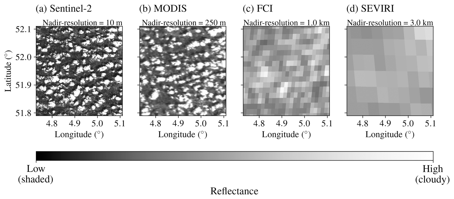
Figure 1 Measured reflectance on 3 July 2025 using channels near 0.6  µm from (a) Sentinel-2, (b) MODIS, (c) FCI and, (d) SEVIRI, for a domain comparable to the domain in this study. The measurements were performed at 10:50 UTC and for MODIS at 09:50 UTC. Reflectance has been normalised to yield the same average for all imagers.

Depending on the spatial scale, retrieval accuracy is influenced by a varying degree of sub-pixel variability and horizontal photon transport. Since measurements from individual passive imagers do not give information on sub-pixel variability and vertical cloud structure, it remains impossible from these observations alone to quantify exactly how 3D radiative effects and sub-pixel cloud heterogeneity influence GHI retrievals. The purpose of the present study is to understand the influence of spatial resolution and 3D radiative effects on GHI retrieval accuracy, a topic that has remained largely unexplored until now. Therefore, in this study, we employ highly accurate 3D RT simulations, at resolutions much finer than the current generation of geostationary satellites. This enables us to study how retrieval accuracy is influenced by spatial resolution, cloud variability, and 3D radiative effects. A better understanding of GHI retrieval errors should contribute to improving the quality of GHI nowcasts, especially for the most variable conditions that generally have the highest uncertainties (Wiltink et al., 2024).

We quantify the resolution dependence of GHI retrieval errors due to 3D RT for two highly variable shallow cumulus cloud fields at a range of resolutions increasing from 0.05 to 12.8 km. To do so, large eddy simulations (LES) are combined with satellite retrievals. The satellite retrieval is applied to synthetic top-of-atmosphere (TOA) reflectances simulated using the Monte Carlo KNMI (MONKI) radiative transfer code (Trees et al., 2025). As reference, GHI is also directly simulated from LES using the Monte Carlo raytracer that is part of the RTE-RRTMGP-CPP code (Veerman et al., 2022). The simulations of TOA reflectance and reference GHI are performed either based on 1D or 3D RT. The comparison of the various GHI fields enables us to evaluate the validity of the IPA and PPA at a range of spatial resolutions.

This article is structured as follows. Section 2 introduces the LES data of the shallow cumulus cloud fields, which serve as the basis for further analysis. The codes for LES, generating synthetic TOA reflectances, and for satellite retrieval are presented in Sect. 3, along with a more in-depth description of the methods used. The results are presented in Sect. 4 and further discussed in Sect. 5. Finally, the conclusions and outlook are given in Sect. 6.

2 Data

2.1 LES scene input data

This study uses the LES data of two shallow cumulus cloud fields forming the basis for the synthetic satellite retrievals. The chosen LES scenes originate from the study of Tijhuis et al. (2024), and are described in detail therein. Here, we only recap the essential settings relevant for this study and elaborate on the simplifications that have been made to the input.

The LES has been performed using MicroHH (van Heerwaarden et al., 2017). The full model setup for the current study can be found in Tijhuis (2024). In MicroHH radiation is solved in 1D using RTE-RRTMPG (Radiative Transfer for Energetics + RRTM for General circulations model applications–Parallel; Pincus et al., 2019) or in 3D using the raytracer of Veerman et al. (2022) (see Sect. 3.3). The initial and boundary conditions are based on ERA5 (Hersbach et al., 2020) and have been derived using LS2D (van Stratum et al., 2023). The horizontal size of the domain is 25.6 × 25.6 km with a resolution of 50 m. Vertically, the model extends up to 6.4 km with a resolution of 25 m. MicroHH accounts for the impact on radiation of gases located above the domain top by computing radiation in a single column that extends up to the top of the atmosphere.

The first of the two selected scenes is taken on 25 March 2014 at 12:00 UTC. The scene is characterised by a broken cumulus cloud field over grasslands, which is representative of the area around the Cabauw measurement tower in the Netherlands (51.4° N 4.9° E). The cloud cover of the scene is 22 %. The cloud base and cloud top heights, as determined from the lowest and highest level with a non-zero liquid water content, vary over the domain. The domain-averaged cloud base and top heights are 1550 and 1867 m, respectively. At 12:00 UTC the Sun is approximately south (the solar azimuth angle is 184.2°, measured clockwise from the North) with a solar zenith angle of 50.53°. In the remainder of the article, these values will be presented rounded to the nearest integer.

The second LES scene is taken on 4 May 2016 at 14:00 UTC, for the same domain as scene 1. Compared to the first scene, there is a higher cloud cover of 64 %. Compared to scene 1, the domain-averaged cloud base and cloud top are slightly higher, at 1884 and 2126 m, respectively. For a better comparison between scenes, we chose to stick to the solar geometry of scene 1, and also use the same background profiles of temperature, pressure, and ozone. Hence, the only model variables adjusted for scene 2 are the cloud properties r_e and liquid water path (LWP) and the water vapour content. Both scenes consists fully of water phase cloud droplets.

To make the LES data consistent with the assumptions made in the code to simulate TOA reflectances (i.e. MONKI, see Sect. 3.1) and the satellite retrieval (i.e. CPP-SICCS, see Sect. 3.2), some simplifications have been made to the original LES scenes.

First, in the original, realistic, LES scenes of Tijhuis et al. (2024) aerosols are included. Because we want to limit the study to 3D cloud effects only, all aerosols are excluded from the simulation. Concerning gases in the atmosphere, in MONKI, we only assume ozone as an absorbing gas, relevant at 0.640 µm, the visible (VIS) wavelength of the simulation. In the satellite retrieval, the effects of water vapour and CO₂ on GHI are included in addition to ozone. All other gases in the LES data are ignored.

To be consistent with the satellite retrieval, mid-latitude summer atmospheric profiles from Anderson et al. (1986) are assumed for ozone, pressure, and temperature instead of the original profiles from the LES scenes. Furthermore, the cloud droplet effective radii of the scene have been rounded to their nearest integer values, in order to align them to the droplet sizes used in MONKI (see Sect. 3.1). Finally, based on LES data a cloud mask is defined by LWP > 0 kg m⁻².

3 Methods

The methodology is subdivided into five subsections. First, the algorithm to generate synthetic TOA reflectances is introduced (Sect. 3.1). Then, in Sect. 3.2, the satellite retrieval is described. Section 3.3 introduces the raytracer used to compute 1D and 3D GHI directly from the LES cloud fields. In Sect. 3.4 the settings for additional sensitivity simulations are described. Finally, in Sect. 3.5 we present the methodology for separating the total error into various components.

3.1 TOA reflectance simulation

To create synthetic data satellite retrievals of TOA reflectance, the accurate and thoroughly validated 3D radiative transfer code Monte Carlo KNMI (MONKI; Trees et al., 2025) is used. MONKI can simulate Rayleigh scattering by gases, Mie scattering by clouds, gaseous and cloud absorption and Lambertian surface reflection, fully taking into account polarisation of light for all orders of scattering. For Earth-based applications, the optical properties of MONKI are identical to Doubling Adding KNMI (DAK), the RT code that is used by the satellite retrieval (de Haan et al., 1987; Stammes, 2001, see Sect. 3.2). To enable retrieval of cloud properties and GHI, TOA reflectances are simulated with MONKI at wavelengths of 0.640 and 1.625 µm. These wavelengths correspond to respective SEVIRI VIS/near-infrared (NIR) channels and allow for bispectral retrieval of cloud properties (Nakajima and King, 1990). In contrast to the actual reflectances from SEVIRI, which cover a narrow spectral band, the MONKI reflectances are fully monochromatic.

The MONKI simulations are performed using 10⁵ photons per column. In the simulations, the 3D state of the atmosphere is considered, and in addition to total radiative intensity, linear polarization is taken into account. MONKI simulations require atmospheric profiles for temperature, pressure, and ozone volume mixing ratios, for which mid-latitude summer profiles are assumed (Anderson et al., 1986). Furthermore, MONKI requires the cloud optical depth (τ) and effective cloud droplet radius (r_e) in µm for each cloudy grid cell. τ has been derived from the LES data using the liquid water path (LWP) in kg m⁻² and r_e in m, following Stephens (1978):

$$\begin{array}{}\text{(1)}& \mathit{\tau }={\displaystyle \frac{\mathrm{3}}{\mathrm{4}}}{Q}_{\mathrm{ext}}{\displaystyle \frac{\mathrm{LWP}}{{\mathit{\rho }}_{\mathrm{liq}}{r}_{\mathrm{e}}}}.\end{array}$$

Here, the liquid water density (ρ_liq) is 10³ kg m⁻³, and Q_ext represents the wavelength-dependent extinction efficiency, a unitless quantity derived from Mie theory, with a value close to 2. The range of available r_e in the current MONKI simulations is 3 to 22 µm in steps of 1 µm. This step size was used since including droplet sizes with smaller steps would make the MONKI simulations computationally unfeasible. However, for the current scenes all r_e are between 3 and 11 µm. Finally, per r_e, MONKI requires information on scattering properties, which has been generated with version 3.1 of the Meerhof Mie Program (de Rooij and van der Stap, 1984), using a two-parameter gamma droplet size distribution with an effective variance of 0.10.

In addition to the solar angles prescribed in the LES data file, MONKI requires information on satellite viewing and zenith angle. In the current simulations, a satellite viewing angle of 0° is used. For geostationary satellites observing the mid-latitudes, a nadir satellite viewing angle is not realistic. However, at slanted viewing angles, retrievals will be increasingly affected by parallax. The reference simulations are independent of viewing angle and therefore not influenced by parallax. Using a viewing zenith angle of 0° ensures that the retrieval does not require corrections for parallax, which would cause additional uncertainties. Note that for polar orbiting satellites such as MODIS, nadir viewing angles can be valid for the selected latitudes.

3.2 GHI retrieval

To retrieve GHI from synthetic MONKI simulated TOA reflectances, a two-step approach is followed. First, τ and r_e are retrieved using the Cloud Physical Properties (CPP) algorithm (Benas et al., 2023), which matches the synthetic VIS and NIR reflectances to simulated reflectances of homogeneous clouds, generated with DAK and stored in look-up tables (LUTs). Since the cloud field fully consists of water-phase clouds, only water clouds are considered in the retrieval. As mentioned in Sect. 3.1, the MONKI simulations are fully monochromatic, including only absorption by ozone, and the cloud property retrievals are performed correspondingly. Pixels are flagged as cloudy if the retrieved τ is above zero. Note that this internal retrieval cloud mask differs from the LES based cloud mask.

The second step is the retrieval of GHI using the Solar Irradiance under Clear and Cloudy Skies (SICCS) algorithm (Greuell et al., 2013). SICCS is based on radiative transfer simulations with a broadband version of DAK (Munneke et al., 2008) covering the spectral range 0.240 to 4.606 µm and using the correlated k-distribution technique to account for atmospheric gas absorptions. Cloudy-sky GHI is calculated for all cloudy pixels, and clear-sky GHI is calculated for all pixels.

In line with the MONKI simulations, no aerosols are included in these retrievals. Note that the atmosphere in DAK is plane-parallel, so the retrieved GHI with CPP-SICCS does not include 3D cloud effects.

As input, CPP-SICCS requires the cosine of the solar and satellite zenith angles, the relative azimuth between the Sun and the satellite, the surface albedo for both the VIS and NIR channels, the water vapour column per pixel in kg m⁻², and the ozone concentration in Dobson units (DU). In the retrieval the ozone concentration is fixed at 332 DU, which is a typical value for the mid-latitudes in summer and the same as used in the MONKI simulations.

3.3 Reference GHI

In addition to GHI retrieved from the simulated TOA MONKI reflectances and the CPP-SICCS algorithm, GHI is also computed directly from the LES data using a Monte Carlo Raytracer (hereafter, MCRT; Veerman et al., 2022). MCRT is an extension of the C$++$/CUDA implementation of the 1D RT model RTE-RRTMPG. In contrast to the CPP-SICCS satellite retrieval, where the atmosphere is plane-parallel and the different columns are independent, MCRT enables the simulation of both 1D, that is, assuming plane-parallel and independent pixels, as well as full 3D RT. The version of MCRT employed in this study uses another set of Mie look-up tables (Prahl, 2025) to determine the scattering directions for water clouds with an r_e between 3–22 µm in steps of 1 µm. To compute broadband fluxes, the raytracing is performed independently over 14 wavelength bands, each containing 224 quadrature points. The total spectral width covered by MCRT ranges from 0.2 to 12.2 µm. which is broader than for the satellite retrieval. However, since the spectral differences occur at the edges of the solar spectrum where a negligible amount of solar radiation is received, this results in negligible differences in broadband GHI. In this study, MCRT is run using 1024 samples per pixel per quadrature point.

3.4 Scenarios

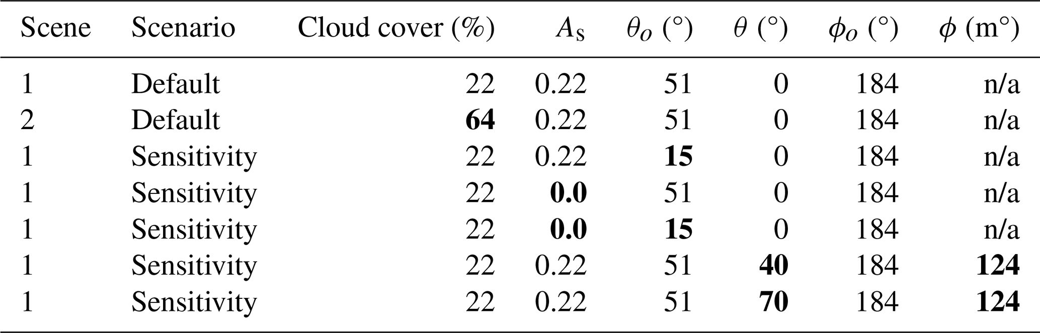
In addition to the simulations of the two default scenes introduced in Sect. 2, five additional sensitivity experiments are performed for the scene with low cloud cover (Scene 1). With the first sensitivity test, the importance of changes in surface albedo is studied by using a surface albedo of zero (black surface) instead of the default value of 0.22. In the second sensitivity experiment the influence of solar zenith angle (θ₀) variations is studied by reducing θ₀ from 51° to 15°. The third experiment combines adjustments of the previous two sensitivity tests. The last two sensitivity experiments are aimed at the influence of the viewing zenith angle (θ) on retrieval accuracy. In this experiment the satellite position is changed to a satellite viewing angle of 40° or 70° with a relative azimuth of 60° between the Sun and the satellite. An overview of the used geometry and surface albedo for various simulations is presented in Table 1. Hereafter, we will refer to the simulations with different geometries or surface albedo as scenarios.

Table 1 Overview of the surface albedo (A_s), solar zenith angle (θ_o), satellite viewing zenith angle (θ), solar azimuth angle (ϕ_o) and the satellite azimuth angle (ϕ) used for the simulation of the scenes with low and high cloud cover. The azimuth angles are defined from 0° North and increase clockwise. The parameters that have been adjusted with respect to the default scenario of scene 1 are indicated in bold. “n/a” means “not applicable”.

3.5 GHI simulation pathways and error separation

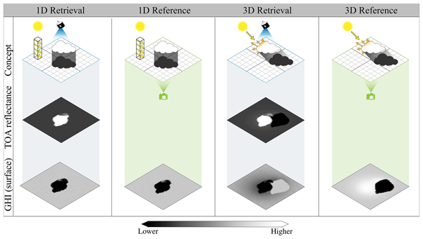
To study the influence of spatial resolution and 3D cloud effects on GHI retrieval accuracy, we retrieve and simulate GHI using four main pathways, shown graphically in the flow chart of Fig. 2. In the retrieval pathways, MONKI is used to simulate TOA reflectances that serve as input for the CPP-SICCS GHI retrieval (Top pathways of Fig. 2). In the reference pathways, MCRT is used to directly compute GHI from the LES scene (bottom pathways of Fig. 2). To be able to isolate 3D cloud effects, both MCRT and MONKI are run using 3D RT and 1D RT, i.e., assuming independent pixels. This results in four GHI fields per scenario as summarised in Table 2. The four pathways are also conceptually illustrated in Fig. 3.

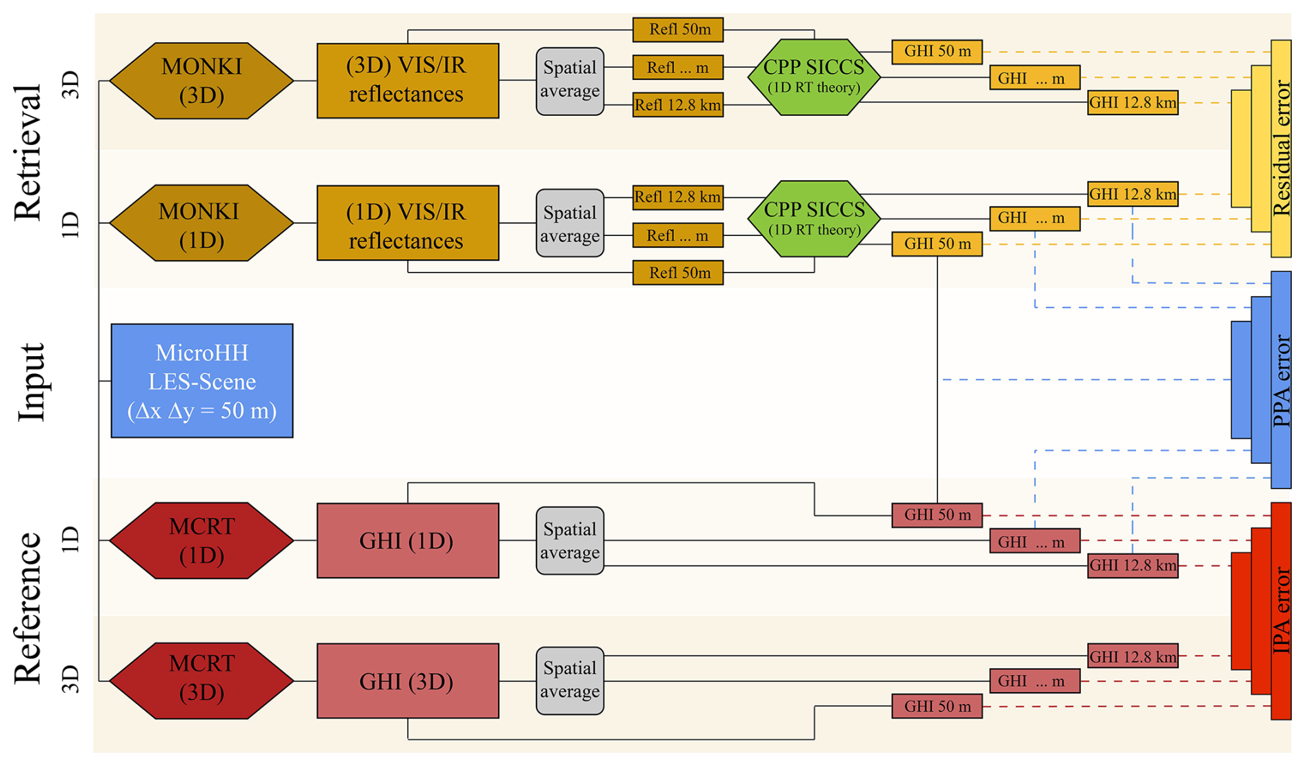
Figure 2 Flow diagram summarising the various steps of the methodology to retrieve and simulate GHI based on 1D or 3D RT and to break down the errors into PPA, IPA, and residual contributions. The rectangles represent data products while the hexagons refer to the various codes used in this study. The dotted lines indicate which data products are compared to get the PPA, IPA, and residual errors.

Table 2 Summary of the algorithms and definition of the atmosphere (3D or IPA) used to generate the four GHI fields for each scenario. “n/a” means “not applicable”.

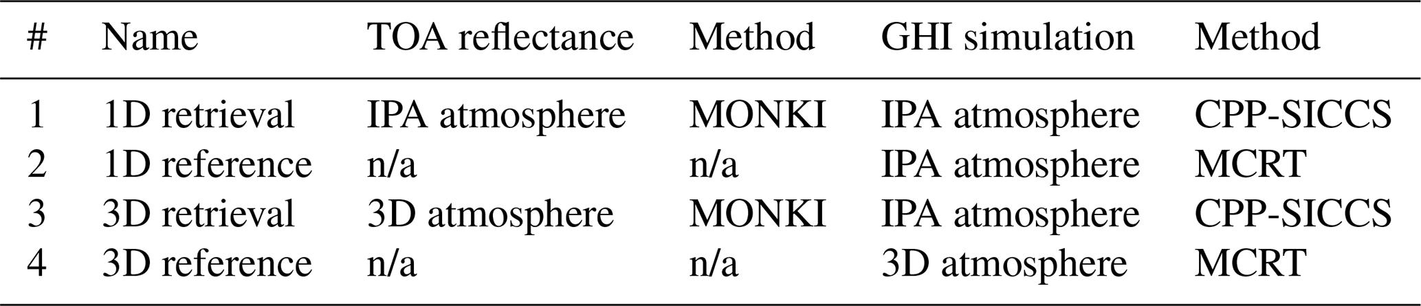
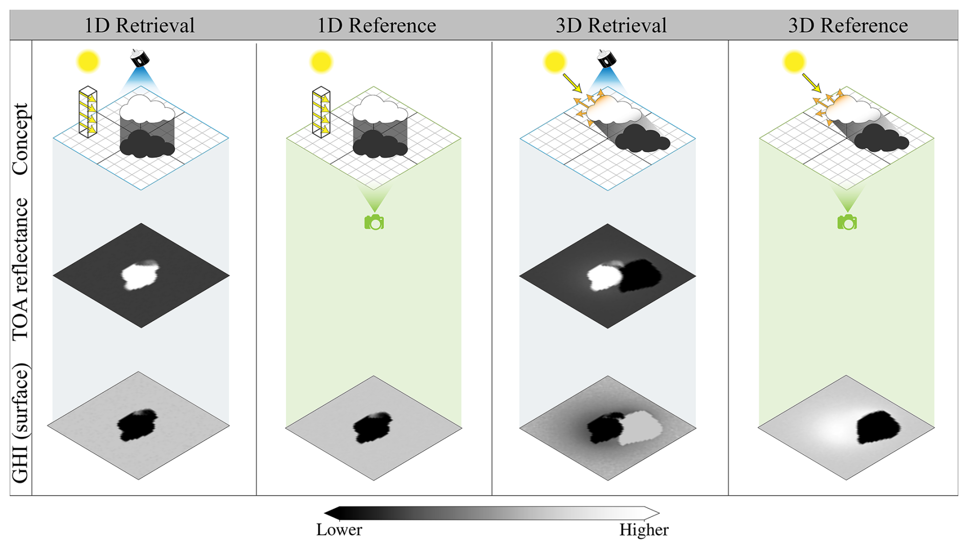
Figure 3 Conceptual images (top row) illustrating the deviations between the four pathways to retrieve or simulate GHI. Below the conceptual images the spatial distributions of the simulated TOA reflectance (middle row, retrieval only) and retrieved/simulated GHI (bottom row) are shown for a single isolated cloud.

Next, to study the effects of spatial resolution on retrieval accuracy, the 0.05 km pixel sizes of the original LES scene are spatially averaged by a factor 2 using box-averaging, as shown by the square boxes in Fig. 2. Spatial averaging is repeated multiple times to assess retrieval accuracy at 9 different spatial resolutions, namely: 0.05, 0.1, 0.2, 0.4, 0.8, 1.6, 3.2, 6.4, and 12.8 km. Note that for the reference pathway the GHI output is spatially averaged. However, for the retrieval pathway we do not average GHI but rather the MONKI TOA reflectances and perform the satellite retrieval based on the averaged reflectances. For the retrieval, averaging the reflectances is representative of what a real instrument would measure at the selected spatial resolution.

At each resolution, the errors between the retrieval and the reference can be separated into various components. First, the error resulting from the IPA can be derived from the comparison of the 1D reference GHI with the 3D reference GHI, as indicated by the vertical rectangles in the bottom right of Fig. 2. The IPA error is caused by the neglect of 3D RT.

Next, the PPA error can be quantified by comparing the 1D retrieval to the 1D reference (shown by the vertical rectangles in the middle right of Fig. 2). The PPA error is introduced by spatial averaging of reflectances in the satellite retrieval. Since both 1D pathways are fully plane-parallel within each pixel and the IPA is used, 3D radiative effects are not present, and thus the error must originate from ignoring the sub-pixel variability. At the original spatial resolution of 0.05 km, no spatial averaging is performed, and therefore the corresponding PPA error should be 0. This is only valid in case the MCRT reference simulation and the MONKI + CPP-SICCS satellite retrieval are consistent. In Sect. 4.1 the consistency of the models is validated. Note that potential sub-pixel variability at spatial scales finer than 0.05 km cannot be captured by our simulations but does occur within real cloud fields. We neglect potential sub-pixel cloud variability at spatial scales finer than 0.05 km.

Finally, we identify a residual error from the comparison between the 3D retrieval and the 1D retrieval. In Fig. 2 this is illustrated by the vertical rectangles in the upper right corner. This residual error can be explained as follows. In the 1D retrieval both the simulation of reflectances and retrieval of GHI are performed relying on the IPA, which makes these steps fully consistent. For the 3D retrieval, independent pixels are assumed in the GHI retrieval step but not for the simulation of TOA reflectance, which is fully 3D. As a result, inconsistencies between the simulation of reflectances (with MONKI) and retrieval of GHI (with CPP-SICCS) are introduced.

In the current study, we quantify errors using the bias and root mean square error (RMSE) as evaluation metrics. Equation 2 shows for the bias how the three components of the error can be derived from the pathways noted in Table 2 and shown in Fig. 2 and how they add up to the total bias,

$$\begin{array}{}\text{(2)}& \begin{array}{rl}\underset{\mathrm{Totalbias}}{\underbrace{({\mathrm{GHI}}_{\mathrm{Retrieval}}^{\mathrm{3}\mathrm{D}}-{\mathrm{GHI}}_{\mathrm{Reference}}^{\mathrm{3}\mathrm{D}})}}& =\underset{\text{IPA bias}}{\underbrace{({\mathrm{GHI}}_{\mathrm{Reference}}^{\mathrm{1}\mathrm{D}}-{\mathrm{GHI}}_{\mathrm{Reference}}^{\mathrm{3}\mathrm{D}})}}\\ & +\underset{\text{PPA bias}}{\underbrace{({\mathrm{GHI}}_{\mathrm{Retrieval}}^{\mathrm{1}\mathrm{D}}-{\mathrm{GHI}}_{\text{Reference}}^{\mathrm{1}\mathrm{D}})}}\\ & +\underset{\text{Residual bias}}{\underbrace{({\mathrm{GHI}}_{\mathrm{Retrieval}}^{\mathrm{3}\mathrm{D}}-{\mathrm{GHI}}_{\mathrm{Retrieval}}^{\mathrm{1}\mathrm{D}})}}.\end{array}\end{array}$$

4 Results

In this section, first, the agreement between the MCRT reference and satellite retrieval is validated (Sect. 4.1). Next, results are presented for the cloud fields with low and high cloud cover (Sect. 4.2 and 4.3, respectively).

4.1 Validation

To rule out inconsistencies between the forward radiative transfer models (MONKI and MCRT) and the retrieval codes (CPP-SICCS), a validation is performed for cloud properties and GHI based on the 1D retrieval and 1D reference at a spatial resolution of 0.05 km.

4.1.1 Validation of cloud properties

The first step in the validation is a comparison of the retrieved cloud properties against the LES data. Figure 4 shows histograms of the 1D-retrieved τ and r_e compared to the LES data for the two scenes. The results are presented for the default scenarios (see Table 1), but the results for other configurations are comparable.

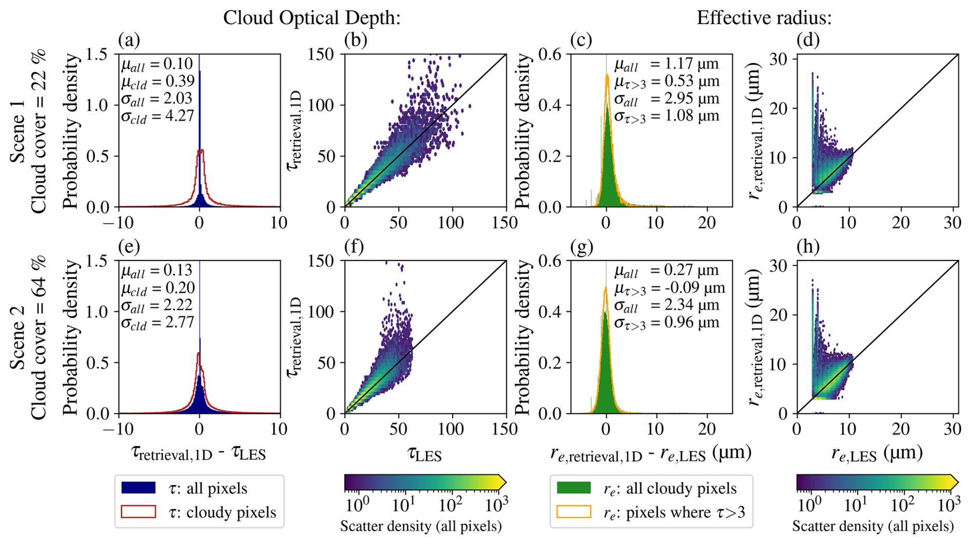
Figure 4 Validation of the 1D retrieved τ (a, b, e, f) and r_e (c, d, g, h) against the LES data for scene 1 (a–d) and scene 2 (e–h). The histograms and scatter density plots are shown for the default scenario specified in Table 1. The distinction between τ: all pixels and τ: cloudy pixels is based on the liquid water path from the LES data. The CPP-SICCS retrieval can retrieve small non-zero optical depths for clear-sky pixels, explaining the difference between τ: all pixels and τ: cloudy pixels.

The retrieved τ agrees well with the τ from the LES data; the mean bias for cloudy pixels is below 0.4. Still, towards higher τ an overestimation of the retrieved τ can be observed especially in Scene 2. This illustrates the increased absolute uncertainty in the τ retrieval for optically thick pixels (Platnick et al., 2017). Note that the share of these pixels is very limited and therefore the weight on the overall bias is limited. Furthermore, the histogram of the τ differences shows some spread, but this can mainly be attributed to model noise arising from the Monte Carlo simulations with MONKI.

The retrieved effective radii are representative for the upper portion of the clouds, as indicated by vertical weighting functions presented in Platnick (2000). To reflect this, the vertical r_e profiles are converted to column values by applying an exponentially decreasing weight from the top down into the cloud, with a decay scale of 10 (optical thickness units). The r_e retrievals show small positive biases especially for scene 1. A considerable part of this bias is due to the uncertainty in the r_e retrieval for thin clouds. For optically thicker clouds (with τ > 3) there is a better agreement between the LES and the retrieval. Overall, the validation of cloud properties gives the confidence that there are no major systematic biases introduced by the simulation of TOA reflectances with MONKI and the cloud property retrieval of CPP.

4.1.2 Validation of GHI

The 1D retrieved GHI is validated against the 1D MCRT reference in Fig. 5. For cloudy pixels, the biases are slightly positive in both scenes (Fig. 5a, c). The mean GHI of the 1D retrieval is about 2 W m⁻² higher than the 1D reference. The retrieval tends to underestimate GHI at low values, which is consistent with the overestimation of τ for thick clouds in Fig. 4.

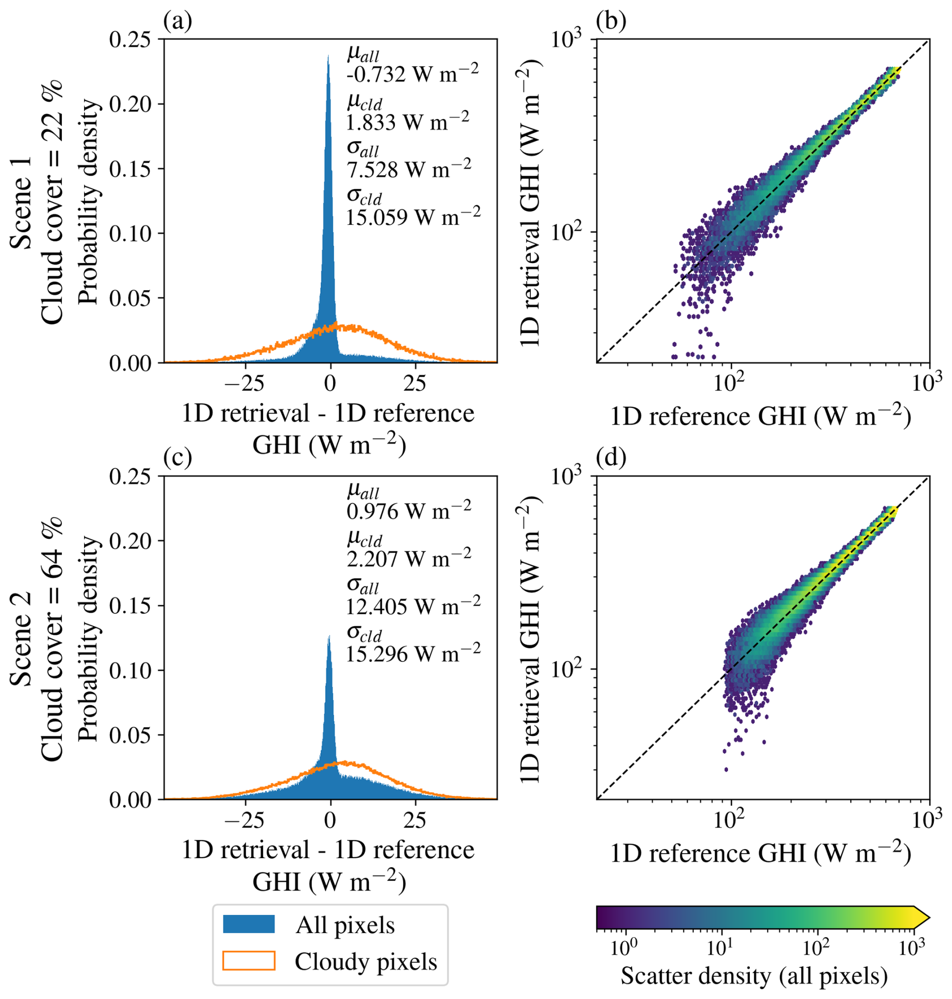
Figure 5 Validation of the 1D retrieved GHI against the 1D reference GHI from MCRT for scene 1 (a, b) and 2 (c, d). Results are presented for the same scenarios as in Fig. 4.

Meanwhile, there is a slightly negative clear-sky bias for both scenes, which can be seen from the distribution around the peaks in the probability density functions (PDF) for all-sky conditions. The negative bias can be explained by the remaining noise in the simulated TOA reflectances. Consider a clear-sky pixel, i.e., a pixel with a reflectance exactly equal to the clear-sky reflectance. Now, if some positive noise is added, the reflectance will be elevated above its clear-sky value. The pixel will be retrieved as if it contains a thin cloud, and hence the GHI is lowered compared to the clear-sky value. If the same noise is subtracted from the the reflectance it will be lower than the clear-sky value, and thus the pixel will be retrieved as clear-sky. The GHI will then equal the retrieved value in the absence of noise.

The all-sky bias is the result of a positive cloudy-sky and negative clear-sky bias. It is negative for scene 1 but positive for scene 2, which can mainly be attributed to the higher cloud cover for scene 2.

All in all, the model biases from this validation are more than an order of magnitude smaller than the total bias between retrieval and reference (see Sect. 4.2). Therefore, we deem the GHI biases between retrieval and reference small enough to continue the analysis.

4.2 Scene 1: low cloud cover

4.2.1 Spatial distribution of GHI

In this section, we present the results of the impact of various spatial resolutions on the GHI retrieval. First, we examine the spatial distribution of the GHI fields for the 1D retrieval and 1D reference using the IPA (top two rows of Fig. 6). At a 0.05 km spatial resolution, nearly identical irradiance fields are shown. From these spatial plots two distinct areas can be identified. On the one hand, clear-sky regions receiving high GHI and on the other hand regions where, depending on τ, GHI is reduced because clouds block the sunlight reaching the surface. The strict separation is caused by the absence of horizontal transport of photons. The close correspondence between the 1D reference and 1D retrieval at 0.05 km was already demonstrated in Sect. 4.1.2. Interestingly, towards coarser spatial resolutions, there is a growing deviation in GHI between the 1D reference and the 1D retrieval, resulting from stronger GHI reductions for the 1D retrieval. This is due to the mixing of the reflectances of clear-sky and cloudy pixels (hereafter called clear-cloudy mixing). The implications of clear-cloudy mixing are discussed in detail in Sect. 5.1. In short, when clear-sky pixels or pixels with a low cloud optical depth (τ ≲ 5) are mixed with cloudy pixels with a higher τ, a transmittance bias is introduced.

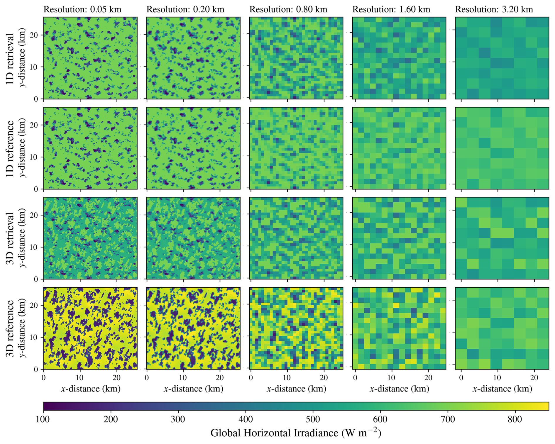
Figure 6 Spatial plots of GHI for scene 1 generated using the 1D retrieval (top row), 1D reference (second row), the 3D retrieval (third row) and 3D reference (bottom row) at decreasing spatial resolutions from 0.05 km (leftmost column) to 3.2 km (rightmost column). Results are presented for the default scenario of scene 1.

Next, we take a closer look at the spatial GHI distributions of the full 3D reference (bottom row of Fig. 6). At the finest spatial resolutions, there are distinct differences between the 3D reference and the 1D retrieval and reference GHI fields (top 2 rows of Fig. 6). As a first observation, for the 3D reference, displacement of cloud shaded regions is shown with respect to the 1D projected shadow locations. Furthermore, in between the cloud shaded areas, the majority of pixels receive irradiance which is higher than the clear-sky value. These areas correspond to irradiance enhanced pixels receiving scattered radiation from adjacent clouds in addition to direct radiation from the Sun.

Considering the GHI of the 3D retrieval (third row of Fig. 6) at resolutions of 0.05 km, visually large deviations are apparent between the 3D retrieval and the 3D reference. We can roughly identify three distinct regions in the 3D retrieved GHI field. Firstly, just as for the 1D retrieval and 1D reference, we can identify the pixels that are directly located below the clouds as the pixels with often strong reductions in GHI. Secondly, regions are identified where irradiance enhancements occur. However, in the 3D retrieval, these regions are not characterised by an increase in GHI with respect to the clear-sky value as is the case for the 3D reference, but rather by a slight decrease in GHI of around 150 W m⁻². This decrease in GHI is explained in the following way. The simulations of TOA reflectance for the 3D retrieval are fully 3D and, therefore, enable increases in reflectance due to irradiance enhancement (not shown). However, for the 3D retrieval of GHI the satellite retrieval still assumes an IPA atmosphere in which irradiance enhancements cannot be resolved. Since irradiance enhancements are characterised by an increase in reflectance with respect to clear-sky, the GHI satellite retrieval incorrectly flags these pixels as being cloudy. Hereafter, we call this effect the retrieval error due to irradiance enhancement. Finally, cloud shaded pixels can be identified. In the retrieval, the cloud shaded regions counterintuitively and incorrectly correspond to the regions where GHI has a clear-sky value. This can be explained by the opposite mechanism to the retrieval error due to irradiance enhancement. In the simulation of TOA reflectance, due to horizontal photon transport, cloud-shadows have a reflectance which is below that of the clear-sky reflectance. Since the satellite retrieval does not account for horizontal photon transport, in the retrieval, a reflectance that is below the clear-sky value will result in a clear-sky GHI flux.

Despite the large local differences observed in the spatial plots of GHI at the finest resolutions (Fig. 6), when spatial averaging is performed, these differences are smoothed out, and deviations between the 3D and 1D retrievals and reference become less extreme.

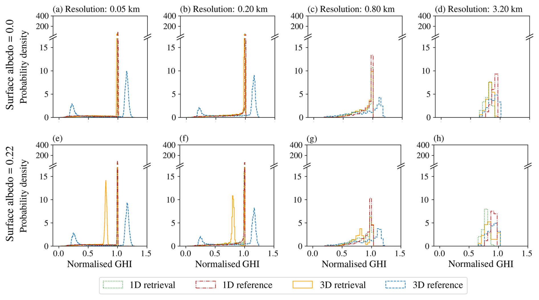
Figure 7 PDFs of the normalised 1D and 3D retrieved and reference GHI, at varying spatial resolutions. Normalization has been performed with the reference clear-sky GHI. The results are presented for scene 1 for the scenarios with a θ₀ of 51° and a surface albedo of 0.0 (a–d) or 0.22 (e–h).

4.2.2 Probability density distribution of GHI

To better illustrate the impact of spatial averaging on the GHI distribution, PDFs of normalised GHI are plotted at decreasing spatial resolution and for two surface albedos (Fig. 7). The GHI distributions are normalised by the 3D reference clear-sky GHI. The PDFs illustrate that at the finest spatial resolutions, the 3D reference GHI has a clear bimodal distribution (dashed line in Fig. 7a, e), which is characteristic of situations with broken or shallow cumulus clouds (Gristey et al., 2020; Tijhuis et al., 2024). In this bimodal distribution, the small peak around a normalised GHI of 0.25 represents diffuse irradiance in cloud shaded regions. The larger peak around a normalised GHI of 1.15 corresponds to clear-sky regions where irradiance enhancement takes place.

Next, for the 1D retrieval (dotted lines in Fig. 7a, e) and 1D reference (dash-dotted lines in Fig. 7), due to the absence of cloud shadows and horizontal scattering, only one narrow peak in GHI at a normalised GHI of 1 occurs, corresponding to the clear-sky pixels. The occurrence frequency of a certain GHI value for the cloudy pixels is very low and the distribution is spread over a large range, depending on τ as noted in Sect. 4.2.1.

Third, for the 3D retrieval, clearly distinct PDFs can be observed between the surface albedos of 0.0 and 0.22 (solid lines in Fig. 7a, e). For both albedos, there is a peak at a normalised GHI of 1. Note that where this peak corresponds to clear-sky pixels for the 1D retrieval and 1D reference, for the 3D retrieval the peak is associated to cloud-shaded areas (see Sect. 4.2.1). The main difference between the two albedos lies in the additional peak in normalised GHI around 0.8 for the 3D retrieval with a surface albedo of 0.22 (Fig. 7e). This peak results from the retrieval error due to irradiance enhancement, where irradiance enhanced pixels are incorrectly retrieved as cloudy, thus reducing GHI. The fact that the peak seems to be absent in case of a surface albedo of 0.0 can be explained through a mechanism called albedo enhancement (Mol and van Heerwaarden, 2025) or more broadly entrapment, when it takes place for scatterers other than the surface (Schäfer et al., 2016; Hogan et al., 2019). Surface albedo can cause irradiance enhancements through multiple iterations of scattering between the surface and cloud base. This effect becomes more effective at higher surface albedo (for instance, over snow covered surfaces) and at increasing cloud cover. In case of a black surface, all photons that hit the surface are absorbed and there is no albedo enhancement. Without the contribution of the albedo enhancement, the magnitude of the irradiance enhancements remains more limited. Still, even with surface albedo of 0.0, irradiance enhancements are not fully absent. Horizontally scattered photons that do not hit the surface can still contribute to an increase in reflectance. Close inspection of the PDF of the 3D retrieval for a surface albedo of 0.0 (solid line in Fig. 7a) reveals that the second peak in normalised GHI is located just below 1.

Finally, toward coarser spatial resolutions the peak related to the retrieval error due to irradiance enhancement in Fig. 7e–g gradually disappears, as well as the bimodal distribution of the 3D GHI reference. At coarser resolutions, the results are converging towards the domain averaged GHI flux. Although at a spatial resolution of 3.2 km (Fig. 7d, h) the different GHI distributions look more similar in terms of shape than at a resolution of 0.05 km, the coarser resolutions also show deviations between the mean GHI of the retrievals and the reference, especially with a surface albedo of 0.22.

4.2.3 Domain-averaged GHI

The histograms of Fig. 7 show the GHI distribution for various spatial resolutions but do not directly indicate the effects of spatial resolution on domain-averaged GHI fluxes. Therefore, this section will focus on the domain averaged fluxes of the various scenarios of scene 1 (Fig. 8). The absolute magnitude of GHI strongly depends on θ₀. For a better comparison between the low sun and high sun scenarios, we again normalise the GHI fluxes with the respective 3D reference clear-sky flux.

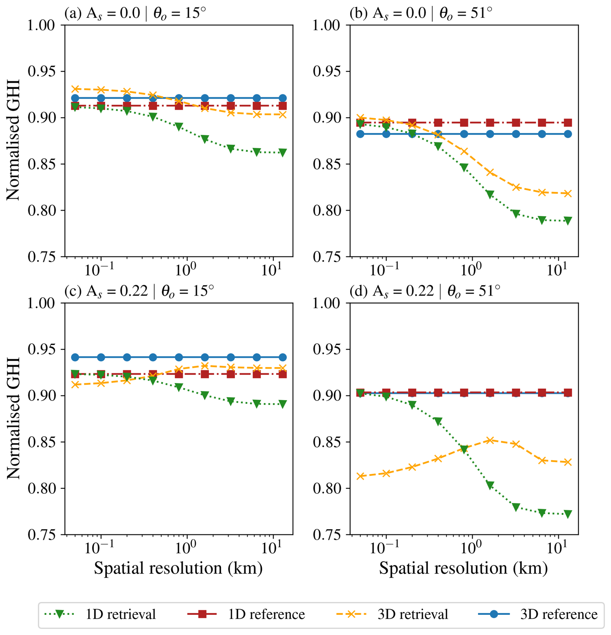
Figure 8 Domain-averaged GHI normalised with the 3D reference clear-sky GHI as function of spatial resolution. The scenarios shown are: A_s=0.0 (top row), A_s=0.22 (bottom row), θ₀=15° (left column) and θ₀=51° (right column), all for scene 1.

From Fig. 8, several messages are conveyed. First, it becomes apparent that for the 1D (square markers) and 3D (round markers) reference, the domain-averaged GHI does not depend on spatial resolution. This is as expected since regardless of the spatial resolution, the amount of radiation remains preserved within the domain.

In contrast, for both the 1D and 3D retrievals, the domain-averaged GHI does depend on resolution. This is because of the non-linear relation between observed TOA reflectance (of which the domain average is preserved at varying resolution) and retrieved GHI. At 0.05 km resolution the agreement between the 1D retrieval (triangular markers) and 1D reference was already demonstrated (see Sect. 4.1). However, towards coarser spatial resolutions, a decrease in 1D-retrieved GHI becomes apparent, regardless of the scenario. This decrease is attributed to the clear-cloudy mixing effect (see Sect. 5.1).

Moving on to the 3D retrieval (cross markers) it is shown that the GHI trends with spatial resolution strongly depend on the solar geometry and surface albedo of the respective scenario. We will first explain the trend in GHI for the default scenario (Fig. 8d). Initially, at 0.05 km resolution, the 3D retrieved normalised GHI is about 0.08 lower than the 3D reference. This is the result of the retrieval error due to irradiance enhancement that lowers the retrieved GHI of clear-sky pixels being more prominent than the retrieval error due to shading which causes GHI overestimation (see Sect. 4.2.1).

As the spatial resolution gets coarser, the GHI increases until a spatial resolution of 1.6 km. To understand this increase in GHI, we need to consider the balance between irradiance enhanced and shaded pixels. To this end, Fig. 9 shows the effective clear-sky fraction (round markers), irradiance enhancement fraction (cross markers) and cloud shadow fraction (square markers). The effective clear-sky fraction is derived from the cloud mask based on the LWP from the LES data. Here the term effective indicates that the fraction of pixels with LWP = 0 kg m⁻² depends on the spatial resolution, whereas the clear-sky fraction itself does not. The cloud shadow fraction is computed as the fraction of pixels that are clear-sky and located in the shadow of a cloud, where the shadow calculation is based on a geometrical formula using solar position and the cloud top height, following Wiltink et al. (2025a). Finally, the irradiance enhancement fraction is defined as the fraction of pixels for which the 0.64 µm reflectance of the 3D retrieval exceeds that of the 1D retrieval by a predefined threshold, here set to 3 % ± 1 %.

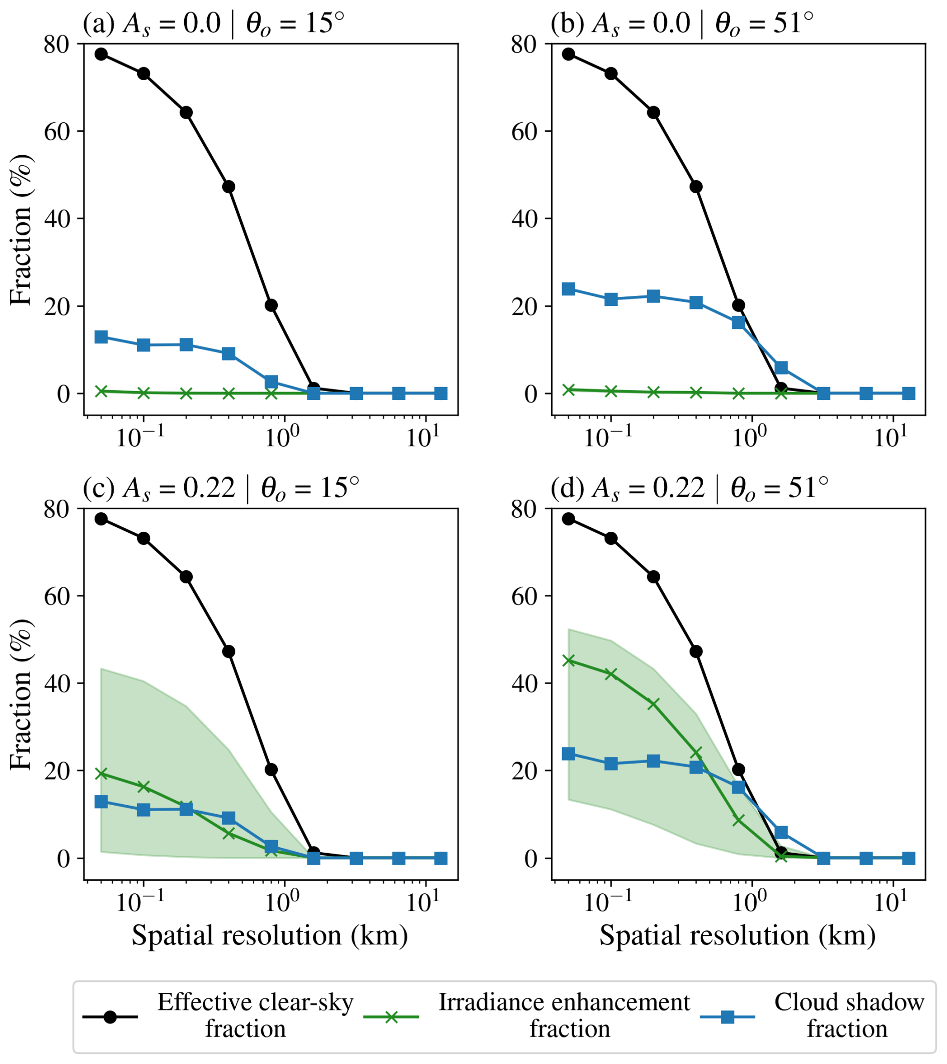
Figure 9 The effective clear-sky fraction, cloud shadow fraction and irradiance enhancement fraction as a function of spatial resolution. The magnitude of the irradiance enhancement fraction is shown for enhancements of 3 % (solid line) and 2 % to 4 % (shaded area). The scenarios shown are the same as in Fig. 8.

At the finest resolution, irradiance enhancements are the most prominent (cross markers in Fig. 9d). Towards coarser spatial resolutions, the total fraction of the irradiance enhanced pixels rapidly decreases. This is the result of a decrease in the effective clear-sky fraction (round markers in Fig. 9d). Note that the true cloud cover of the scene remains 22 % (Table 1) regardless of the spatial resolution. However, due to spatial averaging, clear and cloudy pixels get mixed, increasing the share of pixels flagged as cloudy. Since the share of irradiance enhanced pixels decreases, the magnitude of the error due to irradiance enhancement decreases as well. Meanwhile, it is shown that the cloud shadow fraction (square markers in Fig. 9d) remains constant until a spatial resolution of about 0.8 km and so does the retrieval error due to shading.

When resolutions get coarser, the underestimation in the retrieval due to irradiance enhancements disappears whereas the overestimation due to shadowing remains preserved. Therefore, a net increase in domain-averaged GHI is observed (cross markers in Fig. 8d). At a spatial resolution of around 1.6 km, the cloud shadow fraction becomes zero and therefore the increasing trend in domain-averaged bias levels off. Finally, at the coarsest resolutions, it is the clear-cloudy mixing that is dominant and causes a slight reduction in the domain-averaged GHI.

Continuing with the scenario with a θ₀ of 15° and a surface albedo of 0.22 (Fig. 8c). Here, both for the 1D and 3D retrieval, a trend similar to that of the default scenario is observed, yet, with a much smaller amplitude. For the 3D retrieval, the reason for this is threefold. First, both the irradiance enhancement fraction and magnitude, and therefore the corresponding retrieval error, at a θ₀ of 15° is smaller than at a θ₀ of 51° (compare cross markers and shaded areas between Fig. 9c and d). Information on the magnitude of irradiance enhancement can be derived from Fig. 9 by comparing the ratios of irradiance enhancement fractions, for instance, those of 3 % and 4 %. Relatively, there are much fewer pixels with enhancements exceeding 4 % for the high sun scenario than for the low sun scenario. Consequently, at a θ₀ of 15° the corresponding retrieval error is smaller than at a θ₀ of 51° and and the 0.05 km GHI is much closer to the reference. Furthermore, a higher sun means smaller cloud shadow displacements and smaller cloud shadow areas (square markers in Fig. 9c), and therefore, the increase in GHI towards coarser spatial resolutions remains more limited (i.e. smaller retrieval error due to shading). Finally, for spatial resolutions where the effective cloud fraction approaches 100 %, the reduction in GHI remains more limited due to the smaller clear-cloudy mixing errors at this lower solar zenith angle (see Sect. 5.1) The smaller amplitude in reduction of GHI for the 1D retrieval at 15°, is fully explained by the smaller clear-cloudy mixing.

Finally, for the retrievals with a black surface (cross markers and triangular in Fig. 8a, b), no increase in GHI is observed towards coarser resolution. Furthermore, unlike the retrievals with a surface albedo of 0.22, at the finest spatial resolutions, the domain-averaged GHI is higher than the reference.

To explain this, we again need to consider the reflectance for irradiance enhanced and cloud-shaded pixels. In the case of a surface albedo of 0.0, irradiance enhancements are practically absent (cross markers in Fig. 9a, b). Meanwhile we do identify a cloud shadow fraction (square markers in Fig. 9a, b), Correspondingly, there is only a retrieval error due to shading, and GHI is overestimated with respect to the reference. Towards coarser spatial resolutions, the GHI decreases because of the clear-cloudy mixing.

To summarise, despite the varying trends in domain-averaged GHI of the 3D retrieval towards coarser resolutions, in all cases the trends can be explained from the balance between the retrieval errors due to irradiance enhancement and shading as well as the effect of clear-cloudy mixing.

4.2.4 Error separation

In Fig. 10 we now continue to separate the domain-averaged GHI bias into the various components defined in Eq. (2). The bias trends are discussed per error component, starting with the errors associated with the IPA (triangular markers). Depending on the scenario, the domain-averaged IPA bias ranges between −20 and 10 W m⁻². Previous studies (Tijhuis et al., 2024) showed that for cumulus clouds in uncoupled LES simulations, generally, there is less direct radiation simulated when 3D RT is applied than when horizontally independent columns are assumed. Meanwhile, for diffuse and global radiation applying 3D RT instead of 1D RT results in higher fluxes (Gristey et al., 2020; Tijhuis et al., 2024). The negative IPA biases for GHI observed in this study agree well with these observations (triangular markers in Fig. 10a, c). However, the positive bias of around 10 W m⁻² observed for the scenario with a surface albedo of 0 and a θ₀ of 51° is remarkable (triangular markers in Fig. 10b). This deviation is mainly attributed to the surface albedo and the related albedo enhancement as described in Mol and van Heerwaarden (2025). With a surface albedo of 0 there is no albedo enhancement. Consequently, the increase in diffuse irradiance remains more limited and therefore allows for the larger observed positive biases in global radiation.

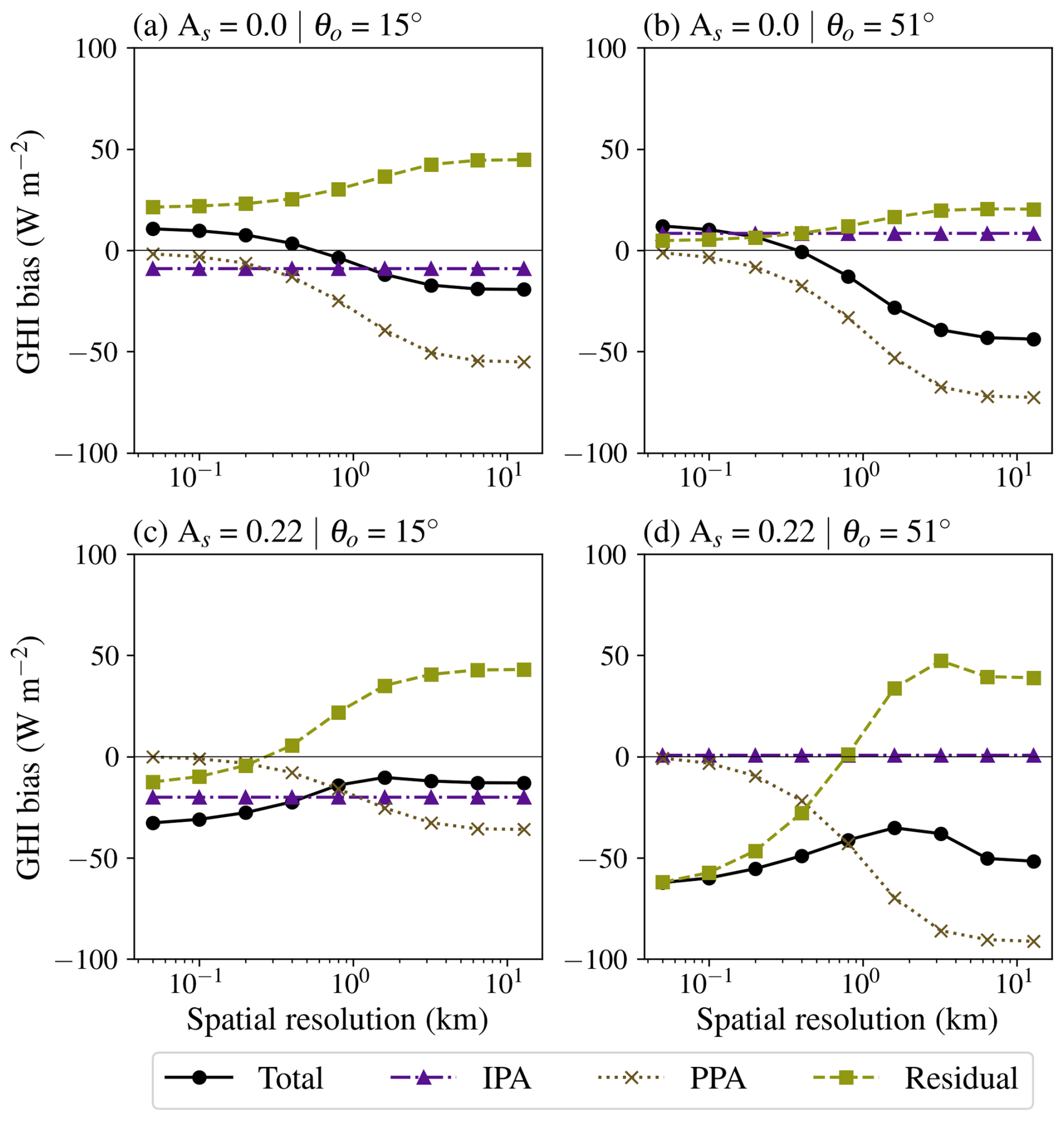
Figure 10 The total domain-averaged bias as function of spatial resolution and the biases separated into the contributions due to the PPA, IPA and residual errors. The scenarios shown are the same as in Fig. 8.

The PPA bias (cross markers in Fig 10) is around 0 W m⁻² at 50 m resolution for all scenarios. This is as expected, since by construction there is no sub-pixel variability at this scale. As the spatial resolution becomes coarser, the 1D reference GHI remains constant while due to clear-cloudy mixing, the GHI of the 1D retrieval decreases. Therefore, the observed PPA biases can be fully attributed to the error due to clear-cloudy mixing in the 1D retrieval. The observation that the error due to PPA increases towards coarser spatial resolutions is in line with previous findings by Zinner and Mayer (2006).

For the residual biases generally increasing trends are observed for the different scenarios (square markers, Fig 10). Each of these trends can be explained by the balancing between the retrieval error due to irradiance enhancement, the retrieval error due to shading and the error due to clear cloudy mixing and their relation with solar zenith angle and surface albedo at each of the spatial resolutions (see Sect. 4.2.3).

The total bias (round markers in Fig. 10) is the sum of the IPA, PPA and residual biases. For the scenarios in which the surface albedo is 0.22 (Fig. 10c, d), the smallest biases are found at a spatial resolution around 1 to 3 km. Towards a coarser spatial resolution, biases become more negative due to the PPA bias, while towards finer spatial resolutions, they become more negative due to the residual bias. For the scenarios with a surface albedo of 0.0, the residual bias is much smaller, and the total bias mainly varies as the PPA bias. The total biases start off positive and become negative towards coarser spatial resolutions. The bias changes sign around 0.4 (θ₀ = 51°) to 0.8 km (θ₀ = 15°).

Figure 11 Same as Fig. 10 but now for the RMSE.

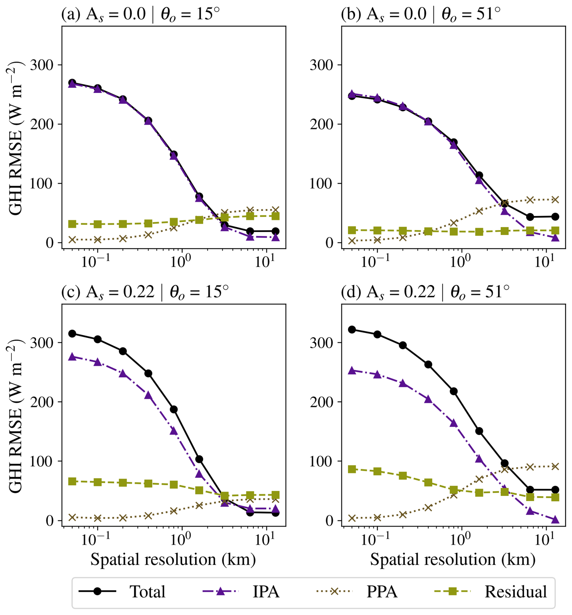
Although the IPA bias turns out to be rather small due to counteracting 3D radiative effects such as irradiance enhancement and shading, 3D radiative effects strongly influence local GHI errors as shown by the RMSE in Fig. 11. The RMSE shows that at a spatial resolution of 0.05 km, the total RMSE due to the IPA (triangular-markers, Fig. 11) is the dominant error of the three error components. The IPA RMSE remains the largest error up to spatial resolutions of about 2 to 3 km, depending on the surface albedo and θ₀. For most scenarios with spatial resolutions coarser than 3.2 km, the RMSE due to PPA (cross-markers, Fig. 11a, b, d) becomes the largest. Only with a θ₀ of 15° and a surface albedo of 0.22 does the residual error (square-markers, Fig. 11c) have a higher RMSE. Compared to the RMSE due to PPA and IPA, the residual RMSE is less sensitive to the spatial resolution. For each of the four scenarios, the total RMSE follows a similar trend as for the RMSE error due to IPA. The largest RMSE values occur at 0.05 km resolution and decrease rapidly as the pixel sizes become larger.

4.3 Scene 2: high cloud cover

The results presented so far were for a cumulus scene with a relatively low cloud cover of 22 % (scene 1). To study the influence of cloud cover on the retrieval errors, this section presents the analysis for a cumulus cloud field with a higher cloud cover of 63.9 % (scene 2). The spatial distribution of the 3D retrieved and 3D reference GHI at the finest spatial resolution of 0.05 km is presented in Fig. 12. These spatial distributions show that compared to scene 1, this scene is characterised by larger cumulus clouds also leading to fewer but larger cloud shadows. In the end, at a 0.05 km spatial resolution, the cloud shadow fraction between scene 1 and scene 2 are comparable (compare Fig. 9d to Fig. 13c). Furthermore, visual inspection of Fig. 12 reveals that a smaller fraction of irradiance enhanced pixels is retrieved. Despite the smaller fraction of irradiance enhanced pixels, the absolute magnitude of the enhancement is larger compared to scene 1, which is illustrated in the histograms of Fig. 13a.

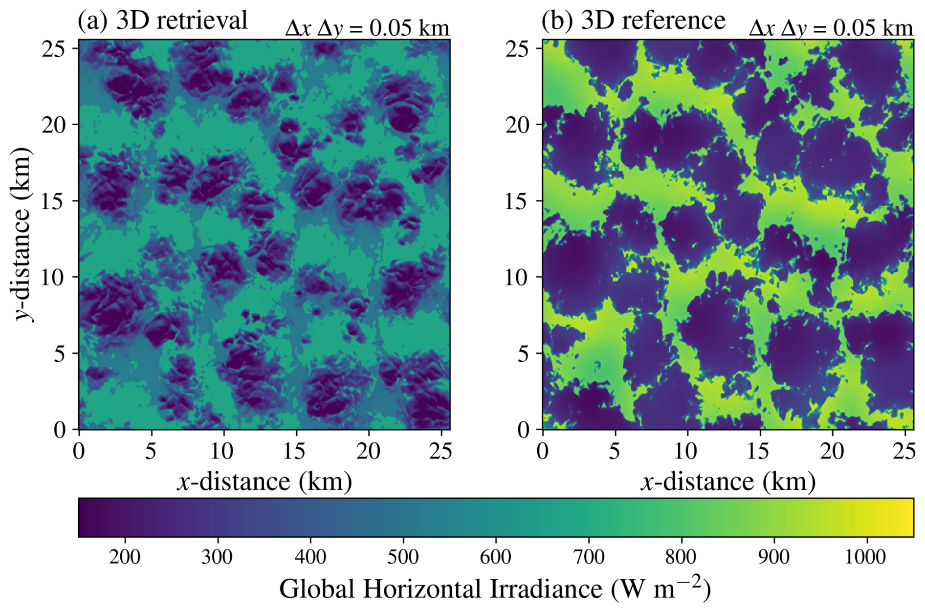
Figure 12 Spatial plots of retrieved (a) and reference (b) GHI for scene 2 at a spatial resolution of 0.05 km, for the geometry specified in Table 1.

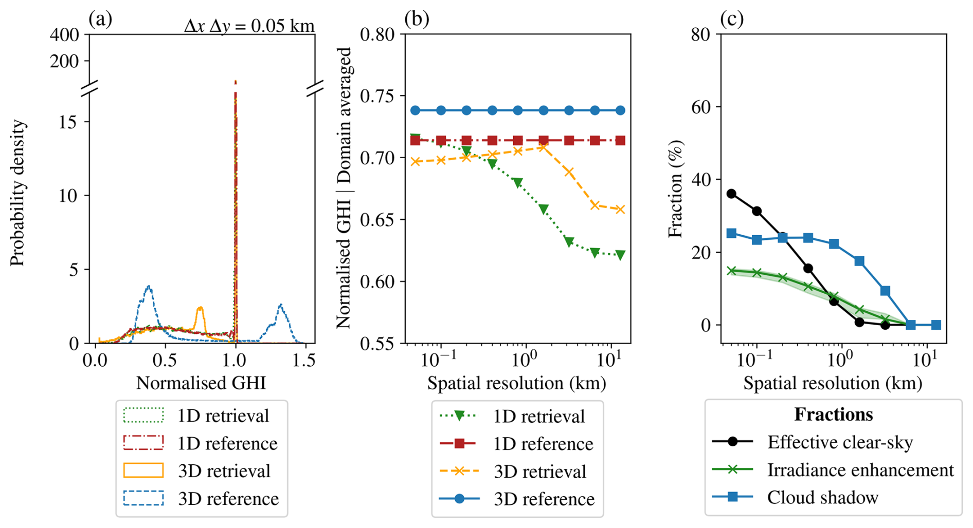
Figure 13 PDFs of GHI at 0.05 km (a) and resolution dependence of domain averaged GHI (b) for the retrieval and reference based on 1D or 3D RT, and effective clear-sky, irradiance enhancement and cloud shadow fractions, similar to Fig. 9 (c). Results are plotted for scene 2. GHI is normalised with the 3D reference clear-sky irradiance.

Overall, the distribution of 3D retrieved GHI for scene 2 follows a similar distribution as the 3D retrieved GHI from scene 1 (compare solid lines of Figs. 7e and 13a). The main difference from scene 1 is that because of the higher cloud cover, the peak in the PDF corresponding to the retrieval error due to irradiance enhancement remains more limited. Moreover, the peak occurs at slightly lower normalised GHI values. This is indicative of stronger irradiance enhancement occurring in the high cloud cover scene leading to correspondingly larger reductions in GHI. The stronger magnitude of the irradiance enhancement for scene 2 is confirmed by the 3D reference, with enhancement going up to 35 % to 40 % (compare dashed lines of Figs. 7e and 13a). Similarly to scene 1, for the 3D reference GHI a bimodal PDF is observed, but due to the larger fraction of cloudy and shaded pixels, the diffuse peak of scene 2 has a higher probability density.

In Fig. 13b, the domain averaged normalised GHI is illustrated. Generally, the trends are comparable to the corresponding low cloud cover scenario (compare Fig. 13b to Fig. 8d). Due to the higher cloud cover the absolute magnitude of domain averaged GHI is lower than for scene 1. For the 1D and 3D reference simulations, the domain averaged GHI is again preserved moving towards coarser spatial resolutions.

Next, as a result of the clear-cloudy mixing, the domain averaged GHI of the 1D retrieval reduces when the spatial resolution gets coarser (triangular-markers, Fig. 13b). Finally, just as for the scenario with low cloud cover, the 3D retrieved GHI increases towards a resolution of 1.6 km, after which it starts to decrease again (cross-markers, Fig. 13b). The difference from scenario 1 is that here the increase in GHI remains more limited, whereas the decrease in domain averaged GHI at coarser spatial resolutions is more substantial.

This can be explained again by considering the balance between the errors due to irradiance enhancement, shading, and the clear-cloudy mixing. As the initial fraction of irradiance enhanced pixels at 0.05 km is considerably lower than for scene 1 (Fig. 13c), the error due to irradiance enhancement is lower accordingly and GHI is closer to the reference. With decreasing resolution, the fraction of irradiance enhanced pixels decreases resulting in increasing domain averaged GHI. However, note that although the fraction of irradiance enhanced pixels is lower, the magnitude of the enhancements is actually larger for the high cloud cover scene (compare the solid lines from Fig. 7e with Fig. 13a). The result is a slower cancellation of the cloud enhanced pixels at decreasing spatial resolutions (Fig. 13c). Consequently, the increase in domain averaged GHI remains more limited toward coarser resolution. At a spatial resolution of 1.6 km there is a sharp decrease in domain averaged GHI. With both the irradiance enhanced and shaded pixels disappearing, clear-cloudy mixing becomes the most important error, and therefore, the domain averaged GHI is decreasing again.

From the GHI bias plots we can observe that the trends for the IPA and PPA related bias and residual bias (Fig. 14a) are comparable to those of the corresponding scenario of scene 1 (See Fig. 10d). Furthermore, also the total bias is in line with the total biases as observed for scene 1, with the smallest biases at a spatial resolution of 1.6 km. Contrary to scene 1, here, the biases at coarser spatial resolutions are larger than at the finest resolutions.

In terms of RMSE (Fig. 14b), comparing scene 1 and scene 2 shows smaller PPA and residual errors for scene 2. In contrast, for the IPA at 0.05 km spatial resolution the error is about 65 W m⁻² larger for scene 2 than for scene 1. Consequently, the IPA error remains dominant until coarser spatial resolutions. Only around a spatial resolution of 5 to 6 km does the PPA error become larger than the IPA error, while this occurs at 2 to 3 km spatial resolution for scene 1.

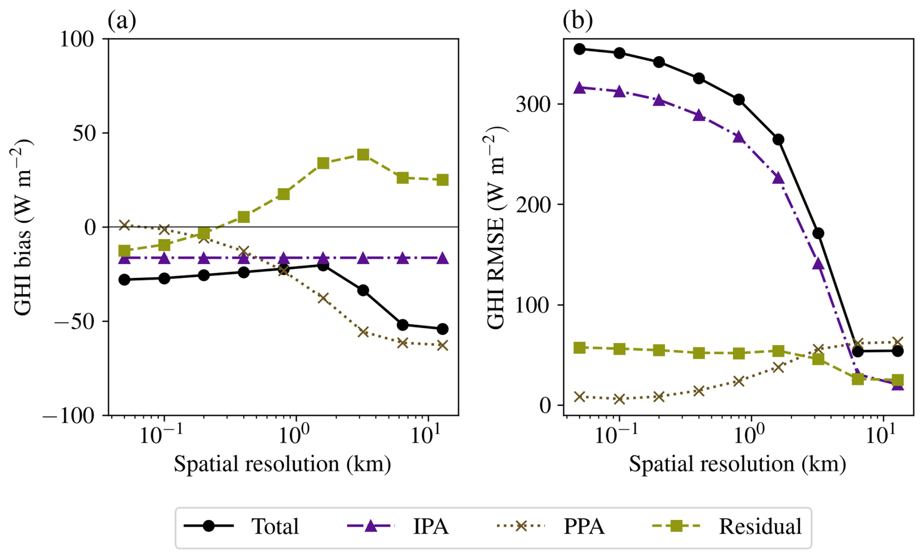
Figure 14 The total domain-averaged bias (a) and RMSE (b) as a function of spatial resolution and separated into the contributions due to the PPA, IPA and residual errors. Results are shown for Scene 2.

5 Discussion

As mentioned previously, the mixing of clear-sky and optically thin cloudy pixels with cloudy pixels with a higher τ can lead to biases in the retrieved transmittance. This section takes a closer look at these retrieval biases due to inhomogeneity. First, in Sect. 5.1, it is explained in further detail how the averaging of reflectances from adjacent clear and cloudy pixels can introduce errors in the retrieval. Then, to illustrate the implications of clear-cloudy mixing for a more complex cloud field, in Sect. 5.2, results are discussed for two final scenarios in which the retrievals are performed with slanted satellite viewing angles. The discussion section ends with an evaluation of the generalisability and remaining error sources of the conducted simulations (Sect. 5.3).

5.1 Clear and cloudy sky mixing errors

To illustrate how clear-cloudy mixing can introduce transmittance biases in the retrieval via reflectance averaging, we assume a new, highly idealised cloud field consisting of just two pixels in this section. The first pixel has a very low optical depth of 0.25, and the other pixel has a τ of either 5, 25 or 90. The satellite and solar geometry of this idealised scenario are taken directly from the DAK LUT (see Sect. 3.2) and closely match the default used in this study (Table 1).

In Fig. 15, for the chosen geometry, the relation between reflectance (solid blue curves) and optical depth as well as transmittance (dash dotted green curves) and optical depth are presented for the three optical depth contrasts between τ=0.25 and τ=5 (Fig. 15a and d), τ=25 (Fig. 15b and e) or τ=90 (Fig. 15c and f), respectively. In Fig. 15a, b, and c the narrowband TOA reflectance at 0.64 µm is plotted, while in Fig. 15d, e, and f the (hemispheric) broadband TOA albedo is shown.

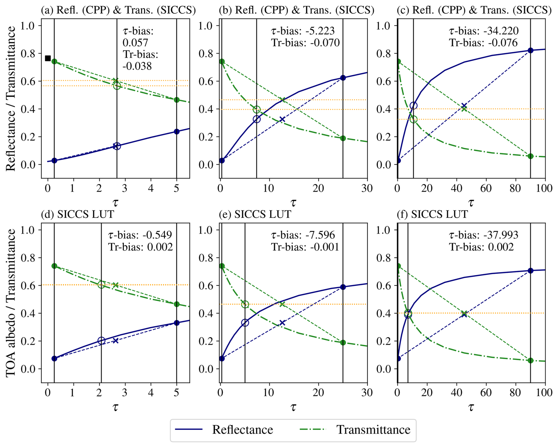
Figure 15 Illustration of how clear-cloudy mixing can introduce transmittance biases in the retrieval through the averaging of the reflectance of two pixels, one with an τ of 0.25 and the other with a τ of either 5, 25 or 90 as shown by the closed round markers. The black square in (a) represents the clear-sky transmittance. The continuous, blue lines show the 0.64 µm reflectance (a–c) or broadband TOA albedo (d–f) as a function of τ for a water cloud with r_e = 6 µm and a viewing and illumination geometry close to the default used in this study (θ₀=51°, θ=0°), simulated by DAK and taken from the the satellite retrieval LUT. The dashed-dotted, green lines show the downward transmittance of global radiation. The open round markers indicate the retrieved τ and transmittance based on the averaged reflectance of the two pixels. The crosses represent the τ and transmittance obtained by averaging the retrievals from both pixels. The difference between the horizontal dotted, yellow lines indicates the transmittance retrieval bias. The magnitudes of the τ and transmittance biases are also written in the plots.

The relation between τ and reflectance is highly nonlinear, as demonstrated by the solid, blue curves in Figure 15. As a result, coarsening of the the spatial resolution by averaging the retrieved reflectances of the two pixels (indicated by the open blue circles on the reflectance curves), leads to a substantially lower τ than would have been obtained if, instead of reflectances, the optical depth of both pixels would have been averaged (indicated by the crosses on the dashed lines between the reflectance curves).

With the optical depth determined, the next step is to derive surface irradiance. For this, the relation between τ and transmittance is used (indicated by the green dashed-dotted curves). This relation is also highly nonlinear, causing another inhomogeneity error. However, when the narrowband TOA albedo is used to retrieve τ, the relation between transmittance and optical depth is almost exactly the inverse of that between τ and TOA albedo (Figs. 15d, e, f). Hence, if broadband TOA albedo observations are used to retrieve τ and subsequently transmittance, the respective errors cancel out (see also Greuell et al., 2013): the retrieved transmittance for the combined pixel (indicated by the open green circles on the transmittance curves) is very close to the average of the retrieved transmittance for the individual pixels (indicated by the green crosses on the the dashed lines between the transmittance curves).

However, the current study does not use broadband (hemispheric) TOA albedo to derive τ but rather narrowband TOA reflectances, corresponding to measurements from satellite imagers. For these non-hemispheric observations, the relation with τ (solid lines in Figs. 15a, b, c) is slightly different from that for the broadband TOA albedo (solid lines in Figs. 15d, e, f). As a result, depending on the geometry, the τ retrieval offset is not fully compensated for by the transmittance retrieval. Indeed, the retrieved transmittance at coarse resolution (open green circles in Fig. 15a, b, c) is lower than the actual value (green crosses). Notably, if the clear-cloudy contrast grows, the magnitude of this negative transmittance bias grows accordingly, as indicated by the larger deviation between the horizontal, yellow, dotted lines in the middle and right columns.

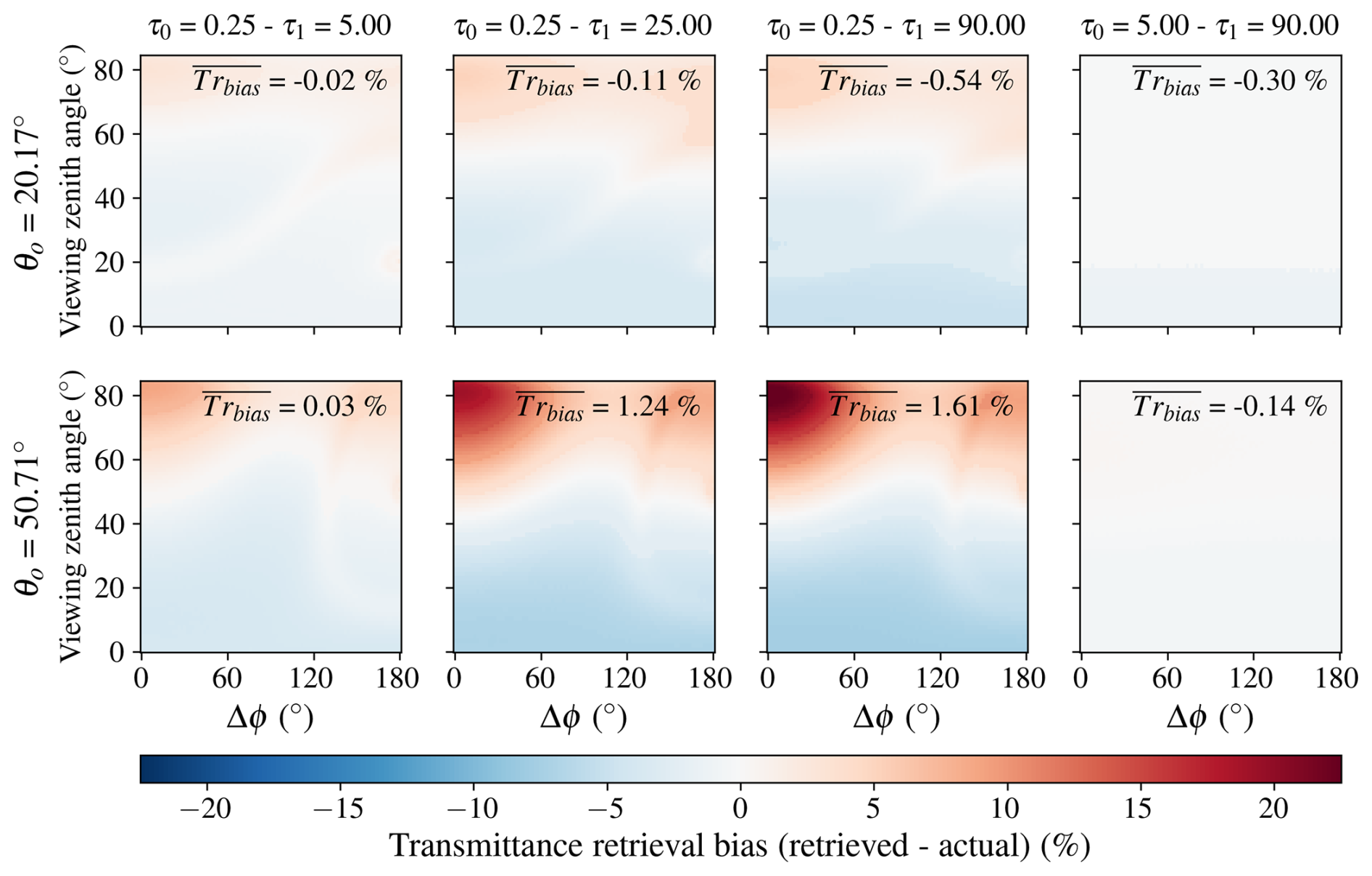
Figure 16 Transmittance retrieval bias as a function of relative azimuth angle between the Sun and the satellite (Δϕ), and viewing zenith angle. The rows show two different values of the solar zenith angle, while the columns show four combinations of low and high τ. The mean transmittance bias is indicated in each plot.

Since the hemispheric albedo leads to unbiased retrievals of transmittance (Fig. 15d, e, f), there must be specific Sun-satellite geometries for which positive transmittance biases occur as a result of the clear-cloudy mixing. In Fig. 16, the transmittance bias is shown as a function of θ and Δϕ for two values of θ₀ and four τ-contrasts. From this figure the following observations can be made. Firstly, at small satellite viewing angles, negative transmittance biases are observed, which are compensated by positive biases at high θ (above ≈ 60°). Secondly, as θ₀ grows from 20 to 50°, the overall biases, either negative or positive, increase as well, and positive transmittance biases start to occur already at lower θ. Next, as is also shown in Fig. 15, if the clear-cloudy contrast gets larger, this will generally lead to stronger transmittance biases. Moreover, the rightmost column of Fig. 16 demonstrates that clear-cloudy mixing does not lead to major transmittance biases for moderately thick to thick clouds (τ ≳ 5). In other words: the clear-cloudy mixing errors are related to retrieval at low τ. Figure 16 does not show the effect of r_e on the transmittance bias but this effect is marginal.

5.2 Viewing geometry sensitivity

With the relation between clear-cloudy mixing and viewing geometry pointed out in Sect. 5.1, here the scenarios are presented for viewing angles of 40 and 70°. By evaluating Fig. 16 for these two scenarios (also see Table 1), either limited (θ = 40°) or positive (θ = 70°), clear-cloudy mixing biases are expected.

First, for both slanted viewing angles, the PDF of the 1D retrieval is again dominated by high probability densities for the clear-sky pixels (dotted lines, Fig. 17a, d). For the retrieval based on 3D reflectances, clearer deviations are apparent compared to the default scenario. The peak in probability density corresponding to the clear-sky pixels that are incorrectly retrieved as cloudy is closer to the actual clear-sky value than for the default scenario (Compare solid lines of Fig. 17a, d to Fig. 7e). This indicates a smaller error due to irradiance enhancement as the viewing angle increases. Although the peak itself is narrower, in the scenario where θ = 70°, the peak's base is wider than in the default scenario, which we attribute to parallax.

Parallax is the shift between the actual position (from the LES data) and apparent (retrieved) position of an observed object (i.e. clouds). Until this section, all retrievals were performed for nadir viewing angles for which there is no parallax. Slanted viewing results in a shift of the projected location of the clouds in the direction away from the observer. The magnitude of parallax depends on the height of the cloud and the viewing angle (Miller et al., 2018; Wiltink et al., 2025a). Larger displacements occur for higher clouds or at larger viewing zenith angles. For the retrievals with slanted viewing angles, each pixel will have variable parallax due to variations in cloud occurrence and vertical structure. As a result, clouds that are projected onto a single pixel at nadir viewing might be projected onto multiple pixels at a higher θ, leading to smoother reflectances. If reflectances are smoothed, the retrieved cloud edges become less sharp, resulting in a smoother transition from clear to cloudy in the PDF for retrieved GHI. Due to smoothing, the retrieved cloud fraction effectively increases (not shown). Another effect of the smoothing is that both the fraction of irradiance-enhanced and cloud-shaded pixels is reduced, also reducing the retrieval error due to shading and irradiance enhancement. On the other hand, parallax does introduce an additional mismatch, as clear-sky pixels will be incorrectly classified as cloudy by the retrieval.

At a θ of 40° the change in domain-averaged GHI remains limited (triangular markers in Fig. 17b). Meanwhile, for θ = 70°, an increase in domain-averaged GHI is observed for the 1D retrieval as the resolution gets coarser (triangular markers in Fig. 17e). Both observations are as expected because with a θ of 40°, the clear-cloudy mixing bias remains limited and for θ = 70°, even a positive GHI bias is expected due to clear-cloudy mixing (see Fig. 16).

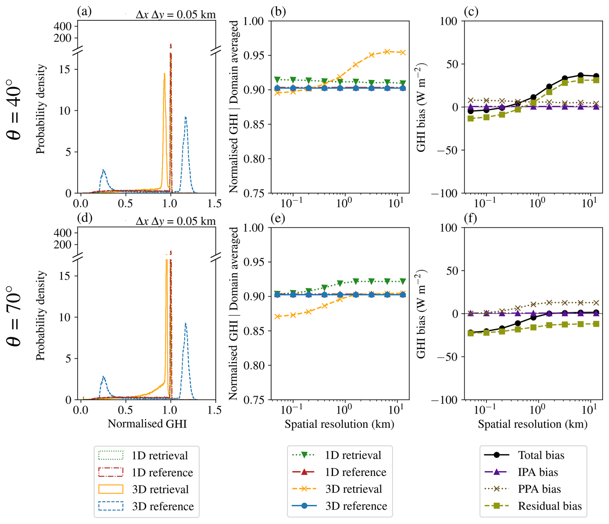
Figure 17 PDFs of GHI at 0.05 km (a, d) and resolution dependence of domain-averaged GHI (b, e) for the retrieval and reference based on 1D or 3D RT and the biases separated into the contributions due to the PPA, IPA and residual errors (c, f). The scenario is scene 1 with θ=40° (a–c) or θ=70° (d–f) and ϕ=124°. The solar position is equal to the default scenario with θ₀=51° and ϕ₀=184°.

For the retrievals based on 3D reflectances (cross markers in Fig. 17b, e), towards coarser resolutions, there is an increase in domain-averaged GHI as a result of the increase in relative importance of the retrieval error due to shading over the retrieval error due to irradiance enhancement. However, at coarser spatial resolutions, for both viewing angles, no decrease in domain-averaged GHI is observed as was the case for the default scenario of scene 1. At these coarser resolutions, the influence of irradiance enhancement and shading are limited. Moreover, for these geometries, at coarser resolutions, changes due to clear-cloudy mixing are limited as well (see 1D retrieval Fig. 17b, e), and therefore GHI remains unchanged towards even coarser resolutions.

Finally, for the biases (Fig. 17c, f), the IPA-related biases are identical to the default scenario. Since the averaged GHI of the references is constant with resolution, the PPA-related bias follows the same trend as the 1D retrieval. Next, both at a θ of 40° and a θ of 70° a positive trend in residual bias is observed if spatial resolution gets coarser. However, contrary to the scenarios with a nadir view and varying solar zenith angles, albedo, and cloud cover, for the scenario with a θ of 70°, the residual bias remains negative at all spatial resolutions. Overall, for this viewing angle, this results in a negative total bias which vanishes for spatial resolutions of 1.6 km and coarser. Interestingly, at a θ of 40° the total bias is minimal, already at a spatial resolution of 0.2 km. For most other scenarios the total bias reaches its minimum at spatial resolution between 1 and 3 km. What the scenario of θ = 40° indicates is that the observed minimal biases around 1 km, are not a general rule but heavily depend on the present geometry.

5.3 Generalisability and error sources

The current study remains limited to two variable shallow cumulus cloud fields. Results do not necessarily generalise to other cloud conditions. Likely, in more homogeneous scenes, both IPA and PPA errors will be smaller. Future studies should clarify the influence of 3D cloud-radiation interactions on retrieval accuracy in those conditions.

When generalising the presented results, not only cloud conditions should be considered. As we show in the current study, surface albedo and viewing geometry have a considerable influence on the spatial resolution at which the total bias is minimal. While the minimal total bias of the default scenario of scene 1 occurs at a spatial resolution of 1.6 km, this reduces to 0.4 (surface albedo = 0.0) or even 0.2 km (θ = 40°) in two of the sensitivity experiments.

Furthermore, in terms of RMSE, at resolutions finer than 2 to 6 km, IPA errors are the most important contributor to the overall error. Also, this balance might shift for other cloud conditions or viewing geometries. For instance, in situations with higher cloud cover and a large optical depth variability, relatively larger PPA contributions might be expected.

Although the different error components may vary strongly across cloud conditions and viewing geometries, the mechanisms describing these errors, as explained in this article, remain valid under these varying conditions, albeit with a different partitioning. Here, we focused on a single retrieval algorithm (i.e., CPP-SICCS), however, similar results would likely have been found using other 1D physics-based retrieval algorithms.

The scenarios presented in this study have been highly idealised, enabling the illustration of the first-order effect of retrieval errors due to spatial inhomogeneity and 3D radiative transfer effects. Compared to non-synthetic satellite retrievals, some deviations are expected.

For instance, for the current simulations, aerosols were excluded. Although the overall radiative effects of aerosols are much smaller than those of clouds, they still influence GHI. In the presence of aerosols, there will be a stronger extinction of irradiance from the direct beam, especially near cloud edges due to aerosol hygroscopic growth, also leading to increased scattering of radiation into cloud shadows (Gristey et al., 2022). For satellite retrievals, increased scattering would result in stronger irradiance enhancement errors in clear-sky regions. On the other hand, increased scattering towards cloud-shaded regions would reduce the errors related to shadowing.

Furthermore, the current study remains limited to a selected number of viewing geometries. These results indicate that biases depend on the viewing geometry. Therefore, the methods of the current study should be extended to other geometries to obtain a more general picture of the effect of viewing geometry on retrieval errors arising from three-dimensional cloud-radiation interactions. In terms of PPA, the transmittance biases plotted in Fig. 16 already provide a first indication of the sign and magnitude of this error across a range of viewing geometries.

6 Conclusions and outlook

In the current study, we evaluate errors in satellite retrievals of global horizontal irradiance (GHI) due to 3D cloud-radiation interactions at varying spatial resolutions. We combine retrievals of GHI based on synthetic TOA reflectances calculated from LES cloud fields with reference simulations of GHI from the same LES fields. For the forward simulations of TOA reflectance and GHI either 1D or 3D cloud-radiation interactions are considered. This yields four GHI pathways: 1D retrieval, 1D reference, 3D retrieval and 3D reference. Two highly variable shallow cumulus cloud fields with different cloud cover are considered, and the analysis is performed at resolutions ranging from 0.05 to 12.8 km. In additional sensitivity tests, the effects of solar and viewing geometry and surface albedo are studied. Since this study only presents results for two highly variable cumulus cloud fields, future studies should clarify how the presented results generalise to other cloud conditions.

From the combination of satellite retrievals and LES simulations, the retrieval error can be separated into various components. The first component is due to the plane-parallel approximation (PPA), according to which it is assumed that pixels are fully horizontally homogeneous. The magnitude of the related error therefore represents uncertainties due to unresolved sub-pixel variability. We quantify it by comparing the 1D retrieval with the 1D reference. The second component is due to the independent pixel approximation (IPA), implying that there is no radiative interaction between adjacent pixels. This makes it a measure of GHI errors due to neglect of 3D RT, which we quantify by comparing the 1D reference to the 3D reference. Finally, there is a residual error, the difference between the 1D and 3D retrieval, which measures the effect of deviations between hypothetical 1D and actual 3D TOA reflectances on 1D-retrieved GHI. In terms of bias, the above three components add up to the total retrieval error, which is the difference between the 3D retrieval and 3D reference.

The results show that in terms of the domain-averaged bias, there is to a large degree a cancellation of the errors due to the IPA. For regions with irradiance enhancement, where the GHI is above that of the clear-sky value as a result of receiving both radiation directly from the Sun in addition to diffuse radiation scattered from adjacent clouds, there is a strong positive bias. This bias is compensated by shaded regions that receive lower GHI and have a negative bias. However, locally, errors due to IPA can be substantial, which is reflected in the RMSE. In all investigated scenarios the IPA RMSE rapidly increases towards finer spatial resolutions. Depending on the scenario and its degree of 3D cloud-radiation interactions, the RMSE due to IPA becomes larger than the other components around a spatial resolution of 2 to 3 km for the low cloud cover scene and 5 to 6 km for the high cloud cover scene.

Next, the bias due to the PPA is small at the finest spatial scales but increases towards coarser spatial resolutions. The biases are introduced as a result of errors in the satellite retrieval. We explain this through an effect we call clear-cloudy mixing. Going from fine to coarse spatial resolutions, effectively, reflectances of adjacent pixels get mixed. When this happens between clear-sky or cloudy pixels with a low optical depth (τ ≲ 5) and pixels with a larger τ, transmittance biases are introduced in the retrieval. Their sign depends on the satellite viewing geometry, being generally negative, i.e. retrieved GHI is too small, for small viewing angles and positive, i.e. retrieved GHI is too large, for larger viewing angles (roughly above 60°). Furthermore, the clear-cloudy mixing error is more pronounced in case the τ-contrast is larger, and if the solar zenith angle is larger.

Finally, the residual bias is mainly characterised by two counteracting errors. The first is the retrieval error due to irradiance enhancement. In the simulation of synthetic TOA reflectances, based on 3D RT, irradiance enhancements are resolved. However, because the satellite retrieval of GHI assumes an IPA atmosphere, reflectances from irradiance enhanced pixels tend to be interpreted as cloudy. Therefore, instead of retrieving an increase in GHI for irradiance enhanced pixels, incorrectly a decreased GHI is retrieved for those pixels. The counteracting error is the retrieval error due to shading. In shaded regions reflectances are below that of the clear-sky threshold. Therefore, shaded pixels are retrieved as clear-sky and incorrectly receive clear-sky GHI instead of very low GHI values. Because in shaded regions the reflectance is often well below the clear-sky threshold, the errors due to shading can be maintained even at coarser resolutions whereas the error due to irradiance enhancements decreases already at finer spatial resolutions. In the end the magnitude of the residual bias is mainly a result of the balancing of these two counteracting errors in addition to the effect of clear-cloudy mixing.

For most simulations, when the separate bias contributions are added up, the smallest total biases are found at a spatial resolution of around 1 to 3 km, which is in line with findings from previous studies. However, this does not seem to be a general rule as the sensitivity studies show a strong dependence on surface albedo and satellite and solar geometry. For example, at a viewing zenith angle of 40°, total biases are minimal at a spatial resolution of 0.2 km.

It is well known that 3D cloud-radiation interactions lead to retrieval errors especially towards finer spatial resolutions. However, how these retrieval errors in cloud properties translate to retrieval errors of GHI has not received much attention until this study. We highlight that at finer spatial resolutions current GHI retrieval algorithms assuming the IPA prove to be insufficient to accurately resolve heterogeneous cloud conditions. This is supported by our previous work (Wiltink et al., 2025a) where we evaluated retrieved GHI based on MSG SEVIRI observations at standard (3 × 3 km) and an improved spatial resolution (1× 1 km) against ground-based observations. Without additional geolocation corrections performed, on average, GHI is more accurately retrieved at coarser spatial resolution. Note that these findings were based on a much larger number of cloud fields than the two cumulus scenes studied here.

As 3D cloud-radiation interactions become increasingly prominent at finer spatial resolutions, there is a growing necessity to account for these effects through parametrisations, corrections, or approximations using additional information. It is possible to improve the GHI retrieval accuracy at higher resolutions by applying empirical or geometric corrections for the position of the clouds (Wiltink et al., 2024, 2025a). However, the effects of these corrections remain unclear at further increased spatial resolutions. Furthermore, recent years have seen a rapid increase in the number of studies on machine learning based retrieval methods to correct for 3D radiative biases in cloud properties (e.g. Okamura et al., 2017; Masuda et al., 2019; Nataraja et al., 2022; Loveridge et al., 2025). Although these studies have shown proof-of-concept at this stage, they have not yet been widely adopted for operational use.

All in all, with the spatial resolution of the current generation of geostationary satellites going down to scales of 500 m, 3D cloud-radiation effects can limit the retrieval accuracy at these scales. Current GHI retrieval algorithms are almost exclusively 1D. To benefit from the improvements in spatial resolution, this work emphasises the need for 3D RT parametrisations and corrections for satellite-based GHI retrievals.