Long-term ozone formation sensitivity in China: spatiotemporal evolution and machine learning attribution

Accurate diagnosis of ozone (O₃) formation sensitivity (OFS) is essential for designing effective precursor-control strategies, yet long-term, observation-based, and interpretable national-scale assessments remain limited. Here, we combined OMI satellite observations of tropospheric nitrogen dioxide (NO₂) and formaldehyde (HCHO) with ground-based O₃ measurements to derive region-specific FNR (HCHO $/$ NO₂) threshold ranges from the relationship between FNR and O₃ exceedance probability. Based on these thresholds, we characterized the spatiotemporal evolution of OFS across China during the warm season (April–September) from 2005 to 2023 and coupled Random Forest (RF) with SHapley Additive exPlanations (SHAP) to quantify contributions from emission-related and meteorological factors. The results reveal a clear phase reversal in OFS over China. From 2005 to 2012, the national area fraction of nitrogen oxides (NO_x)-limited regimes decreased by 7.9 %, while transitional and volatile organic compound (VOC)-limited regimes increased by 5.6 % and 2.3 %, respectively. After 2013, this pattern reversed, and by 2023 NO_x-limited regimes expanded to 76.5 % of the polluted area, whereas VOC-limited regimes accounted for only 2.8 %. Regionally, after 2013, both Beijing–Tianjin–Hebei (BTH) and Fenwei Plain (FWP) exhibited transitions between transitional and NO_x-limited regimes, while the Yangtze River Delta (YRD) showed a shift toward NO_x-limited regimes. Sichuan Basin (SCB) remained predominantly transitional, and Pearl River Delta (PRD) also shifted toward NO_x-limited regimes. SHAP analysis shows emission-related variables contributed 50.1 %–69.4 % of total importance, exceeding meteorological factors, which increased after 2013. Overall, OFS evolution is primarily associated with emission changes but increasingly modulated by meteorological conditions under cleaner conditions.

1 Introduction

Over the past decade, China has enacted a series of unprecedented clean air policies, most notably the “Air Pollution Prevention and Control Action Plan (2013–2017)” (Chinese State Council, 2013) and the “Three-Year Action Plan for Winning the Blue Sky Defense Battle (2018–2020)” (Chinese State Council, 2018). These coordinated efforts have successfully driven substantial declines in fine particulate matter (PM_2.5), yielding a stagewise improvement in national air quality (Geng et al., 2024; Liu et al., 2024). However, surface ozone (O₃) levels have concurrently risen across major urban clusters (Li et al., 2020; Wang et al., 2022; Wei et al., 2022). This upward trend has established O₃ as the primary obstacle to further air quality gains in the post-PM_2.5 era, making China one of the regions most severely affected by O₃ pollution globally (Lu et al., 2018). Persistent elevations in O₃ concentrations are particularly evident in Beijing–Tianjin–Hebei (BTH), the Yangtze River Delta (YRD), the Pearl River Delta (PRD), the Fenwei Plain (FWP), and the Sichuan Basin (SCB) (Chen et al., 2021; Guan et al., 2021; Deng et al., 2022; Hu et al., 2024), posing documented risks to public health and ecosystem productivity (Lin et al., 2018; Liang et al., 2024a; Hua et al., 2025).

The complexity of O₃ mitigation stems from its nature as a secondary pollutant, formed through nonlinear photochemical reactions involving nitrogen oxides (NO_x = NO + NO₂) and volatile organic compounds (VOCs) (Seinfeld and Pandis, 2016). This nonlinearity implies that O₃ responses to precursor reductions vary significantly across different chemical regimes and meteorological conditions. O₃ formation sensitivity (OFS) is thus typically classified into NO_x-limited, VOC-limited, and transitional regimes (Kleinman, 1994; Sillman, 1999; Martin et al., 2004; Duncan et al., 2010; Schroeder et al., 2017). Consequently, a reliable and regionally appropriate classification of OFS regimes, together with a clear attribution of their controlling factors, is essential for developing effective, region-specific multi-pollutant control strategies.

Methods for diagnosing OFS have evolved into two primary categories: model-based and observation-based approaches (Liu and Shi, 2021). Model-based approaches mainly include source tagging techniques and sensitivity experiments within chemical transport models. Source tagging techniques determine O₃ formation regimes by tracking the contributions of precursor species, such as NO_x and VOCs, in air quality models. For instance, Wu et al. (2022) applied the Community Multiscale Air Quality (CMAQ) model coupled with the O₃ Source Apportionment Technology (OSAT) and showed that OFS in the PRD region varied substantially under different meteorological conditions. Sensitivity experiments, by contrast, estimate O₃ response to precursor emission perturbations using models such as WRF-Chem and GEOS-Chem. Using an Observation-Based Model (OBM) coupled with the WRF-CMAQ model, Zhang et al. (2024c) demonstrated dynamic shifts in northeastern China from VOC-limited or transitional regimes to NO_x-limited regimes as pollution intensifies. Although these approaches provide valuable process-level insight, they are computationally demanding and depend strongly on model performance, which limits their broad applications, especially for long-term and large-scale assessments.

Against this background, observation-based photochemical indicators provide a simpler and more efficient alternative for OFS diagnosis and regional mapping. These methods infer O₃ formation regimes from the ratios of chemically relevant species. Milford et al. (1994) initially proposed total reactive nitrogen (NO_y = NO_x + nitric acid [HNO₃] + peroxyacetyl nitrates + alkyl nitrates) as a diagnostic indicator, which was subsequently extended to indicators such as hydrogen peroxide (H₂O₂) $/$ HNO₃, O₃ $/$ NO_x, and formaldehyde (HCHO) $/$ NO_y ratios (Sillman, 1995; Tonnesen and Dennis, 2000). Among these, the satellite-based ratio of HCHO to nitrogen dioxide (NO₂), commonly referred to as FNR, has received increasing attention because of its broad spatial coverage, continuous temporal record, and strong regional representativeness (Chen et al., 2023; Li et al., 2024; Vazquez Santiago et al., 2024).

A key issue in applying FNR is the determination of appropriate threshold values for OFS classification. Duncan et al. (2010) proposed a threshold range for the United States using air quality models, a photochemical box model, and OMI-derived HCHO and NO₂ data. This range has since been widely adopted in OFS studies in China (Jin and Holloway, 2015; Itahashi et al., 2022). However, later studies showed that FNR thresholds are not universal. Schroeder et al. (2017) pointed out that regional differences, stratospheric contributions, and satellite retrieval uncertainties can all affect threshold values. Zhang et al. (2024b) further reported that FNR thresholds can also vary across time scales. These findings suggest that the commonly used fixed range of [1,2] may not be suitable for China, where precursor emissions, atmospheric environments, and meteorological conditions vary substantially across regions. Applying a uniform threshold may therefore introduce biases in OFS diagnosis.

Given these limitations, increasing efforts have been made to derive regionally appropriate FNR thresholds by combining satellite HCHO $/$ NO₂ observations with surface O₃ measurements in different parts of China (Song et al., 2023; Chen et al., 2024; Li et al., 2024). For example, Ren et al. (2022) analyzed data from April to September during 2019–2021 and found that the national-scale FNR threshold was around [2.2,3.2], whereas regional thresholds ranged from about [1.2,3.2] to [3.2,4.3]. This large range highlights substantial regional heterogeneity in OFS. Building on these studies, a more systematic evaluation of FNR thresholds across China's major city clusters is still needed to provide more reliable region-specific criteria for OFS diagnosis.

Beyond threshold determination, understanding the long-term evolution of OFS and its influencing factors is equally important. Previous studies have shown that OFS in many parts of China has shifted over the past two decades from VOC-limited regimes toward NO_x-limited or transitional regimes (Du et al., 2022; Itahashi et al., 2022; Johnson et al., 2024). This shift reflects not only changes in precursor emissions, but also the influence of meteorological variability and climate change (Zhan et al., 2022; Badia et al., 2023). Under continued climate warming, more frequent heat extremes and enhanced shortwave radiation may further alter the spatial patterns and long-term evolution of OFS (Vazquez Santiago et al., 2024). However, an understanding of how emissions and meteorology reshape OFS remains limited, particularly at the national scale and over multi-decadal periods.

To address these gaps, this study combines OMI satellite observations of tropospheric NO₂ and HCHO from 2005 to 2023 to characterize the spatiotemporal evolution of O₃ precursors and OFS across China during the warm season (April–September), with explicit comparison of the periods before and after major air quality policies (2005–2012 vs. 2013–2023). Rather than proposing a fundamentally new OFS diagnostic framework, we derive region-specific FNR threshold ranges for different regions of China based on satellite observations and surface O₃ data and use these thresholds to classify OFS regimes. We further couple a Random Forest (RF) model with SHapley Additive exPlanations (SHAP) to statistically characterize how meteorological and emission-related factors are associated with the occurrence and long-term evolution of the FNR-derived OFS states. In this framework, OFS is diagnosed using the satellite-based FNR indicator, whereas the machine learning analysis is used for driver attribution rather than to diagnose OFS directly. This framework provides a more regionally appropriate basis for OFS classification in China and offers an interpretable perspective on the relative roles of emissions and meteorology in OFS evolution.

2 Data and methods

2.1 Study area and data sources

2.1.1 Study area

This study focuses on mainland China and five major urban clusters with severe O₃ pollution, namely the Beijing–Tianjin–Hebei (BTH) region, the Yangtze River Delta (YRD), the Fenwei Plain (FWP), the Pearl River Delta (PRD), and the Sichuan Basin (SCB) (Fig. 1). These regions were selected because they have persistently high O₃ levels and are widely recognized as major O₃ pollution hotspots in China (Ozone Pollution Control Committee of Chinese Society of Environmental Sciences, 2024). They also represent distinct combinations of emission characteristics, meteorological conditions, and topographic settings, making them suitable for examining the regional heterogeneity of OFS (Wang et al., 2017; Zhang et al., 2025b).

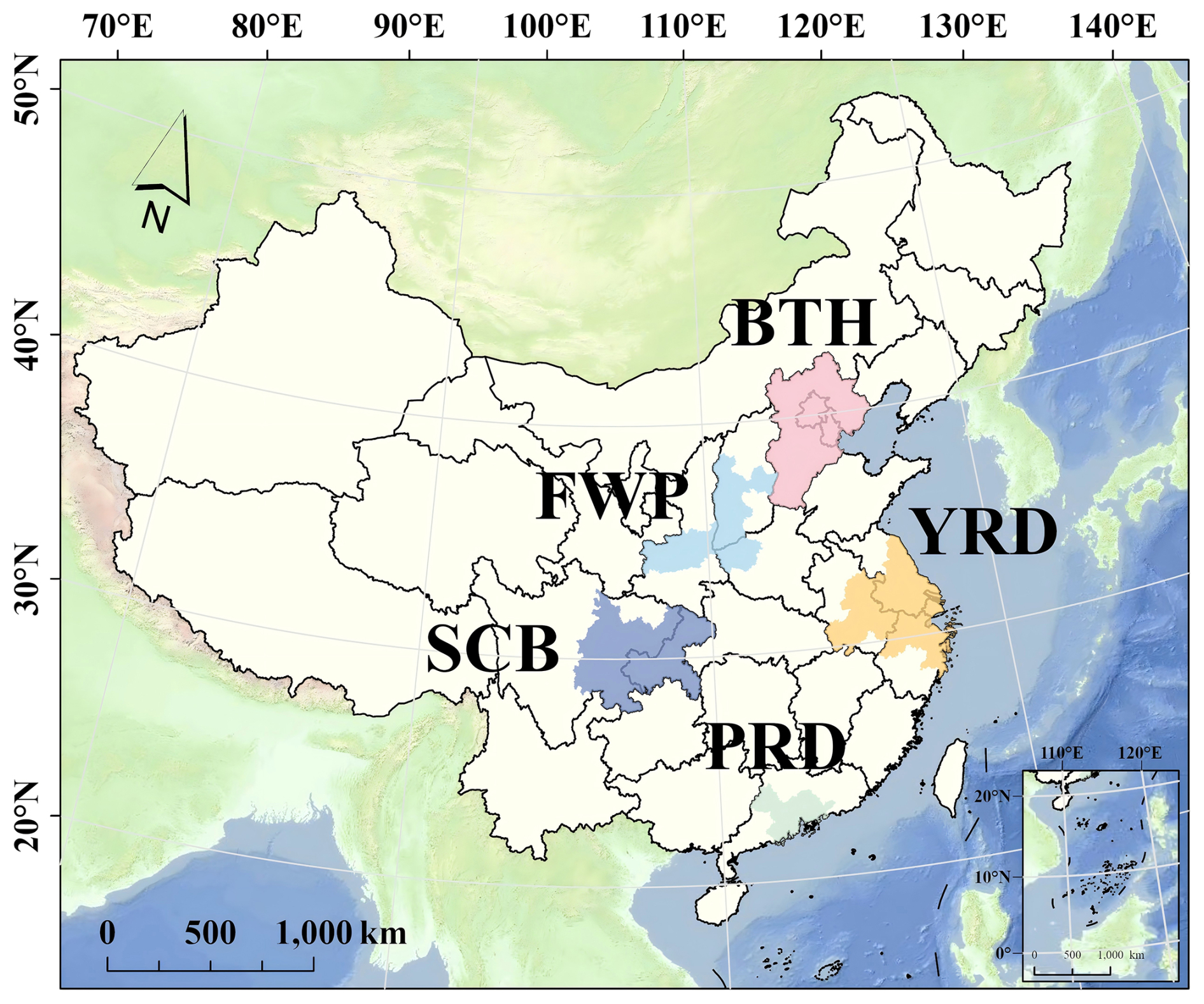
Figure 1 Study domain and five key city clusters: Beijing–Tianjin–Hebei (BTH), Fenwei Plain (FWP), Yangtze River Delta (YRD), Sichuan Basin (SCB), and Pearl River Delta (PRD).

2.1.2 Satellite data

NO_x has a short lifetime in the boundary layer, and NO is rapidly converted to NO₂. Therefore, the NO₂ column is commonly used as a proxy for ambient NO_x levels (Duncan et al., 2010). HCHO is a major intermediate product of VOCs oxidation, with a relatively short lifetime and a dominant distribution in the troposphere, making its total column abundance a useful indicator of tropospheric VOCs (Duncan et al., 2010).

In this study, daily NO₂ and HCHO column data from 2005 to 2023 were obtained from the Ozone Monitoring Instrument (OMI) onboard Aura satellite, available from the National Aeronautics and Space Administration (NASA) Goddard Earth Sciences Data and Information Services Center (https://disc.gsfc.nasa.gov/, last access: 6 September 2025). Launched in 2004, OMI provides daily near-global observations with a minimum spatial resolution of approximately 13 × 24 km and an overpass time of about 13:45 local time (LT) (Levelt et al., 2006).

Tropospheric NO₂ data were taken from the OMNO2d Level-3 product, which provides daily tropospheric NO₂ columns at a spatial resolution of 0.25° × 0.25° in units of molec. cm⁻², and retains only pixels with cloud fraction below 30 % (Krotkov et al., 2019). HCHO data were obtained from the Level-3 OMHCHOd product with a spatial resolution of 0.1° × 0.1° (Chance, 2019). This product is generated based on the Level-2 OMHCHO retrievals after applying quality control filters to exclude pixels with cloud fractions > 0.3, solar zenith angles > 70°, or those affected by the OMI row anomaly. The HCHO columns were retrieved using the Smithsonian Astrophysical Observatory (SAO) algorithm, with typical values ranging from 4 × 10¹⁵ to 4 × 10¹⁶ molec. cm⁻² and with a detection limit of approximately 1.0 × 10¹⁶ molec. cm⁻² (González Abad et al., 2015). Following Zhu et al. (2017), only values between −0.5 × 10¹⁶ and 1.0 × 10¹⁷ molec. cm⁻² were retained, while values outside this range were treated as outliers and removed. To reduce random noise, a 3 × 3 moving average based on the eight-neighborhood was applied to the HCHO fields. The smoothed HCHO data were then resampled to a 0.25° × 0.25° grid using bilinear interpolation to match the NO₂ product, following an approach similar to that of Koukouli et al. (2016) for sulfur dioxide (SO₂) data.

2.1.3 Meteorological data

Meteorological data for 2005–2023 were obtained from the ERA5 reanalysis dataset produced by the European Centre for Medium-Range Weather Forecasts (ECMWF) (Hersbach et al., 2020; https://cds.climate.copernicus.eu/, last access: 14 September 2025). ERA5 provides monthly data at a spatial resolution of 0.25° × 0.25°, which were further regridded to match the OMI NO₂ grid. The meteorological variables used in this study include 2 m temperature (T), relative humidity at 1000 hPa (RH), surface solar radiation downwards (SSRD), 10 m wind speed (WS), surface pressure (SP), and boundary layer height (BLH) (Weng et al., 2022).

2.1.4 Anthropogenic emission data

Anthropogenic emission data for 2005–2023 were obtained from the Multi-resolution Emission Inventory for China (MEIC, http://www.meicmodel.org/, last access: 14 September 2025) developed by Tsinghua University, covering five sectors: power, industry, residential, transportation, and agriculture (Li et al., 2017). MEIC provides ten major species: SO₂, NO_x, carbon monoxide (CO), ammonia (NH₃), carbon dioxide (CO₂), non-methane volatile organic compounds (NMVOCs), fine particulate matter (PM_2.5), inhalable particles (PM₁₀), black carbon (BC), and organic carbon (OC) (Zheng et al., 2018; Geng et al., 2024). Following Zhang et al. (2024a) and related work linking emissions to O₃ variability via machine learning (ML), we selected monthly emissions of NO_x, NMVOCs, CO, and PM_2.5 as key predictors for diagnosing OFS. All emission data were resampled to 0.25° × 0.25° to match the grid of satellite NO₂ data, ensuring spatial consistency across datasets.

2.1.5 Surface observation data

Surface O₃ concentration data for 2015–2023 (µg m⁻³) used in this study were obtained from China's national air quality monitoring network. Since 2015, this network has expanded to include more than 330 cities and over 1400 monitoring stations nationwide. The data were collected from the National Real-time Urban Air Quality Publishing Platform provided by the China National Environmental Monitoring Centre (https://air.cnemc.cn:18007/, last access: 20 January 2026).

2.2 Methodology

2.2.1 Diagnosis of OFS and derivation of FNR threshold ranges

OFS was diagnosed using the satellite-based HCHO $/$ NO₂ ratio (FNR), defined as:

$$\begin{array}{}\text{(1)}& \text{FNR}={\displaystyle \frac{\left[\mathrm{HCHO}\right]}{\left[{\mathrm{NO}}_{\mathrm{2}}\right]}},\end{array}$$

where [HCHO] and [NO₂] represent the tropospheric column densities of HCHO and NO₂, respectively. Because the two quantities have the same units, FNR is dimensionless.

OFS regimes were then identified according to the corresponding FNR threshold ranges. The threshold ranges were determined mainly following the method of Jin et al. (2020). In this study, region-specific FNR thresholds across China were derived by combining OMI satellite observations with surface O₃ measurements. This approach is also consistent with previous studies that derived threshold ranges from fitted O₃–FNR relationships (Wang et al., 2021; Ren et al., 2022; Chen et al., 2024). In practice, the transition of OFS from VOC-limited to NO_x-limited regimes is gradual rather than abrupt. This transition can be influenced by multiple factors, including topography, meteorological conditions, and the spatial resolution of satellite observations (Jin et al., 2020). Because these influencing factors vary across China, the corresponding FNR threshold ranges are also expected to differ among regions. For this reason, OFS regimes were identified using region-specific FNR threshold ranges. China was divided into six regions, including five major urban clusters with severe O₃ pollution, namely BTH, FWP, YRD, SCB, and PRD, and one additional category comprising all remaining areas, referred to as other regions of China (ORC) (Lu et al., 2018). These six regions were used as the basic units for deriving region-specific FNR threshold ranges, which were then applied to identify OFS regimes in each region.

Because O₃ pollution in China occurs mainly during the warm season (April–September) (Lu et al., 2020b), the analysis was restricted to April–September in 2015–2023. To match the OMI overpass time, surface O₃ concentrations at 13:00 and 14:00 LT were averaged for each site and day. The resulting daily O₃ concentrations were then collocated with OMI FNR values at the corresponding grid cells. For each site, the high-O₃ probability was then defined as the fraction of days during the study period on which the 13:00–14:00 mean O₃ concentration exceeded 160 µg m⁻³. The resulting paired samples were subsequently pooled within each region for threshold derivation.

To focus on polluted conditions, samples with NO₂ vertical column densities below 1.5 × 10¹⁵ molec. cm⁻² were excluded, following previous studies (Jin et al., 2020; Wang et al., 2021). In addition, high-end outliers (5 % or 10 %, depending on the region) were removed prior to fitting to reduce the influence of extreme values (Chen et al., 2024). After quality control, paired high-O₃ probability and FNR samples in each region were grouped into 100 bins according to FNR and a cubic polynomial was fitted to the binned relationship between high-O₃ probability and FNR. The FNR interval corresponding to fitted high-O₃ probability values above the 90th percentile was then defined as the threshold range for that region (Jin et al., 2020).

2.2.2 Trend analysis and statistical testing methods

To quantify the spatiotemporal trends of NO₂ and HCHO columns during the warm season (April–September) from 2005 to 2023, we applied the nonparametric Mann–Kendall (MK) test for trend significance (Hirsch et al., 1982) and the Sen's slope for trend magnitude (Sen, 1968). The MK statistics are computed from all pairwise differences in a time series:

$$\begin{array}{}\text{(2)}& S={\sum }_{i=\mathrm{1}}^{n-\mathrm{1}}{\sum }_{j=i+\mathrm{1}}^n\text{sgn}\left(x_j-x_i\right),\end{array}$$

where n is the number of observations, x_i and x_j are values at times i and j, respectively (j > i), and sgn(⋅) is the sign function that quantifies the direction of change between two observations: it returns 1 when a later value (x_j) is greater than an earlier one (x_i), −1 when it is less, and 0 when they are equal. A positive (negative) S indicates an increasing (decreasing) trend. Statistical significance is assessed using the standardized test statistic Z:

$$\begin{array}{}\text{(3)}& Z=\left\{\begin{array}{ll}\frac{S-\mathrm{1}}{\sqrt{\text{Var}\left(S\right)}}& S>\mathrm{0}\\ \mathrm{0}& S=\mathrm{0}\\ \frac{S+\mathrm{1}}{\sqrt{\text{Var}\left(S\right)}}& S<\mathrm{0}\end{array}\right.,\end{array}$$

where Var(S) represents the variance of the statistic S. When $\left|Z\right|$ ≥ 1.96, the trend is considered statistically significant at the 95 % confidence level (p < 0.05).

Trend magnitude is estimated by the Sen's slope β, defined as the median of all pairwise slopes:

$$\begin{array}{}\text{(4)}& \mathit{\beta }=\text{Median}\left({\displaystyle \frac{x_j-x_i}{t_j-t_i}}\right),\end{array}$$

where t_i and t_j represent the time points of observations i and j, respectively. This MK–Sen framework is distribution-free and robust to outliers, making it well suited to satellite-derived time series.

To further identify structural shifts in the long-term evolution of O₃ precursors and OFS, and to provide an objective basis for subsequent phase-based analyses, we applied the Pettitt test to the annual time series of NO₂, HCHO, and FNR in each region. The Pettitt test is a non-parametric method for detecting a single abrupt change point in a time series and does not require the data to follow a normal distribution (Pettitt, 1979). It has been widely used in environmental studies to detect statistically significant shifts in long-term observations (Baruah et al., 2022). The test statistic U_t,n is defined as:

$$\begin{array}{}\text{(5)}& U_{t,n}={\sum }_{i=\mathrm{1}}^t{\sum }_{i=t+\mathrm{1}}^n\text{sgn}\left(x_j-x_i\right)\left(t=\mathrm{1},\mathrm{2},\mathrm{\dots },n\right),\end{array}$$

where x_i and x_j are the values of the time series, and sgn(⋅) denotes the sign function. The change point is identified as the time corresponding to the maximum absolute value of U_t,n, and its significance is evaluated as:

$$\begin{array}{}\text{(6)}& p=\mathrm{2}\exp \left(-{\displaystyle \frac{\mathrm{6}{k}_t^{\mathrm{2}}}{n^{\mathrm{3}}+n^{\mathrm{2}}}}\right),\end{array}$$

where k_t = ${max}_{\mathrm{1}\le t<n}\left|U_{t,n}\right|$. A p value below 0.05 was considered statistically significant.

In this study, the Pettitt test was applied to the annual warm-season (April–September) series of NO₂, HCHO, and FNR for each region during 2005–2023. For each variable, the year corresponding to the maximum absolute test statistic was taken as the detected change point. Because the Pettitt test identifies only one abrupt change point, it may not fully capture series with multiple shifts or several equally strong candidates (Zhang and Song, 2015). Therefore, the detected change points were interpreted together with the temporal evolution of each variable and the broader policy context.

2.2.3 Machine learning model

Random Forest (RF) is an ensemble machine learning (ML) algorithm based on multiple decision trees and is widely used for classification and regression (Breiman, 2001). It implements Bootstrap aggregation (bagging): each tree is trained on a bootstrap replica of the training data with feature randomness at each split, and predictions are combined by majority vote for classification or arithmetic averaging for regression to improve generalization and robustness (Breiman, 1996).

Departing from most studies that regress O₃ concentrations on candidate factors (Luo et al., 2024; Yao et al., 2024), we frame the problem as classification to identify the key factors distinguishing OFS regimes. In this setting, the RF seeks to minimize overall misclassification. Given an input and an ensemble of trees, the predicted class is the plurality vote:

$$\begin{array}{}\text{(7)}& \widehat{y}={\text{argmax}}_k{\sum }_{t=\mathrm{1}}^{T}I\left(h_t\left(x\right)=k\right),\end{array}$$

where I(⋅) is the indicator function, equal to 1 if the tth tree assigns the sample to class k, and 0 otherwise.

This study constructs RF classification models for five city clusters, including BTH, FWP, YRD, SCB, and PRD, to characterize the relationships between OFS, defined based on the FNR classification, and multiple environmental factors. Predictor variables included anthropogenic emissions, namely NO_x, NMVOCs, CO, and PM_2.5, as well as meteorological parameters, including T, RH, SSRD, WS, SP, and BLH. It should be noted that, although OFS is diagnosed here using the FNR indicator, the spatiotemporal distribution of FNR-derived OFS states is jointly shaped by precursor emissions, chemical transformation, transport, dilution, and boundary-layer mixing (Bai et al., 2018; Chen et al., 2020; Liu and Shi, 2021). Meteorological conditions therefore do not enter the OFS definition directly but can influence the probability of different OFS states by modulating the underlying precursor environment. Based on this rationale, we treat the diagnosed OFS regimes as response classes and use RF to statistically map their relationships with meteorological and emission-related predictors.

Model training and evaluation were based on annual mean gridded data for the warm seasons (April–September) from 2005 to 2023. Because the primary aim of this study was not to predict OFS in future years, but to characterize the relationships between OFS regimes and their environmental factors over the full study period, a year-wise stratified random sampling strategy was adopted. In studies aimed at predicting future years, a common practice is to train the model on earlier-period data and validate it on later-period data in order to assess temporal extrapolation skill (Ni et al., 2024; Wang et al., 2023). Such a strategy was not adopted here because it would bias model evaluation and subsequent SHAP interpretation toward the late-period data distribution. Instead, samples from each year were randomly divided into 80 % for training and 20 % for validation (Özüpak et al., 2025), so that both subsets contained data from all years. This design preserves interannual variability associated with key periods, including major policy interventions and the COVID-19 pandemic, while maintaining comparable sample distributions across the training and validation sets. In addition, given the class imbalance in the dataset, this stratified sampling strategy helps maintain a more balanced class distribution in both subsets, thereby improving the reliability of model evaluation (Sadaiyandi et al., 2023). It also provides a more suitable basis for subsequent SHAP-based interpretation across different temporal subsets, thereby facilitating comparisons of OFS regimes before and after policy implementation.

To account for class imbalance and optimize model performance, the Synthetic Minority Over-sampling Technique (SMOTE; Fernandez et al., 2018) was applied to the training data. To reduce the structural differences of the model and facilitate consistent comparison across the five regions, a unified set of model parameters was adopted for all regional models. Although this does not eliminate differences in model baseline and data distribution across regions, it helps ensure that the regional models are constructed under a consistent modeling framework. Hyperparameter optimization was performed using GridSearchCV (Hastie et al., 2009; Ahmed et al., 2025) over combinations of candidate parameter values. Based on validation performance across all regions, a single parameter set was selected as the optimal configuration. The final model configuration consisted of 200 trees (n_estimators = 200), a maximum tree depth of 25 (max_depth = 25), and a minimum of 1 sample per leaf (min_samples_leaf = 1).

Model performance on the validation set was evaluated using multiple metrics, including precision score (PS), recall score (RS), F1-score (F1), accuracy score (AS), geometric mean score (GMS), and the Area Under the Curve of the Receiver Operating Characteristic (ROC-AUC) score (Thieu, 2024; Ahmed et al., 2025). All of these metrics range from 0 to 1, with higher values indicating better performance.

2.2.4 SHapley Additive exPlanations approach

SHapley Additive exPlanations (SHAP) is an interpretable ML framework based on cooperative game theory that explains model prediction by assigning each feature a Shapley value representing its contribution to the prediction (Lundberg and Lee, 2017). It is defined as follows:

$$\begin{array}{}\text{(8)}& \begin{array}{rl}{\mathit{\phi }}_i=& {\sum }_{\text{S}\subseteq \left\{\mathrm{1},\mathrm{\dots },n\right\}\backslash \left\{i\right\}}{\displaystyle \frac{\left|\text{S}\right|\mathrm{!}\left(n-\left|\text{S}\right|-\mathrm{1}\right)\mathrm{!}}{n\mathrm{!}}}\\ & \left[f\left(\text{S}\bigcup \left\{i\right\}\right)-f\left(\text{S}\right)\right],\end{array}\end{array}$$

where φ_i is the SHAP value of feature i, S represents the feature subset excluding feature i, f(S⋃{i}) and f(S) are the model predictions for the corresponding subsets, and $\frac{\left|\text{S}\right|\mathrm{!}\left(n-\left|\text{S}\right|-\mathrm{1}\right)\mathrm{!}}{n\mathrm{!}}$ ensures that the contributions of all feature subsets are fairly distributed.

A positive SHAP value indicates that a given feature increases the model prediction, whereas a negative SHAP value indicates that it decreases the prediction. In this study, SHAP values were calculated for the RF models in different regions to identify the key factors of OFS regimes, including NO_x-limited, transitional, and VOC-limited regimes, and to further interpret the direction and relative magnitude of their effects.

For each regional model, the mean absolute SHAP value [mean(|SHAP|)] was calculated for each feature. Because SHAP values are defined relative to the model-specific expected output and are influenced by the underlying data distribution, the absolute magnitudes of SHAP values are not directly comparable across different regional models. Therefore, to facilitate cross-region comparison, these overall mean(|SHAP|) values were further normalized to obtain the relative contribution of each variable within each regional model. It should be noted that this metric reflects the statistical contribution of individual features to model predictions rather than their direct causal effects in atmospheric physical or chemical processes.

3 Results and discussion

3.1 Spatiotemporal evolution of ozone precursors

Before examining the spatial and temporal evolution of O₃ precursors and FNR, we first assessed whether their long-term changes were characterized by structural shifts. Pettitt test results (Table S2 in the Supplement) indicate that significant change points in warm-season NO₂, HCHO, and FNR were generally clustered around 2013–2017, although the exact timing varied among variables and regions. Because these shifts broadly coincided with the implementation of the Air Pollution Prevention and Control Action Plan (2013–2017), 2013 was adopted as the common dividing year for the subsequent analyses. The following sections therefore compare the two periods 2005–2012 and 2013–2023.

Under this phase-based framework, the spatial patterns and long-term trends of tropospheric NO₂ and HCHO columns were further examined (Fig. 2). High NO₂ columns are mainly concentrated in densely populated and industrialized urban clusters, including the BTH, YRD, and PRD regions (Fig. 2a), reflecting intensive energy use and traffic emissions in eastern China (Fu et al., 2022). Among the five key regions, BTH shows the highest annual mean NO₂ column (7.41 × 10¹⁵ molec. cm⁻²), which is 2.56 times that in SCB (2.90 × 10¹⁵ molec. cm⁻²) (Fig. S1 in the Supplement). This pattern is consistent with the concentration of heavy industry (e.g., steel production) and the widespread use of coal for winter heating in northern China (Li et al., 2010; Feng et al., 2014). In terms of temporal evolution, NO₂ showed a clear phase shift around 2013. From 2005 to 2012, NO₂ increased by 31.5 % at the national scale, with the strongest growth occurring in eastern China and a maximum trend of 1.16 × 10¹⁵ molec. cm⁻² yr⁻¹. The PRD was a notable exception in which NO₂ decreased by 23.3 % during the same period, with a maximum trend of −1.21 × 10¹⁵ molec. cm⁻² yr⁻¹, likely reflecting earlier industrial restructuring and vehicle emission controls (Bian et al., 2019; Lu et al., 2020a). After the implementation of major clean air policies in 2013, NO₂ showed a widespread decline across China (Fig. 2c), with a national decrease of 27.6 % and the largest reductions occurring in eastern urban clusters. The maximum decline reached −1.37 × 10¹⁵ molec. cm⁻² yr⁻¹, indicating a clear response of NO_x to emission-control policies (Shah et al., 2020; Li et al., 2023). This shift in NO₂ is an important background for subsequent changes in OFS.

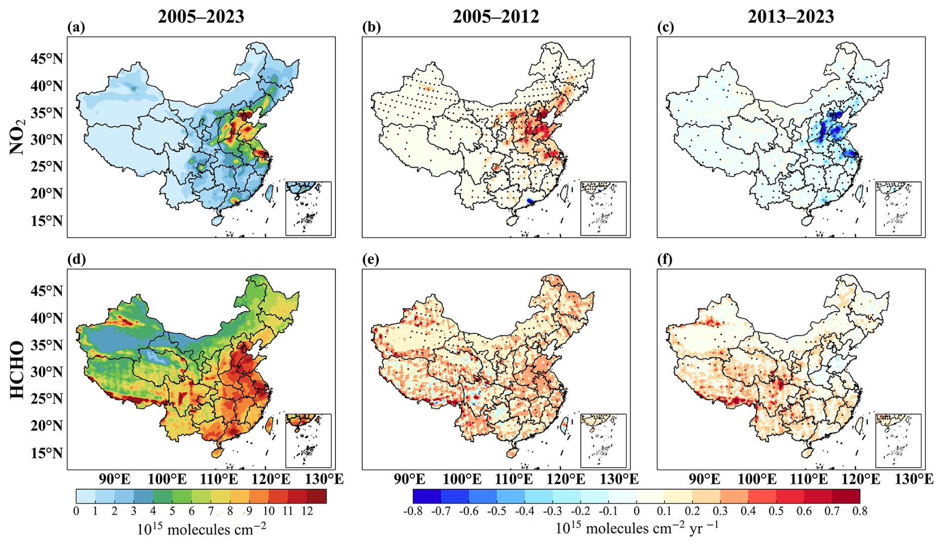
Figure 2 Spatiotemporal variations of tropospheric NO₂ and HCHO columns over China during the warm season (April–September) from 2005 to 2023. (a, d) Distribution of annual average columns for 2005–2023; spatial distributions of the Sen's slope and Mann–Kendall (MK) test results for annual means during (b, e) 2005–2012 and (c, f) 2013–2023. Black dots in panels (b), (c), (e), (f) mark grids that pass the MK significance test (p < 0.05).

Compared with NO₂, HCHO exhibits a more complex spatial distribution. Elevated HCHO columns are observed not only over the major urban clusters in eastern China, but also across parts of southwestern and western China, including Guangxi, Yunnan, western Sichuan, and southern Tibet, where the values can even exceed those over some eastern urban regions (Fig. 2d). Such high values may partly reflect enhanced HCHO production associated with strong biogenic VOCs (BVOCs) emissions under warm conditions and intense solar radiation (Zhang et al., 2025a). However, they may also be influenced by the relatively large retrieval uncertainties in western China, especially over the Qinghai–Tibet Plateau and surrounding areas, where complex terrain and surface conditions can affect satellite retrieval accuracy (Fig. S2; Xia et al., 2024). Therefore, the elevated HCHO columns in these regions likely result from a combination of real atmospheric signals and retrieval uncertainties and should be interpreted with caution. Among the five key regions, the PRD has the highest annual mean HCHO column (10.60 × 10¹⁵ molec. cm⁻²) (Fig. S1), reflecting the combined influence of strong anthropogenic emissions and substantial biogenic contributions (Xia et al., 2024).

The temporal evolution of HCHO differs markedly from that of NO₂. During 2005–2012, HCHO increased modestly at the national scale, with an average trend of 0.17 × 10¹⁵ molec. cm⁻² yr⁻¹, corresponding to an increase of 19.5 %. The most pronounced increases occurred along the urban corridor from North China to East China. From 2013 to 2023, a clear increasing trend emerged over large parts of northwestern China, and the national HCHO column increased by 20.8 %. The continued rise after 2013 may be related to two factors. First, regional warming and enhanced shortwave radiation can stimulate BVOCs emissions (Wang et al., 2024). Second, NO_x emissions declined more rapidly than anthropogenic VOCs (AVOCs) (Itahashi et al., 2022), which may have altered the photochemical environment and increased both the production efficiency and atmospheric lifetime of HCHO. The sustained increase in HCHO is also consistent with the continued rise in surface O₃ observed in China over the past decade (Wang et al., 2022).

Overall, the long-term evolution of O₃ precursors reflects the combined influence of emission-control policies and climate-related factors. NO_x declined substantially in response to anthropogenic emission reductions, whereas HCHO continued to increase in many regions, consistent with previous studies (Bauwens et al., 2022), and these HCHO changes have been primarily attributed to meteorological variability and natural emissions (Itahashi et al., 2022; Vazquez Santiago et al., 2024). This asynchronous evolution of NO₂ and HCHO provides an important precursor basis for the subsequent shifts in FNR and OFS across China.

3.2 Determination of region-specific FNR threshold ranges

To derive region-specific FNR threshold ranges, we first examined the nonlinear relationship between O₃ formation and its precursors using satellite-derived HCHO and NO₂. Figure S3 shows the distribution of high-O₃ probability in the two-dimensional HCHO–NO₂ space for the six regions. The overall pattern is similar to the O₃ contour structure reported in previous studies (Sillman, 1999), indicating that HCHO and NO₂ can reasonably serve as proxies for VOCs and NO_x, respectively, in characterizing the nonlinear response of O₃ formation. Based on this relationship, each region can be broadly divided into three OFS regimes: a NO_x-limited regime under relatively high HCHO and low NO₂ conditions, a transitional regime under relatively high levels of both HCHO and NO₂, and a VOC-limited regime under relatively low HCHO and high NO₂ conditions.

Based on the fitted high-O₃ probability-FNR relationships, region-specific threshold ranges were derived for the six regions, reflecting the gradual transition among OFS regimes. Figure 3 shows the fitted relationships for the six regions during the warm season (April–September) of 2015–2023. Clear regional differences are found in the derived FNR threshold ranges. Among the six regions, FWP shows the highest threshold range, with a central threshold of 3.42 and a range of [2.26,4.77], whereas YRD shows the lowest, with a central threshold of 1.59 and a range of [0.90,2.37]. The corresponding threshold ranges for BTH, SCB, PRD, and ORC are [1.51,3.30], [1.93,4.73], [1.66,3.70], and [1.17,3.08], respectively. In terms of fitting performance, the correlation coefficient is 0.58 in FWP and exceeds 0.60 in the other regions, reaching 0.96 in ORC, with all p values below 0.05. These results indicated that the fitted curves generally capture the variation in high-O₃ probability well. Comparison with previous studies (Table S1) further shows that FNR thresholds vary across regions, reflecting differences in atmospheric environment, precursor emissions, and local conditions (Liu and Shi, 2021).

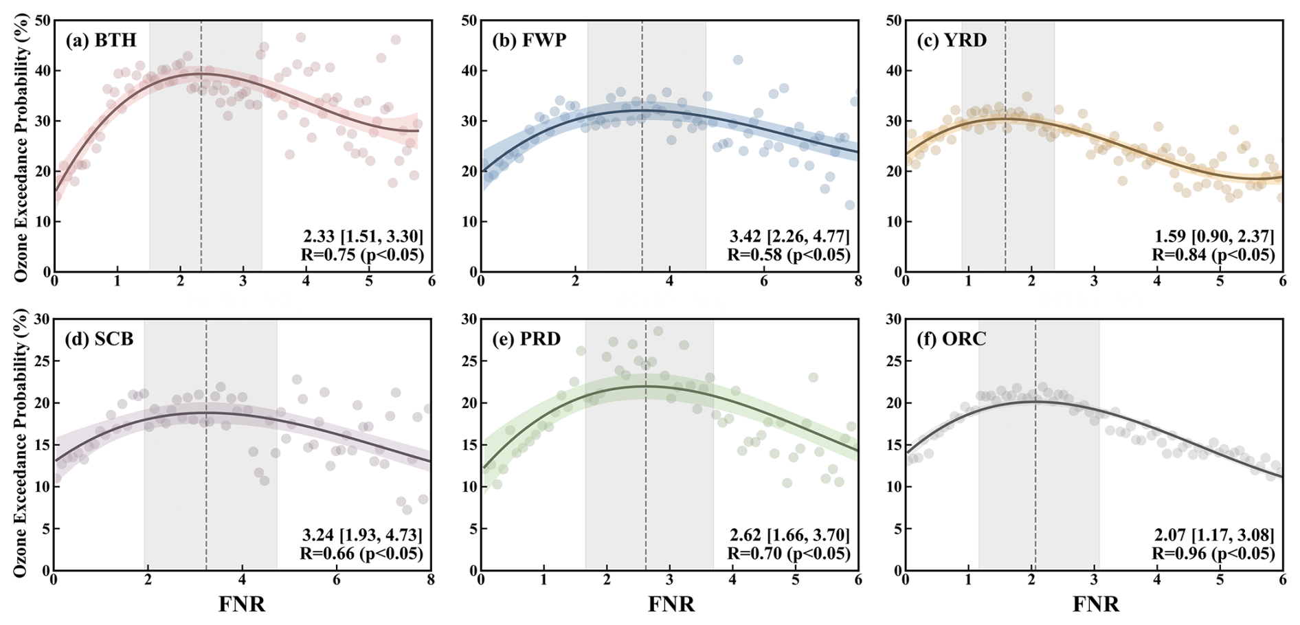
Figure 3 Relationship between daily high-O₃ probability and FNR in the six regions during the warm season (April–September) of 2015–2023. Solid lines show the fitted cubic polynomial curves, and the shaded areas indicate the 95 % confidence intervals. Vertical dashed lines mark the peak values of the fitted curves, while the gray shaded bands denote the FNR ranges corresponding to the upper 10 % of the fitted curves, which were used to define the threshold ranges.

Given these pronounced regional differences, we further assessed how threshold uncertainty affects OFS classification. Three threshold-range scenarios were designed. Specifically, Scenario 1 (S1) used the threshold ranges derived in this study for the warm season of 2015–2023, Scenario 2 (S2) adopted the minimum–maximum threshold ranges reported in previous studies, and Scenario 3 (S3) used threshold ranges calculated from the average of the corresponding maximum and minimum values. The threshold ranges for the six regions under S1–S3 scenarios are listed in Table S1. These three scenarios were then used to evaluate the sensitivity of OFS classification to different FNR threshold selections in the five major city clusters during the warm season over 2005–2023 (Fig. S4).

The results show that OFS classification is strongly affected by threshold choice, although the magnitude of this effect varies markedly across regions. Among the five regions, FWP shows the largest sensitivity to threshold variation, with changes ranging from −53.8 % to 51.6 % and an average value of about 22.0 %. SCB also exhibits substantial sensitivity, with corresponding changes of −48.8 % to 52.0 %. In contrast, PRD is relatively less sensitive, with changes ranging from −36.3 % to 21.1 % and an average value of about 17.0 %. BTH and YRD show intermediate responses, with ranges of −31.0 % to 37.2 % and −31.5 % to 31.5 %, respectively. These results indicate that the uncertainty introduced by threshold selection is not spatially uniform but depends on regional photochemical characteristics and the width of the transitional range.

Figure S4 further shows that the influence of threshold choice is often asymmetric, with some scenarios producing much larger positive or negative deviations than others. This indicates that OFS classification does not respond linearly to threshold perturbations. In particular, threshold ranges compiled from previous studies can produce substantial departures from the classification results obtained using the region-specific thresholds derived here. Even the average-threshold scenario still leads to noticeable deviations in several regions. These findings suggest that threshold transferability across regions is limited and that applying literature-based thresholds without regional constraints may introduce considerable bias into OFS diagnosis.

Overall, these results demonstrate that uncertainty in FNR thresholds can substantially alter the estimated proportions of different OFS regimes. Region-specific thresholds derived from regional observational relationships therefore provide a more robust basis for OFS classification than fixed or literature-averaged thresholds.

3.3 Spatiotemporal evolution of ozone formation sensitivity regimes

3.3.1 Interannual variations of regional FNR

The derived region-specific FNR thresholds were used to diagnose OFS during the warm season (April–September) from 2005 to 2023. Overall, BTH, FWP, and YRD show a clear two-stage evolution in FNR (Fig. 4). From 2005 to 2012, FNR remained relatively stable, with only small interannual variations, because both NO₂ and HCHO increased during this period and their changes largely offset each other in the ratio. In contrast, FNR increased markedly during 2013–2014. This change was mainly driven by a sharp decline in NO₂ together with a continued rise in HCHO, which led to a pronounced increase in FNR and a gradual shift of OFS toward NO_x-limited regimes. Based on the derived thresholds, BTH and FWP were dominated by VOC-limited and transitional regimes during the warm season, whereas YRD was characterized primarily by transitional and NO_x-limited regimes. This evolution likely reflects the combined influence of emission-control policies and climate-related factors. On the one hand, major clean-air policies implemented after 2013 substantially reduced NO_x emissions. On the other hand, warmer conditions and stronger solar radiation may have enhanced O₃ production efficiency and prolonged the persistence of HCHO (Wu et al., 2024), thereby contributing to higher FNR values and stronger NO_x-limited characteristics.

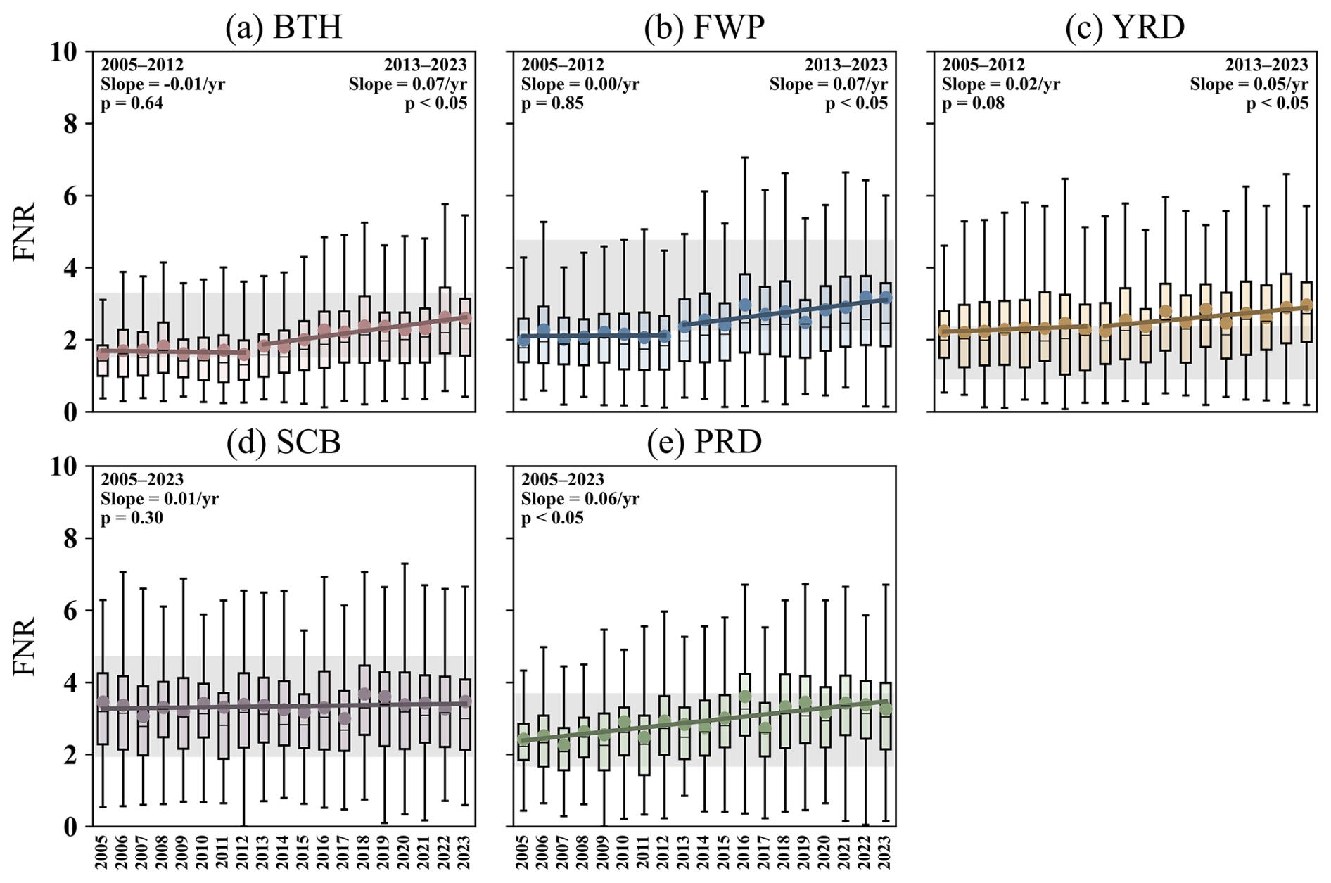
Figure 4 Interannual variations in FNR in the key regions during the warm season (April–September) from 2005 to 2023. Box plots show the median (horizontal line), the 25th and 75th percentiles (box boundaries), the minimum and maximum values (whiskers), and the mean (plus signs). The shaded areas indicate the corresponding OFS threshold ranges.

In contrast, SCB shows a relatively high annual mean FNR of 3.34 but no significant change point or clear long-term trend. In addition, SCB did not show a statistically significant change point in the Pettitt test, which further supports the decision not to interpret its FNR evolution using the same two-stage framework. Together with the relatively small changes in both NO₂ and HCHO, this suggests that the precursor structure in SCB remained comparatively stable over the study period, and OFS stayed largely within the transitional regime.

PRD differs from the other two patterns by exhibiting a significant long-term increase in FNR, at a rate of 0.06 yr⁻¹ (p < 0.05). This trend indicates a shift in OFS from VOC-limited or transitional regimes toward more NO_x-limited regimes, likely associated with reductions in NO_x-rich sources in the region, particularly from road traffic and industrial emissions, as suggested by previous studies (Bian et al., 2019; Li et al., 2025).

The timing of the detected change points broadly coincides with the implementation of major clean-air policies in China, suggesting that precursor control patterns in the major urban clusters changed substantially after the early 2010s. At the same time, under conditions of climate warming and enhanced radiation, and against the background of anthropogenic precursor reductions, continued increases in HCHO may have further promoted the shift toward more NO_x-limited chemistry (Itahashi et al., 2022; Wu et al., 2020).

3.3.2 Spatial distribution patterns of ozone formation sensitivity regimes

Based on the OMI-derived FNR, OFS in China during the warm season from 2005 to 2023 shows a clear spatial pattern (Fig. 5). VOC-limited regimes are concentrated mainly in eastern urban clusters, whereas NO_x-limited regimes are more common in surrounding suburban and less developed areas. In regions such as BTH and FWP, strong anthropogenic NO_x emissions lead to relatively low FNR values, resulting in predominantly VOC-limited regimes in most years. Away from urban cores, NO_x emissions gradually decrease, while the relative contribution of BVOCs becomes more important, leading to higher FNR values and a shift toward NO_x-limited regimes (Zhang et al., 2017; Wu et al., 2020). This spatial pattern is generally consistent with previous studies and reflects regional differences in emission structure, land cover, and urbanization level (Chen et al., 2020; Ren et al., 2022).

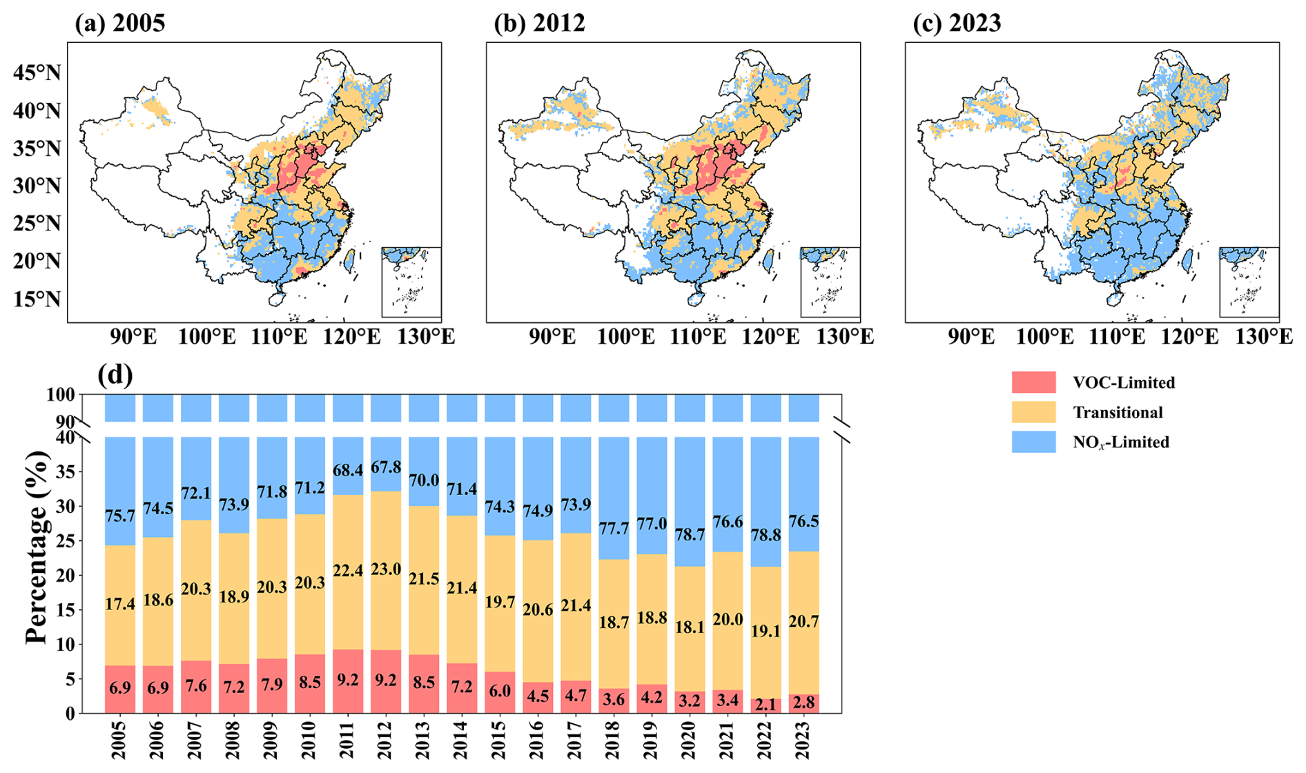
Figure 5 Spatial distribution of FNR over China during the warm season (April–September) in (a) 2005, (b) 2012, and (c) 2023; (d) interannual variation in the area fractions of different OFS regimes from 2005 to 2023. FNR is shown only for polluted regions, defined as areas with mean OMI NO₂ columns greater than 1.5 × 10¹⁵ molec. cm⁻².

The areal fractions of different OFS regimes also show a clear temporal shift before and after the implementation of the Air Pollution Prevention and Control Action Plan (Fig. 5d). During 2005–2012, the OFS distribution in eastern China shifted toward more VOC-limited regimes, mainly through transitions from NO_x-limited to transitional regimes and from transitional to VOC-limited regimes. Over this period, the area fraction of NO_x-limited regimes decreased by 7.9 %, while the fractions of transitional and VOC-limited regimes increased by 5.6 % and 2.3 %, respectively. This change is consistent with the faster increase in NO₂ than in HCHO during this period, which lowered FNR and favored VOC limitation. PRD showed a different evolution, with a decline in VOC-limited regimes and a predominance of transitional regimes by 2012.

During 2013–2023, the national OFS pattern shifted back toward NO_x-limited and transitional regimes. This change was associated with substantial reductions in NO_x emissions, comparatively slower decreases in anthropogenic VOC emissions (Fig. S5), and continued enhancement of BVOCs emissions under warmer and more strongly irradiated conditions (Zeng et al., 2023; Zhang et al., 2025a). By 2023, VOC-limited regimes accounted for only 2.8 % of the total area, whereas NO_x-limited regimes expanded to 76.5 %. This evolution indicates that OFS in China did not change monotonically over time but instead underwent a pronounced reversal under the combined influence of emission-control policies and climate-related factors (Fang et al., 2026). It also highlights the asymmetric reduction of O₃ precursors during China's clean-air actions and the resulting shifts in regional O₃ chemistry.

3.3.3 Impact of short-term COVID-19 lockdown on ozone formation sensitivity regimes

The nationwide COVID-19 lockdown in early 2020 caused a sharp but short-lived reduction in anthropogenic emissions and provided a useful case for examining the response of OFS to abrupt emission changes. To capture this process, the period was divided into three phases: pre-lockdown (1–22 January 2020; 22 d), during lockdown (23 January–13 February 2020; 22 d), and post-lockdown (14 February–7 March 2020; 23 d).

Figure 6 shows the spatial distributions of O₃ precursors and FNR during these three phases. Before the lockdown, high tropospheric NO₂ columns formed a continuous belt across the urban-industrial regions of North, East, and South China. During the lockdown, both the intensity and spatial extent of high NO₂ decreased markedly, consistent with strong reductions in industrial activity and traffic emissions. In the post-lockdown phase, NO₂ columns recovered partially in many regions, although they remained below pre-lockdown levels (Qiao et al., 2022; Zhao et al., 2022). HCHO showed a broadly similar pattern, but its spatial changes were less uniform. During the post-lockdown phase, HCHO increased over parts of South and Southwest China. This increase was likely related to the combined influence of wildfire emissions from Myanmar and northern Vietnam and enhanced BVOCs emissions (Stavrakou et al., 2021). These results suggest that seasonal and BVOCs sources played an important role in sustaining HCHO levels and increasing FNR during this period.

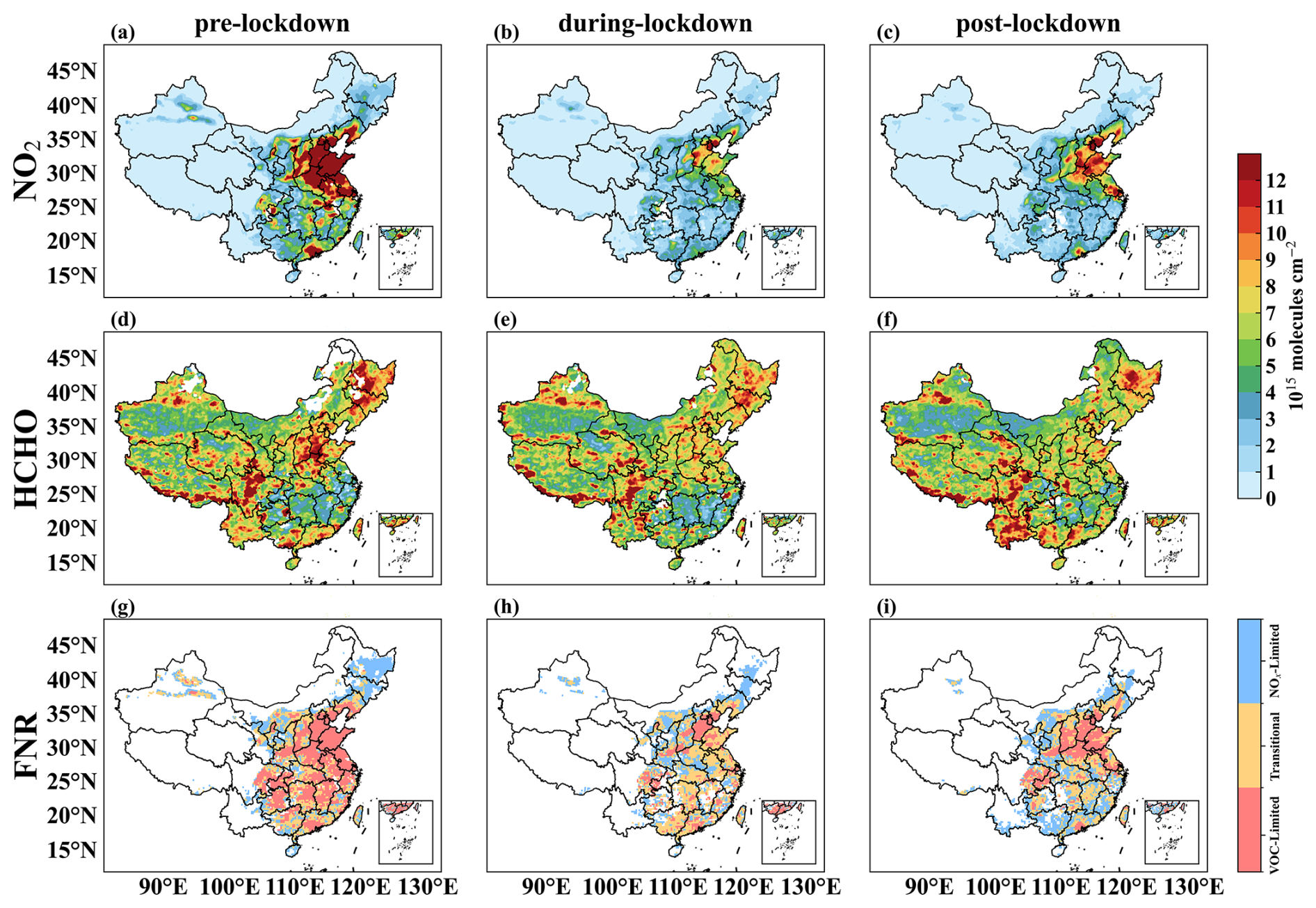
Figure 6 Spatial patterns of tropospheric NO₂ and HCHO columns, and FNR during the pre-, during-, and post- lockdown phases of early 2020. FNR is shown only for polluted regions, defined as areas with mean OMI NO₂ columns greater than 1.5 × 10¹⁵ molec. cm⁻².

The corresponding OFS distributions also changed substantially across the three phases. Before the lockdown, VOC-limited and transitional regimes dominated most major urban regions in eastern China. During the lockdown, the sharp decline in NO₂ led to a rapid increase in FNR and a broad expansion of NO_x-limited regimes. This shift was especially evident in PRD and YRD, where OFS changed rapidly from VOC-limited toward transitional or NO_x-limited regimes. Such changes are consistent with strong NO_x reductions that weakened urban O₃ titration and altered precursor limitation. In the post-lockdown phase, as NO_x emissions partly recovered, parts of the North China Plain and northern YRD shifted back toward VOC-limited and transitional regimes. However, the spatial extent of these regimes did not return to pre-lockdown levels.

The short-term OFS response during the COVID-19 lockdown is broadly consistent with the longer-term evolution observed from 2005 to 2023. In both cases, rapid reductions in NO_x promoted a shift toward more NO_x-limited regimes, whereas partial NO_x recovery or enhanced VOC emissions tended to move OFS back toward transitional or VOC-limited regimes. These results indicate that OFS in China is highly sensitive to short-term emission perturbations, especially under meteorological conditions favorable for photochemical production. They also suggest that the effectiveness of O₃ control depends strongly on precursor reduction pathways and background climatic conditions. In warm-season urban regions, sustained NO_x reductions are more likely to support O₃ mitigation, whereas coordinated VOC control remains important in regions or periods where OFS may shift back toward transitional or VOC-limited regimes.

3.4 Attribution of factors influencing OFS via explainable machine learning

3.4.1 Performance of RF models for OFS classification

Table 1 presents a comparison of the five model configurations. Overall, all models demonstrate relatively high classification performance, with AS, GMS, and ROC-AUC all exceeding 0.70. Among the regions, the models for the YRD and PRD perform the best, with all category-specific metrics generally above 0.70.

Table 1 Performance metrics of the optimized model on the validation dataset.

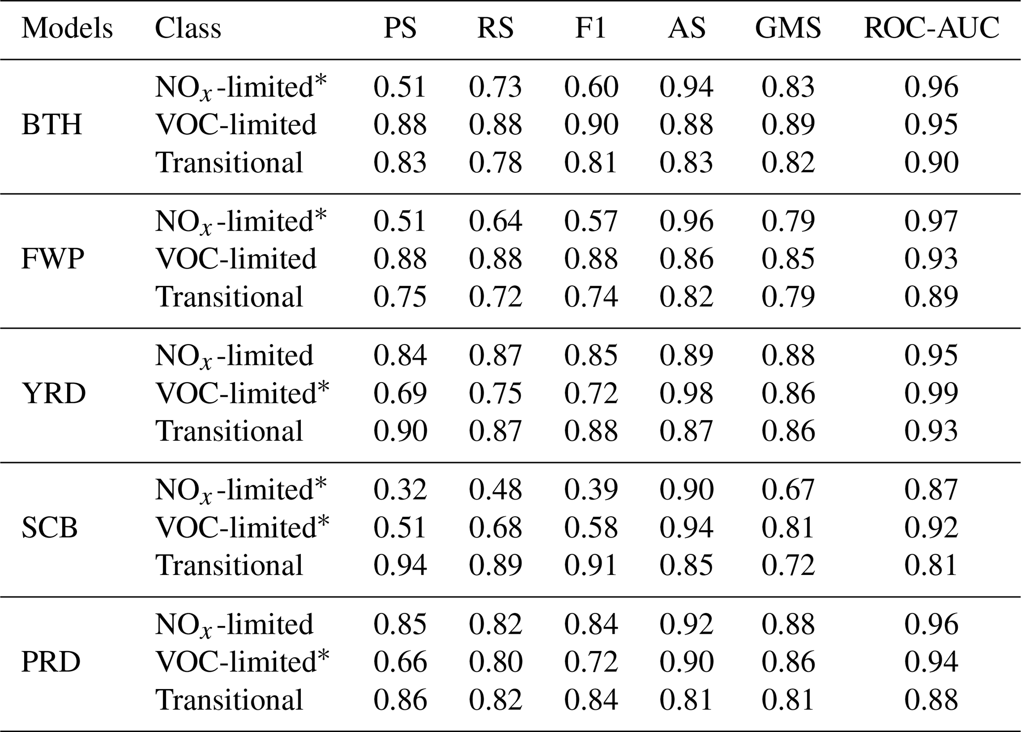
^* Minority classes (categories with fewer samples).

In contrast, the BTH and FWP models show relatively low performance for minority classes, particularly the NO_x-limited category, with F1 scores of 0.60 and 0.57, respectively, while other categories generally achieve metrics above 0.60, indicating moderate performance in identifying this category. In the SCB model, the NO_x-limited category performs the worst, with PS, RS, and F1 all below 0.50, reflecting the difficulty for the model in effectively capturing its characteristics.

Overall, after sampling and hyperparameter optimization, the models achieve robust performance on the majority classes, but classification performance for minority classes remains limited. Ahmed et al. (2025) noted that SMOTE can effectively improve classification performance by addressing data imbalance, but it may also lead to decreased accuracy for majority classes, highlighting the trade-offs involved when handling imbalanced datasets.

3.4.2 Relative contributions and regional heterogeneity of OFS influencing factors

For each regional model, SHAP values were first calculated for each sample and for each OFS class. For each class, mean(|SHAP|) was then computed for each feature across all samples, and these class-specific mean(|SHAP|) values were subsequently averaged across the three OFS classes to represent the overall importance of each feature in that regional model. To facilitate comparison among regions, the resulting overall mean(|SHAP|) values were further normalized and expressed as relative contribution percentages. Figure 7 shows the relative contribution of each feature to OFS classification in the five city clusters. Overall, emission-related variables contribute more than meteorological variables, with their total contribution ranging from 50.1 % in YRD to 72.2 % in PRD. This result indicates that OFS classification is primarily constrained by emission-related factors in most city clusters. In YRD, meteorological and emission-related variables contribute almost equally to OFS classification, accounting for 49.9 % and 50.1 %, respectively.

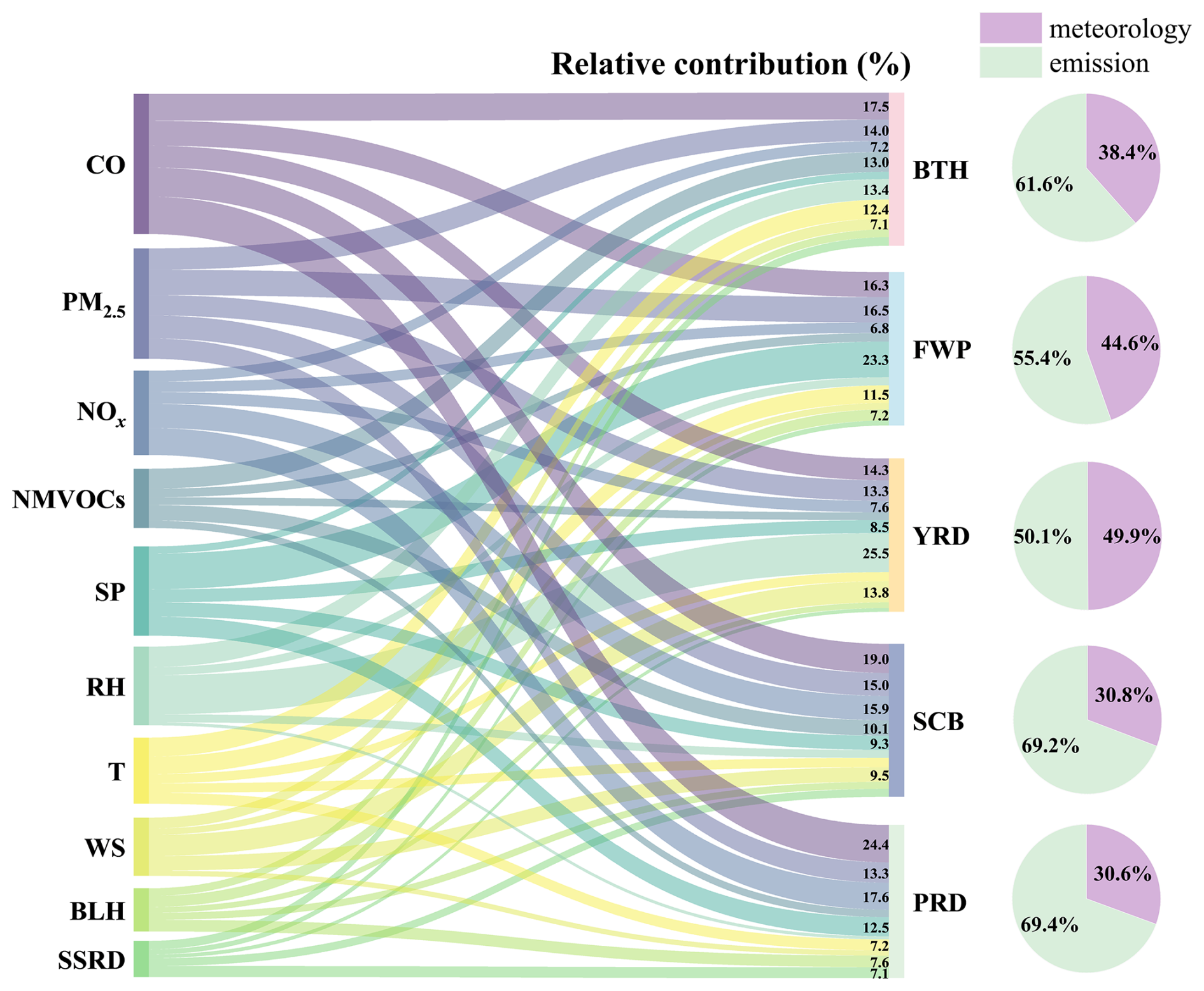
Figure 7 Relative contribution of emission-related and meteorological factors to overall OFS classification.

A closer examination of individual emission predictors reveals substantial regional heterogeneity. In BTH, FWP, and YRD, CO and PM_2.5 make the largest contributions (17.5 % and 14.0 % in BTH; 16.3 % and 16.5 % in FWP; 14.3 % and 13.3 % in YRD). NMVOCs also show a relatively large contribution in BTH, reaching 13.0 %. By contrast, SCB and PRD are characterized by high contributions from CO and NO_x (19.0 % and 15.9 % in SCB; 24.4 % and 17.6 % in PRD). The strong model importance of CO and PM_2.5 likely reflects both the influence of their significant long-term trends in the model and their broader association with regional photochemical environments. First, both variables show a two-stage trend in most urban clusters from 2005 to 2023, with an initial period of non-significant change followed by a significant decline (Fig. S5), a pattern that is similar to the phase-like changes in OFS identified in this study (Fig. S6). Second, CO can enhance hydroperoxy radical (HO₂) production through the reaction CO + OH → HO₂, thereby increasing O₃ production efficiency under conditions of declining NO_x (Ren et al., 2013; Seinfeld and Pandis, 2016). Third, a reduction in PM_2.5 may weaken its heterogeneous uptake of hydroxyl radicals (HO_x) and NO_x and thus allow more radicals and reactive nitrogen to remain available for photochemical O₃ reactions (Li et al., 2019). Therefore, these results suggest that CO and PM_2.5 function not simply as co-emitted pollutants, but also as informative predictors of broader changes in oxidation capacity and regional pollution conditions.

Meteorological predictors also show robust and regionally distinct contributions. Surface pressure (SP), relative humidity (RH), and temperature (T) are consistently important across regions, highlighting the roles of weather system stability, moisture conditions and thermal conditions in modulating photochemistry and pollutant accumulation. In the YRD, the contribution of RH is particularly notable (25.5 %), while in the FWP, SP contributes more substantially (23.3 %), indicating that OFS in these regions is also strongly influenced by meteorological factors. More broadly, meteorological factors can influence atmospheric oxidation capacity, boundary-layer structure, and pollutant dispersion, thereby shaping both the spatial distribution and temporal evolution of OFS. Therefore, the relatively high contributions of certain meteorological factors in the YRD and FWP may reflect a greater sensitivity of OFS classification to regional humidity and atmospheric stability conditions.

3.4.3 Regional and temporal shifts in OFS-related factor contributions

To further characterize the temporal evolution of the factors influencing OFS, we compared the relative contributions of emission-related and meteorological variables between the warm-season periods of 2005–2012 and 2013–2023 (Fig. 8). Overall, emission-related variables remained the dominant predictors across most urban clusters and OFS categories in both periods, with their contributions generally exceeding 50 %. This suggests that the long-term evolution of OFS in China was primarily governed by changes in precursor emissions, although the relative role of meteorology varied by region and OFS category.

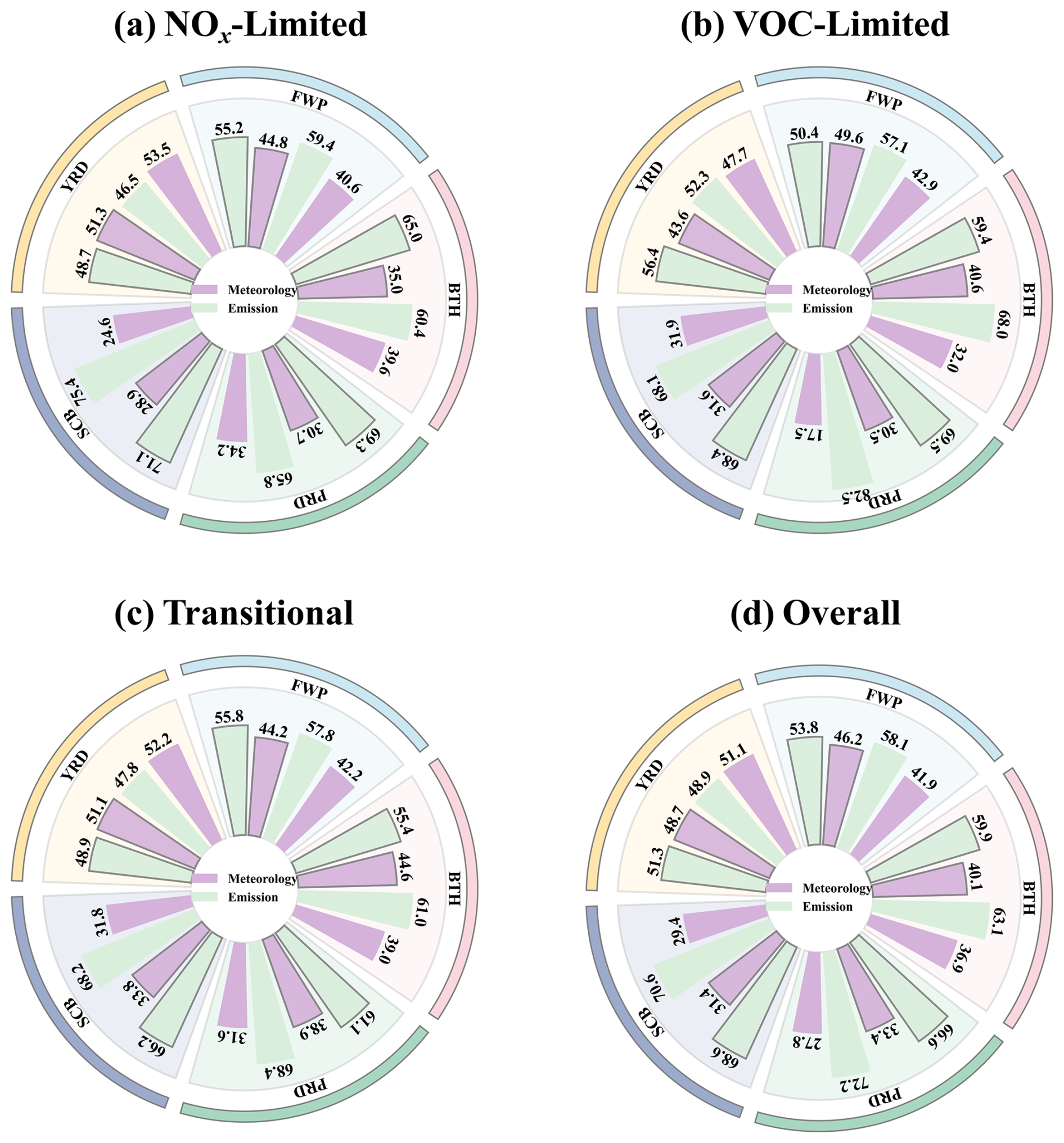
Figure 8 Relative contributions (%) of emission-related and meteorological factors to OFS classification in five urban clusters during the warm season (April–September) for the periods of 2005–2012 and 2013–2023, shown separately for (a) NO_x-limited, (b) VOC-limited, (c) transitional, and (d) overall OFS states. Gray outlined bars denote 2013–2023, whereas bars without outlines denote 2005–2012.

For the NO_x-limited regime, the contributions of meteorological and emission-related factors in YRD were broadly comparable, whereas emission-related contributions in BTH, YRD, and PRD increased slightly after 2013 (+4.6 %, +2.2 %, and +3.5 %, respectively). By contrast, meteorological contributions increased moderately in FWP and SCB (+4.2 % and +4.3 %, respectively). In the VOC-limited and transitional regimes, emission-related factors also remained dominant overall. However, meteorological contributions to the VOC-limited regime increased markedly after 2013 in BTH, FWP, and PRD, by +8.6 %, +6.7 %, and +13.0 %, respectively. For the transitional regime, meteorological contributions increased in all urban clusters except YRD, accompanied by corresponding declines in emission-related contributions of approximately 2.0 %–7.3 %.

From an overall perspective (Fig. 8d), the relative contribution of emission-related factors decreased slightly after 2013 in BTH, FWP, SCB, and PRD, by about 2.0 %–5.6 %. In YRD, the relative contributions of meteorological and emission-related factors remained broadly comparable, although the balance shifted slightly toward emission-related influences after 2013. Taken together, these results indicate that, while OFS classification remained predominantly emission-driven, the regulatory role of meteorology became more pronounced after 2013. This pattern suggests a modest transition from a regime controlled mainly by emissions toward one jointly modulated by emissions and meteorological conditions. Such a shift is consistent with the substantial reduction in precursor emissions after 2013 and implies that, under a cleaner emission background (Fig. S5), OFS classification may become increasingly sensitive to meteorological variability.

These findings are broadly consistent with previous regional studies, while also highlighting the strong spatial heterogeneity of OFS influencing factors across China. In the Guangdong–Hong Kong–Macao Greater Bay Area, FNR has been reported to be mainly influenced by temperature, shortwave radiation, total column water, and surface pressure (Chen et al., 2020), whereas in Guangdong Province it is primarily associated with surface solar radiation, relative humidity, and temperature (Liang et al., 2024b), although emission-related variables were not explicitly considered. By contrast, in the Chengdu–Chongqing region, summer OFS has been shown to be mainly driven by CO, PM_2.5, NMVOCs, and NO_x emissions, with increasing pollution shifting OFS toward VOC-limited regimes (Xu et al., 2025). In the North China Plain, the decline in PM_2.5 concentrations reduces the loss of HO₂, enhances their reaction with NO, thereby strengthening NO_x sensitivity and leading to increased O₃ levels (Li et al., 2019). Together, these studies support the view that OFS evolution reflects the combined influence of emissions and meteorology, but that their relative roles differ substantially among regions. Compared with these regional analyses, our results provide a unified national-scale framework showing that emission-related factors generally dominate OFS classification, while meteorological modulation becomes more evident under a cleaner emission background.

3.4.4 SHAP responses of individual predictors across OFS regimes

To further interpret how individual predictors influence OFS classification, we examined the SHAP value distributions of different variables for each urban cluster (Fig. 9). The results reveal both common features and regional differences in the directional and nonlinear effects of the predictors. In general, many variables show broadly opposite SHAP responses between VOC-limited and NO_x-limited regimes, indicating that the same predictor can exert contrasting effects under different chemical sensitivity conditions.

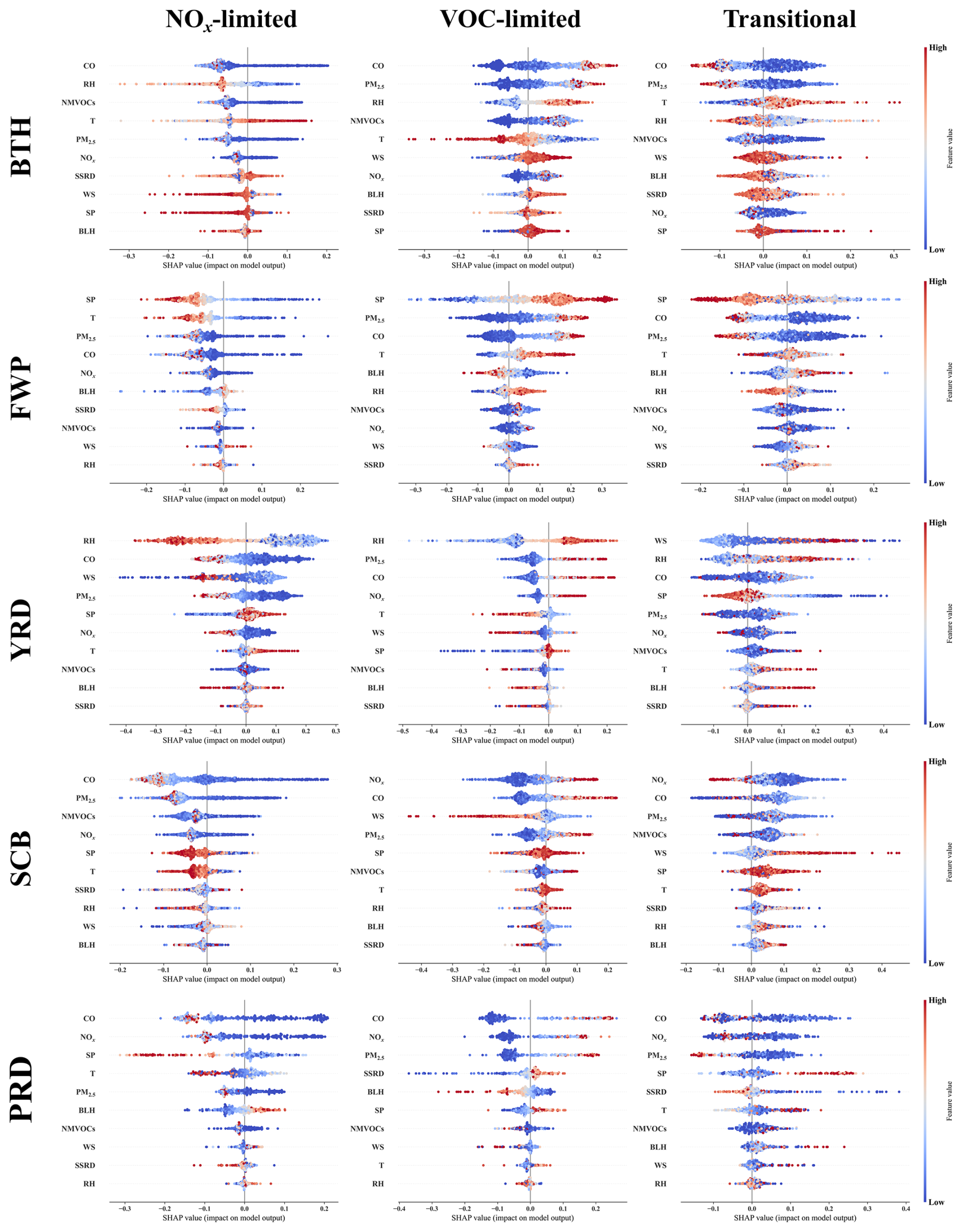
Figure 9 SHAP value distributions of individual predictors in the RF models for the five urban clusters in China.

For emission-related variables, samples classified as NO_x-limited are generally associated with relatively low emission levels. By contrast, under VOC-limited regimes, higher emission values are more consistently associated with positive SHAP values, indicating a greater probability of being classified as VOC-limited. This pattern is broadly consistent with the spatial distribution of OFS, in which NO_x-limited regimes are more common in suburban or peripheral areas, whereas VOC-limited regimes are concentrated in urban cores with stronger anthropogenic emissions (Xue et al., 2014; Wang et al., 2021; Johnson et al., 2024). Overall, the regional differences in the SHAP responses of emission variables likely reflect differences in local emission intensity and chemical sensitivity.

Meteorological variables also show substantial but regionally distinct effects on OFS classification. SP, RH, and T emerge as influential predictors in several regions, but their directional effects vary geographically. In BTH and YRD, higher temperatures are more closely associated with NO_x-limited classification, which may reflect enhanced photochemical activity and BVOCs emissions under warm conditions (Pétron et al., 2001; Duncan et al., 2009). In several other regions, however, higher temperature is more often linked to VOC-limited classification, which may also be related to the spatial distribution of urban heat islands (Zhou et al., 2015). SP influences pollutant accumulation and vertical mixing through atmospheric stability and subsidence; in general, higher SP favors VOC-limited classification, whereas lower SP is more closely associated with NO_x-limited regimes, with particularly asymmetric SHAP responses in YRD. RH is especially important in BTH and YRD, where high humidity tends to promote VOC-limited classification. Higher relative humidity may promote aerosol growth, thereby reducing the radiation reaching the surface and limiting the photochemical production of HCHO (Ye et al., 2016).

Compared with VOC-limited and NO_x-limited regimes, the transitional regime shows less consistent directional responses across variables and regions. This suggests that transitional regimes are governed by a more complex combination of emissions and meteorological influences, with stronger nonlinearity and greater classification uncertainty. Such complexity implies that transitional regimes may be the most difficult to manage using simple precursor-reduction strategies alone and may require more detailed process-based analysis to support effective control design.

Overall, the SHAP analysis highlights that OFS classification is shaped by both shared and region-specific predictor responses. Emission-related variables remain the dominant contributors in most regions, whereas meteorological variables modulate the OFS transitions in a region-dependent manner. These results provide a more process-informed interpretation of the regional heterogeneity and temporal evolution of OFS across China during the warm season.

4 Conclusion

This study developed an observation-constrained and interpretable framework to diagnose the long-term evolution of OFS across China during the warm season (April–September) from 2005 to 2023. By combining OMI observations of NO₂ and HCHO with ground-based O₃ measurements, we derived region-specific FNR threshold ranges and used them to characterize the spatial and temporal evolution of OFS. We further coupled RF models and SHAP analyses to quantify the relative roles of emission-related and meteorological factors in OFS classification.

The long-term evolution of O₃ precursors showed a pronounced divergence after 2013: NO₂ declined substantially under strengthened emission-control policies, whereas HCHO continued to increase in many regions. This asynchronous evolution substantially reshaped FNR and provided the precursor basis for subsequent OFS shifts. At the same time, the derived FNR threshold ranges differed markedly across regions, demonstrating that a uniform national threshold is insufficient for OFS diagnosis in China, and that region-specific thresholds provide a more robust basis for reducing classification uncertainty.

Against this background, OFS over China exhibited a clear phase-dependent evolution. During 2005–2012, many regions shifted from NO_x-limited toward transitional or VOC-limited regimes as NO₂ increased. After 2013, the sharp decline in NO₂ together with a modest rise in HCHO drove a widespread return toward more NO_x-limited chemistry, especially in eastern China. However, this transition was not spatially uniform and exhibited a clear temporal shift around 2013, with BTH and FWP shifting from VOC-limited toward transitional regimes, and YRD evolving toward NO_x-limited regimes. SCB remained in largely transitional regimes, while PRD shifted from transitional toward NO_x-limited regimes. These results indicate that OFS in China has undergone a policy-related but regionally heterogeneous restructuring over the past two decades.

Although the definition of OFS is based on the relative proportions of precursors, its spatiotemporal patterns actually reflect the combined effects of emission sources and meteorological conditions. Therefore, we treat OFS types as integrated response states and apply ML techniques to statistically model their relationships with meteorological parameters and emission variables. Within this framework, meteorological factors indirectly influence the formation of OFS by modulating the probabilities of different OFS states, rather than directly altering the FNR definition itself. Our focus is on the FNR-derived OFS, rather than absolute O₃ concentrations, enabling us to elucidate how meteorology governs the classification and evolution of sensitivity regimes. It should be noted that the attribution analysis presented here is based on statistical associations, and the results only reflect the relative contributions of each variable to OFS states, without implying strict causal relationships.

The explainable ML analysis further showed that emission-related variables remained the dominant predictors of OFS classification in most regions, whereas meteorological factors exerted region-dependent modulation of the direction and strength of OFS transitions. After 2013, the relative influence of meteorology increased modestly in several regions, suggesting that under a cleaner emission background, OFS becomes more sensitive to meteorological variability. Overall, these findings indicate that the long-term evolution of OFS in China is primarily driven by emission changes but increasingly modulated by meteorological conditions.

This study is subject to several uncertainties and limitations. First, this is an exploratory application of a classification model to OFS states, and the performance of the RF depends on class balance; however, the threshold-based classification leads to class imbalance, and some influencing factors are not included. Second, the thresholds themselves are uncertain, and the coarse spatial resolution of OMI data, along with mismatches with ground observations, may introduce classification uncertainty and affect model performance. The use of higher-resolution data such as TROPOMI, combined with O₃ observations, can improve diagnostic accuracy (Ren et al., 2022). Future work integrating ML with observations and chemical transport models may help bridge this gap (Xiong et al., 2024). Therefore, the present framework should be viewed as a complementary statistical attribution tool, rather than a substitute for process-based OFS diagnosis using chemical transport models or observation-based box models.

In summary, this study derived region-specific FNR threshold ranges and revealed pronounced spatial differences in OFS classification across China, providing a more robust basis for refined O₃ control. The results further show that the long-term evolution of OFS is primarily shaped by emission changes, while regional meteorological conditions increasingly modulate its spatial distribution and temporal transitions under a cleaner emission background. These findings indicate that future OFS assessments and control strategies should account not only for precursor reductions, but also for regional meteorological variability and the coupled interactions among NO_x, NMVOCs, PM_2.5, and CO. Overall, the satellite–indicator (FNR)–interpretable machine learning (RF + SHAP) framework developed here provides a scalable and decomposable framework for interpreting the long-term evolution and associated factors influencing FNR-derived OFS states from national to urban-cluster scales. This framework offers a useful scientific basis for dynamic sensitivity reclassification and the design of region-specific NO_x–VOC control strategies, with broader relevance for O₃ mitigation in other megacity regions.