Global Observations and European emissions of the halogenated olefins HFO-1234yf, HFO-1234ze(E), and HCFO-1233zd(E) from the AGAGE (Advanced Global Atmospheric Gases Experiment) network

Hydrofluoroolefins (HFOs) are important synthetic compounds replacing other halocarbons in phase-down from usage (e.g., as refrigerants, propellants, foam blowing). Little is known about their atmospheric abundance, distribution and trends, nor about their emissons. Here, we report atmospheric observations of the widely used HFO-1234yf (2,3,3,3-tetrafluoroprop-1-ene), and HFO-1234ze(E) (E-1,3,3,3-tetrafluoroprop-1-ene), and the hydrochlorofluoroolefin (HCFO) HCFO-1233zd(E) (E-1-chloro-3,3,3-trifluoroprop-1-ene) observed as part of the Advanced Global Atmospheric Gases Experiment (AGAGE) network. Over the observational period 2011–2025, pollution events have grown in magnitude and frequency at sites which are influenced by regional emissions, while remote stations show first appearances of these substances. By 2024/2025 winter peak mole fractions in background northern hemisphere air have reached ∼ 0.25 ppt (picomol mol⁻¹, parts-per-trillion in dry air) for HFO-1234yf and HFO-1234ze(E) and ∼ 0.45 ppt for HCFO-1233zd(E). Using European observations and the inverse modeling frameworks InTEM, ELRIS, and RHIME we determine emission trends and regional distributions. For Northwest Europe, emissions of HFO-1234yf increased steadily and rapidly from <0.1 Gg yr⁻¹ in 2014 to 1.50 [1.23–1.74, range of 16–84 percentile] Gg yr⁻¹ by 2023, presumably due to its introduction in mobile air conditioning and stationary refrigeration. HFO-1234ze(E) emissions were low during 2014–2017, followed by a rapid increase in 2018/2019, potentially due its introduction as an aerosol propellant, after which they increased more slowly to 0.96 [0.82–1.13] Gg yr⁻¹ by 2023. HCFO-1233zd(E) emissions are derived from 2017 onward, showing a steady increase from 0.15 [0.07–0.23] to 1.04 [0.93–1.15] Gg yr⁻¹ in 2023.

1 Introduction

Synthetically produced halocarbons have undergone several replacement and phase-out periods over the past decades. Their use in refrigeration, foam blowing, fire suppression, and solvent applications has led to emissions to the atmosphere, where they are involved in stratospheric ozone depletion and infrared radiation absorption, contributing to the enhanced greenhouse gas effect. The production and use of first generation halocarbons, e.g., chlorofluorocarbons (CFCs) and halons, have been largely phased out under the Montreal Protocol on Substances That Deplete the Ozone Layer since they deplete stratospheric ozone. Similarly, the transitional second generation hydrochlorofluorocarbons (HCFCs) have largely been phased out under the Montreal Protocol. The third generation products, hydrofluorocarbons (HFCs), do not destroy stratospheric ozone, but are strong greenhouse gases and hence were included in the Kigali Amendment to the Montreal Protocol in 2016 (United Nations, 2016) for a phase-down over the next decades. HFCs are currently being replaced by compounds with lower global warming potentials (GWP), including haloolefins. These are halogenated organic substances with an unsaturated carbon-carbon bond, resulting in a much shorter atmosphere lifetime compared to saturated halocarbons (order of days to weeks, compared to years to decades). Hence, their GWP and their Ozone Depletion Potential (ODP) are small. Even though some environmental concerns exist, haloolefins are currently not included in the Montreal Protocol.

The subjects of the present study are atmospheric observations and derived emissions of the most widely used hydrofluoroolefins (HFOs): HFO-1234yf (2,3,3,3-tetrafluoroprop-1-ene, CF₃CF=CH₂, CAS No. 754-12-1), and HFO-1234ze(E) (E-1,3,3,3-tetrafluoroprop-1-ene, trans-CF₃CH=CHF, CAS No 29118-24-9) and the hydrochlorofluoroolefin (HCFO) HCFO-1233zd(E) (E-1-chloro-3,3,3-trifluoroprop-1-ene, trans-CF₃CH=CHCl, CAS No. 102687-65-0). The three substances are mainly used in refrigeration, air conditioning, heat pumps (RACHP), and/or foam blowing. However, given the lack of reliable literature, it is difficult to evaluate the individual sectors in more detail, and also difficult to comprehensively reconstruct regulations and applications and the changes thereof for individual countries or regions.

In the European Union (EU) for example, haloolefins are included in the Regulation on fluorinated greenhouse gases 2024/573 (“2024 F-gas Regulation”, European Parliament and Council (2024)). Due to their low GWP, they are currently not included in the regulation's phase-down of consumption, but they will be banned in various applications starting 2035 due to environmental concerns. In addition, emissions prevention and recovery regulations (Article 4) and recycling and destruction regulations (Article 8) will apply to haloolefins. Haloolefins are also within the scope of the definition of the very stable anthropogenic per- and polyfluoroalkyl substances (PFAS). In January 2023, authorities from Denmark, Germany, the Netherlands, Norway, and Sweden submitted a REACH (Registration, Evaluation, Authorisation and Restriction of Chemicals) dossier for a restriction proposal for PFAS in the EU to the European Chemicals Agency (ECHA) (ECHA, European Chemicals Agency, 2025). It suggests a wide-ranging ban of PFAS from usage in many applications. At the time of publication of our article, this dossier is still being discussed by the ECHA.

The predominant degradation pathway of this study's haloolefins from the atmosphere is initiated via reaction with the hydroxyl radical, while reaction with ozone and chlorine are negligible under environmental conditions (Nielsen et al., 2007; Søndergaard et al., 2007; Sulbaek Andersen et al., 2008, 2012; Madronich et al., 2023; Tewari et al., 2025). These compounds undergo complex atmospheric decay processes and there are concerns of harmful degradation products. In particular the formation of trifluoroacetic acid (TFA) is under active debate (Henne et al., 2012; Lindley et al., 2019; Behringer et al., 2021; David et al., 2021; Arp et al., 2024; Khan et al., 2026; Tewari et al., 2025; Henne et al., 2025; Hart et al., 2026). TFA is toxic and very stable under environmental conditions, raising concerns of accumulation in the environment. There is also an active debate on the potential atmospheric degradation pathway to the potent greenhouse gas fluoroform (HFC-23) (Sulbaek Andersen and Nielsen, 2022; McGillen et al., 2023; Pérez-Peña et al., 2023; Thomson et al., 2025; Van Hoomissen et al., 2025). The synthesis of haloolefins is also complex with CFCs, HCFCs, and HFCs involved as precursors and intermediates (Sicard and Baker, 2020), leading to the debate of stricter control and emission reduction of these ODSs and potent greenhouse gases (Solomon et al., 2020).

Here, we provide information of usage patterns of the three haloolefins for the EU and the UK, many of which may also apply to other parts of the world, although likely at different time frames. While this information remains anecdotal (without the ability to provide peer-reviewed literature citations) and estimates are based on bottom-up consumption models, which rely on assumptions regarding inventory and release functions, it is nevertheless helpful for the interpretation of our emission estimates.

HFO-1234yf is solely used in RACHP and for 2023 an estimated 77 % of it was used in pure form as the main replacement for HFC-134a in mobile air conditioning (MAC). The remaining 23 % was used in blends (mainly R448A and R449A), which are used in stationary refrigeration units. While these blends are drop-in replacements for older HFC-based refrigerants, their total GWPs are still relatively high (∼ 1400) because they still contain significant amounts of HFCs. They are therefore projected to be replaced in the near future by lower (<150) GWP refrigerants such as R454C and R455A (79 % and 76 % HFO-1234yf, respectively).

HFO-1234ze(E) is used in RACHP, foam blowing and as an aerosol propellant but the individual shares of these three applications are poorly known to us. Usage in the RACHP sector is as pure fluid in medium-sized chillers and in refrigeration blends (R448A and R450A) with GWPs of ∼ 600 as a replacement for HFC-134a. HFO-1234ze(E) is a foam blowing replacement compound for HFCs (mainly HFC-245fa and HFC-365mfc), which are banned for this application in the EU since 2023. The quantities used and their temporal evolution are not known to us, however, it is expected that this application contributes considerably to the emissions we derive for this compound. HFO-1234ze(E) is also used as an aerosol propellant as one of the HFC-134a replacements in technical applications following the HFC-134a ban under the 2014 F-gas regulation (European Parliament and Council, 2014). A HFC-134a phase-down regulation is now also in place for metered dose inhalers (MDIs) for pharmaceutical use in the 2024 F-gas regulation (European Parliament and Council, 2024). HFO-1234ze(E) is currently tested as one potential replacement in this application. Overall, it is assumed that its application in aerosol sprays is contributing considerably to emissions in Europe, particularly as this application is fully emissive.

HCFO-1233zd(E) was originally marketed as a solvent but is now mainly used as foam blowing agent and in minor quantities in RACHP. The former is currently assumed to be the major emission source in the EU. With the ban of HCFC-123 in the EU in 2000, alternative refrigerants for large-scale low-pressure chillers were not available resulting in the use of different technologies. This situation changed recently when HCFO-1233zd(E) was identified as suitable for these chillers. While their applications (and resulting HCFO-1233zd(E) emissions) are currently assumed to be small, they will likely become more significant.

As these three substances are mainly replacing the HFCs in phase-down, it is expected that the transition to these chemicals will appear first in regions with accelerated phase-down schedules in the Montreal Protocol, and those with additional regulations, particularly in Europe (EU Regulation on fluorinated greenhouse gases 2024/573 (European Parliament and Council, 2024)), in the USA (American Innovation & Manufacturing (AIM) Act of 2020 US-AIM, 2020), Canada, and Australia.

Little is currently known about the atmospheric abundance and distribution of the three compounds. Their first atmospheric measurements were reported by Vollmer et al. (2015) from the semi-remote Jungfraujoch (Switzerland) station and from an urban site in Switzerland. Starting in 2014, the measurements of the three compounds were gradually extended to most stations of the Advanced Global Atmospheric Gases Experiment (AGAGE, https://www-air.larc.nasa.gov/missions/agage/, last access: 12 May 2026) network (Prinn et al., 2018; Western et al., 2025).

Here, we present HFO and HCFO observations from most AGAGE sites to the end of 2025 and we use the dense European station network in a detailed modeling study to estimate 10 years (2014–2023) of emissions from Northwest (NW) Europe. We compare these to emission estimates of the refrigerant HFC-134a derived from AGAGE measurements, to explore the transition from HFC-134a to the three haloolefins, in particular in the MAC sector (O'Doherty et al., 2004; Manning et al., 2021; Liang et al., 2022).

Because of the spatial sparsity of the observations in the AGAGE network we are currently unable to conduct other regional estimates. In addition, unlike the long-lived halocarbons, global or hemispheric emissions estimates using the AGAGE 12-box model (Cunnold et al., 1983; Rigby et al., 2013; Western et al., 2025) are not feasible due to the short atmospheric lifetimes of the haloolefins.

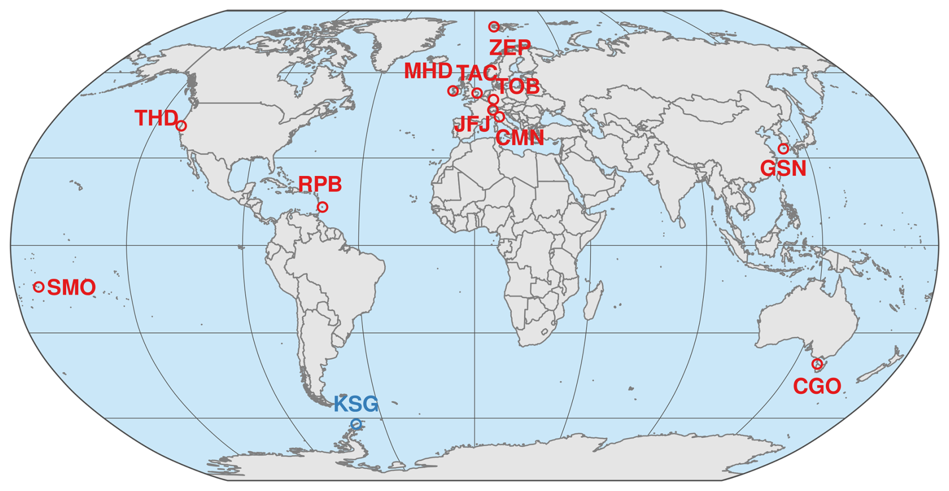
Figure 1 Location of the AGAGE (Advanced Global Atmospheric Gases Experiment) stations (in red) with publicly available measurements of HFO-1234yf (CF₃CF=CH₂), HFO-1234ze(E) (trans-CF₃CH=CHF), and HCFO-1233zd(E) (trans-CF₃CH=CHCl): Zeppelin, Spitsbergen (ZEP), Mace Head, Ireland (MHD), Tacolneston, UK (TAC), Taunus, Germany (TOB), Jungfraujoch, Switzerland (JFJ), Monte Cimone, Italy (CMN), Trinidad Head, California, USA (THD), Gosan, South Korea (GSN), Ragged Point, Barbados (RPB), Cape Matatula, American Samoa (SMO), and Kennaook/Cape Grim, Australia (CGO). Flask sample measurements are available from the South Korean Antarctic station King Sejong (in blue).

Table 1 Station List and Data Availability for HFO-1234yf (CF₃CF=CH₂), HFO-1234ze(E) (trans-CF₃CH=CHF), and HCFO-1233zd(E) (trans-CF₃CH=CHCl)^a.

^a Stations are listed in latitudinal order from north to south. Data availability for in situ and flask records with start and end dates. Abbreviations are: AGAGE: Advanced Global Atmospheric Gases Experiment. KOPRI: Korea Polar Research Institute. Empa: Swiss Federal Laboratories for Materials Science and Technology. ^b These are the altitudes of the science buildings. Air intake altitudes at most stations may be higher.

2 Methods

2.1 Stations

In situ measurements of the three haloolefins are currently conducted at most AGAGE stations (Fig. 1). In Europe, measurements are conducted at Zeppelin (Ny Ålesund, Spitsbergen, Norway), Mace Head (Ireland), Tacolneston (UK), Jungfraujoch (Switzerland), Monte Cimone (Italy, recent instrument upgrade, see also Supplement) and most recently at Taunus (Germany, Meixner et al., 2025). They are also measured at Trinidad Head (California, USA), Gosan (Jeju Island, South Korea), Ragged Point (Barbados), Cape Matatula (American Samoa), and Kennaook/Cape Grim (Tasmania, Australia), see Table 1. We also provide measurements of samples collected weekly at the South Korean Antarctic station King Sejong (South Shetland Islands) and analyzed at the Swiss Federal Laboratories for Materials Science and Technology (Empa), see Supplement Sect. S3.

2.2 Analytical Setup

Measurements reported here are mostly based on Medusa gas chromatography mass spectrometry (GCMS) techniques (Miller et al., 2008; Arnold et al., 2012; Prinn et al., 2018). The Medusa-GCMS instruments at Monte Cimone and Taunus were recently built and installed (Table 1). These are the first commercially available Medusa-GCMS instruments (Markes International, UK), designed to closely follow the AGAGE custom built Medusa-GCMS instruments in functionality and operation. At Monte Cimone, haloolefins were already measured since 2017 using different instrumentation (Maione et al., 2013), and in overlap with Medusa-GCMS (October 2022–December 2023), see Sect. S8.

On the Medusa-GCMS, typically a 2 L sample is pre-concentrated on a first cold trap filled with HayeSep D at −160 °C before it is cryo-focused onto a second trap at similar temperature. In this process, remnants of oxygen and nitrogen and significant fractions of carbon dioxide and some noble gases are removed. The sample is then injected onto the chromatographic column (CP-PoraBOND Q, 0.32 mm ID ×25 m, 5 µm, Varian Chrompack) in the gas chromatograph (Agilent 6890 or 7890), purged with helium (grade 6.0), which is further purified using a getter (HP2, VICI, USA). The sample is detected in the quadrupole mass spectrometer in selected ion monitoring mode (initially Agilent model 5973s, later 5975/5977 models). For details on acquired fragment ions, mass spectra, retention times, and nonlinearity experiments, see Vollmer et al. (2015). On the older Monte Cimone GCMS instrument (Table 1) with a Gaspro chromatographic column, HFO-1234yf and HFO-1234ze(E) are detected ∼ 10 s before HFC-134a and Halon-1211, respectively (using $m/z$ 114 and 69) and HCFO-1233zd(E) is detected ∼8 s before HFC-245fa (using $m/z$ 130 and 95).

For most stations, the chromatograms for the measured fragments are remarkably clean from interference by other compounds, and instrument blanks and memory effects are absent. We define “detection limit” for these measurements as the mole fractions that correspond to the smallest integrated chromatographic peaks. These vary over time and among the instruments, mostly reflecting the performance status of the GCMS. Reliable detection of the peaks is estimated at mole fractions larger than ∼ 0.005 ppt (parts-per-trillion, picomol mol⁻¹), which we refer to as “detectable levels” in the Results Section.

Repeated long-term measurements of the three haloolefins from whole-air calibration standards stored in 34 L internally electropolished stainless steel canisters (Essex Industries, Missouri, USA), as typically used in AGAGE, reveal stability over years. These calibration standards are filled under “wet” conditions (no active drying of the samples; water vapor is targeted near saturation pressure) to passivate the tanks' internal surfaces to avoid degradation of some measured compounds, foremost CCl₄. Whether this is necessary to maintain stability of the haloolefins is unknown to us. Also, we found that the haloolefins were preserved during passage through Nafion driers (Permapure, US) inside the Medusa-GCMS, in particular, no memory effects were observed (unlike some other compounds with carbon-carbon double bonds, e.g., propene).

2.3 Calibration

The AGAGE calibration scheme is based on a hierarchy of whole-air standards compressed into “Essex” canisters. Secondary and tertiary standards are filled by the Scripps Institution of Oceanography (SIO) at La Jolla (California), while most quaternary/working standards (used to calibrate the individual instruments) are filled by station maintainers. All standards are generally filled under clean-air conditions using modified oil-less diving compressors (Rix Industries, USA) or cryogenic techniques. Since the abundances of these short-lived haloolefins are often very low or even absent in these air masses, which would result in a highly uncertain calibration scale propagation, the tanks are spiked with small quantities of haloolefins. This typically results in mole fractions of 0.5–1.5 ppt with chromatographic peak sizes well above detection limits. The three substances are the first (and currently only) species spiked into calibration tanks in a coordinated approach within the entire AGAGE network.

The primary calibration scales for these three substances were originally maintained by Empa (Vollmer et al., 2015). However, with the incorporation of these measurements into the AGAGE network, these scales were transferred to the AGAGE central calibration facility at SIO via the inter-comparison of a suite of calibration standards. This transfer allows for the maintenance of the calibration scales within a much larger selection of secondary reference standards at SIO and a more direct calibration of tertiary standards, which are exchanged with the field sites. These tertiary standards are used on site to propagate calibration onto the quaternary/working standards, which in turn are used to calibrate the instruments for air measurements.

For HFO-1234yf, the newly available METAS-2017 primary calibration scale (Guillevic et al., 2018) was adopted by AGAGE. It has an improved expanded uncertainty (1.5 %, 2σ) compared to the Empa-2013 calibration scale (Vollmer et al., 2015). Based on a METAS-2017/Empa-2013 calibration scale conversion factor of 0.910, all older data were updated to the new primary calibration scale. The calibrations of HFO-1234ze(E) and HCFO-1233zd(E) remain on the Empa-2013 primary scales with assigned uncertainties of 15% (1σ) (Vollmer et al., 2015).

2.4 Calibration and Measurement Uncertainties

To derive accuracies for the reported measurements we follow an approach outlined in Vollmer et al. (2018) and combine three independent uncertainties: uncertainty of the calibration scales mentioned in the previous subsection, propagation uncertainty, and the instrumental precision of the measured air sample. The propagation uncertainty combines all uncertainties arising from the inter-comparisons of the standards used to propagate assigned mole fraction in the primary standards to the on-site quaternary (working) standards. We assume that the measurement uncertainties of these standards are the same for secondary, tertiary, and quaternary standards and treat them independently. The resulting propagation uncertainties (1σ) are ∼4 % for HFO-1234yf and HFO-1234ze(E), and ∼2 % for HCFO-1233zd(E). The uncertainties directly associated with the air sample measurements on the Medusa-GCMS are highly mole-fraction dependent. For individual air samples with mole fractions up to 0.5–1 ppt, we conservatively estimate these at 0.020 ppt or 10 %, whichever is greater. For more polluted air masses with mole fractions greater than ∼1 ppt, the precisions are ∼2 % for HFO-1234yf and HFO-1234ze(E), and ∼1 % for HCFO-1233zd(E) as determined from repeated measurements of working standards of similar mole fractions. The resulting combined uncertainties for air samples with elevated mole fractions in polluted air are estimated at 7% for HFO-1234yf, and 16 %–20 % for HFO-1234ze(E) and HCFO-1233zd(E), the latter two being dominated by the large calibration scale uncertainties. For direct comparisons of measurements reported within the AGAGE network including long-term atmospheric trends, the calibration scale uncertainties do not apply and the remaining uncertainties reduce to approximately 5 %–10 % in more polluted air samples.

2.5 Inverse modeling

Three atmospheric inverse modeling systems were employed to estimate emissions of HFO-1234yf, HFO-1234ze(E) and HCFO-1233zd(E) from NW Europe (Belgium, Germany, France, UK, Ireland, Luxembourg and the Netherlands), using data from Mace Head, Tacolneston, Monte Cimone and Jungfraujoch (the Taunus observation records were deemed too brief). These systems are the Inverse Technique for Emission Modeling (InTEM, Arnold et al., 2018; Manning et al., 2021), the Regional Hierarchical Inverse Modeling Environment (RHIME, Ganesan et al., 2014), and Empa's Lagrangian Regional Inversion System (ELRIS, Henne et al., 2016; Katharopoulos et al., 2023). Each system utilizes output from an atmospheric transport model and a Bayesian optimization framework to estimate spatially-resolved emissions on a reduced resolution grid determined by the observation network. Total mole fractions are simulated as the sum of a regional fraction, determined by the emissions and the regional transport model, and a background contribution (boundary condition). The Bayesian approach minimizes the mismatch between the simulated and the observed atmospheric mole fractions, taking into account both the constraints imposed by the observation and model uncertainties and the uncertainties associated with a priori emissions.

All three systems have been applied in previous studies (e.g., Redington et al., 2023) and are only briefly described below, first in terms of their common aspects (transport model and prior emissions) and then individually for where they differ. In all cases observations were first averaged into 4 h periods and individual inversions were performed independently for individual years, assuming constant emissions over the course of a year (no seasonality or trend considered). Because of the occasionally low abundance of the haloolefins in air samples, chromatographic peaks were frequently not integrated (Sect. 2.2), so the reported mole fraction was zero (despite occasional positive but not integrated above-baseline detector responses). For the purpose of inverse modeling, all observations with reported mole fractions below 0.0025 ppt (i.e. half the limit of detection) were set to 0.0025 ppt. A posteriori emissions are presented without further temporal smoothing/aggregation (except the HFC-134a estimates taken from a previous study, which are presented with a 3-year rolling-average applied).

The selection of countries for which emissions are reported was based on the country-level error reduction for the inversion posterior emissions. This depends on the spatial sensitivity of the observation network, which can be seen in Supplement Fig. S7, showing the average simulated source sensitivity for times when observations were available from the network. Sensitivities somewhat increased over time after the onset of observations at CMN in 2017. In addition to this footprint sensitivity, the error reduction for a given country also depends on the ability to discriminate between emissions from that country and emissions closer to the observing sites. For example, while emissions from Spain do result in enhancements at the measurement sites, these can often not be separated from enhancements due to emission from closer sources. Hence, the inversion lacks sufficient information to accurately spatially allocate these emissions and the country-level error reduction is low.

2.5.1 Transport model

All three systems utilized output from the Lagrangian particle dispersion model NAME (Numerical Atmospheric dispersion Modelling Environment, Jones et al., 2007), which has been used in numerous inverse modeling studies (Arnold et al., 2018; Ganesan et al., 2020; Manning et al., 2021; Redington et al., 2023; Say et al., 2020). The NAME model is driven by 3-dimensional meteorological fields from the operational weather model operated by the UK Meteorological Office, the so-called Unified Model. The horizontal and vertical resolution of these fields varies over time with the development of the meteorological model (Manning et al., 2021, Table 1 therein). Over the present study period, the lowest meteorological resolution was ∼ 25 km in Jan 2014 increasing over time to a resolution of ∼ 12 km from July 2017 onward. The NAME model was run backwards in time to calculate source receptor relationships (SRRs), which provide the quantitative link between emission sources within the model domain and the measured mole fraction enhancement at the observation site. 20 000 particles per hour were released from each station and followed backward in time for 30 d or until they leave the computational domain, which encompasses Europe, the Northern Atlantic and parts of North America. The release heights for Mace Head and Tacolneston were chosen to match the height of the inlet above ground level (10 m for Mace Head, 100 m for Tacolneston before February 2017 and 185 m afterwards). The release heights for the high-altitude stations were chosen to account for differences between the actual station elevation and the model orography at the station locations, with the latter being considerably lower due to smoothing at the given model resolution. The release heights of particles at these high-altitude stations (1000 m a.g.l. for JFJ and 500 m a.g.l. for CMN) are a mechanism to address the influence of substantial sub-gridscale changes in topography. There is no practical way to estimate, hour by hour, what the most appropriate model release height should be from these stations as it is constantly changing as the observations respond to, to varying degrees, the impact of the surrounding ground or, conversely, the free troposphere. In addition, the resolution of the under-pinning meteorology, both vertically and horizontally, has improved over the years of this analysis, thereby changing the surface height in the model. The given heights were chosen following a multi-year analysis comparing modeled and measured carbon monoxide, assuming a known emission distribution.

Separate SRRs were stored for each hour of backward transport from release location. Because haloolefins have relatively short atmospheric lifetimes (compared, for example, to HFCs), they experience non-negligible atmospheric removal over the 30 d transport time of the NAME simulations. To account for this, an exponential decay of the SRRs was computed backward in time with hourly resolution and with an average, monthly atmospheric lifetime as described below. These lifetimes were assumed constant in space within the domain and constant in time within each month. The sum of these degraded hourly SRRs results in a single integrated 30 d SRR that accounts for atmospheric degradation for a specific HFO. The times and locations that particles left the computational domain were also recorded to provide the sensitivity to boundary conditions.

Representative atmospheric lifetimes for HFO-1234yf, which was released in Europe, were based on calculations by Henne et al. (2012) using the FLEXPART (“FLEXible PARTicle dispersion model”) atmospheric transport model for simulations of European HFO-1234yf emissions. These simulations used prescribed atmospheric temperature (3 h resolution) and OH and Cl concentrations (monthly averages) to calculate explicit HFO-1234yf loss rates at each model particle. The total HFO-1234yf abundance divided by the total loss of HFO-1234yf in the simulation was then used to estimate monthly average lifetimes of HFO-1234yf, which were applied to NAME footprints.

For this project, the monthly mean lifetimes of HFO-1234ze(E) and HCFO-1233zd(E) were scaled to those explicitly calculated for HFO-1234yf using the average tropospheric (OH reactive loss) lifetimes (Burkholder and Hodnebrog, 2022) of 12 d for HFO-1234yf, 19 d for HFO-1234ze(E), and 42 d for HCFO-1233zd(E). The monthly mean lifetimes with minimum estimates for June and maximum estimates for December ranged form 3.6–42 d for HFO-1234yf, 5.7–66 d for HFO-1234ze(E), and 13–150 d for HCFO-1233zd(E) (Supplement)).

Applying average monthly lifetimes will overestimate atmospheric decay during the night and overcast conditions. We assume that over time and during the transport to the observational sites this lifetime variability is averaged out. Furthermore, there may be a general overestimation of atmospheric decay the further north we go in the domain. However, such regional differences in lifetime will have smaller effects than not considering atmospheric degradation at all, which is discussed for all three compounds in the Sect. S5.

2.5.2 A priori Emissions

In the “base” case inversions, prior fluxes for all HFOs were distributed according to population density, scaled such that total annual emissions from NW Europe summed to 1 Gg yr⁻¹ (arbitrarily chosen but representing 5 %–10 % of European HFO-1234yf emissions anticipated by Henne et al. (2012) for a complete replacement of HFC-134a by HFO-1234yf in mobile air conditioning). The observation of similarly large mole fraction peaks for HFO-1234ze(E) and HCFO-1223zd(E) as compared to HFO-1234yf at the European sites suggest that emissions of these compounds are at a similar order of magnitude. Hence, as for HFO-1234yf, a priori emissions of 1 Gg yr⁻¹ were assumed for NW Europe. A sensitivity test was also conducted using an alternative “flat” prior where 1 Gg yr⁻¹ emissions over NW Europe were distributed uniformly over the land surface. Emissions outside NW Europe followed the same per capita and per surface area emission factors as within NW Europe for the “base” and “flat” inversions, respectively. A priori uncertainties were chosen individually by each inversion system (see below).

2.5.3 Model-data-mismatch uncertainty

The three inversion systems use different methods to determine the model-data-mismatch uncertainty (or model-observation uncertainty). However, all three systems have in common that uncertainty contributions representing observational, representativeness, transport model, and background uncertainty are combined. The first two components are determined in the same way for all three inversion systems. The uncertainty of the observations is estimated to be 0.02 ppt or 10 %, whichever is greater (representing measurement uncertainty only, excluding calibration scale and propagation uncertainties, see also Sect. 2.4). The observed variability within individual 4 h periods is used as a proxy for representativeness uncertainty. Transport model uncertainty itself is difficult and/or expensive to quantify objectively (Steiner et al., 2024). The three inversion systems followed slightly different approaches as outlined below.

2.5.4 InTEM

InTEM iteratively determines a grid with reduced spatial resolution as compared to the transport model. The grid design is driven by country borders, network sensitivity and iteratively updated emissions (Manning et al., 2021). Emissions on the reduced grid are solved for, assuming Gaussian a priori distributions and applying a non-negative solver to avoid negative fluxes. Uniform prior emissions over land were assumed for all three gases, with emissions of 1 Gg yr⁻¹ and 40 % uncertainty over NWEU. InTEM simulates background mole fractions as a weighted average from the mole fractions encountered at 11 domain interfaces (Manning et al., 2021). The relative weight of each interface at a given time is based on the transport model simulation, providing information on where particles left the domain. Time-varying, site-specific a priori background mole fractions were derived from the observations at Mace Head, Jungfraujoch, and Monte Cimone as described by Manning et al. (2021). Tacolneston uses the same a priori background mole fraction as used at Mace Head. InTEM allows for a bias associated with each measurement site in the a posteriori solution. The a priori values for this bias were set to zero with a 1σ uncertainty of 0.0002 ppt.

The transport model uncertainty for each 4 h period was taken as the larger of the median pollution (measured mole fraction enhancement above the modeled baseline) event in that year, or 10 % of the magnitude of the actual pollution event. Background uncertainty was assigned from the quadratic fit to the observations identified as baseline at the three stations as described in Manning et al. (2021).

A filter was applied to exclude observations measured under conditions where the NAME model is considered to perform less reliably. For surface sites, observations recorded when the surface boundary layer is lower than 200 m, or in strongly stable atmospheres or when the local influence is very high are removed. For mountain stations, observations recorded when the boundary layer is with 100 m of the transport model release height (at JFJ, 1000 m and at CMN, 500 m) are removed.

2.5.5 RHIME

Groups of grid cells within the domain are aggregated into basis regions such that in each region the product of the average footprint (over all sites) and the prior emissions is above a threshold. This threshold is optimized to produce a target number of basis regions for the domain, which in this case was set to 250. A scaling factor of the a priori fluxes, sampled from a lognormal distribution with a mean of 1 and a standard deviation of 4, is then applied to each basis region. This distribution is only defined on the positive axis, thus preventing negative fluxes. In this case, this results in a prior uncertainty distribution for NW Europe with a 15.9 percentile of 0.69 Gg yr⁻¹ and a 84.1 percentile of 1.27 Gg yr⁻¹.

A priori boundary conditions were set to the monthly-mean mole fractions measured at MHD after filtering to only include data when the simulated wind direction was from the clean air sector (between 180 and 300°). Months with no data were forward filled from the previous month that did contain data. These a priori boundary conditions were then multiplied by a scaling factor sampled from a truncated normal distribution with a lower bound at zero (i.e., no negative mole fractions). The corresponding normal distribution (i.e., with the lower limit removed) would have a mean of 1 and a standard deviation of 0.5. The baseline mole fractions at a particular site for a given time were calculated as the weighted average of the boundary mole fractions, with the weights given by the fraction of model particles leaving the domain through each boundary.

Transport model uncertainty was calculated as a percentage of the measured mole fraction enhancement above the modeled baseline, where the percentage used for each year was optimized within the inversion. A minimum value (i.e., floor) for the combined model-data-mismatch uncertainty was also specified. This was calculated for each site by taking the monthly median measured mole fraction and subtracting the monthly 5th percentile measured mole fraction, then taking the annual mean of these monthly values. This minimum value was applied to account for the fact that transport error might result in modeled enhancements at the baseline points, even with an accurate flux map.

For the non-mountain sites (MHD and TAC), observations were filtered when the model boundary layer height was lower than 200 m above ground level and when the boundary layer height was less than 50 m above the inlet height. No filter was applied for the mountain sites (JFJ and CMN).

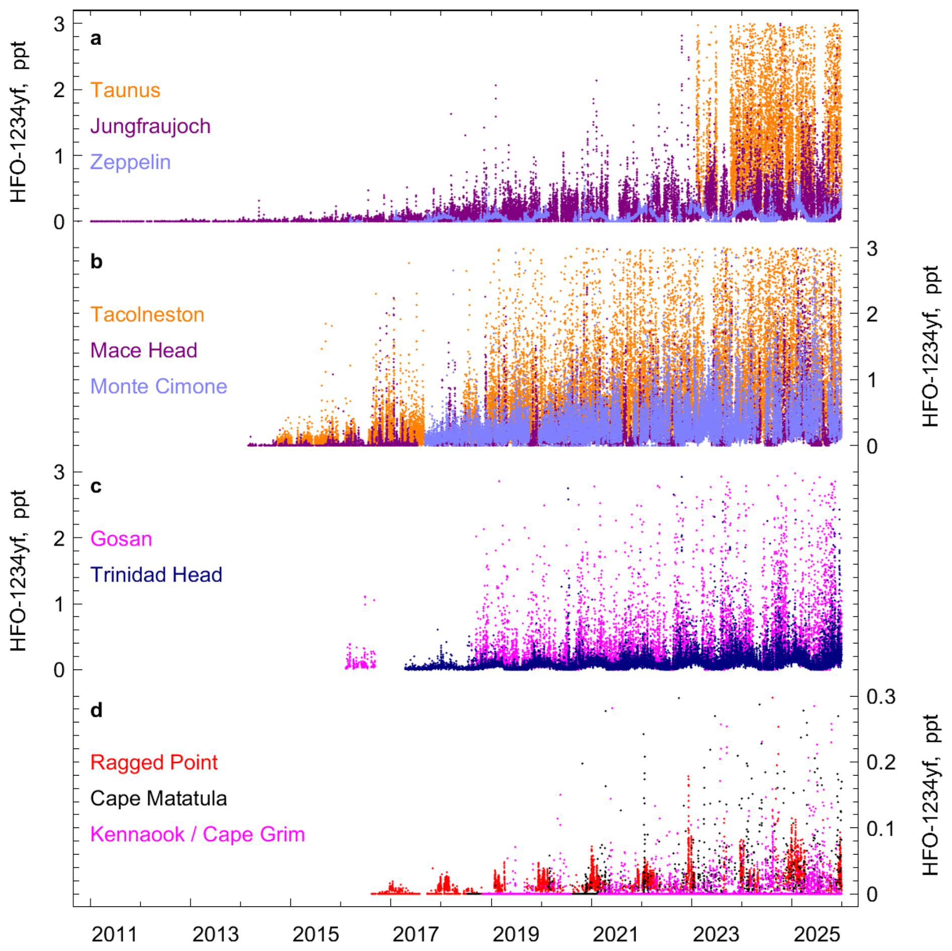
Figure 2 In situ observations of HFO-1234yf (CF₃CF=CH₂) from AGAGE stations. The records are separated into four subpanels for better visualization. (a) Taunus (Germany), Jungfraujoch (Switzerland), Zeppelin (Spitsbergen). (b) Tacolneston (UK), Mace Head (Ireland), Monte Cimone (Italy). (c) Gosan (Jeju Island, South Korea), Trinidad Head (California, USA). (d) Ragged Point (Barbados), Cape Matatula (American Samoa), and Kennaook/Cape Grim (Tasmania, Australia). Mole fractions larger than 3 ppt (0.3 ppt for panel d) are omitted from the plot.

2.5.6 ELRIS

ELRIS optimized emissions on a reduced-resolution grid that exhibits finer resolution in areas of large average SRR (usually close to the observational sites) and coarser resolution in areas with low SRR. Areas below a certain threshold SRR and ocean-only grid cells were excluded from the optimization, but treated as part of four remote regions. In addition to emissions, background concentrations at the domain interfaces were optimized in ELRIS following the InTEM approach (Manning et al., 2021) with the difference of employing temporally variable mole fractions at the 11 domain interfaces that were varied monthly. A priori background mole fractions are constructed from a Robust Extraction of Baseline Signal (REBS) fit (Ruckstuhl et al., 2012) to the observations of the coastal site Mace Head that often represents the inflow into Europe. To avoid negative a posteriori emissions ELRIS uses the approach suggested by Thacker (2007), which iteratively forces grid cells with negative a posteriori emissions to zero. A priori emission uncertainties were set such that uncertainties for each country in the inversion domain were 100 % of the emissions (1σ level). Covariance between different a priori emissions were represented by an exponentially decaying influence with distance and a length scale of 500 km. The resulting total a priori uncertainty for NW Europe was approximately 50 %.

The transport model uncertainty is derived iteratively from the residuals of the simulated minus observed model fractions and contains a constant contribution and a contribution linearly growing with the simulated a priori mole fractions (Henne et al., 2016). It is scaled such that the a posteriori chi-square index (Berchet et al., 2013) becomes unity. The background uncertainty is set to that estimated by the REBS fit. Four iterations of the inversion are used to derive the final model-data-mismatch uncertainty.

For the non-mountain sites (MHD and TAC), observations were filtered using the same criteria as RHIME. For the mountain sites (JFJ and CMN) ELRIS applied a filter to exclude observations during times when the model boundary layer height was within 50 m of the particle release height.

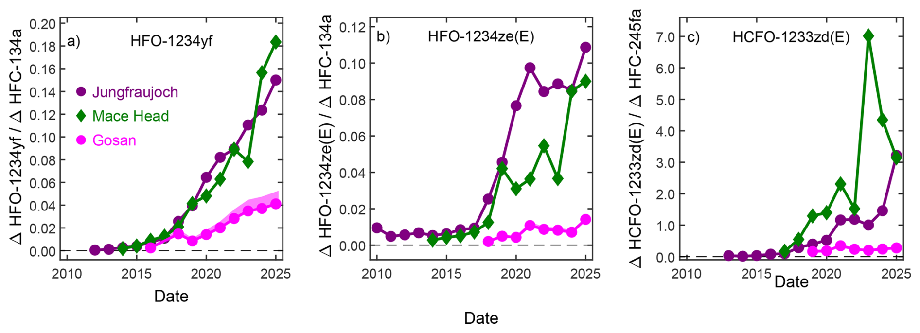
Figure 3 Ratios of pollution magnitudes (above baseline, Δ) of HFO-1234yf (a) and HFO-1234ze(E) (b) to HFC-134a and of HCFO-1233zd(E) to HFC-245fa (c) at Jungfraujoch, Mace Head, and Gosan. The sources of the substances are assumed to be co-located for each site. An approximated estimate for a decay correction is applied to the haloolefins for the Gosan measurements by correcting the yearly means for an average conservative transport time of four days and the yearly averaged lifetimes (Table S1 in the Supplement). This correction is shown as a shaded band and only large enough to be visible for HFO-1234yf. The elevated ratios found at Jungfraujoch and Mace Head compared to Gosan suggest an earlier replacement of HFC-134a and HFC-245fa by the HFOs and HCFO-1233zd(E), respectively, in Europe compared to the source region covered by Gosan.

3 Results and Discussion

3.1 Atmospheric Observations

Initially, the three haloolefins were only measured at Jungfraujoch (Vollmer et al., 2015), whereas measurements at most other stations began around 2015 (Figs. 2–5). However for many stations, the first few years of measurements were discarded because quaternary working and/or tertiary standards were not yet spiked with these species (see Methods), preventing accurately-calibrated air measurements. Fully calibrated measurements became available in 2014 from Mace Head and Ragged Point (for HFO-1234ze(E)) and starting in 2016–2018 from most other stations (Table 1). In general there is large variability in the observed mole fractions, depending on the proximity of the station to source regions and due to the short and seasonally varying lifetimes.

3.1.1 HFO-1234yf and HFO-1234ze(E)

At most sites, HFO-1234yf and HFO-1234ze(E) show a significant fraction of the observations below the detection limits in summer due to the much shorter atmospheric lifetime during this season (Figs. 2, 4 and Sect. S1, Figs. S1 and S2). However, Northern Hemisphere (NH) sites with closer proximity to the pollution regions exhibit a large fraction of observations above detection limits. Large pollution events are recorded at the Tacolneston and Taunus stations, with HFO-1234yf frequently reaching 2–10 ppt (picomol mol⁻¹). Increased use of the HFOs in the NH is also reflected in the Mace Head record. There, mole fractions of the HFOs were often below the detection limit in all seasons during the early observational years (2014–2018). In recent years, mole fractions of HFO-1234yf and HFO-1234ze(E) during winter months were mostly above the detection limit. Pollution events were very small and infrequent in 2014/2015, but have become more frequent and with larger magnitudes (several ppt) after that. Also, these compounds are detected in air masses that have pronounced narrow footprints over the Atlantic and the American continent, and are likely to result from emissions in North America.

At the southern hemisphere sites Cape Matatula and Kennaook/Cape Grim, the majority of the measurements show undetectable HFOs. Nearly all detectable HFOs at Kennaook/Cape Grim are associated with air mass transport from the Melbourne region, ∼ 330 km north of the site. Even though the pollution events have become more frequent at these two sites, their magnitudes have never exceeded 1 ppt (HFO-1234yf) and 0.5 ppt (HFO-1234ze(E)).

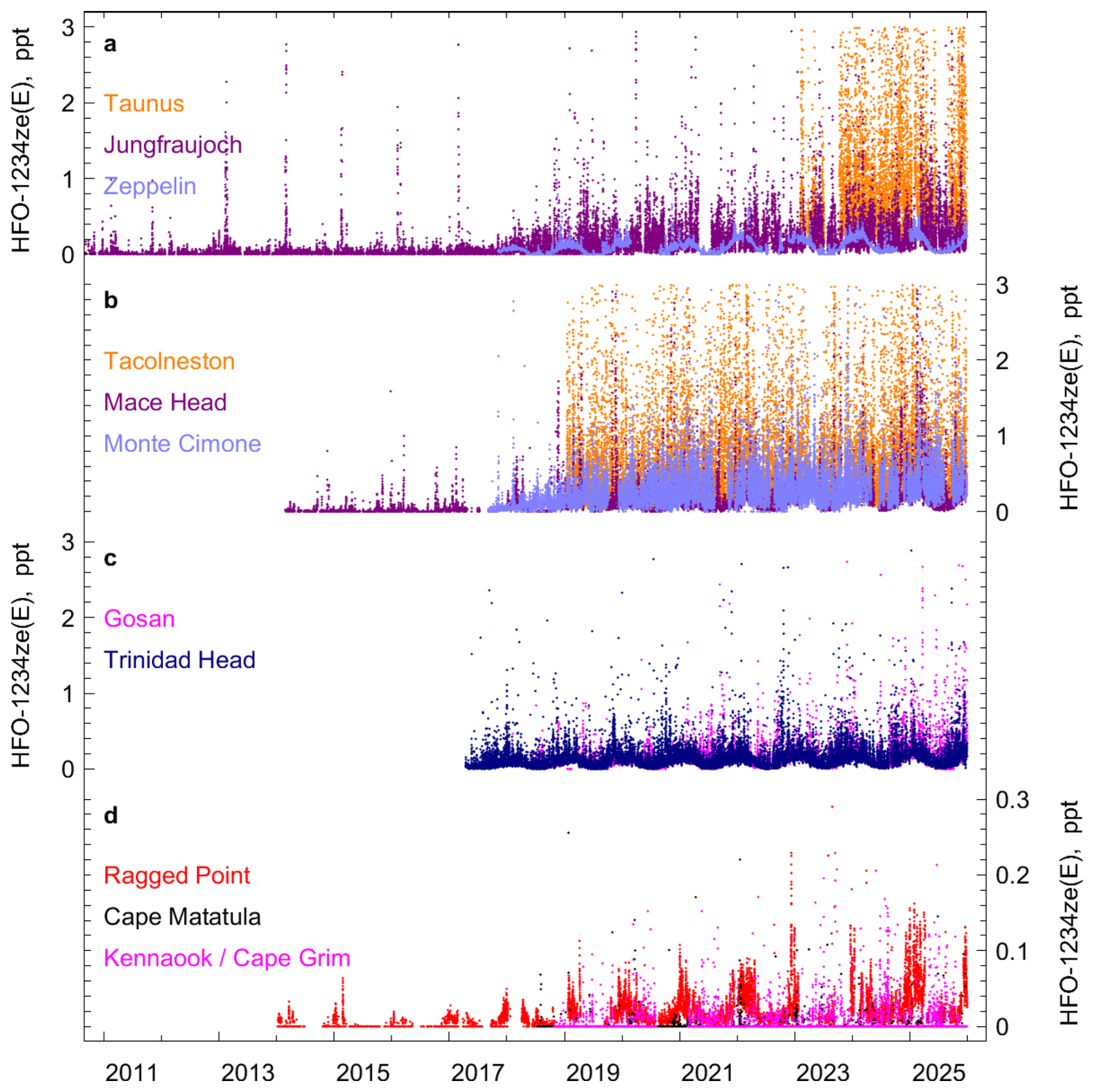
Figure 4 In situ observations of HFO-1234ze(E) ( trans-CF₃CH=CHF) from AGAGE stations. The records are separated into four subpanels for better visualization. (a) Taunus (Germany), Jungfraujoch (Switzerland), Zeppelin (Spitsbergen, Norway). (b) Tacolneston (UK), Mace Head (Ireland), Monte Cimone (Italy). (c) Gosan (Jeju Island, South Korea), Trinidad Head (California, USA). (d) Ragged Point (Barbados), Cape Matatula (American Samoa), and Kennaook/Cape Grim (Tasmania, Australia). Mole fractions larger than 3 ppt (0.3 ppt for panel d) are omitted from the plot.

Frequent pollution events are recorded at Gosan, suggesting that HFO-1234yf and HFO-1234ze(E) are also used within the footprint region of this station. Previous studies for other halocarbons (e.g. HFCs; Choi et al., 2024) measured at Gosan have shown large enhancements relative to background, which strongly exceed those at other stations, e.g., Mace Head. This is different for the two HFOs (and also for HCFO-1233zd(E)) where we find pollution magnitudes at Gosan which are of similar size compared to Mace Head. These observations suggest a delayed replacement of HFC-134a by the HFOs in this SE Asian region compared to Europe. This is illustrated in Fig. 3a and b where we compare the pollution magnitudes of the two HFOs in relation to those for HFC-134a. We determine linear fits for the above-baseline pollution events of HFO-1234yf (ΔHFO-1234yf) against those of HFC-134a (ΔHFC-134a) for each year of observations using linear regression based on least-square methods (Fig. S4) and show these as timeseries in Fig. 3a and b. The linear fit slopes (ratios) increase strongly over the observational period, and are higher for Jungfraujoch and Mace Head compared to Gosan. This is indicative of a faster transition from HFC-134a to HFO-1234yf and HFO-1234ze(E) for Europe compared to the footprint regions of Gosan, in line with the stringent HFC phase-out regulations in Europe.

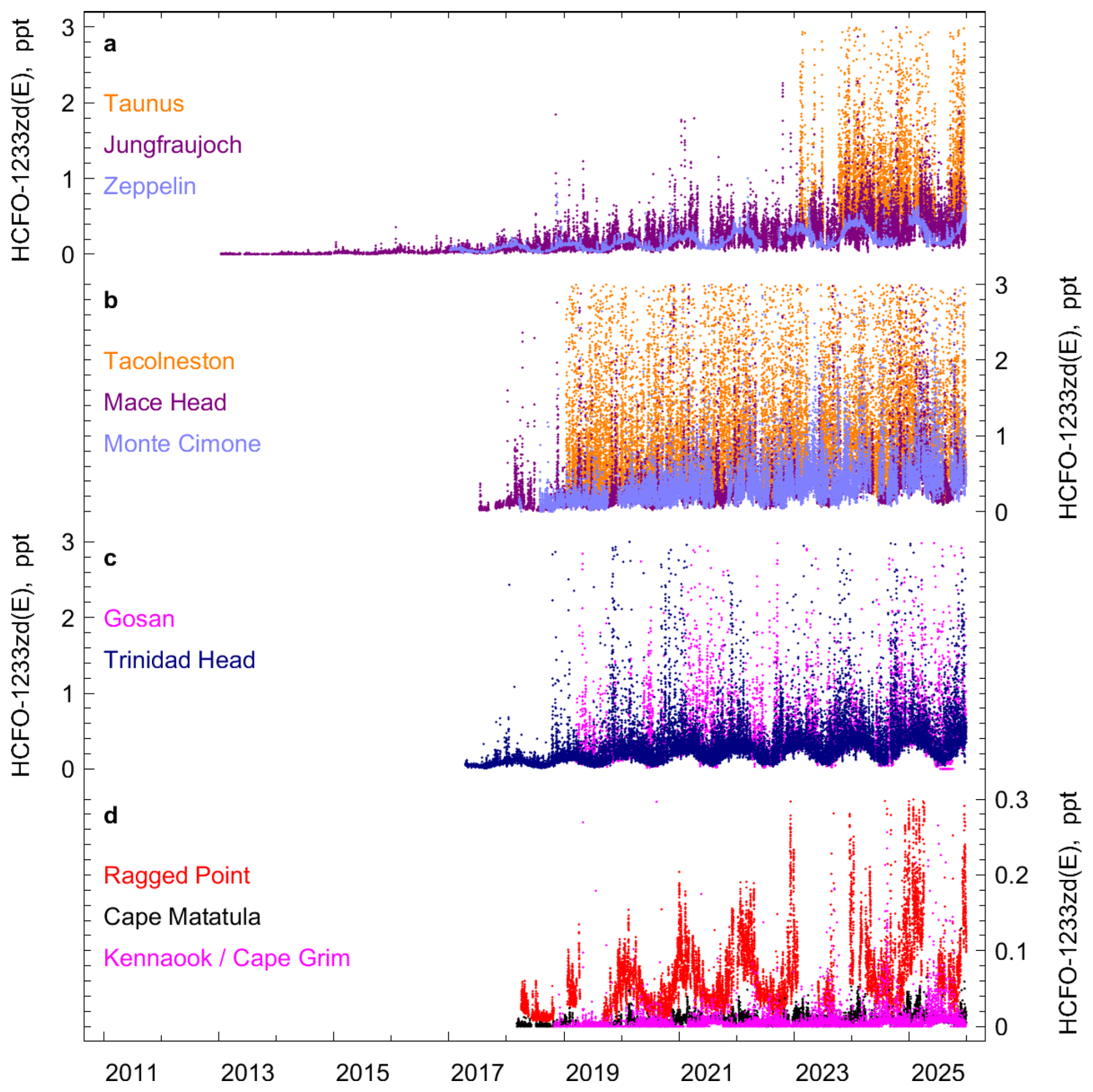
Figure 5 In situ observations of HCFO-1233zd(E) (trans-CF₃CH=CHCl) from AGAGE stations. The records are separated into four subpanels for better visualization. (a) Taunus (Germany), Jungfraujoch (Switzerland), Zeppelin (Spitsbergen, Norway). (b) Tacolneston (UK), Mace Head (Ireland), Monte Cimone (Italy). (c) Gosan (Jeju Island, South Korea), Trinidad Head (California, USA). (d) Ragged Point (Barbados), Cape Matatula (American Samoa), and Kennaook/Cape Grim (Tasmania, Australia). Mole fractions larger than 3 ppt (0.3 ppt for panel d) are omitted from the plot.

3.1.2 HCFO-1233zd(E)

For HCFO-1233zd(E), more measurements are at detectable mole fraction levels compared to the two HFOs (Fig. 5). While for the earlier records this was mainly due to lower analytical detection limits, in more recent years this is attributed to the longer lifetime (roughly doubled compared to the two HFOs). Early Jungfraujoch observations showed HCFO-1233zd(E) mole fractions that were about one order of magnitude smaller compared to the HFOs, and much fewer pollution events in the footprints of the station. Since 2016 almost all observations of HCFO-1233zd(E) in NH air masses reveal detectable mole fractions. The only exception is the tropical remote Ragged Point station where some NH air masses contained undetectable HCFO-1233zd(E) up to 2018 but not in more recent years. HCFO-1233zd(E) at Gosan is also above detection limits except for short periods with pronounced SH advection. In general, the seasonal apex (maximum) background HCFO-1233zd(E) mole fractions have exceeded those of the HFOs in the NH. The combination of fewer emissions and longer lifetime leads to a much more pronounced seasonality in the measurement records, and fewer pollution episodes, most clearly seen at Zeppelin. There the apex of the background mole fractions has increased from 0.07 ppt in early 2017 to 0.4 ppt at the end of 2023. Only the two SH sites at Samoa and Kennaook/Cape Grim exhibit a significant fraction of undetectable HCFO-1233zd(E) in their records. However, during the austral summer 2021/2022 all measurement at the two sites contained detectable HCFO-1233zd(E). First clear detection of HCFO-1233zd(E) at Antarctic King Sejong started in austral winter 2021 (see Sect. S3).

At Gosan, HCFO-1233zd(E) pollution events are similar in magnitude to Mace Head. To illustrate the delayed replacement of HFCs by HFCO-1233zd(E) we proceed in analogy to the two HFOs but because foam blowing is the main application for HCFO-1233zd(E), we here compare to HFC-245fa (Fig. 3c). Like for the two HFOs, the pollution ratios at Gosan compared to Mace Head and Jungfraujoch, (ΔHCFO-1233zd(E)/ΔHFC-245fa) suggest a delayed replacement of HFC-245fa by HCFO-1233zd(E) in the footprint region of Gosan (Figs. 3c, S5).

3.2 Northwest European (NW) Emissions

Observation-based emissions for the three haloolefins are determined using the three model frameworks: InTEM, ELRIS and RHIME. These 10-year emission timeseries (7-year for HCFO-1233zd(E)) are shown in Fig. 6 for the individual frameworks and for their multi-model mean. InTEM emission estimates for HFC-134a are also shown; these are taken from the model runs used in the 2025 UK National Inventory Document (NID) submitted to the United Nations Framework Convention on Climate Change (UNFCCC) (https://unfccc.int/, last access: 12 May 2026). Given that European measurements of the haloolefins started already at the time of the market phase-in of these chemicals, we are able to derive their entire emission histories. Consequently, the emissions of HFO-1234yf (Fig. 6b) and HFO-1234ze(E) (Fig. 6c) are virtually absent at the beginning of the investigated period in 2014. Here, we only present results from our base inversions (lifetime-aware source sensitivities, population-based a priori distribution). Additional sensitivity tests (assuming inert tracer and uniform/flat a priori) are given in the Sect. S5 and Fig. S9.For HFO-1234yf, NW European emissions increased from 0.03 [0.02–0.06] Gg yr⁻¹ in 2014 to 1.50 [1.23–1.74] Gg yr⁻¹ in 2023. All uncertainties are given as the range bounded by the 15.9 percentile of the lowest model and the 84.1 percentile of the highest model. This increase is likely dominated by its phase-in in MAC, in replacement of HFC-134a. Over the same time period, HFC-134a emissions have not increased, supporting this interpretation. The relatively linear increase in HFO-1234yf emissions suggests that the transition in MAC was gradual. This is in line with a gradual phase-in of HFO-1234yf into the European vehicle fleet as the EU MAC regulation (European Parliament and Council, 2006), which came into effect in January 2017, applies only to new vehicles.

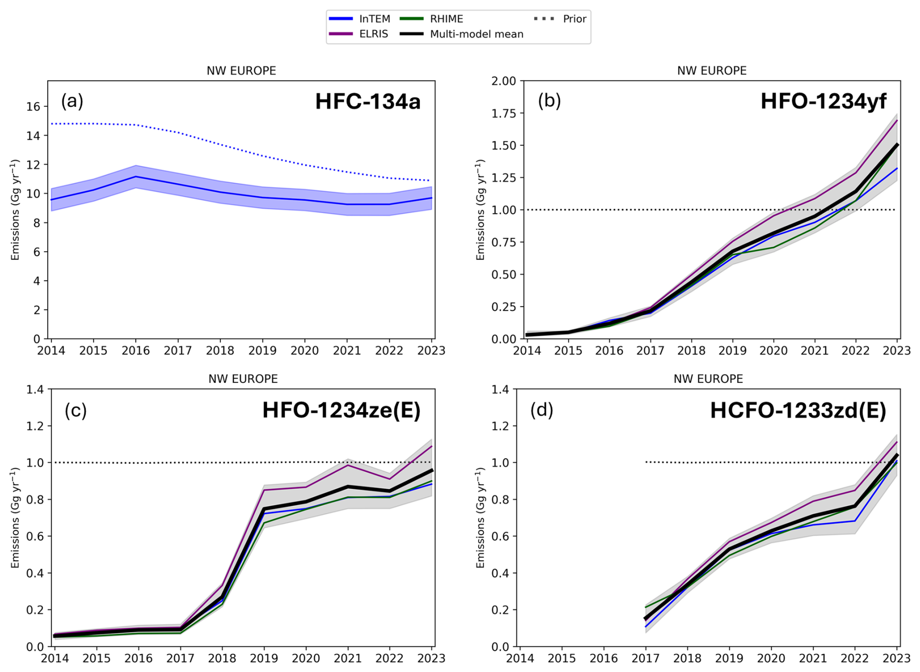
Figure 6 Emissions of HFC-134a, HFO-1234yf, HFO-1234ze(E), and HCFO-1233zd(E) from Northwest (NW) Europe (Belgium, Germany, France, UK, Ireland, Luxembourg and the Netherlands). Emissions are shown for the three model approaches InTEM, ELRIS, and RHIME and for their multi-model mean. The uncertainty range shown in grey is bounded by the 15.9 percentile of the lowest model and the 84.1 percentile of the highest model. Prior emissions for the three haloolefins are set uniformly at 1 Gg yr⁻¹. Emissions are increasing monotonically and strongly for the haloolefins during the observational periods. For HFO-1234ze(E), the large increase in the emissions in 2018 and 2019 is a robust feature and also seen in the countries with the largest emissions (France, Germany, and UK, see Supplement). Emissions of HFC-134a are from InTEM only, 3-year smoothed and are taken from the model runs used in the 2025 UK NID submitted to the UNFCCC (with a range representing the 1σ posterior uncertainty).

Using a population-based extrapolation from the NW Europe countries (254 million people in 2023, EUROSTAT, 2025b) to the EU27+ (27 EU countries plus the UK, Switzerland, and Norway, 530 million people in 2023), results in 3.1 [2.6–3.6] Gg for 2023 for EU27+. Alternatively, almost identical emissions (3.2 [2.6–3.7] Gg) are obtained if we upscale emissions based on number of passenger cars (in 2023, NW Europe 139 million vs 296 million in the EU27+, EUROSTAT, 2025a). In both cases, the uncertainty ranges only relate to the uncertainty in NW European emissions and do not account for uncertainty using this upscaling approach.

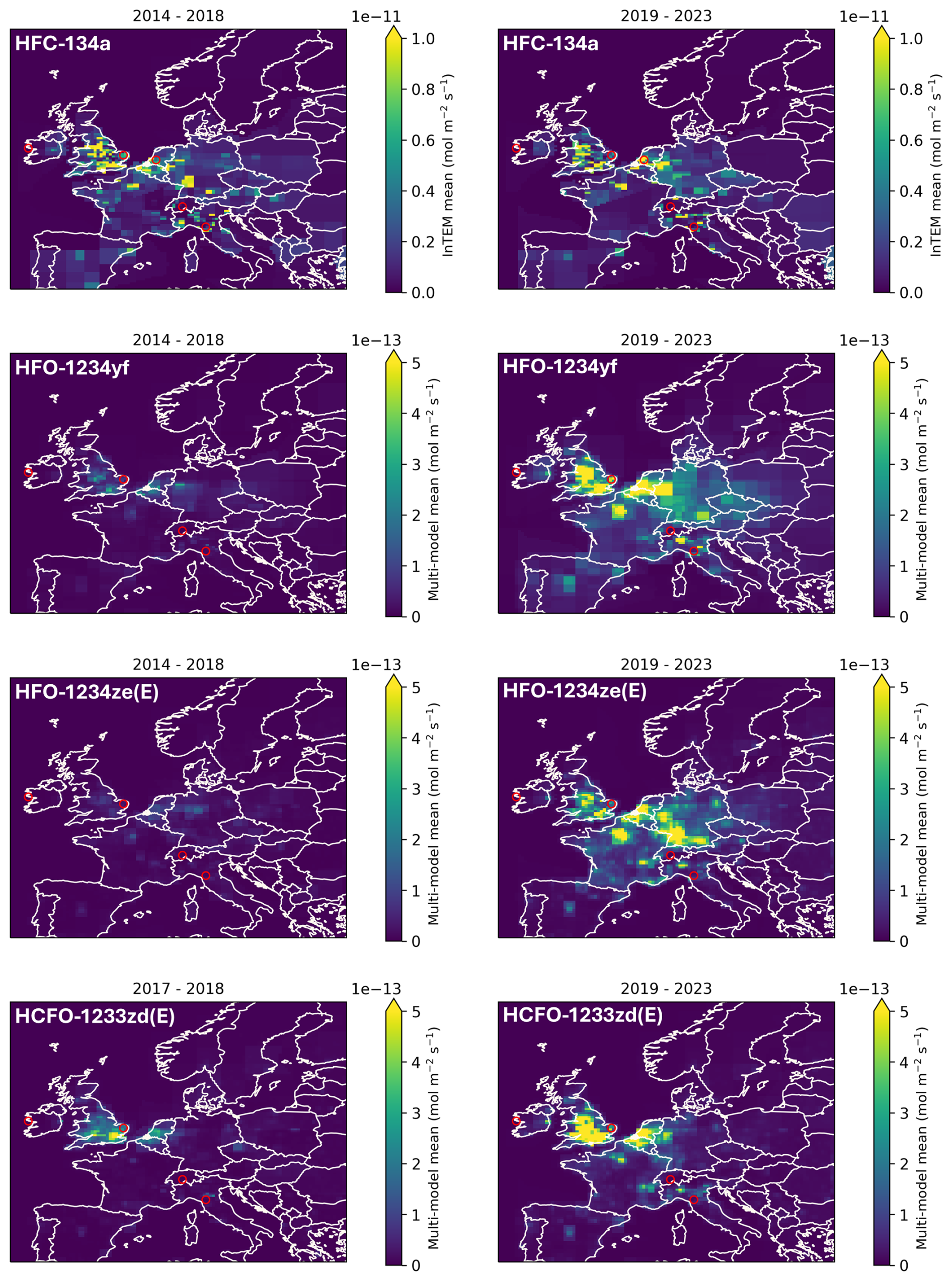
Figure 7 Emissive flux maps for Northwest (NW) European for HFC-134a, HFO-1234yf, HFO-1234ze(E) and HCFO-1233zd(E) for 2014–2018 (2017–2018 for HCFO-1233zd(E)) in the left panels and for 2019–2023 in the right panels. The scale for HFC-134a is two orders of magnitude larger than those for the haloolefins. Red circles denote measurement sites and are, from west to east, Mace Head (Ireland), Tacolneston (UK), Cabauw (NL, for HFC-134a from flask samples only), Jungfraujoch (Switzerland), and Monte Cimone (Italy).

In contrast to the linear increase of the HFO-1234yf emissions, that of HFO-1234ze(E) (Fig 6c) shows two inflection points. Emissions initially stayed relatively low (2014–2017), followed by a rapid increase, before slowing down again and reaching 0.96 [0.82–1.13] Gg yr⁻¹ in 2023 (population-based extrapolation to EU27+ results in 2.0 [1.7–2.3] Gg yr⁻¹). This pattern is robust against selective onsets of some measurement sites as was tested by dropping selective sites. It is also seen in the four largest emission regions (France, Germany, UK, and Benelux, see Supplement. The reasons for this rapid onset are unclear. One could be the EU ban on the use of HFC-134a in technical aerosols, starting in January 2018. This could have boosted the use of HFO-1234ze(E), even though other alternatives (HFC-152a, hydrocarbons and dimethylether) also became available. Since this application results in immediate and complete emissions, such a replacement could explain the derived rapid emission increase. If the increase of ∼ 0.7 Gg HFO-1234ze(E) over 2018–2019 resulted in a corresponding decrease of HFC-134a emissions, it would be difficult to detect within the overall large HFC-134a emissions. Another potential regulation causing the rapid growth in HFO-1234ze(E) emissions is the EU 2020 ban on HFCs in foam, which may have been met with an early change to HFO-1234ze(E). 2018 is also the start of the Kigali Amendment HFC phase-down which may have caused a strong increase in the use of HFO-1234ze(E).

HCFO-1233zd(E) emissions (derived from 2017 onward) increased steadily (similar to HFO-1234yf), reaching 1.04 [0.93–1.15] Gg in 2023. A population-based extrapolation to EU27+ results in 2.2 [1.9–2.4] Gg in 2023.

In Fig. 7 we show the geographical distributions of the changes in emission for NW Europe for 2014–2018 and 2019–2023. For HFC-134a the emission distribution is comparably invariant over the two periods, while emission centers for HFO-1234yf and HFO-1234ze(E) appear only in the second period. For HFO-1234yf, the geographical distribution of the emissions for 2019–2023 strongly resembles that for HFC-134a and suggests that the use of HFO-1234yf is in similar applications to that for HFC-134a (most likely MAC). HFO-1234ze(E) also shows a similar distribution for 2019–2023, but for HCFO-1233zd(E) emissions centers are strongly biased towards the UK and Benelux countries and appear already in the 2017–2018 period. This suggests that the introduction of this chemical occurred differently in individual European countries. Reasons for this may be regulatory (HCFO-1233zd(E) contains a chlorine and permissions for use may be handled differently) or that its use in specific applications (e.g., foam blowing) was delayed in some countries.

4 Conclusions

We report on the first large-scale AGAGE network observations of HFO-1234yf, HFO-1234ze(E), and HCFO-1233zd(E), three recently marketed haloolefins used as replacements for HFCs. We estimate emissions for specific regions and countries in NW Europe and find increasing emissions to 1.50 [1.23–1.74], 0.96 [0.82–1.13], and 1.04 [0.93–1.15] Gg by 2023, for HFO-1234yf, HFO-1234ze(E), and HCFO-1233zd(E), respectively. We conclude this as evidence of an ongoing transition away from HFCs, which are phased-down under the F-gas regulation and the Kigali Amendment of the Montreal Protocol. The support for this conclusion comes from stagnant emissions of HFC-134a (Manning et al., 2021), which is one of the main HFCs targeted for phase down. Our results allow for comparison with inventory emissions as soon as these are publicly available. Because of the spatial sparsity of the observations in the AGAGE network, we are currently unable to conduct regional estimates other than for Northwest Europe. Emission estimates on a global level using box models (e.g. AGAGE 12-box model Cunnold et al., 1983; Rigby et al., 2013; Western et al., 2025) are inappropriate given their coarseness and the short atmospheric lifetimes of the haloolefins. However, more sophistical global models such as GEOS-Chem (e.g. Bey et al., 2001; Tewari et al., 2025; The International GEOS-Chem User Community, 2023) or STOCHEM (e.g. Holland et al., 2021), that include detailed chemistry could potentially be applied to gain a more complete picture of global emissions. This could be complemented by further regional studies of Asian regions, which should become possible as more measurements become available from there. The present data base can also support studies of atmospheric decay products e.g., TFA deposition, which are necessary to assess the environmental impact of the haloolefins. Since the atmospheric chemistry and environmental effects of the haloolefins are still poorly understood, it is crucial to further our understanding of the atmospheric abundances and emissions of these substances.