Measurement report: Insights into the high temporal variability of atmospheric carbon dioxide (CO₂) at a suburban station in the Indo-Gangetic Plain

The unusual weather patterns and large anthropogenic emissions over the Indo-Gangetic Plain (IGP) make it a significant hotspot of greenhouse gases like carbon dioxide (CO₂). Given the significance of the IGP and highly populated Delhi National Capital Region (Delhi-NCR), a GHG observatory was established at a suburban monitoring station in Sonipat, Haryana (28.95° N, 77.10° E; 228 m a.s.l.), about 45 km north of the Delhi state boundary. Using a laser-based cavity ring-down spectroscopy (CRDS) technique, we measured CO₂ mole fraction from February 2023 to January 2025. An annual average CO₂ mole fraction of 440.8 ± 19.7 parts per million (ppm) was recorded in 2024, which includes a strong seasonal variability, ranging from 422.6 ± 23.3 ppm during the monsoon (June–September) to 456.4 ± 30.8 ppm in post-monsoon (October–November). A strong CO₂ diurnal amplitude of 29 ppm in May and 63 ppm in October was observed mainly due to seasonal changes in boundary layer mixing (faster in May than October) and biospheric activity (weaker in May than October). Further investigation of the drivers of strong seasonal and diurnal CO₂ variability over IGP revealed a strong contrast to other global monitoring stations in the same latitude band. A strong correlation between CO₂ and methane (CH₄) indicated a co-located emission source, while the strong positive correlation between CO₂ and carbon monoxide (CO) during post-monsoon emerges due to emissions from biomass burning. We demonstrated that the high temporal CO₂ variability in the IGP region is driven by the complex interplay of local anthropogenic and biomass burning emissions, biospheric fluxes, and prevailing meteorology.

1 Introduction

Carbon dioxide (CO₂) is the major greenhouse gas (GHG) contributing to climate change and global warming (IPCC, 2021; Fawzy et al., 2020). Due to the long lifetime and high radiative forcing potential, CO₂ can have a significant impact on global and regional climate (Wang et al., 2010). The atmospheric CO₂ mole fraction has increased from 278 parts per million (ppm) in the pre-industrial period to 427 ppm in 2025 (NOAA, https://gml.noaa.gov, last access: 20 July 2025; Wigley, 1983). This rapid increase in the atmospheric fraction of CO₂ is primarily due to the combustion of fossil fuels, cement manufacture, deforestation, and other industrial processes (Stocker et al., 2013; Huang et al., 2016; Yoro and Daramola, 2020). A comprehensive understanding of the sources and sinks of CO₂ is critical for developing national policies to mitigate climate change impacts.

India is the third-highest CO₂-emitting nation (8 % of total global CO₂) in the last decade, as reported by the Global Carbon Project (GCP) (Friedlingstein et al., 2025; Le Quéré et al., 2018). In particular, the Indo-Gangetic Plain (IGP) region is one of the hotspots of atmospheric CO₂ mole fraction, primarily due to large fossil fuel emissions and adverse meteorology (Halder et al., 2021; Krishnapriya et al., 2025; Kuttippurath et al., 2022). Over the past few decades, the IGP region has witnessed rapid urbanisation, industrialisation, and agricultural intensification, leading to significant changes in land-use patterns and GHG emissions (Yoro and Daramola, 2020). Mitigation of anthropogenic CO₂ emissions in the highly populated IGP region is crucial to reducing the build-up of atmospheric CO₂ mole fractions. Gaining a better understanding of the magnitude of CO₂ sources and sinks and the local drivers of CO₂ temporal variability over the IGP region is therefore important.

Continuous monitoring of ground-based CO₂ is of utmost importance for inverse modelling approaches to understand local-to-regional-scale sources and sinks of CO₂. Although GHG mole fractions have been monitored worldwide for decades, GHG monitoring stations in India are limited (Kunchala et al., 2025; Chakraborty et al., 2020; Kumar et al., 2021; Patra et al., 2013; Tiwari et al., 2013). The Cape Rama (15.08° N, 73.83° E) station, situated on India's southwest coast, was the first Indian monitoring station to track CO₂ mole fraction from 1993 to 2002 (Bhattacharya et al., 2009; Patra et al., 2011; Rayner et al., 2008). Recently, several monitoring stations have been established over different parts of India to measure the GHGs (Chandra et al., 2016; Jain et al., 2021; Mahesh et al., 2015; Metya et al., 2021; Nomura et al., 2021; Pathakoti et al., 2023; Sreenivas et al., 2016; Thilakan et al., 2024; Tiwari et al., 2014). Studies have also been conducted using aircraft-based measurements (Niwa et al., 2012; Patra et al., 2011; Schuck et al., 2012; Zhang et al., 2007) and satellite data products (Das et al., 2023; Kunchala et al., 2022; Nalini et al., 2019; Philip et al., 2022; Xiong et al., 2009). The incorporation of regional in situ and aircraft-based measurements, along with satellite columnar CO₂ retrievals, reduced uncertainties in top-down CO₂ flux estimates (Huang et al., 2008; Niwa et al., 2012; Zhang et al., 2014).

To comprehensively understand temporal CO₂ variability and its drivers in the western IGP region, we have conducted atmospheric CO₂ mole fraction measurements at Sonipat, a suburban station in the IGP region upwind of Delhi. The continuous measurements from February 2023 to January 2025 were conducted using laser-based cavity ring-down spectroscopy. Here, we investigate the novel characteristics of the seasonal and diurnal variability of atmospheric CO₂ mole fraction at Sonipat. We then identify the key drivers of the observed temporal CO₂ variability in the region.

2 Materials and methods

2.1 Monitoring station

The measurements in this study were carried out at the Indian Institute of Technology Delhi (IIT Delhi) Centre for Atmospheric Sciences (CAS) – Atmospheric Observatory situated at Sonipat campus (28.95° N, 77.10° E, 228 m a.s.l.). Sonipat is an upwind suburban region of the Delhi-NCR, situated in the northern Indian state of Haryana, approximately 45 km north of Delhi. The monitoring station is surrounded by agricultural fields, a National Highway, and academic institutions (Rathore et al., 2025). Figure 1 shows the location map of the monitoring station. The climatic conditions over this site are similar to Delhi which has sweltering summers (March–May), damp or moist monsoons (June–September), and extreme winters. Similar to Delhi, this region also has frequent haze and smog with low visibility during winter (December–February) and post-monsoon (October–November) seasons. During the post-monsoon season, Sonipat experiences large transport of pollutants from the North-West direction. In addition to the pollutant transport, several local emission sources exist in the region, such as small industries, vehicular sources, and local biomass burning affecting short-lived air pollutants (Rathore et al., 2025).

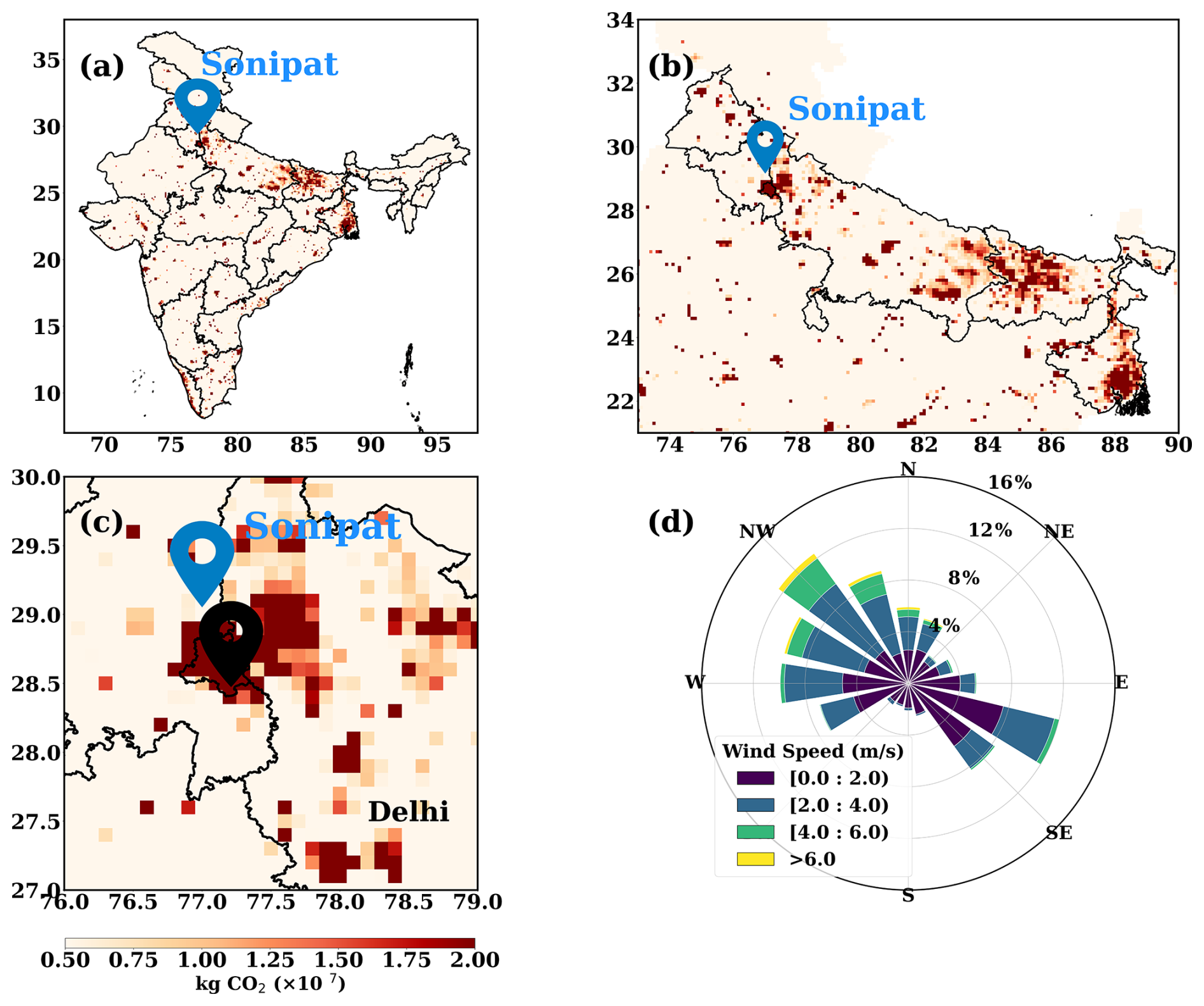
Figure 1 Anthropogenic CO₂ emissions over (a) India (b) IGP and (c) Sonipat/Delhi derived from the EDGAR emission inventory for 2021. (d) Annually averaged wind patterns over Sonipat for February 2023–January 2024.

2.2 Local measurements

2.2.1 GHG measurements

This study utilised the PICARRO G2301 GHG analyser to measure major atmospheric GHG mole fractions. The PICARRO analyser employs the Cavity Ring-Down Spectroscopy (CRDS) technique at 0.5 Hz to measure CO₂ mole fraction. The CRDS technique utilises the ring-down time of light intensity within the cavity to determine the mole fraction of CO₂, a method fundamentally different from other measurement techniques such as Non-dispersive Infrared Spectroscopy (NDIR) and Fourier Transform Infrared Spectroscopy (FTIR). The long sample interaction path length (approximately 20 km) is a characteristic of CRDS, which enhances sensitivity compared to conventional techniques based on light-intensity absorption. The cavity pressure operates at a very low pressure of 140 Torr. This isolates a single spectral feature with a resolution of 0.0003 cm⁻¹, ensuring a linear relationship between peak height or area and mole fraction. The CRDS provides precise, highly sensitive measurements of gases in ambient air with a temporal resolution of 5 s. The technique has been well validated for measuring atmospheric CO, CO₂, and CH₄ mole fractions globally and at some Indian monitoring stations (Chandra et al., 2016; Chen et al., 2013; Jain et al., 2021).

The standard cavity temperature of 45 °C (throughout the measurement period) ensures the necessary etalon mechanical stability of the measurement cavity. The sample air was taken from the top of the building and above the tree canopy (5 m above the instrument housing) through a Teflon (PTFE) tube with an inner diameter of 3 mm using an external vacuum pump with ∼400 sccm flow rate (residence time ∼5.9 s). The air intake height is about 248 m.

The Sonipat station, lying on the upwind side of Delhi, is a suburban station with relatively cleaner air compared to the urban city centre. However, Sonipat cannot be considered a pristine site due to the impact of local emissions from nearby industries and national highways. We adopted (1) the fifth percentile of the daily data to characterise background mole fraction at the site (Ammoura et al., 2014; Chandra et al., 2016; Jain et al., 2021), and (2) the adaptive diurnal minimum variation selection (ADVS) method that considers the diurnal minimum value as the daily background value (Apadula et al., 2019; Yuan et al., 2018). In this study, the comparison between the fifth percentile and the ADVS methods showed similar CO₂ background values (see Fig. S1 in the Supplement), and the ADVS method was used for further analysis. The excess CO₂ mole fractions were then estimated by subtracting the hourly averaged values of CO₂ from the background mole fraction.

The measurements of the atmospheric CH₄ mole fraction were also conducted with the PICARRO G2301 GHG analyser. The GHG analyser employs the CRDS at 0.5 Hz to measure CH₄ mole fraction. The mole fractions of CH₄ were determined using the ring-down time of light intensity, similar to CO₂ mole fractions. Calibration was performed following the guidelines of the National Oceanic and Atmospheric Administration Earth System Research Laboratories (NOAA-ESRL, 2020) and the Integrated Carbon Observation System (ICOS) protocol (ICOS RI, 2020), using NOAA standard calibration cylinders. Further details of the calibration process are provided in Sect. S1 in the Supplement.

2.2.2 Trace gas measurements

In addition to the measurements of CO₂ and CH₄, we also utilised the measurements of trace gases to establish the species interrelationships and to identify drivers of GHG sources. We used a compact air-quality measurement instrument with gas sensors (CUPI-G) to continuously measure air pollutants, including fine particulate matter (PM_2.5), nitric oxide (NO), nitrogen dioxide (NO₂), and carbon monoxide (CO). The sensors used in CUPI-G are a palm-sized optical PM_2.5 sensor developed by Panasonic, a CO-B4 Carbon Monoxide Sensor, and an NO-B4 Nitric Oxide Sensor developed by Alphasense. The sensitivity of the PM_2.5 and CO sensors was evaluated in Nagasaki, Japan, through intercomparisons with reference-grade instruments employing a beta attenuation monitor (BAM) for PM_2.5 and non-dispersive infrared (NDIR) spectroscopy for CO measurements (Fig. S1). The estimated unit-to-unit variability was 29 % for PM_2.5 sensors and 21 % for CO sensors. Further details on the sensor specifications and the calibration methodology are described in Mangaraj et al. (2025).

2.2.3 Local meteorology measurements

A Vaisala Ceilometer lidar CL61 provides real-time measurements of cloud base height (CBH) for up to five layers, along with depolarisation measurements, under all weather conditions. To determine the Planetary boundary layer height (PBLH) from the range-corrected attenuated backscatter data, the gradient method (Summa et al., 2013) and the Wavelet Covariance Transform (WCT) method (Baars et al., 2008) were employed. Further details on PBLH calculations can be found in Rathore et al. (2025). An automatic weather station (AWS) by Geonica, installed on the I-Tech building rooftop, collected meteorological data at 5 min intervals. The data, including ambient temperature, relative humidity (RH), atmospheric pressure, wind speed and direction, precipitation, and incoming solar radiation, were retrieved using Datagraph-W4K 2.1.3.0 software and exported in CSV format. All sensors were meticulously calibrated and regularly cleaned to ensure accuracy and reliability.

2.3 Auxiliary data

2.3.1 ObsPack Data

To compare the seasonality of atmospheric CO₂ of Sonipat with other non-Indian sites in the same latitudinal band, we used selected sites from the obspack_co2_1_GLOBALVIEWplus_v10.1_2024-11-13 (Schuldt et al., 2024; Masarie et al., 2014). The data was averaged for five years from 2018 to 2022 for all stations except Boulder Atmospheric Observatory, Colorado, (2011–2016), to compare the seasonality over different locations across the globe.

2.3.2 Satellite CO₂ retrievals

Along with the ground-based in situ CO₂ measurements at the Sonipat monitoring station, we also used column average dry air CO₂ mole fraction (XCO₂) retrievals from the Orbiting Carbon Observatory-2 and 3 satellites (OCO-2 and OCO-3) (Crisp et al., 2017; Eldering et al., 2017). We used the bias-corrected OCO-2 v11.1r data product for the period from February 2023 to December 2024. The OCO-3 satellite provides XCO₂ data at a repeat cycle of 16 d with a spatial resolution of 1.60 km×2.25 km (nadir observation), which increases the swath area from ∼3.0 to ∼3.5 km². We used the bias-corrected OCO-3 v10.4r data product (Eldering et al., 2019; Srivastava et al., 2020) for the period from February 2023 to December 2024.

2.3.3 FluxSat GPP

To study the Gross Primary Production (GPP) fluxes over Sonipat, we used FluxSat v2.2 native GPP product computed at the spatio-temporal resolution of the MCD43C data set (daily at 0.05° spatial resolution) (Schaaf et al., 2002; Wang et al., 2018). FluxSat v2.2 has been derived from the MODerate resolution Imaging Spectroradiometer (MODIS) instruments on the NASA Terra and Aqua satellites using the collection 6.1 MCD43C Bidirectional Reflectance Distribution Function (BRDF)-Adjusted Reflectances (NBAR) (Joiner et al., 2018; Joiner and Yoshida, 2020; Schaaf and Wang, 2021). FluxSat v2.2 is “calibrated” using a set of the FLUXNET 2015 and OneFlux tier 1 (publicly released) eddy covariance (EC) data and has been compared with independent data (i.e., not used in the calibration) as validation. We used Global Gross Primary Production (GPP) estimates for 2023 in this study.

2.3.4 Ecosystem-proxy variables

We used two key ecosystem proxy variables to examine the carbon cycle dynamics at the Sonipat station and in the IGP region. The Normalised Difference Vegetation Index (NDVI) version 5 data from the Advanced Very High Resolution Radiometer (AVHRR) was used here (Vermote and NOAA CDR Program, 2018). The NDVI CDR summarises surface vegetation coverage activity based on measurements in the red and near-infrared spectral bands at daily intervals and at a spatial resolution of 0.05°×0.05°.

To understand the photosynthetic capacity of the regional ecosystem to assimilate atmospheric CO₂, we used Solar-Induced Chlorophyll Fluorescence (SIF) retrievals from the OCO-2 satellite (Frankenberg et al., 2014). The OCO-2 provides SIF data at a temporal resolution of 16 d and a spatial resolution of 1.35 km×2.25 km. The estimation of SIF relies on evaluating the in-filling of solar Fraunhofer lines at 757 and 770.1 nm surrounding the O₂ A-band (Frankenberg et al., 2014; Sun et al., 2018). We used bias-corrected SIF data from OCO-2 v11r and v11.2r SIF data products.

2.4 Models

2.4.1 JAMSTEC's MIROC version 4 atmospheric chemistry-transport model (MIROC4-ACTM)

We used the Model for Interdisciplinary Research on Climate version 4 (MIROC4), atmospheric general circulation model (AGCM)-based chemistry-transport model (MIROC4-ACTM; Patra et al., 2018), to simulate CO₂ mole fraction for this study. Simulations were performed at a horizontal resolution of T42 spectral truncations (∼2.8° latitude–longitude grid) with 67 vertical hybrid-pressure layers between the Earth's surface and 0.0128 hPa (∼80 km). CO₂ tracers were simulated corresponding to fossil fuel combustion (FFCO₂), land biosphere fluxes (LBCO₂), fire emissions (CO_2fire), and ocean exchanges (CO_2ocn) from different prior (bottom-up) emissions sets (Chandra et al., 2022). FFCO₂ was simulated using the gridded fossil fuel emission dataset (GridFED; Jones et al., 2021). LBCO₂ tracers were simulated using two sets of terrestrial biosphere fluxes from the Carnegie-Ames-Stanford Approach (CASA) biogeochemical model (Randerson et al., 1997) and Vegetation Integrative Simulator for Trace Gases (VISIT) (Ito, 2019).

2.4.2 CarbonTracker (CT) inverse model

To understand the temporal pattern of atmospheric CO₂ mole fraction over the study station and the IGP region, we used simulated CO₂ mole fraction from an inverse modelling framework CarbonTracker (CT) (Peters et al., 2005). Here, we used the CarbonTracker 2022 release (CT2022), which incorporated two-way nesting of the offline atmospheric tracer transport model TM5, supporting coarse-resolution global data and high-resolution regional data (Krol et al., 2005). The TM5 model in CT2022 was driven with meteorology from the ERA-interim reanalysis provided by the European Center for Medium-Range Weather Forecasts (ECMWF). The CT2022 inverse model simulated atmospheric CO₂ mole fraction by correcting the prior specifications of CO₂ sources and sinks in the model by assimilating global in situ observations. In this study, we used the CT2022-simulated CO₂ mole fraction from February 2023 to October 2023.

2.4.3 GEOS-Chem inverse model

To study the seasonality of the fluxes over Sonipat, we used a four-dimensional variational (4D-Var) assimilation system with the GEOS-Chem global chemical transport model (CTM; Philip et al., 2019, 2022). The GEOS-Chem 4D-Var system was constrained with XCO₂ retrievals from the OCO-2 satellite (Philip et al., 2022), following the protocol of the OCO-2 v10 Multi-model Intercomparison Project (MIP) (Byrne et al., 2017; Liu et al., 2014). The Net Ecosystem Exchange (NEE) fluxes for 2023 at a spatial resolution of 1°×1°, constrained with the OCO-2 Land Nadir and Land Glint observational modes are used here.

2.4.4 Mi CASA terrestrial biospheric model

We also used simulated CO₂ fluxes from a terrestrial biospheric model (TBM) in this study. The Más informada Carnegie-Ames-Stanford-Approach (Mi CASA) model (Weir, 2024), a comprehensive update to the CASA – Global Fire Emissions Database, version 3 (CASA-GFED3) product, was utilised here (Chen et al., 2023; Potter et al., 1993). Mi CASA provides daily global data at 0.1° resolution from January 2001 to December 2023. This includes carbon flux variables from sources such as net primary production (NPP), heterotrophic respiration (Rh), wildfire emissions (FIRE), and fuel wood burning emissions (FUEL). The model is driven with meteorological data from NASA's Modern-Era Retrospective analysis for Research and Application, Version 2 (MERRA-2).

3 Results and discussions

3.1 CO₂ measurements at Sonipat station

Figure 1a–c illustrate the annual mean anthropogenic CO₂ emissions over India, IGP and Delhi/Sonipat for 2021 based on the EDGAR emission inventory, a major hotspot of anthropogenic CO₂ emissions. The dominant wind direction over Sonipat was from the northwest during the study period, highlighting influence from upwind sources of pollution and greenhouse gases (Fig. 1d). Seasonal changes in meteorological parameters (air temperature, relative humidity, rainfall and wind; Figs. S2 and S3 in the Supplement) were also analysed alongside CO₂ to better understand the role of meteorology in Sonipat. In this study, we focus on seasonal and diurnal CO₂ variability and compare these patterns with those at other stations in India and in the same latitudinal band across the globe to uncover the unique aspects of CO₂ dynamics over Sonipat and the IGP.

Figure 2 presents the hourly averaged time series of atmospheric (a) CO₂, (b) CH₄, and (c) CO mole fractions at Sonipat during the study period (February 2023 to January 2025). Hourly CO₂ mole fractions range from ∼380 to ∼550 ppm, indicating strong monthly variations in CO₂ mole fractions at the monitoring station. The lowest CO₂ mole fractions were observed from July to August, which coincided with weak CO and strong CH₄ values. The highest mole fractions of CO₂ were observed from October to November, coinciding with the highest mole fractions of CO and CH₄. We found an annual mean CO₂ mole fraction of 440.8 ± 19.7 ppm for 2024 and compared it with those from other monitoring stations across India (Table S1 in the Supplement). Interestingly, despite differences in site characteristics, the annual mean CO₂ levels at rural stations like Gadanki and urban stations like Ahmedabad are comparable, whereas Sonipat shows distinctly higher values.

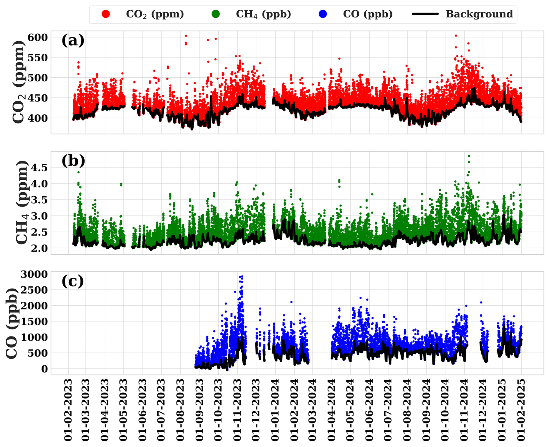
Figure 2 (a) Hourly averaged time series of atmospheric (a) CO₂, (b) CH₄, and (c) CO mole fraction for the study period (February 2023 to January 2025) over Sonipat. The thick black line represents the background mole fraction estimated using the ADVS method. CO₂ and CH₄ measurements were made using a Picarro GHG analyser, and CO measurements were made using CUPI-G sensor.

3.2 Seasonal variability

3.2.1 Seasonality of in situ observations

Figure 3 shows the monthly mean atmospheric CO₂ mole fractions during the study period. A shaded background has been used to distinguish the seasonal regimes used in this study. The monthly mean CO₂ mole fraction shows a maximum in November (post-monsoon season) and a minimum in August (monsoon season) in both years. The observed seasonal mean of CO₂ during different seasons were 440.8 ± 19.7 ppm (pre-monsoon), 422.6 ± 23.3 ppm (monsoon), 456.4 ± 30.8 ppm (post-monsoon), and 440.5 ± 19.7 ppm (winter).

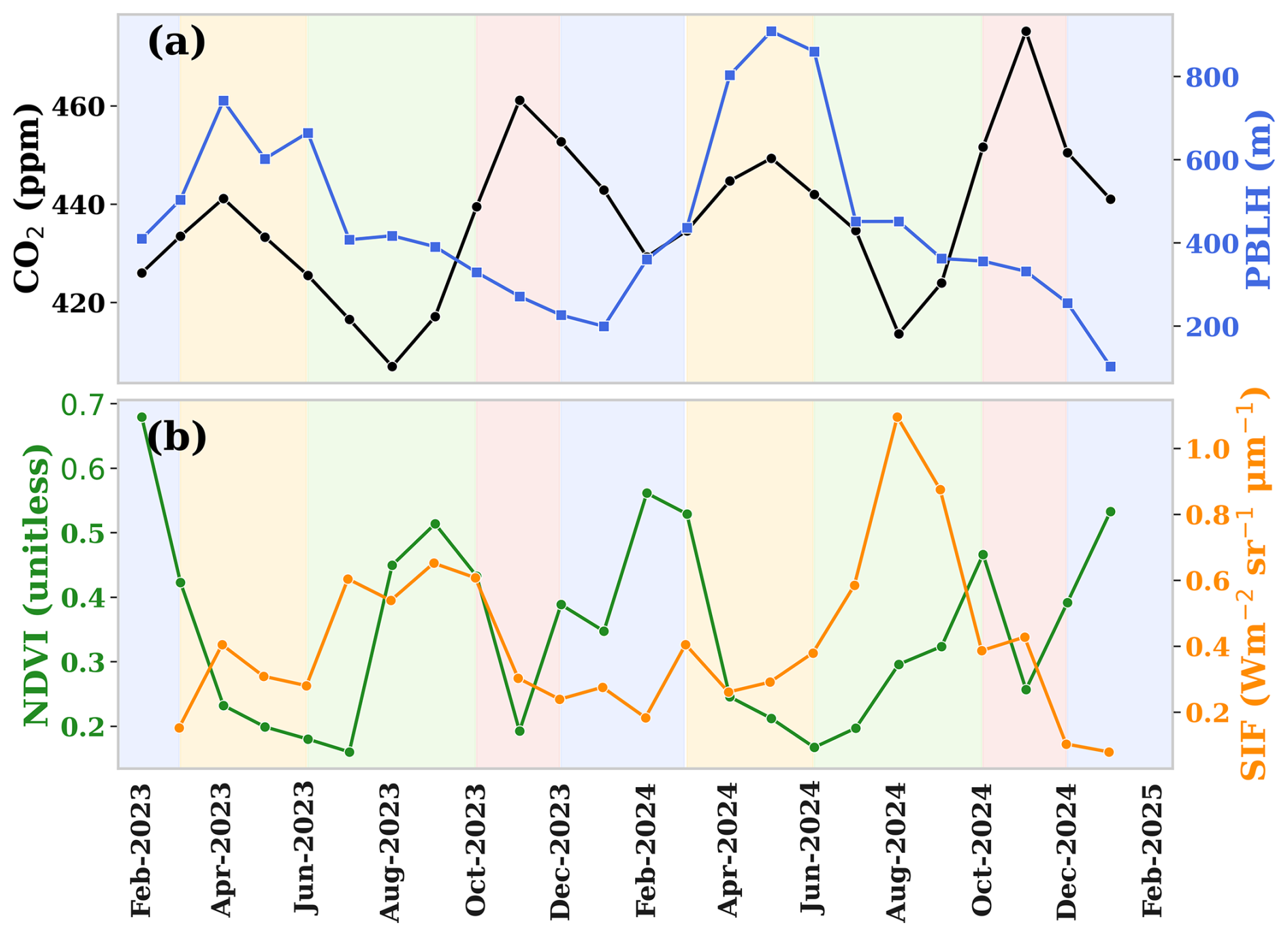
Figure 3 (a) Monthly variations of atmospheric CO₂ mole fraction (black) and PBLH (blue) and (b) NDVI (green) and SIF (orange) over the Sonipat monitoring station during the study period. The shaded background represents different seasons; yellow (pre-monsoon), green (monsoon), red (post-monsoon) and blue (winter).

The seasonal change in CO₂ mole fractions over the monitoring station is governed by the strength of emission sources, photosynthetic activity (biospheric fluxes), local meteorology and atmospheric transport. The planetary boundary layer height (PBLH), which is determined by local meteorology, strongly influences CO₂ mole fractions. PBL is the lowest layer within the troposphere, where temperature and wind speed variations are integral in modulating its height. During pre-monsoon, deep convection due to the well-developed PBLH from the surface to the upper troposphere results in lower mole fractions of CO₂, while the weakly developed PBLH in winter leads to higher CO₂ (Baker et al., 2012; Kar et al., 2004; Park et al., 2009; Patra et al., 2011; Randel and Park, 2006).

The seasonal change in CO₂ was examined using two different vegetation indices (normalised difference vegetation index, NDVI and solar-induced fluorescence, SIF) to assess the role of the biosphere in CO₂ mole fractions over Sonipat. Both NDVI and SIF have been widely used as indicators of vegetation cover and photosynthetic activity (Aburas et al., 2015; Nath, 2014). Our analysis shows a strong inverse relationship between CO₂ levels and NDVI, as illustrated in Fig. 3b. A noticeable decrease in atmospheric CO₂ mole fraction is observed at the onset of the monsoon (June), with increased vegetative activity continuing until September. Increased vegetation cover increases photosynthetic carbon uptake by the biosphere. However, as vegetation activity decreases from the post-monsoon to winter and pre-monsoon seasons, photosynthetic carbon uptake decreases, leading to a rise in atmospheric CO₂. Spearman's rank correlation analysis showed a weak and statistically insignificant relationship between CO₂ and NDVI ($\mathit{\rho }=-\mathrm{0.09}$, p=0.74). In contrast, CO₂ exhibited a moderate negative correlation with SIF ($\mathit{\rho }=-\mathrm{0.42}$, p=0.07). The negative correlation with SIF is consistent with enhanced biospheric uptake during periods of increased photosynthetic activity. Similar studies (Metya et al., 2021; Sreenivas et al., 2016; Tiwari et al., 2014), over India exhibited a strong dependence of CO₂ seasonality on local vegetative carbon uptake.

A sharp decrease in the seasonal mean (∼18 ppm) was noted from pre-monsoon to monsoon, attributed to enhanced photosynthetic activity around the measurement site, driven by abundant soil moisture. A further decrease in CO₂ mole fraction is also observed as the monsoon progresses, with minimum CO₂ mole fractions observed in August. The decreases in temperature (due to cloudy, overcast conditions prevailing during these months) reduce leaf and soil respiration, thereby enhancing carbon uptake (Jing et al., 2010; Patil et al., 2014). Further, an increase in CO₂ mole fraction (∼34 ppm) is observed during post-monsoon, reflecting higher ecosystem respiration (Sharma et al., 2014) and enhanced soil microbial activity (Fan and Forkel, 2025; Munksgaard et al., 2022), particularly from nocturnal respiration prior to crop harvest. The gradual decline in NDVI during this period indicates reduced CO₂ uptake by vegetation. This season coincided with crop-burning episodes in northern India, which significantly increased CO₂ mole fractions. A sharp decrease (∼16 ppm) in the seasonal mean during winter is evident compared to the post-monsoon. The shallow PBLH and winds from western IGP that transport crop-burning residue contribute to the enhanced mole fraction during winter. Table S2 in the Supplement compares the seasonal amplitude and the peak and drawdown months at the measurement site with those in similar studies across India. Sonipat exhibits higher seasonal amplitudes than other sites. However, a similar pattern in CO₂ peak and drawdown months is evident in other monitoring stations.

3.2.2 Seasonal constraints from model and satellites

Figure 4a shows the comparison of ground-based mole fraction of CO₂ with CarbonTracker inverse model (CT2022) simulated mole fraction (see different y axis). The model outputs beyond October 2023 were not publicly available. In general, the CT2022 model-simulated mole fractions are much lower than the observed mole fractions at the Sonipat station. The discrepancy is mainly due to the model's coarser resolution. Nevertheless, the model-simulated seasonal pattern of CO₂ mole fraction is broadly in agreement with observations (Fig. 4). The CT2022 model simulates a minimum mole fraction of 416 ppm in September, whereas in situ measurements show a minimum of 407 ppm in August. The CT2022 model exhibits higher mole fractions during the pre-monsoon season, consistent with in situ data. Note that most global and regional chemical transport models were unable to reproduce the large seasonal amplitude of surface-based measured atmospheric CO₂ mole fractions at any of the monitoring stations in India with different ecosystems (Lin et al., 2018; Philip et al., 2022).

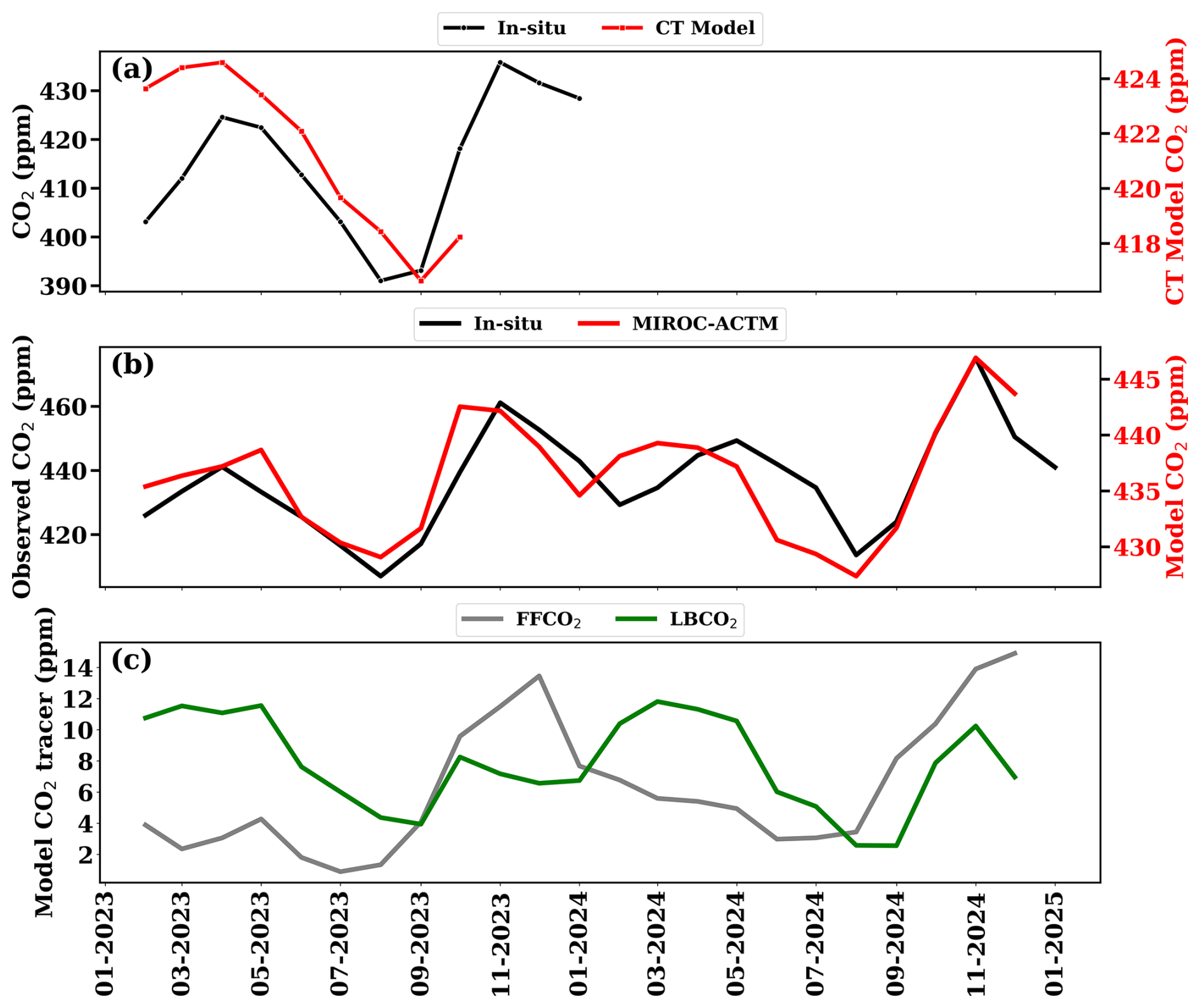
Figure 4 (a) Monthly mean background CO₂ mole fraction over Sonipat (estimated using the ADVS method) compared to CarbonTracker (CT2022) model-simulated values at daytime (13:00–16:00 IST). Note that the left y axis represents surface mole fraction from in situ measurements, and the right y axis represents CT2022-simulated mole fraction. (b) Comparison of simulated mole fraction of atmospheric CO₂ from MIROC-ACTM with in situ measurements at Sonipat and (c) monthly averaged time series of different tracers from the MIROC-ACTM.

Figure 4b shows the comparison of atmospheric CO₂ mole fractions over Sonipat with the simulated mole fraction of CO₂ from the MIROC4-ACTM model. Similar to CT2022, MIROC captures the seasonal pattern of CO₂, but fails to capture the actual seasonal amplitude over Sonipat. Figure 4c presents the monthly averaged time series of model-simulated CO₂ tracers. The fossil fuel tracer (FFCO₂) exhibits a peak in the post-monsoon period, followed by a gradual decrease through the end of winter. The shallow PBLH during this time traps vehicular emissions from NH-44 and industrial sources upwind of the monitoring station, resulting in higher FFCO₂. With the development of the PBLH in the pre-monsoon, FFCO₂ shows a gradual decrease, and rainfall during the monsoon results in minimum values during this time. The biospheric tracer (LBCO₂) shows a peak during the pre-monsoon, driven by dry soil conditions and a lack of vegetation and a drawdown during the monsoon. A sharp increase in LBCO₂ is observed during the post-monsoon season, coinciding with the harvest period at the monitoring station. Being surrounded by agricultural land, Sonipat is prone to emissions from crop residue burning around and upwind of the monitoring station. Both models underestimate these enhancements from regional sources.

Figure 5 compares XCO₂ from OCO-2 and OCO-3 satellites with ground-based CO₂ measurements at Sonipat during the study period. XCO₂ reveals a similar seasonal pattern with high mole fraction during the pre-monsoon season, followed by a drawdown in CO₂ mole fraction during the monsoon season and a further gradual increase in CO₂ during the post-monsoon and winter. Although the satellite column data captures the monthly variability reasonably well, it fails to capture the sharp increase in mole fraction during the post-monsoon. This post-monsoon enhancement from crop residue burning at the monitoring station, along with additional transport from Punjab, highlights the limitations of high-resolution satellite data in capturing local enhancements.

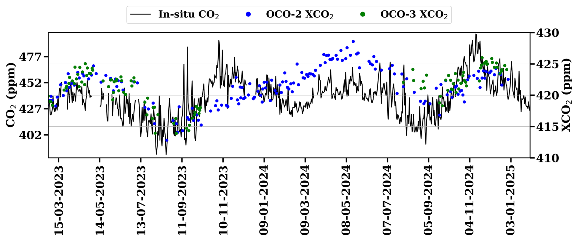
Figure 5 Daily variations of atmospheric CO₂ mole fraction from in situ measurements over Sonipat (left y axis) with column average CO₂ mole fraction (XCO₂) from the OCO-2 (ppm) and OCO-3 (ppm) satellite instruments (right y axis).

3.3 Diurnal variability

Figure 6a–d presents the averaged diurnal variation of atmospheric CO₂ mole fractions along with PBLH from ERA5 and Ceilometer at Sonipat during four seasons for the first year of the study (February 2023–January 2024). Figure S5 in the Supplement presents the diurnal variation for the second year of the study. The diurnal cycle has been analysed separately for each year, combining available PBLH data. All seasons exhibit a similar diurnal pattern, with maximum CO₂ mole fractions in the early morning hours (05:00–08:00 IST) and minimum mole fractions in the late afternoon hours (14:00–15:00 IST). The observed diurnal cycle of CO₂ is closely associated with the development of PBLH during the day (Fig. 6). The peak in CO₂ mole fraction during the morning hours can be attributed to the fumigation effect, and a well-mixed PBL dilutes CO₂ mole fractions during the afternoon hours.

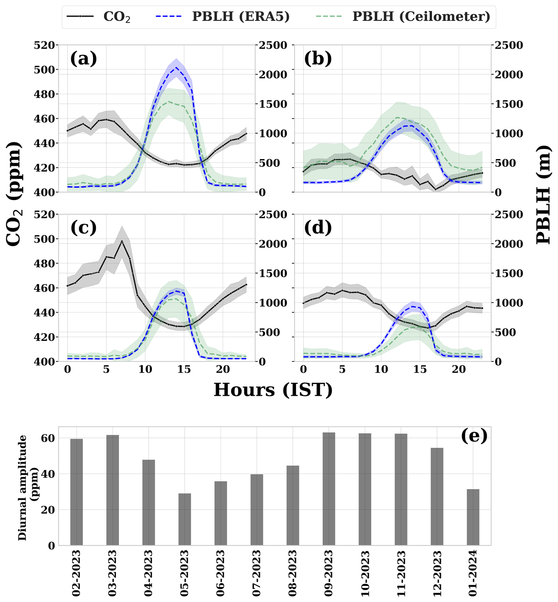
Figure 6 (a–d) Seasonally-averaged diurnal variation of atmospheric CO₂ over the Sonipat station during the pre-monsoon (MAM), monsoon (JJAS), post-monsoon (ON) and winter (DJF) seasons with planetary boundary layer heights (blue denotes PBLH from ERA5 and green denotes PBLH derived from Ceilometer), (e) monthly variation of the diurnal amplitude of CO₂ from February 2023 to January 2024.

Photosynthetic activity is another key driver of diurnal variability at Sonipat, a characteristic observed in rural areas with vegetative cover (Imasu and Tanabe, 2018). Strong vegetative uptake of CO₂ during the monsoon results in minimum daytime CO₂ mole fractions, and the lack of vegetation during post-monsoon contributes to maximum daytime CO₂ mole fractions during this season. The diurnal variation of GHGs reported by several studies (Nishanth et al., 2014; Patil et al., 2014; Sharma et al., 2014) from different parts of the country shows a similar trend. The same was observed for 2024 as well (Fig. S5). The diurnal variability of CO₂ over Sonipat is driven by biospheric activity and local meteorology.

Figure 6e shows the monthly average variation in diurnal amplitude (difference between the maximum and minimum mole fraction of CO₂ in the diurnal cycle) during the first year. The lowest diurnal amplitude of about 29 ppm is observed in May, while the highest amplitude at about 63 ppm is observed in September/October. We found that the post-monsoon season exhibited the highest diurnal variability (∼60 ppm), followed by the pre-monsoon (∼35 ppm), winter (∼30 ppm), and monsoon (∼20 ppm) seasons.

3.4 Drivers of CO₂ seasonality

The contribution of biospheric fluxes in driving the CO₂ mole fraction over Sonipat (for 2023) was analysed in Fig. 7. Figure 7a shows the simulated data from the Mi CASA biosphere model along with the monthly averaged mole fractions of CO₂ and daytime CO₂ (06:00–18:00 IST). Figure 7b presents the simulated NEE from GEOS-Chem and GPP from FluxSat, along with the monthly averaged mole fractions of daily-mean and nighttime CO₂ (18:00–06:00 IST). Positive NEE values indicate a net exchange of CO₂ from the biosphere to the atmosphere. On the other hand, a negative NEE value (when NPP exceeds Rh) suggests the uptake of CO₂ from the atmosphere to the biosphere.

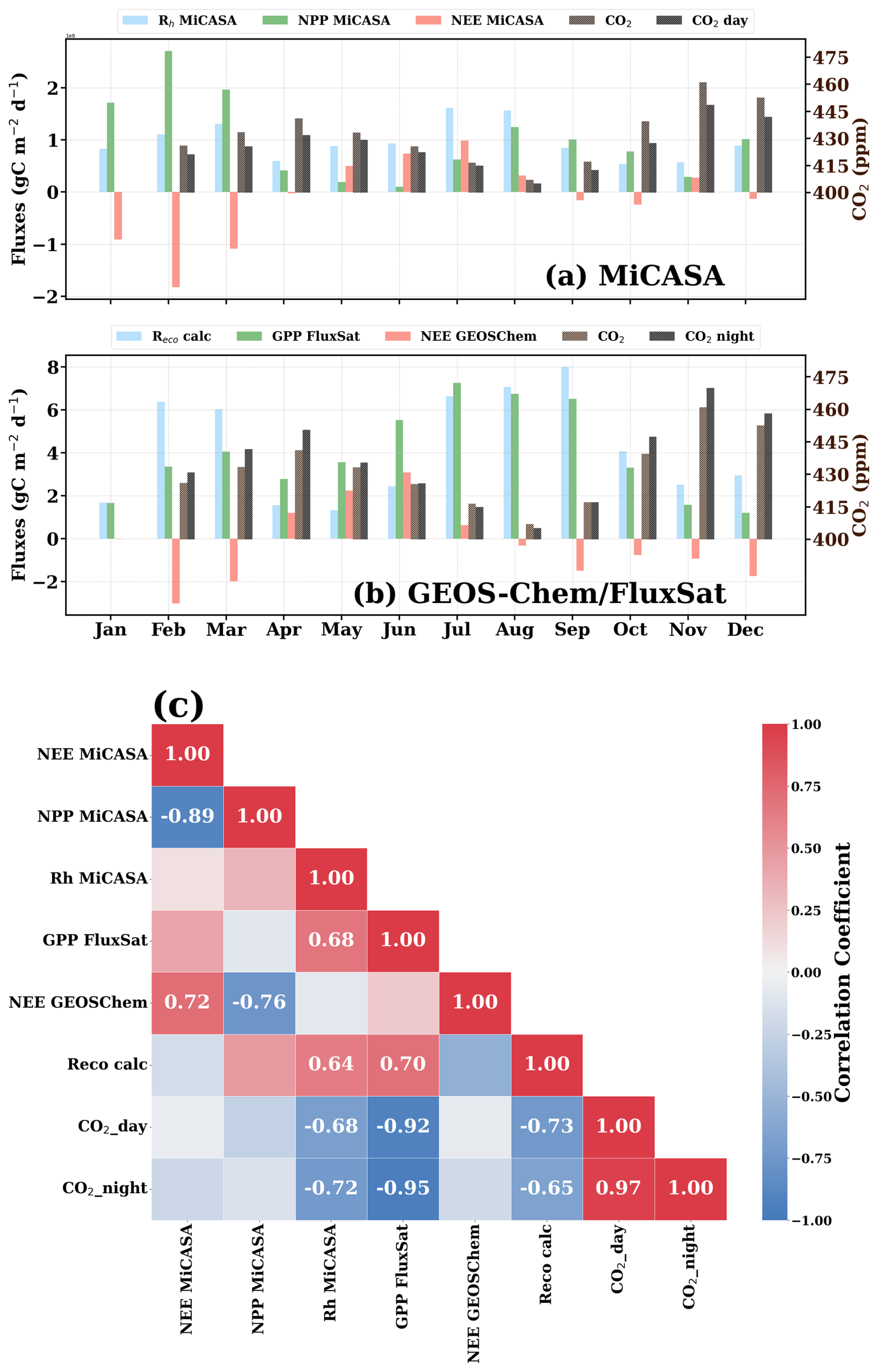
Figure 7 Monthly variation of atmospheric CO₂ mole fraction (for 2023) over the Sonipat monitoring station compared against (a) biospheric fluxes from the MiCASA terrestrial biospheric model and (b) GEOS-Chem model and FluxSat GPP data. (a, b) The CO₂ mole fraction are daytime mean (06:00–18:00 IST) and nighttime mean (18:00–06:00 IST). The correlation heatmap of all the variables. The annual growth rate of CO₂ has been subtracted from the CO₂ mole fraction using background data from the Mauna Loa observatory. The variable “Reco calc” was calculated as the difference between NEE (GEOS-Chem) and GPP (FluxSat). The Pearson correlation coefficients with a p value less than 0.05 have been displayed in the correlation plot.

The NEE flux shows a strong positive in June, followed by a gradual decrease through October (monsoon). During this time, Reco, Rh and GPP exhibit strong enhancements. These enhancements are accompanied by a drawdown of CO₂ during this time. The driving factor behind this CO₂ drawdown during monsoon is the enhanced ecosystem productivity during this time. Strong inverse correlations of GPP, Rh, and Reco with CO₂ suggested that the biosphere acts as a net sink of CO₂ (Fig. 8c).

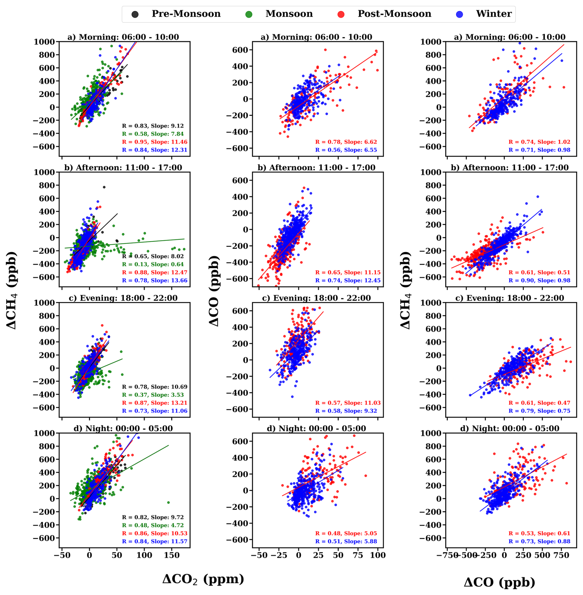
Figure 8 Tracer-tracer relations of $\mathrm{\Delta }{\mathrm{CO}}_{\mathrm{2}}/\mathrm{\Delta }{\mathrm{CH}}_{\mathrm{4}}$ (left panel), $\mathrm{\Delta }{\mathrm{CO}}_{\mathrm{2}}/\mathrm{\Delta }\mathrm{CO}$ (middle panel) and $\mathrm{\Delta }{\mathrm{CH}}_{\mathrm{4}}/\mathrm{\Delta }\mathrm{CO}$ (right panel) during (a) morning (06:00–10:00 IST), (b) afternoon (11:00–17:00 IST), (c) evening (18:00–22:00 IST) and (d) night (00:00–05:00 IST).

Interestingly, post-monsoon and winter months exhibit weak or negative NEE. This is because Rh values are low during these seasons due to drier soil conditions and lower soil moisture. It is also notable that GPP is very low during these months, which is associated with a high CO₂ mole fraction. Significant contributions of air-mass transport from upwind regions and boundary-layer dynamics, along with the lack of vegetation during this time, contribute to the buildup of CO₂ mole fraction.

3.5 Emission source detection using tracer-tracer relationships

The ratios (tracer-tracer) of GHGs have been widely used in previous studies to estimate different emission source contributions to atmospheric GHGs (Chandra et al., 2016, 2019; Lin et al., 2015; Lopez, 2012; Paris et al., 2008; Sreenivas et al., 2016, 2022). We followed a similar tracer-tracer correlation analysis to assess synoptic variation in CO₂ across different diurnal time windows and understand the emission sources contributing to CO₂ mole fractions over Sonipat (Fig. 8). The measurements have been divided into four-time windows: (a) morning hours (06:00–10:00 IST; the PBLH starts to develop after sunrise; local traffic is high), (b) afternoon hours (11:00–17:00 IST; the PBLH is well-developed; relatively minimum local traffic), (c) evening hours (18:00–22:00 IST; rush hour traffic and high household emissions), and (d) night hours (00:00–00:05 IST; relatively less anthropogenic emission sources). Excess mole fractions were used in the correlation analysis to remove the influence of background mole fractions on the correlation ratios (Worthy et al., 2009). The correlation between the different gases (CO₂, CH₄, and CO) has been studied using the robust linear fit regression method.

Figure 8 (left panel) presents the correlation of excess mole fraction of CH₄ and CO₂ during the four seasons. The ${\mathrm{CH}}_{\mathrm{4}}/{\mathrm{CO}}_{\mathrm{2}}$ correlation reveals a strong correlation (r>0.6) for all seasons except monsoon during all time windows, which suggests a similar source mechanism or a controlling emission process for both gases at the measurement site. Around the monitoring station, vehicular emissions from the nearby highway and natural gas combustion emissions are possible sources. Also, a positive correlation suggests that anthropogenic emissions dominate the carbon cycle in Sonipat (Fang et al., 2015). The regression slope shows strong diurnal variation throughout all seasons. Recent studies across India have reported similar results, with higher regression slopes during the post-monsoon and winter seasons than during the pre-monsoon and monsoon seasons (Lin et al., 2015; Sreenivas et al., 2016, 2022).

Figure 8 (middle panel) presents the correlation of excess mole fractions of CO and CO₂ during post-monsoon and winter. The $\mathrm{CO}/{\mathrm{CO}}_{\mathrm{2}}$ ratio over Sonipat (4–12.5 ppb ppm⁻¹) is lower than that for fresh plumes from wildfire (Andreae and Merlet, 2001; Mauzerall et al., 1998) and much lower than that from biomass burning events alone (Matsueda et al., 1999). Lin et al. (2015) reported $\mathrm{CO}/{\mathrm{CO}}_{\mathrm{2}}$ ratios of 13 ppb ppm⁻¹ over Southeast Asian outflow from February to April 2001. This value was found to be influenced by fossil fuel emissions (Russo et al., 2003), crop residue burning, and biofuel burning rather than solely by biomass/biofuel burning. The $\mathrm{CO}/{\mathrm{CO}}_{\mathrm{2}}$ ratios over Sonipat during the post-monsoon and winter closely match those of Lin et al. (2015), suggesting that the high CO₂ mole fractions during this time are an interplay of different sources like crop residue burning (long-range transport) and other fossil-fuel emissions (vehicular and industrial) around the monitoring station.

Figure 8 (right panel) presents the correlation of excess mole fractions of CH₄ and CO during post-monsoon and winter. The ${\mathrm{CH}}_{\mathrm{4}}/\mathrm{CO}$ ratios range from 0.3 to 1.2 at Sonipat, indicative of anthropogenic emission sources (Bakwin et al., 1995; Harriss et al., 1994; Lai et al., 2010; Lin et al., 2015; Niwa et al., 2012; Sawa et al., 2004; Wada et al., 2011; Xiao et al., 2004). In contrast, ratios influenced solely by biomass and biofuel burning are much lower, ranging from 0.07 to 0.3 (Andreae and Merlet, 2001; Mauzerall et al., 1998; Mühle et al., 2002).

These lower ratios highlight the significant difference when compared to the values recorded in Sonipat. Moreover, very high CH₄ emissions from livestock can elevate the generally low ${\mathrm{CH}}_{\mathrm{4}}/\mathrm{CO}$ ratios associated with biomass burning. This indicates substantial contributions from various CH₄ sources apart from biofuel burning.

4 Discussions

By investigating two years of high-frequency atmospheric CO₂ mole fraction measurements at the Sonipat station in the IGP region, we identified the following salient features about the seasonality, diurnal variability, drivers of temporal variability, and emission sources of CO₂.

Very high atmospheric CO₂ mole fractions over IGP. The surface-based measurements of atmospheric CO₂ mole fraction exhibit strong seasonality, with a maximum (456.4 ppm) during post-monsoon and a minimum (407.2 ppm) during monsoon, with an average of 422.6 ppm. Seasonal changes in the PBLH affected the atmospheric CO₂ mole fraction by diluting or concentrating GHG mole fractions near the surface. A strong dependence of CO₂ seasonality on local vegetative carbon uptake was observed from the negative correlation between NDVI and CO₂ mole fractions, which was consistent across India (Metya et al., 2021; Sreenivas et al., 2016; Tiwari et al., 2014).

A comparison of the seasonality of atmospheric CO₂ at Sonipat with other Indian and global sites in the same latitudinal band revealed very high seasonality at Sonipat, surpassing that of all other stations. This high seasonality is attributed to elevated CO₂ mole fractions in November (post-monsoon), driven by local emissions and crop residue burning. Figure 9a presents the monthly averaged variation of CO₂ over Sonipat during the study period (SNT) with other measurement sites in the same latitudinal band (5–40° N). Details of all monitoring stations used in this study are described in detail in Sect. S2. Sonipat exhibits a very high seasonal amplitude (∼60 ppm) compared to other sites worldwide (∼15 ppm, see Fig. 9b), attributed to the sharp increase in post-monsoon, consistent in both years of the study (see Fig. 2). Excluding November would reduce the seasonal amplitude of Sonipat to 35 ppm, which is comparable to that in Ahmedabad (35 ppm). Temperature-driven PBLH (which inhibits mixing) and strong north-westerly winds (which induce transport of emissions from upwind) during this season play a key role in these high CO₂ mole fractions (Figs. S3 and S4 in the Supplement). It is also noted that the CO₂ drawdown in August is primarily due to the green paddy fields during the monsoon (terrestrial CO₂ uptake), coinciding with heavy rains that wash out CO₂. This combined effect makes the lowest CO₂ mole fractions in Sonipat comparable to those at some background stations across the globe with different ecosystems (Fig. 9a).

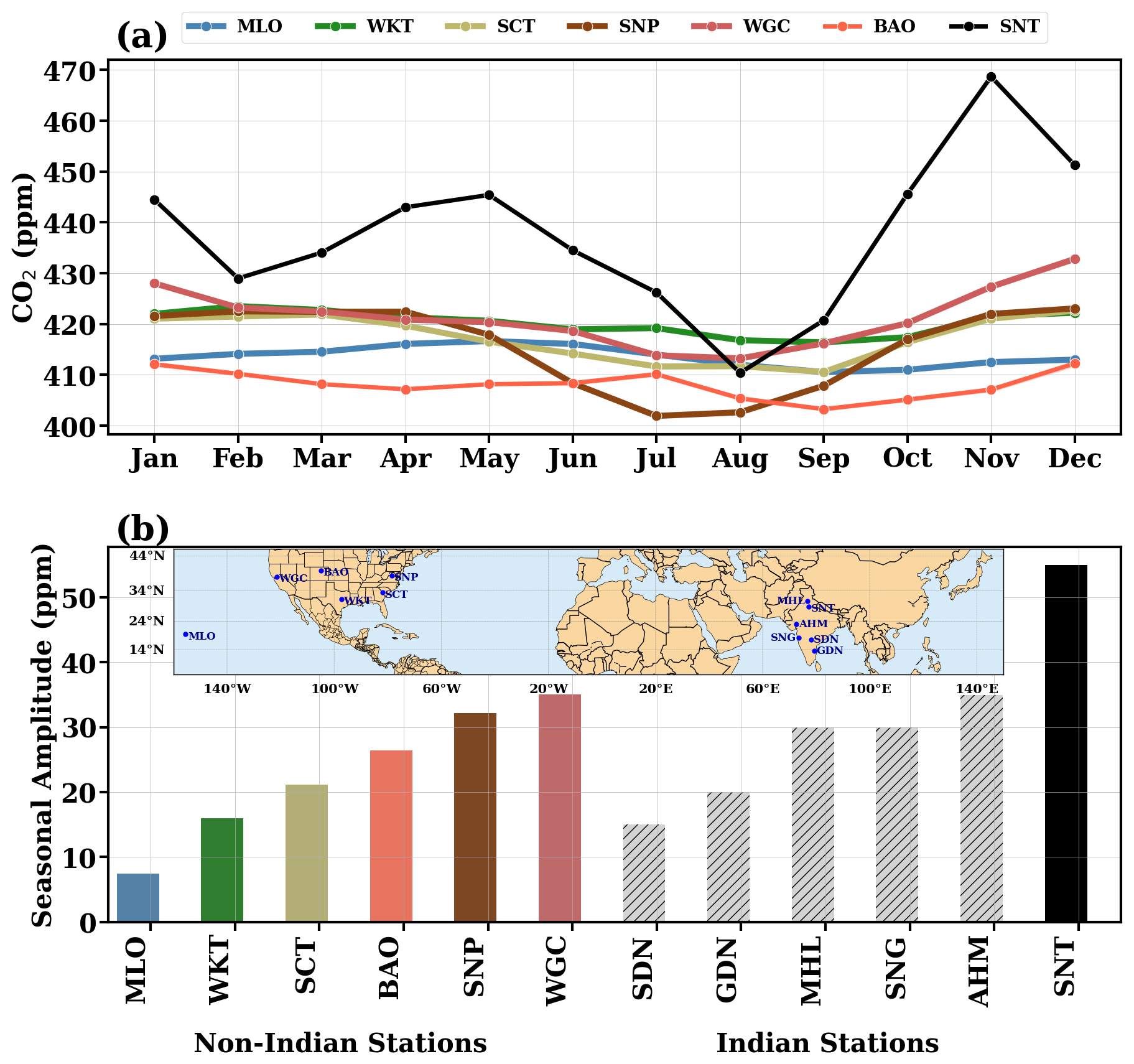
Figure 9 (a) Comparison of the seasonal variability of atmospheric CO₂ over Sonipat monitoring station with various locations in the same latitudinal band. (b) Comparison of the seasonal amplitude between Indian (coloured bars) and international monitoring stations (grey bars). Indian stations include Shadnagar (SDN), Sinhagad (SNG), Ahmedabad (AHM), Mohali (MHL), Gadanki (GDN), and Sonipat (SNT). International stations include Mauna Loa (MLO), South Carolina (SCT), Shenandoah National Park (SNP), Walnut Grove, (WGC), Moody (WKT) and Boulder (BAO). For all international stations except BAO, the five-year average (2018–2022) has been chosen for the seasonality. For BAO, 2011–2016 has been used due to lack of coinciding data. The monthly average of the entire study period (February 2023–January 2025) has been used for this comparison.

This study also analysed the drivers of this variability using various ecosystem variables, including NEE, which represents the net carbon exchange between terrestrial ecosystems (the difference between Rh and NPP). NPP is the net amount of CO₂ retained in the biosphere. Rh is the amount of CO₂ emitted into the atmosphere due to the decomposition of organic matter by microorganisms in the soil. Reco, the sum of Ra (autotrophic respiration) and Rh has been calculated as the difference of FluxSat GPP and GEOS-Chem NEE. GPP, a measure of carbon uptake by plants, was observed to be very high during monsoon along with NEE, Rh and Reco. Statistical analysis revealed a strong negative correlation of GPP with CO₂ and a strong positive correlation with Rh and Reco. These suggest that the primary sink of CO₂ over Sonipat is biospheric activity, driven by the abundance of vegetation resulting from enhanced soil moisture during the monsoon.

Performance of models and satellites over IGP. Although both the CarbonTracker and MIROC-ACTM models captured the broad seasonal pattern of CO₂ mole fractions, they substantially underestimated it. However, MIROC showed greater seasonal variability than CT2022, with post-monsoon highs and pre-monsoon drawdowns showing strong correlations with in situ measurements. Further analysis of the tracers from MIROC provides insights into the driving factors of this variability. The post-monsoon peak is attributed to vehicular emissions from the nearby highway and industrial sources upwind of the monitoring station. The drawdown in monsoon is attributed to the added soil moisture and increased CO₂ uptake by plants during this time. The location of the measurement site in IGP, downwind of Punjab, provides insights into this transport-induced enhancement. The OCO-2 and OCO-3 satellite XCO₂ retrievals also showed similar seasonal variability; however, the satellites could not capture CO₂ enhancements from local sources.

Diurnal variability driven by meteorology. The atmospheric CO₂ mole fraction at Sonipat exhibits a consistent diurnal pattern across seasons. It was observed that CO₂ mole fractions steadily increased throughout the night, reaching a peak in the early morning hours. This accumulation of CO₂ during the night-time can be attributed to the fumigation effect: a significant rise in surface mole fractions, notable during the early morning hours due to the breakdown of the nocturnal inversion layer following sunrise (Stull, 1988). Weak winds and shallow PBLH enhance the fumigation effect. The combined effect of photosynthetic activity and mixing of PBLH during the afternoon hours drives the CO₂ mole fractions during different seasons. The diurnal amplitude shows large month-to-month variation with an increasing trend from May to September 2023 and a decreasing trend till February 2024. Figure S6 in the Supplement presents the seasonal variation of CO₂ compared with PBLH derived from Ceilometer and ERA5 reanalysis data for 2023. A slight shift in the timing of the morning peaks was observed from season to season, due to changes in sunrise time, which affected photosynthetic activity.

Detecting emission source contributions. Tracer-tracer relationships across different time periods during the post-monsoon and winter seasons were examined. Analysis reveals that CO₂ and CH₄ exhibit a strong positive correlation across all seasons, suggesting common sources for both gases. During monsoon season, the afternoon time window shows a weak correlation with other time windows, revealing distinct source and sink mechanisms for CO₂ and CH₄, such as CH₄ loss via hydroxyl radical and CO₂ uptake by plants. The regression slope is higher during the post-monsoon and winter months, when reduced photosynthetic activity and the dominance of local emissions and long-range transport are observed. The lower values during pre-monsoon and monsoon are associated with the dominance of vegetation and terrestrial uptake of CO₂ by photosynthetic activity.

The $\mathrm{CO}/{\mathrm{CO}}_{\mathrm{2}}$ correlation shows strong diurnal variability, suggesting the dominance of different source mechanisms throughout the day, with strong correlation during the morning and afternoon hours (suggesting a similar source) and weaker correlation during the evening and night hours (suggesting different sources). The post-monsoon season shows higher regression slopes due to reduced photosynthetic activity. Over Sonipat, the contribution of CO and CO₂ from long-range airmass transport (influenced by crop residue burning in Punjab) during post-monsoon from the northwest of the monitoring station is diluted by other sources (such as vehicular emissions from highways, crop residue burning, and open burning). The contribution of biofuel burning (which has a higher burning efficiency) during post-monsoon and winter (Andreae and Merlet, 2001) can also reduce the $\mathrm{CO}/{\mathrm{CO}}_{\mathrm{2}}$ ratios. Figure S4 presents the wind patterns during the different seasons, revealing the predominant winds from the northwest during the post-monsoon season. The $\mathrm{CO}/{\mathrm{CO}}_{\mathrm{2}}$ ratios reveal the combined influence of various sources around and upwind of the monitoring station during the post-monsoon period.

The ${\mathrm{CH}}_{\mathrm{4}}/\mathrm{CO}$ correlation (r>0.7) was stronger during winter than during post-monsoon across all time windows, suggesting similar sources during winter and different sources during post-monsoon. The regression slope was higher during winter than during the post-monsoon period. This was traced to the lack of photosynthetic activity and the dominance of local emissions and long-range transport. Lin et al. (2015) reported comparable ${\mathrm{CH}}_{\mathrm{4}}/\mathrm{CO}$ ratios at Pondicherry (PON) and Port Blair (PBL). CH₄ and CO emissions from biomass, biofuel burning and livestock estimated from EDGAR v4.2, 2011 indicate a ${\mathrm{CH}}_{\mathrm{4}}/\mathrm{CO}$ ratio of 0.64–0.69 over the Indian subcontinent from 2000–2008. These ratios are comparable to those observed during both seasons at Sonipat.

In summary, this study demonstrated that this high temporal CO₂ variability across the IGP region arises from an interplay of local anthropogenic and biomass-burning emissions, biospheric fluxes, and prevailing meteorology.

5 Conclusions

In this study, we conducted high frequency measurements of atmospheric CO₂ mole fractions at a suburban station in the Indo-Gangetic Plain, Sonipat and investigated the carbon cycle dynamics over IGP. The atmospheric CO₂ mole fractions from February 2023 to January 2025 have been measured using a GHG analyser with laser-based cavity ring-down spectroscopy. CO₂ molefractions over Sonipat recorded an annual average of 440.8 ± 19.7 parts per million (ppm) in 2024, with a very high seasonal variability of ∼60 ppm, much higher than that of other monitoring stations in the same latitudinal band. Post-monsoon recorded the highest diurnal variability (∼60 ppm) and monsoon recorded the least (∼20 ppm) with a consistent diurnal pattern irrespective of season. By examining a series of observational and modelling data, such as ground-based and satellite-based measurements, three model outputs, ecosystem proxy variables, and the tracer-tracer analysis technique, we identified the drivers of the high temporal variability of CO₂ over Sonipat and the IGP region. First, this high seasonality is attributed to elevated CO₂ mole fractions in November (post-monsoon), driven by local emissions and crop residue burning. We found that biospheric activity was the primary driver of seasonal changes over Sonipat, with anthropogenic emissions and soil respiration as the major sources and photosynthetic carbon uptake as the major sink. In addition, boundary-layer dynamics and air-mass transport from upwind regions significantly contribute to the buildup of CO₂ mole fraction. Second, we found that although both the CarbonTracker and MIROC-ACTM models captured the broad seasonal pattern of CO₂ mole fractions, they substantially underestimated it. Moreover, the OCO-2 and OCO-3 satellite XCO₂ retrievals also showed similar seasonal variability; however, the satellites could not capture CO₂ enhancements from local sources. Third, we found that the atmospheric CO₂ mole fraction at Sonipat exhibits a consistent diurnal pattern irrespective of season, with a maximum during the morning hours, attributed to the fumigation effect, followed by a gradual decrease during the day and a minimum during the afternoon hours, when photosynthetic activity is enhanced. Finally, tracer-tracer relationships across different time periods in the post-monsoon and winter seasons revealed common sources of CO₂ and CH₄. The $\mathrm{CO}/{\mathrm{CO}}_{\mathrm{2}}$ ratios reveal the combined influence of vehicular emissions, crop residue burning, and open burning on CO₂ mole fractions in Sonipat during the post-monsoon period. This study identified key sources and drivers of the high CO₂ temporal variability in a data-sparse IGP region. These findings advance our understanding of carbon cycle dynamics, with direct implications for mitigation and policy.