Deciphering the impacts of meteorology on surface ozone variability in eastern China using explainable machine learning models

Understanding how meteorology influences surface ozone variability is critical for interpreting trends and designing effective air quality policies. This study employs explainable machine learning (XML) with SHapley Additive exPlanations (SHAP) to interpret daily ozone variations from 2013 to 2023 across three major regions in eastern China: North China Plain (NCP), Yangtze River Delta (YRD), and Pearl River Delta (PRD). An ensemble of five machine learning models (LightGBM, XGBoost, CatBoost, Random Forest, and Extra Trees) is trained using 14 meteorological variables and two temporal indicators. XML reveals nonlinear, region-specific ozone-meteorology relationships that are broadly consistent with physical understanding, while differences in SHAP attributions across algorithms highlight structural uncertainty arising from multicollinearity among input variables. We use SHAP-derived contributions to attribute warm-season ozone trends to meteorological versus non-meteorological drivers. Before 2019, ozone increases are mainly associated with the temporal proxy for non-meteorological influences (e.g., emission changes), whereas after 2019 meteorological variability dominates regional ozone trends. Exploiting the additive nature of SHAP, we develop a de-weathering framework that partitions daily ozone into a SHAP-based climatological baseline and a meteorology-induced ozone anomaly (MOA). Across all three regions, the magnitude of positive MOA events increases over 2013–2023, while their frequency and duration show no significant trends, indicating that meteorological conditions increasingly amplify the intensity of ozone pollution episodes, without a corresponding increase in their frequency or duration. Our results demonstrate both the utility and limitations of XML for disentangling meteorological drivers of ozone pollution and provide new constraints on how meteorology shapes surface ozone under China's clean air actions.

1 Introduction

Surface ozone is a major air pollutant that threatens human health and ecosystems (Cohen et al., 2017; Fowler et al., 2009; Mills et al., 2018; Zhang et al., 2019). It is formed mainly through photochemical reactions involving precursors such as carbon monoxide (CO), nitrogen oxides (NO_x = NO + NO₂), and non-methane volatile organic compounds (NMVOCs) under sunlight. In China, nationwide monitoring has revealed a widespread and rapid increase in surface ozone levels since 2013, drawing growing attention from researchers and policymakers (Lu et al., 2020; Wang et al., 2017). The Chinese government has implemented a series of clean air actions since 2013 to reduce anthropogenic emissions of air pollutants (State Council of the People's Republic of China, 2013, 2018). Early emission control efforts (2013–2017) primarily targeted PM_2.5 and NO_x reductions, which may have contributed to ozone increases under the VOC-limited photochemical conditions prevalent in eastern Chinese cities. In the subsequent phase (2018–2020), integrated VOC and NO_x controls were implemented to address ozone pollution (Liu et al., 2023; Wang et al., 2023).

Ozone formation is highly sensitive not only to chemical precursors but also to meteorological conditions. Temperature and solar radiation control photochemical production rates, while wind speed, boundary-layer height, and large-scale circulation determine the dispersion, accumulation, and transport of ozone and its precursors (Fiore et al., 2012; Lu et al., 2019). Relative humidity, cloud cover, and precipitation further modulate ozone lifetimes and vertical mixing (Fu and Tian, 2019; Lu et al., 2019). Recent studies have shown that meteorological variability can explain a substantial fraction of interannual ozone changes in China and can even mask or amplify the effects of emission controls in some years (Liu and Wang, 2020; Liu et al., 2023; Weng et al., 2022). Thus, explicitly isolating and quantifying the meteorological contribution to surface ozone variability is critical for correctly interpreting observed ozone trends and evaluating the effectiveness of clean air policies.

Conventional approaches for quantifying meteorological impacts on surface ozone include statistical models, such as multiple linear regression, generalized additive models (Bloomer et al., 2009; Gong et al., 2017), and numerical atmospheric models that perturb selected variables to attribute ozone changes to specific processes (e.g., Liu et al., 2023; Liu and Wang, 2020). These approaches suggest that worsening meteorological conditions – particularly higher temperatures and lower humidity – have contributed significantly to the rising surface ozone levels in eastern China since 2012, with impacts comparable to those of anthropogenic emissions (Liu et al., 2023; Liu and Wang, 2020). Temperature plays a particularly important role in northern China by directly enhancing ozone formation and increasing anthropogenic and biogenic precursor emissions (Dang et al., 2021; Wu et al., 2024), whereas humidity is found to be especially influential in central and southern China (Han et al., 2020; Li et al., 2020). However, both statistical and numerical models face key limitations in quantifying meteorological contributions. Linear statistical models can approximate the dominant relationships and meteorology-driven trends in ozone at seasonal or annual scales (e.g., Weng et al., 2022), yet they have limited flexibility to represent complex nonlinear interactions. Process-based models, on the other hand, are computationally intensive and often exhibit biases relative to observed ozone concentrations (Travis and Jacob, 2019; Ye et al., 2022). Moreover, they rely heavily on emission inventories, which are typically updated on multi-year timescales, limiting their ability to reflect recent changes in emissions and to provide a comprehensive understanding of their impacts on ozone chemistry.

Machine learning (ML) and emerging explainable ML (XML) techniques provide a powerful framework for capturing the complex, nonlinear relationships between observed meteorological variables and surface ozone concentrations, thereby addressing some of the limitations of traditional statistical and process-based methods. XML information can be broadly categorized into global and local explainability (Flora et al., 2024). Global explainability characterizes how input features influence model predictions across the dataset, often by ranking input features in terms of importance, for example using feature-importance outputs from Random Forest, which have been widely applied to identify key meteorological drivers of surface ozone in China (Ma et al., 2021; Weng et al., 2022; Zhan et al., 2018). In contrast, local explainability attributes individual predictions to specific input features, offering more detailed insights into input–output dependencies at the data-point level. Recently, the SHapley Additive exPlanation (SHAP) technique has been applied to ML models to separate meteorological, chemical, and source-related effects on ozone in individual regions, such as Hangzhou (Yao et al., 2024; Zhang et al., 2024), Shenzhen (Mai et al., 2024), and Taipei (Li et al., 2025). These works demonstrate the potential of XML for ozone attribution at the city or regional scale.

Despite recent progress, the application of XML techniques to systematically understand meteorological influences on ozone remains limited. Key challenges include assessing XML's ability to capture ozone–meteorology relationships across spatiotemporal scales and evaluating the consistency of explanations across different ML algorithms. In this study, we address these challenges by combining an ensemble of five SHAP-interpreted ML models with a new de-weathering framework to analyze daily surface ozone across three regions in eastern China from 2013 to 2023. Specifically, we (1) quantify nonlinear ozone–meteorology relationships and evaluate the robustness of XML explanations across five tree-based models; (2) use SHAP values to attribute long-term warm-season ozone trends to meteorological versus non-meteorological factors; and (3) develop a SHAP-based de-weathering approach that partitions daily ozone into a climatological baseline and meteorology-induced ozone anomalies (MOA), allowing trends in the intensity and occurrence of meteorology-driven ozone events to be diagnosed. These advances enable a more comprehensive assessment of how meteorology shapes ozone variability under China's clean air actions.

2 Data and Methods

2.1 Surface ozone measurements and meteorology reanalysis

We use nearly 11 years of surface ozone measurements (from 1 January 2013 to 30 September 2023, 3925 d in total) collected by the national air-quality monitoring network operated by the Chinese Ministry of Ecology and Environment (https://air.cnemc.cn:18007, last access: 4 October 2024). The ozone exposure metric is the daily maximum 8 h average (MDA8), calculated for each site on each day. Data quality control procedures are applied to remove outliers, following Lu et al. (2018). Specifically, we discard extremely high hourly ozone concentrations, require a sufficient number of valid hourly measurements to compute daily MDA8, and exclude sites with substantial data gaps over the study period (Lu et al., 2018). The measurement sites are then averaged by each city to account for air quality condition at the city level. The number of monitoring sites per city varies from 3 to 27. Here, we focus our analyses on three populous regions in eastern China: the North China Plain (NCP), the Yangtze River Delta (YRD), and the Pearl River Delta (PRD). The locations of the cities and the regional mean MDA8 ozone concentrations are shown in Fig. 1.

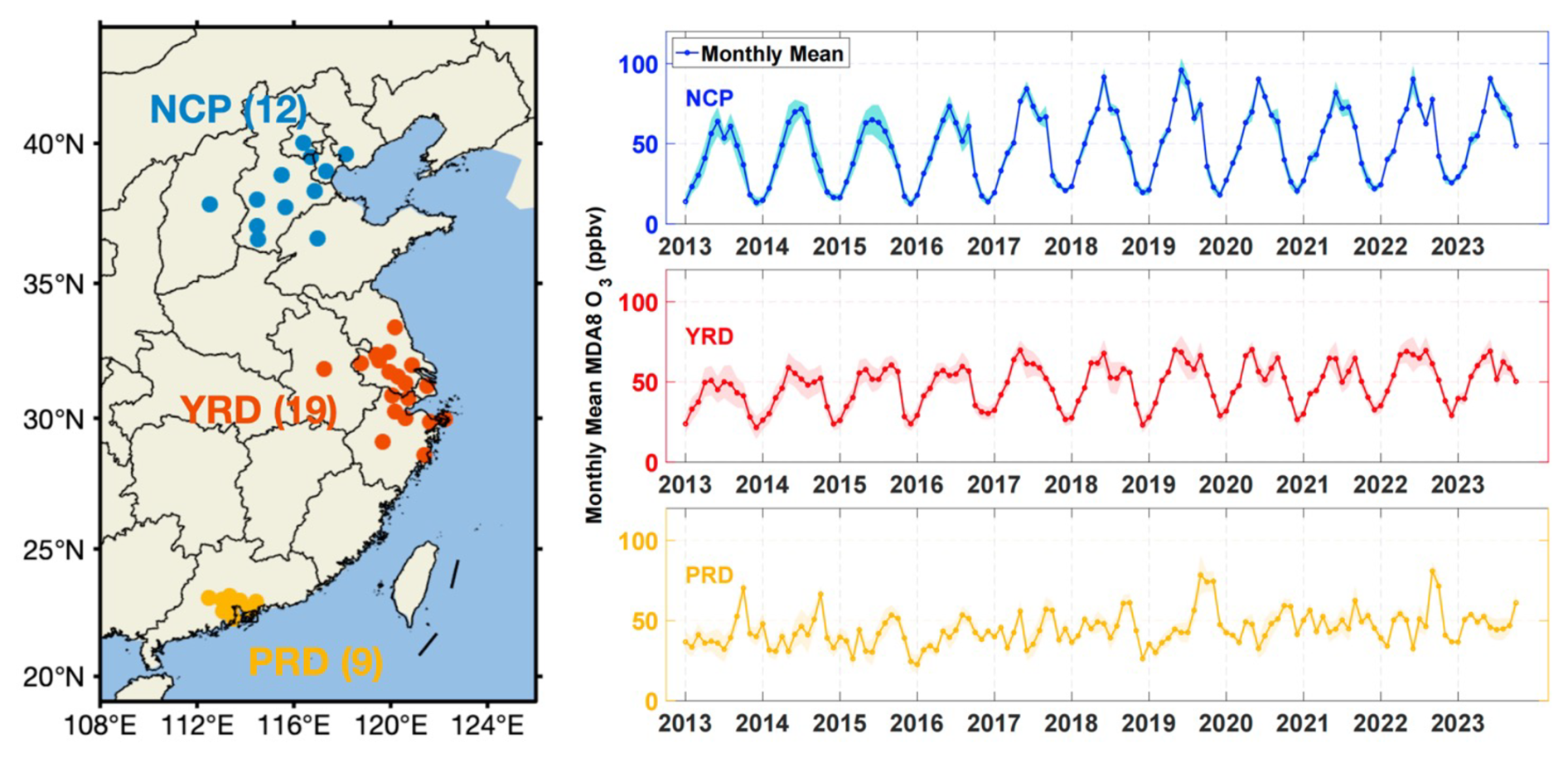
Figure 1 Locations of ozone monitoring cities and regional averaged monthly MDA8 ozone concentrations analyzed in this study. The three regions are North China Plain (NCP, blue), Yangtze River Delta (YRD, Red), and Pearl River Delta (PRD, yellow). Numbers in brackets denote the number of cities. The right panels show monthly mean ozone concentrations in the three regions over January 2013 to September 2023. Shaded areas represent ±1 standard deviation across cities within each region.

In this study, we use 14 meteorological variables as input features: 2 m temperature (T2M), surface incoming shortwave solar radiation (SWGDN), northward wind at 850 hPa (V850), eastward wind at 850 hPa (U850), 10 m wind speed (W10M), geopotential heights at 500 hPa (H500) and 850 hPa (H850), surface pressure (PS), surface evaporation (EVAP), surface relative humidity (RH), total surface precipitation flux (PRECTOT), planetary boundary-layer height (PBLH), total cloud fraction (CLDTOT), and surface albedo (ALBEDO). These variables are selected based on their strong correlations with daily surface ozone variations, as established in previous modelling and statistical studies (Liu and Wang, 2020; Liu et al., 2020; Mo et al., 2020; Requia et al., 2020).

The meteorological data are obtained from the Modern-Era Retrospective Analysis for Research and Applications, version 2 (MERRA-2) reanalysis (Gelaro et al., 2017), which provides hourly global fields at 0.5° × 0.625° resolution. To match each ozone monitoring site, we use its latitude–longitude coordinates to identify the nearest MERRA-2 grid cell and extract the corresponding 24 h mean meteorological variables from that grid cell for each day. When multiple sites fall within the same MERRA-2 grid cell, they share the same meteorological inputs at the grid scale. Meteorological variables are also averaged at the city level to ensure consistency with the ozone observations used for model training. Using city-level ozone and meteorological conditions helps reduce representativeness errors between point measurements and coarse-resolution reanalysis data. In addition, sensitivity tests show that using only one site per city does not materially affect model performance or the subsequent analyses.

2.2 ML models and explainability

We apply five ML algorithms: LightGBM (Ke et al., 2017), XGBoost (Chen and Guestrin, 2016), CatBoost (Prokhorenkova et al., 2018), Random Forest (Breiman, 2001), and Extremely Randomized Trees (Extra Trees; Geurts et al., 2006), to predict daily variations in surface ozone. All five are tree-based ensemble models that utilize decision trees as their basic structure. LightGBM, XGBoost, and CatBoost are gradient-boosting methods, which iteratively train trees to correct errors from previous iterations. In contrast, Random Forest and Extra Trees employ bagging, where multiple trees are trained independently on random subsets of the data and input features, and their predictions are then averaged to produce the final output. We select these tree-based models because their structure is highly compatible with SHAP-based explainability methods, which can efficiently compute feature contributions by exploiting decision-tree ensembles.

The output variable for all models is the daily MDA8 ozone concentration. To construct the ML models, in addition to the 14 meteorological variables introduced in Sect. 2.1, two temporal features are included: the day of year (DOY), which ranges from 1 to 365 (or 366 in leap years) and captures the seasonal ozone cycle, and a UNIX time variable, defined as a continuous, non-repeating count of days since 1 January 2013. The UNIX term serves as a proxy for slowly varying, non-meteorological influences such as long-term changes in anthropogenic emissions and background concentrations (Vu et al., 2019). While 14 meteorological predictors may appear numerous, the large sample sizes (∼35 000–74 000 samples per region) provide sufficient statistical power to support model training without overfitting. In addition, tree-based ensemble methods inherently mitigate multicollinearity through bootstrap aggregation and random feature subsampling (Breiman, 2001, Chen and Guestrin, 2016). We examine the correlations among all input variables (14 meteorological predictors, DOY, and UNIX) using a Pearson correlation matrix (Fig. S1 in the Supplement). As expected, several variables are moderately to strongly correlated (for example, between surface temperature and solar radiation, or among wind-related variables), reflecting the coupled nature of boundary-layer dynamics, radiation, and circulation. We retain these correlated variables in the models because they represent physically distinct but linked processes that can each modulate ozone formation and transport.

We train separate ML models for each region using all available monitoring sites to ensure sufficient data coverage. The datasets are split randomly into 90 % for training and 10 % for testing. Hyperparameters are optimized using five-fold cross-validation based on the coefficient of determination (R²). For explainability analysis, we use the training data rather than the test data, as the goal is to understand how the model relies on input features rather than its generalization performance (Flora et al., 2024; Lakshmanan et al., 2015). Therefore, after model evaluation, we retrain each model on the full dataset before applying XML techniques. Hyperparameters for ML models are listed in Table S1 in the Supplement.

We use the SHAP method (Lundberg and Lee, 2017) to quantify the contribution of each input feature to ozone variability. SHAP is grounded in cooperative game theory and provides local explainability by assigning each feature a contribution value for individual predictions. For a given ML model, the predicted MDA8 ozone concentration on the dth day in year y in a specific region (${{\mathrm{O}}_{\mathrm{3}}\mathrm{ori}}_{y,d}$) can be expressed as,

$$\begin{array}{}\text{(1)}& {{\mathrm{O}}_{\mathrm{3}}\mathrm{ori}}_{y,d}=C+\sum _{i=\mathrm{1}}^{\mathrm{2}}{\text{Tshap}}_{y,d,i}+\sum _{i=\mathrm{1}}^{\mathrm{14}}{\text{Mshap}}_{y,d,i}\end{array}$$

where C is the base SHAP value, Tshap denotes SHAP values from the two temporal terms (DOY and UNIX), and Mshap denotes SHAP values from 14 meteorological factors. SHAP values are estimated at the daily level and are specific to each feature, thus providing local explainability. Averaging the absolute SHAP values across all days for feature i yields its global importance G_i for the entire model (Eq. 2).

$$\begin{array}{}\text{(2)}& G_i={\displaystyle \frac{\mathrm{1}}{N}}\sum _y\sum _d\left|{\text{shap}}_{y,d,i}\right|,N=\mathrm{3925}\left(\mathrm{days}\right)\end{array}$$

This dual capability, local and global interpretability, makes SHAP particularly suitable for analyzing complex ozone–meteorology relationships.

2.3 Attributable de-weathering approach

Leveraging the additive property of SHAP values, we propose an attributable de-weathering approach to partition daily surface ozone into two components: a climatological baseline and a meteorology-induced ozone anomaly (MOA). This framework, presented in Eqs. (3)–(6), enables attribution of ozone variability to specific meteorological factors on a daily basis.

$$\begin{array}{}\text{(3)}& {\displaystyle }{\stackrel{\mathrm{‾}}{\text{Mshap}}}_{y,d,i}={\displaystyle \frac{\mathrm{1}}{\mathrm{11}}}\sum _{p=\mathrm{1}}^{\mathrm{11}}{\displaystyle \frac{\mathrm{1}}{\mathrm{15}}}\sum _{t=d-\mathrm{7}}^{t=d+\mathrm{7}}{\text{Mshap}}_{p,t,i}\text{(4)}& {\displaystyle }{{\mathrm{O}}_{\mathrm{3}}\mathrm{dw}}_{y,d}=C+\sum _{i=\mathrm{1}}^{\mathrm{2}}{\text{Tshap}}_{y,d,i}+\sum _{i=\mathrm{1}}^{\mathrm{14}}{\stackrel{\mathrm{‾}}{\text{Mshap}}}_{y,d,i}\text{(5)}& {\displaystyle }\begin{array}{rl}\sum _{i=\mathrm{1}}^{\mathrm{14}}{\text{Mshap}}_{y,d,i}^{\prime }& ={{\mathrm{O}}_{\mathrm{3}}\mathrm{ori}}_{y,d}-{{\mathrm{O}}_{\mathrm{3}}\mathrm{dw}}_{y,d}\\ & =\sum _{i=\mathrm{1}}^{\mathrm{14}}({\text{Mshap}}_{y,d,i}-{\stackrel{\mathrm{‾}}{\text{Mshap}}}_{y,d,i})\end{array}\text{(6)}& {\displaystyle }{G}_i^{\prime }={\displaystyle \frac{\mathrm{1}}{N}}\sum _y\sum _d\left|{\text{Mshap}}_{y,d,i}^{\prime }\right|,N=\mathrm{3925}\left(\mathrm{days}\right)\end{array}$$

We first compute the climatological mean SHAP values for each meteorological variable ($\stackrel{\mathrm{‾}}{\text{Mshap}}$) by averaging their daily SHAP values across an 11-year period within a 15 d moving window (Eq. 3). This averaging is performed across years for the same calendar period, aiming to quantify how a meteorological variable affects ozone levels under typical conditions for that time of year. We adopt a 15 d running window to define this climatological component. This window is long enough to smooth over individual pollution episodes and day-to-day fluctuations, while short enough to preserve sub-seasonal variations in the meteorological background. We then construct the de-weathered ozone estimate (O₃dw) by retaining temporal SHAP values (associated with DOY and UNIX) while replacing the meteorological SHAP values (Mshap) with their climatological means (Eq. 4). The resulting O₃dw represents the ozone level under climatologically mean meteorological conditions.

The difference between O₃ori and O₃dw, denoted as the Mshap^′ in Eq. (5), then defines the MOA. Additionally, we compute the global importance of MOA (${G^{\prime }}_i$ in Eq. 6). Compared with Mshap and G_i, Mshap^′ and ${G^{\prime }}_i$ quantify how individual meteorological features contribute to anomalies relative to climatology. Compared with previous de-weathering methods that typically estimate only total meteorological contributions or MOA magnitudes (Vu et al., 2019; Grange and Carslaw, 2019), this framework provides feature-resolved attribution of daily anomalies to individual meteorological drivers.

3 Results

3.1 Ozone–meteorology relationships revealed by XML

We evaluate the performance of the five ML models using the test dataset for each region, employing the coefficient of determination (R²), root mean square error (RMSE), and mean absolute error (MAE) as performance metrics (Fig. S2). All models reproduce daily MDA8 ozone variability well, with testing R² values of 0.80–0.88 in NCP, 0.76–0.84 in YRD, and 0.78–0.86 in PRD, and with RMSE and MAE in the range of a few ppbv. Three gradient boosting models (LightGBM, XGBoost, and CatBoost) perform slightly better (R²>0.8, MAE <7.1 ppbv, and RMSE <10 ppbv) than Random Forest and Extra Trees. The NCP yields the highest R² (0.86 to 0.88), while the YRD shows the lowest R² (0.76 to 0.81). In addition, we assess model outputs on the full training dataset to ensure internal consistency among different ML algorithms (Fig. S3). In most cases, the training R² exceeds 0.95 (with some exceptions in YRD). As expected for supervised learning, the training R² is higher than the testing R² because the models are optimized on the training subset. However, the differences between training and testing R² are modest and consistent across regions and algorithms.

We compute SHAP values from each ML model across the three regions and average the absolute values for each feature to obtain the global feature importance (G_i from Eq. 2). Figure 2a–c show the ranked feature importance across all five models. In all regions, temperature (T2M), shortwave solar radiation (SWGDN), and relative humidity (RH) emerge as the dominant meteorological drivers, followed by circulation and stability-related variables such as V850, H500, and PBLH. DOY and UNIX also contribute substantially, reflecting the recurring seasonal cycle and long-term non-meteorological changes. These identified drivers are broadly consistent with previous ML-based studies of ozone variability in China (Weng et al., 2022; Liu et al., 2020; Li et al., 2023).

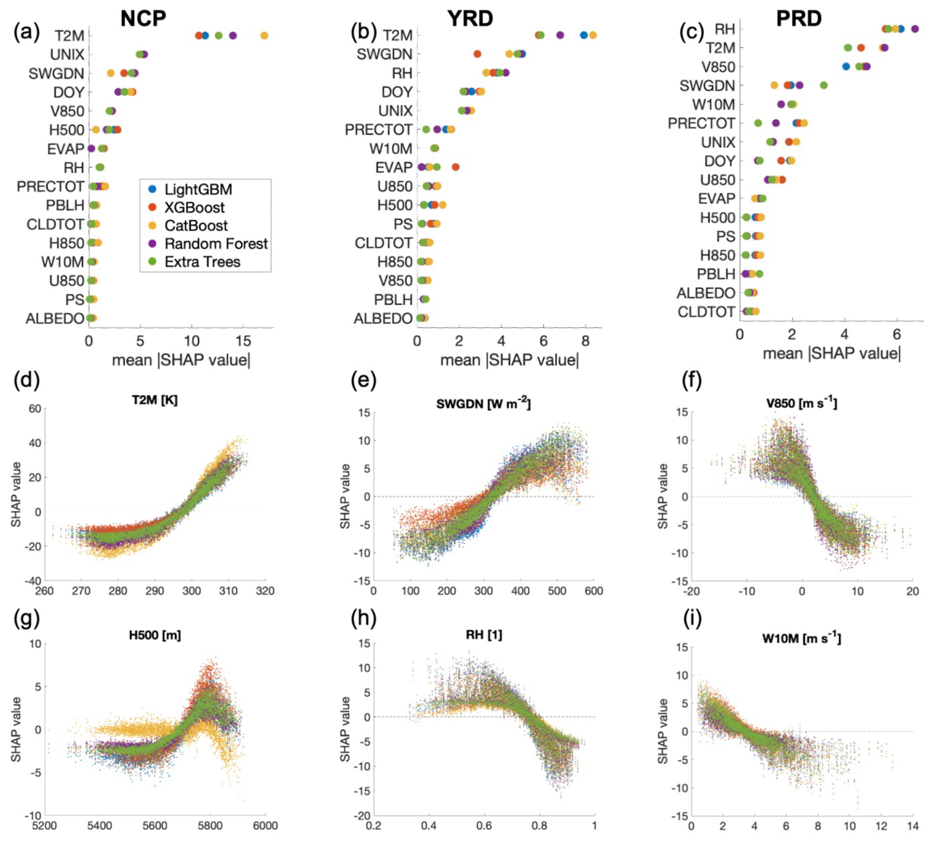
Figure 2 (a–c) Global feature importance for the three regions: North China Plain (NCP, left column), Yangtze River Delta (YRD, middle column), and Pearl River Delta (PRD, right column), calculated by averaging the absolute SHAP values across all days. (d–i) Scatter plots of selected meteorological variables versus their SHAP values, illustrating local explainability. Each point represents a daily observation, and different colors correspond to different ML models.

Figure 2d–i show scatter plots of individual meteorological variables against their SHAP values, providing local explainability insights for each region. Here, positive (negative) SHAP values indicate that the feature value increases (decreases) the predicted ozone concentration relative to the baseline expectation (C in Eq. 1). Two key variables are highlighted per region, with additional examples shown in Figs. S4–S6. Overall, the ozone–meteorology relationships revealed by XML are consistent with established physical understanding. For instance, surface ozone levels are positively correlated with T2M and SWGDN, and negatively correlated with RH and W10M (Wang et al., 2017; Lu et al., 2019; Archibald et al., 2020; Fu and Tian, 2019). V850 exhibits opposite effects in NCP and PRD (Fig. S4 vs. S6). In NCP, southerly winds (V850 >0) tend to transport polluted air masses northward, worsening ozone pollution, whereas in PRD, they typically bring cleaner marine air, mitigating ozone levels. The SHAP results also uncover important nonlinear relationships. For example, the O₃–T2M relationship in NCP flattens at lower temperatures, indicating that temperature has a weaker effect on ozone variability in cold seasons than in summer. High 500 hPa geopotential height (H500) is generally associated with elevated ozone due to stable atmospheric conditions; however, beyond 5800 m, its contribution diminishes, likely due to enhanced precipitation and humidity (Fig. S7). Furthermore, the SHAP-derived O₃–V850 (Fig. 2f) and O₃–RH (Fig. 2h) relationships exhibit a two-mode pattern that varies with temperature (Fig. S8), suggesting distinct meteorological influences in summer vs. winter.

We observe considerable discrepancies in feature attribution across the five ML models. As shown in Fig. 2, although the ranking of key predictors is broadly consistent (e.g., T2M is the leading predictor in NCP), the magnitudes of SHAP values vary substantially across models, leading to uncertainty in their quantitative importance. One illustrative example is the sensitivity of ozone to temperature ($\mathrm{d}{\mathrm{O}}_{\mathrm{3}}/\mathrm{d}T$), a key metric for assessing the ozone climate penalty (Bloomer et al., 2009; Jaffe and Zhang, 2017). We estimate $\mathrm{d}{\mathrm{O}}_{\mathrm{3}}/\mathrm{d}T$ by fitting a linear regression between summertime SHAP values and T2M values (Fig. 2d). Across the five models, $\mathrm{d}{\mathrm{O}}_{\mathrm{3}}/\mathrm{d}T$ estimates range from 1.74 to 2.70 ppbv K⁻¹ in NCP, 0.81 to 1.27 ppbv K⁻¹ in YRD, and 0.80 to 1.43 ppbv K⁻¹ in PRD (Table S2). These inter-model variations are comparable to the spread observed in previous process-based modeling studies (Chen et al., 2024; Porter and Heald, 2019; Zhang et al., 2022), underscoring the importance of model choice when interpreting climate sensitivity estimates.

These discrepancies in explainability are likely driven by multicollinearity among input features. As shown in the correlation heatmap (Fig. S1), T2M is highly correlated with SWGDN, H500, surface pressure (PS), and evaporation (EVAP) in all three regions. Different ML algorithms assign varying importance to these correlated features. For example, in NCP, CatBoost attributes the highest global importance to T2M and the lowest to SWGDN and H500 compared with other algorithms (Fig. 2a). This is also reflected in CatBoost's SHAP values for H500, which are near zero when H500 is below 5700 m (Fig. 2g). We further conduct a sensitivity experiment in which SWGDN, H500, PS, and EVAP are excluded from the input features (Fig. S9). However, inter-model discrepancies persist, primarily due to strong collinearity between T2M and DOY (Fig. S1). Removing DOY reduces these discrepancies but degrades performance across all five models. Since our goal is to use XML to reveal underlying physical relationships, we prioritize retaining a comprehensive set of relevant features, even if some are correlated and may lead to overfits, so that subtle but important processes can be kept (e.g., ozone responses to H500 or SWGDN) (Jiang et al., 2024).

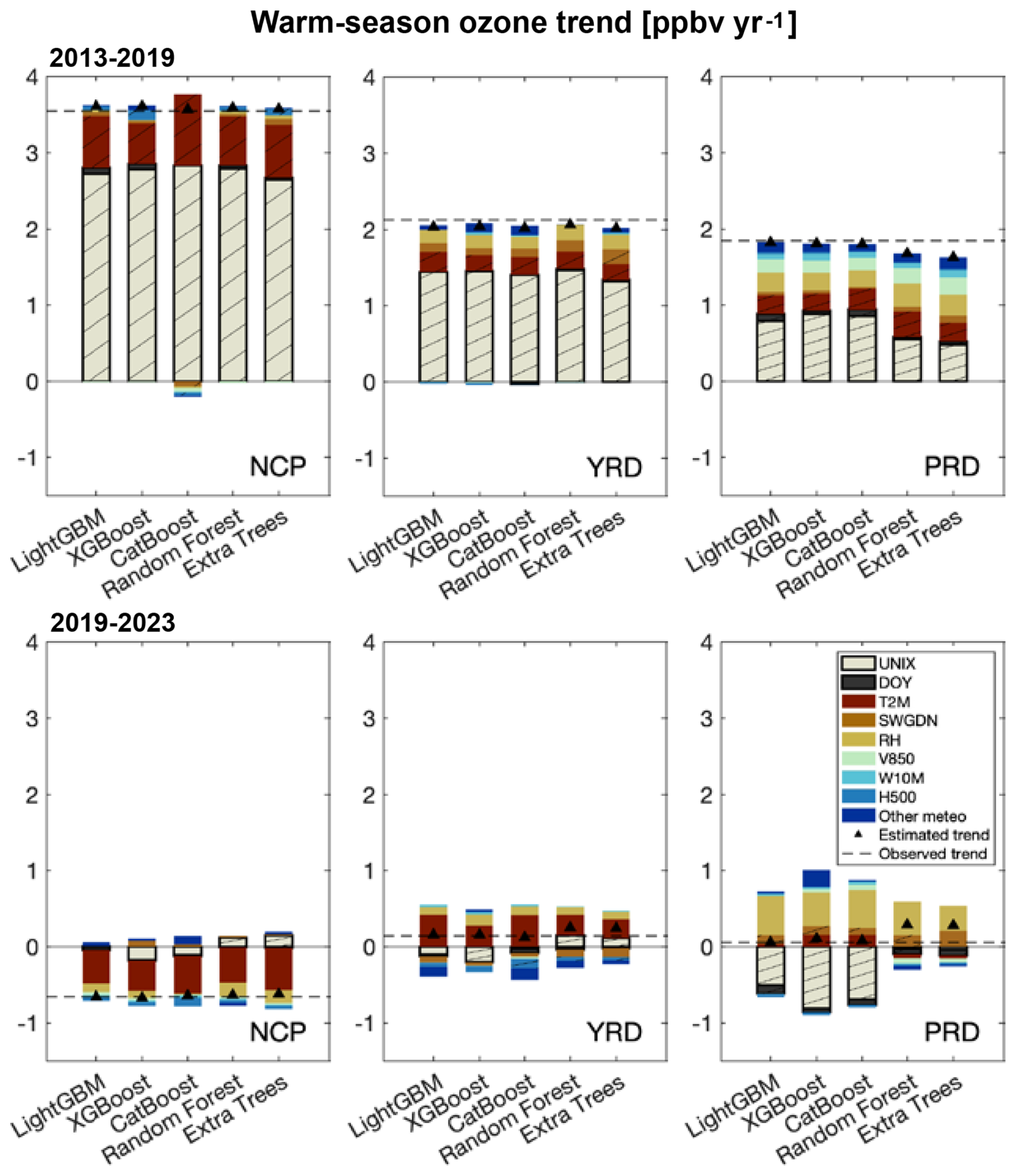
Figure 3 Attribution of warm-season (April to September) surface ozone trends to meteorological and temporal variables for the periods 2013–2019 (top panels) and 2019–2023 (bottom panels) in three Chinese regions (NCP, YRD, and PRD). Results from the five ML models (LightGBM, XGBoost, CatBoost, Random Forest, and Extra Trees) are presented as individual bars, with colors representing contributions from specific meteorological and temporal (UNIX and DOY) variables. Hatches denote statistically certain trends (p<0.05).

3.2 The impacts of meteorology on surface ozone trends over 2013–2023

We assess the contribution of meteorology to long-term ozone trends by calculating linear trends in warm-season (April–September) SHAP values for each input variable using a parametric regression method (Lu et al., 2020). We divide the study period into two phases (pre-2019 and post-2019) since 2019 marks a turning point in the ozone trend, transitioning from rapid increases to stabilization or decline (Fig. 3). SHAP values enable attribution of observed ozone trends to individual meteorological variables and two temporal features. DOY captures the seasonal cycle, and UNIX reflects non-meteorological influences such as emission changes (see Sect. 2.3). The observed warm-season ozone trends (dashed line in Fig. 3) are 3.5, 2.1, and 1.8 ppbv yr⁻¹ for NCP, YRD, and PRD, respectively, before 2019, and −0.66, 0.14, and 0.06 ppbv yr⁻¹ after 2019. The five ML models reproduce these trends reasonably well, with some discrepancies, particularly in PRD, where Random Forest and Extra Trees underestimate the pre-2019 increase and overestimate the post-2019 trend.

We find that meteorological and non-meteorological factors show contrasting roles in shaping surface ozone trends before and after 2019. In NCP and YRD, all five ML models indicate that the UNIX variable accounts for over half of the 2013–2019 ozone increases, whereas its influence is weak during 2019–2023, when meteorological factors become the primary drivers. In PRD, results from LightGBM, XGBoost, and CatBoost indicate that the UNIX term explains nearly 46 % of the pre-2019 ozone increase but shifts to a negative influence after 2019, offsetting the positive effects of meteorology. By contrast, Random Forest and Extra Trees attribute only ∼28 % of the pre-2019 ozone rise to the UNIX term and show almost no influence over 2019–2023, reflecting weaker ozone–UNIX relationships in these models (Fig. S6). These findings align with previous studies showing that China's clean air actions contributed to rising ozone levels during Phase 1 (2013–2017) but led to slight declines during Phase 2 (2018–2020) as coordinated controls of NMVOCs and NO_x were implemented (Liu et al., 2023; Wang et al., 2023). Our XML results support these findings, demonstrating that the UNIX variable, a proxy for non-meteorological influences such as emissions, plays distinct roles in the evolution of ozone concentrations before and after 2019.

We analyze the influence of specific meteorological variables on ozone trends using SHAP values. Temperature (T2M) is the most critical factor before 2019, with all five ML models consistently identifying its significant contribution to ozone trends (p<0.05) across the three regions. In NCP, temperature is particularly important, contributing to ozone increases of 0.53–0.93 ppbv yr⁻¹ across models during 2013–2019, followed by ozone declines after 2019. Such shifts in meteorological influences around 2019 in NCP have also been reported in a recent study that attributed them to reversed changes in meteorological variables (Wang et al., 2024). In YRD, the combined effects of temperature, solar radiation, and humidity contribute to ozone increases of ∼0.54 ppbv yr⁻¹ during 2013–2019. After 2019, although changes in temperature and humidity moderately enhance ozone levels, their effects are largely offset by other meteorological variables. In PRD, temperature, humidity, and wind conditions (V850 and W10M), along with other meteorological factors, collectively enhance surface ozone before 2019, whereas RH becomes the primary driver of ozone increases afterward.

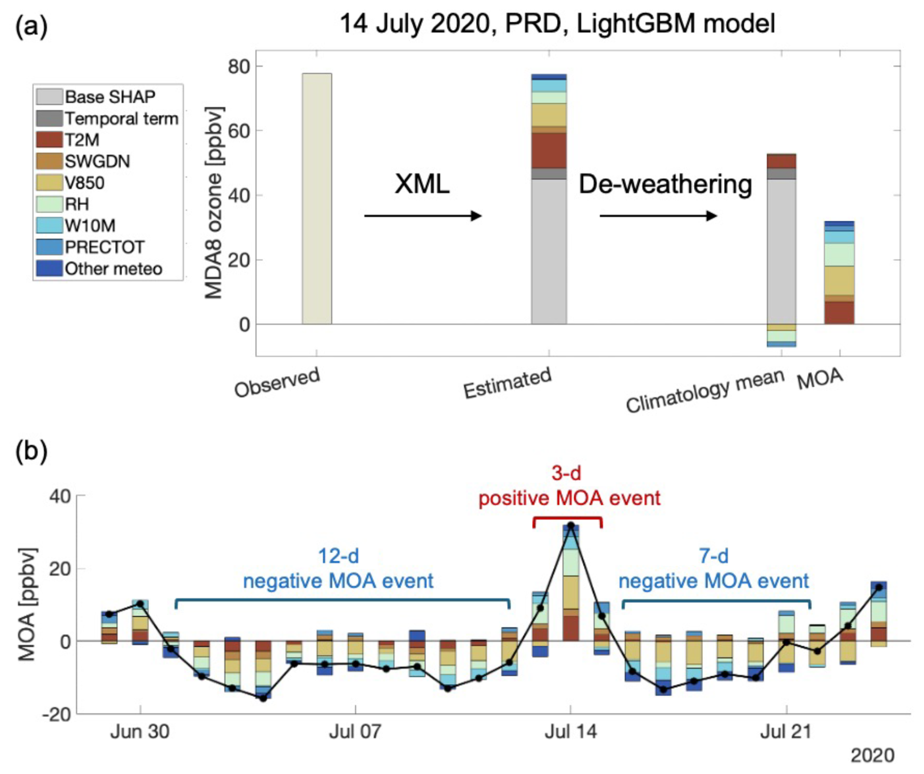
Figure 4 Schematic diagram of the attributable de-weathering approach, using an event of 14 July 2020 in the PRD region as diagnosed by the LightGBM model. (a) Steps for deriving the climatological mean ozone and the meteorology-induced ozone anomaly (MOA) on 14 July 2020. (b) MOA values in PRD from 29 June to 24 July 2020, with identified MOA events highlighted.

3.3 Meteorology-induced ozone anomaly

We now apply the attributable de-weathering approach described in Sect. 2.3 to decompose daily ozone into a climatological mean and meteorology-induced ozone anomaly (MOA). Figure 4a shows a pollution event in PRD, with regional mean surface ozone peaking on 14 July 2020. The observed MDA8 ozone reached 77.6 ppbv on 14 July 2020, while the five ML models estimated similar values ranging from 76.4 to 77.5 ppbv (only the LightGBM result is shown for clarity). After de-weathering, the climatological ozone level is estimated to be ∼45 ppbv. Several meteorological variables, such as RH, V850, and PRECTOT, negatively contribute to this climatology, reflecting the influence of 15 d running averages (Eq. 3) in mid-July. Subtracting it from the total ozone yields the MOA being as high as 32 ppbv on that day. All five models identify V850 as the most influential meteorological factor, accounting for about one-third of the MOA. Additional important factors include RH, T2M, PRECTOT, SWGDN, and 10 m wind speed (W10M), all enhancing the MOA during this pollution event (Fig. 4b). We note that extreme ozone events may also be influenced by non-meteorological factors (e.g., emission pulses or regional transport of precursors), which are captured by the UNIX term in our framework but are not included in the MOA calculation. Therefore, MOA should be interpreted as the meteorologically driven component of ozone anomalies, rather than a comprehensive representation of all extreme ozone events.

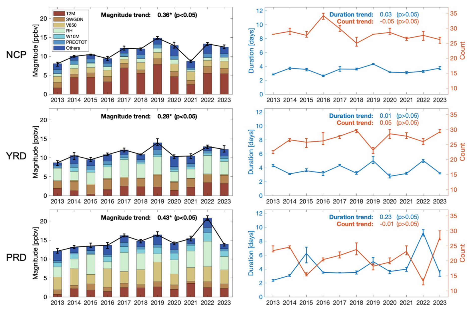
Figure 5 Left column: Magnitude of positive MOA events during warm seasons from 2013 to 2023 for NCP (top), YRD (middle), and PRD (bottom). Bars represent contributions from individual meteorological variables. Trends in unit of ppbv/year are shown inset. Right column: Duration and count of positive MOA events over the same period. Results are averaged across five ML models, with error bars indicating the range among models.

We focus on positive MOA events during warm seasons, and calculate the average magnitude and duration for each event (e.g., Fig. 4b). Figure 5 shows their interannual variations and trends from 2013 to 2023. Averaged across five ML models, the mean magnitudes of positive MOA values are 11.7 ppbv in NCP, 11.5 ppbv in YRD, and 15.9 ppbv in PRD (Table S3). Our analysis reveals significant increasing trends (p<0.05) in MOA magnitude across all three regions, with annual rates of 0.36, 0.28, and 0.43 ppbv yr⁻¹ in NCP, YRD, and PRD, respectively. After 2019, the magnitude of MOA events becomes more variable. For instance, in 2021, MOA values in NCP were notably low, mainly due to the reduced T2M influences. In contrast, PRD experienced a sharp peak in MOA in 2022, reaching nearly 20 ppbv, largely driven by decreased RH. Figure S10 compares the global importance of original SHAP values with those based on anomalies. In NCP, although T2M is less dominant in anomaly-based importance compared to the original ranking, it remains the most influential factor in explaining ozone anomalies. In YRD, the importance of temperature drops from first in the original ranking to third in the anomaly-based ranking, where it contributes comparably to RH and SWGDN. Moreover, the relative importance of V850 increases in both NCP and PRD, indicating enhanced influence of synoptic-scale transport on daily ozone variability.

In contrast to the increasing trend in MOA magnitude, none of the five ML models indicates significant trends in the duration of MOA events over the study period (Fig. 5). However, the MOA duration in PRD shows notable interannual variability. On average, positive MOA events last 3.1 d in NCP, 3.4 d in YRD, and 4.3 d in PRD. Notably, a prolonged positive MOA event lasting over 30 d was recorded in PRD from 27 August to 26 September 2022. XML results suggest that this event was mainly driven by sustained anomalies in RH, T2M, and V850 (Fig. S11). The extended duration of positive MOA in PRD relative to NCP and YRD may be attributed to persistent weather systems such as the subtropical high and typhoons (Chen et al., 2022; Wang et al., 2018). We also analyze the annual counts of positive MOA events and find no significant trends in any of the three regions (Fig. 5). These findings suggest that the intensified meteorological influence on surface ozone in China from 2013 to 2023 is primarily due to increasing MOA magnitudes, rather than more frequent or longer-lasting episodes of unfavorable meteorological conditions.

4 Conclusions and uncertainty analyses

In summary, we have applied the SHAP technique to the outputs of five ML models to analyze the impact of meteorology on surface ozone in three Chinese regions. All five models consistently identify important meteorological drivers of ozone variability, including temperature, solar radiation, humidity, wind, and geopotential height. The XML results also reveal their nonlinear relationships with ozone, which generally align well with established physical understanding. Our results highlight a temporal shift in the dominant drivers of ozone trends over the past decade. During the early phase of China's clean air actions (prior to 2019), rising ozone levels were largely attributed to emission changes, while in the later phase (post-2019), meteorological variability become prominent. Among meteorological factors, temperature is identified as the most influential variable, with significant contributions to pre-2019 ozone trends in all three regions across all five models. Furthermore, the SHAP-based de-weathering approach shows a clear increase in the magnitude of positive meteorology-induced ozone anomaly (MOA) events in recent years.

Our work highlights not only the valuable insights that XML can offer but also the potential challenges associated with its application to ozone attribution and broader environmental analysis. One major challenge is the presence of multicollinearity among meteorological variables, which complicates the interpretation of individual variable contributions. Machine learning models may arbitrarily assign higher importance to one correlated variable over another, leading to potentially misleading conclusions. This issue is particularly relevant when using XML outputs for policy-relevant assessments, such as estimating the ozone climate penalty (i.e., $\mathrm{d}{\mathrm{O}}_{\mathrm{3}}/\mathrm{d}T$). More broadly, the collinearity among input variables can introduce uncertainty in explaining the relative importance of different drivers. In our case, only the UNIX and DOY terms are included as non-meteorological indicators due to their weak correlations with meteorological variables (Fig. S8). However, incorporating additional inputs, such as concentrations of other pollutants, would likely increase the model's complexity and hinder interpretability. It is also noted that systematic differences in meteorological reanalysis products for certain variables may influence the relative importance assigned to predictors. For instance, Lu et al. (2025) reported discrepancies in surface shortwave radiation between MERRA-2 and ERA5 over eastern China, potentially affecting radiation-related attributions. While our conclusions regarding the dominant role of temperature remain robust, future studies could benefit from multi-reanalysis ensembles to quantify this uncertainty.

Second, inconsistencies in XML results may arise from two sources: variations in feature attributions across different models and differences in the models' predictive performance. Disentangling these two sources of uncertainty is inherently difficult. For instance, in our study, the contribution of the UNIX variable to ozone trends in PRD, as identified by Random Forest and Extra Trees, differs significantly from that identified by the other algorithms (Fig. 3). This discrepancy could be due to weaker modeled relationships between ozone and UNIX in the two models, larger biases compared to observational data, or a combination of both factors. In practice, models with higher predictive performance tend to provide more reliable explanations identifying the key features.

Finally, our analyses rely exclusively on the SHAP technique due to its ability to provide local explainability information. However, the use of alternative XML methods may introduce additional layers of uncertainty in interpretation. For example, Table S4 compares global feature importance rankings generated by three different XML approaches, SHAP, Gain, and Permutation, for the LightGBM model. The inconsistencies among these importance rankings suggest that only general features, such as which variables are influential and which are not, can be reliably inferred. This highlights the need for future work to develop standardized evaluation metrics that can help distinguish more reliable and consistent explanations from the diverse outputs of multiple XML methods, such as those evaluated by Krishna et al. (2022).