An improved high-resolution passenger vehicle emission inventory for China using ride-hailing big data

As the global automotive industry continues to grow rapidly, the increasing number of passenger vehicles has contributed to worsening air pollution. However, previous studies have insufficiently addressed nationwide hourly vehicle emissions. This study firstly utilized big data of ride-hailing services and traffic flow model to obtain nationwide hourly gridded speed and traffic volume. Then we established a high spatiotemporal resolution (0.01° × 0.01°; 1 h) emission inventory by using multiple correction factors. The annual amounts of CO, VOCs, NO_x, PM and NH₃ emitted from national passenger vehicles in 2019 were 4087.8, 1069.4, 211.7, 1.9, 77.5 kt, respectively. Despite occupying merely 0.8 % of the national territory, urban areas generated 35.3 % of the country's total vehicle emissions, due to high local traffic volumes and relatively low vehicle speeds. From a temporal perspective, passenger vehicle emissions exhibit significant holiday effect and weekend effect. In addition, hourly average emissions on workday exceeded those of weekend and holiday by 8 % and 5 % during the morning peak, with these differences increasing to 12 % and 18 % during the evening peak. Current traditional emission methodology might underestimate emissions by 31.5 %. We also used the WRF-Chem model for simulation validation. This hourly-scale inventory provides quantitative support for the precise implementation of pollution control and early warning.

1 Introduction

The number of vehicles in China grew from 14.53 million to 260 million over the past two decades, with an average annual growth rate of 16.39 % (MEE, 2020). This growth has driven economic development while adversely impacting air quality and human health (Anenberg et al., 2017). Premature deaths attributable to PM_2.5 in China amounted to 1.33 million in the year 2020, of which motor vehicle emissions contributed approximately 12.5 % (Li et al., 2023b; Luo et al., 2022). In 2019, passenger vehicles accounted for about 80 % of the total vehicle population in China (NBS, 2020) and contributed significantly to vehicular emissions (e.g., VOCs accounted for more than 50 % of the total) (Li et al., 2023a). Quantification of passenger vehicle emission characteristics is imperative for the evaluation of relevant emission reduction policies.

With the advancement of regional air quality simulation technology and the increasing demand for atmospheric environmental management, traditional traffic emission statistical methods have become inadequate to meet current refined management requirements (Gao et al., 2020). To address this issue, previous studies have developed numerous methods for constructing refined vehicle emission inventories. The first category involves constructing high spatiotemporal resolution traffic emission inventories by using complex emission models, such as COPERT, MOVES, and IVE (Yang et al., 2018; Yu et al., 2021; Latini et al., 2005; Huo et al., 2009). For example, Dey et al. (2019) estimated the emission levels of 8 types of pollutants from passenger cars in the Greater Dublin Area of Ireland based on the COPERT5 model. The second category utilizes big data on transportation. For instance, Dias et al. (2018) improved the characterization of the spatial variation of vehicle speeds at the city scale through GPS modeling, and Deng et al. (2020) utilized the BeiDou Navigation Satellite System (BDS) to establish an emission inventory with lower uncertainty for the Beijing-Tianjin-Hebei (BTH) region. Yeganeh et al. (2025) quantified the high-resolution spatiotemporal characteristics of traffic-related PM_2.5 and black carbon (BC) using long-term mobile monitoring data collected along five representative routes in Tehran, Iran. However, due to the difficulties in obtaining large-scale and long-term traffic data, most studies are also limited to roads, cities or urban agglomerations, such as Chengdu, Beijing, and the Pearl River Delta (PRD) (Li et al., 2020c; Zheng et al., 2009; Wen et al., 2022), for emission calculations. There is a lack of hourly-resolution emission estimates at the national level.

Emission factors are generally considered to be one of the primary sources of uncertainty in emission inventories (Charis et al., 2010). Many scholars focus merely on the impact of vehicle technology improvements, fuel types, and vehicle aging on emission factors, while often neglecting the influence of speed (Xu et al., 2021; Kean et al., 2003). Speed has the greater impact on emission factors compared to other correction factors, as it fluctuates dynamically within the same region, while other correction factors remain relatively constant over time. This difference is primarily attributed to variations in engine workload and combustion efficiency at different speeds (Sun et al., 2020; Kean et al., 2003). The impact of speed on vehicle emissions is both significant and complex. For NO_x, the emission rate of light-duty passenger vehicles at high speeds (>50 km h⁻¹) is 1.6 times that at low speeds (10–20 km h⁻¹), while the emission rates of HC and CO at low speeds are 1.6 times and 2.3 times that of high-speed driving, respectively (Guo et al., 2020). Given this impact, accurate calculation of speed correction factors is important for reducing the uncertainty of emissions factors.

The temporal allocation method can also directly affect the accuracy of high-resolution emission inventories. Previous studies have established emission inventories at monthly scales (Zheng et al., 2014; Jiang et al., 2020; Zhou et al., 2017), or roughly obtained daily-scale data, followed by the construction of a regional-level hourly-scale inventory, such as Biswal et al. (2022), who systematically analyzed hourly gridded road traffic emissions in Delhi city; Sun et al. (2021), who considered the influence of the vehicle age-annual average mileage curve and estimated hourly emissions on a 0.01° × 0.01° grid in Tianjin. However, they have ignored the fluctuations in daily emissions caused by workday, weekend, and holiday, which has significant uncertainty.

To address these gaps, this study aims to improve the accuracy of emission estimations by utilizing big data of ride-hailing services to obtain nationwide speed distribution on a 0.01° grid for the first time and apply it to the speed correction of emission factors. We construct a high spatiotemporal resolution (0.01° × 0.01°; 1 h) emission inventory of atmospheric pollutants from passenger vehicles in China in 2019 by further integrating traffic flow models and big data of the congestion delay index. The study also explores the spatiotemporal characteristics of pollutant emissions from passenger vehicles, compares the results with traditional calculation methods, and further evaluates the inventory improvement using WRF-Chem model.

2 Data and methodology

2.1 Estimation of emission inventories

The emission inventory for each pollutant (CO, VOCs, NO_x, PM, NH₃) for passenger cars was estimated with the following equation:

$$\begin{array}{}\text{(1)}& {\displaystyle }\begin{array}{rl}{E}_j& =\sum _{i,p,k,t}{V}_{p,i,k,t}\times {\mathrm{BEF}}_{p,j}\times {\mathit{\phi }}_{p,i,j,t}\times {\mathit{\gamma }}_{p,i,t}\\ & \times {\mathit{\lambda }}_{p,j}\times {\mathit{\theta }}_{p,j}\times {\mathrm{10}}^{-\mathrm{9}}\end{array}\text{(2)}& {\displaystyle }{V}_{p,i,k,t}={\mathrm{VP}}_{p,i,k,t}\times {\mathrm{VKT}}_{p,i,t}\text{(3)}& {\displaystyle }\mathrm{TPEs}=\sum _j{\displaystyle \frac{E_j}{{\mathrm{PEV}}_j}}\end{array}$$

In Eqs. (1) and (2), E represents pollutant emissions (t); i represents the grid; j represents the pollutant type, including CO, PM, VOCs, NO_x and NH₃; k represents the vehicle type, including small passenger cars and mini passenger cars; p represents the province; VP, VKT, and BEF represent the vehicle population, annual average vehicle kilometers traveled and baseline emission factors, with units of vehicles, km yr⁻¹, and g km⁻¹, respectively. φ is the environmental correction factor (including temperature correction factor, humidity correction factor, and altitude correction factor); γ is the speed correction factor; λ is the deterioration correction factor; θ represents other correction factors (including sulfur content correction factor and ethanol blending correction factor). In Eq. (3), TPEs represents the total pollutant equivalents (kt) (For assessing the extent of environmental and techno-economic hazards posed by various pollutants), and PEV represents the pollutant equivalent value (kg) (MEE, 2018). This study focused on gasoline-fueled passenger vehicles. The vehicle kilometers traveled (VKT) of light-duty gasoline passenger vehicles (LDPVs) in 2019 were obtained from Ma et al. (2022). Based on the China Statistical Yearbook 2004–2019, we calculated the proportion of passenger vehicles by emission standard, the total number of passenger vehicles in each province in 2019 (Fig. S1 in the Supplement), and the regional distribution of small and mini passenger vehicles by emission standard (Fig. S2). The baseline emission factors were obtained based on other literature (Wen et al., 2023; MEE, 2014; EEA, 2019), with specific details provided in Table S1 in the Supplement. Furthermore, the definition of urban and rural areas involved in this study was based on the research of Li et al. (2020b).

The core difference between the traditional algorithm and the improved algorithm in this study was that the former assigned a fixed speed correction factor for each of the five speed intervals with monthly-scale activity levels, while the latter obtained continuous speed correction factors and further refined the activity levels by combining the congestion index with the traffic flow model. The detailed correction values could be found in Table S2.

2.2 Quantification of high-resolution emission factors based on big data of ride-hailing

2.2.1 Gridded speeds and determination of their correction factors

A total of 23.6 billion vehicle trajectory data were collected in this study from Amap Ride-hailing Platform (https://lbs.amap.com/, last access: 27 April 2026), including workdays (24 September, 23 October 2019), weekends (28 September, 26 October 2019) and holidays (13 September, 1 October 2019) (Table S3). The platform data originates from mobile terminal users who have activated GPS positioning. The data uploading behavior is primarily associated with the activation status of the positioning function and has no direct connection with vehicle age. This dataset had covered all major road types nationwide. To address the insufficient sample size of ride-hailing services in Western China, we adopted the nearest neighbor interpolation method to supplement the speed information of road segments with missing values across each road type. Moreover, we assumed that the vehicle speeds on other dates did not vary significantly compared to these representative days, and that passenger vehicles have consistent on-road driving speeds. Each vehicle sent data every 3 s. Using Python, we processed the data to obtain hourly resolution vehicle speeds on a 0.01° grid. Finally, we obtained gridded hourly vehicle speeds for three representative days: workdays, weekends, and holidays.

Furthermore, we adopted the improved speed correction curve (SCC) method proposed by Sun et al. (2020) to obtain continuous speed correction factor values for VOC, NO_x, and CO, ultimately resulting in gridded speed correction factors. For specific SCC of various pollutants, please refer to Table S4.

2.2.2 Corrections for other emission factors

In the equations, φ utilizes daily temperature, humidity, and elevation data, all obtained from ERA5 (https://cds.climate.copernicus.eu/datasets, last access: 27 April 2026). The deterioration correction factor λ is calculated using relevant equations and coefficients from the EEA (2019). θ includes the sulfur content correction factor and the ethanol blending correction factor, which are based on the corresponding values from GEI (MEE, 2014). Specific values can be found in Table S5.

2.3 High-resolution vehicle activity level data combined with traffic flow models

For time allocation for vehicle activity levels, the following formula can be used:

$$\begin{array}{}\text{(4)}& V_{p,t,k}=C_{p,t}\times V_{p,k}=C_{p,t}\times {\mathrm{VP}}_{p,k}\times \mathrm{VKT}\end{array}$$

where $V_{p,t,k}$ is the vehicle activity level of model k in province p in time period t (vkm); V_p,k is the number of vehicles of model k in province p (vkm).

C_p,t is the time allocation coefficient of province p at time period t. It is obtained by combining the congestion delay index obtained from Baidu Map Traffic and Travel Big Data Platform (https://jiaotong.baidu.com/, last access: 27 April 2026) with the three-parameter model of traffic flow (Wang et al., 2024), which is constructed as follows:

The congestion delay index (λ) is defined as the ratio of the actual time spent by residents on one trip to the time spent in a smooth state when the travelling distance is the same, and its calculation formula is:

$$\begin{array}{}\text{(5)}& \mathit{\lambda }={\displaystyle \frac{T}{T_f}}={\displaystyle \frac{\frac{L}{v}}{\frac{L}{v_f}}}={\displaystyle \frac{v_f}{v}}\end{array}$$

Where, λ is the congestion delay index, dimensionless; T is the actual time spent travelling (h); T_f is the time spent travelling at the smooth speed (h); L is the length of the road section (km), v is the actual travelling speed (km h⁻¹), and v_f is the smooth speed of the vehicle (km h⁻¹), then:

$$\begin{array}{}\text{(6)}& v={\displaystyle \frac{v_f}{\mathit{\lambda }}}\end{array}$$

Combined with the basic three-parameter model of traffic flow, the relationship between flow rate and congestion index can be derived:

$$\begin{array}{}\text{(7)}& Q=K_j\left(v-{\displaystyle \frac{v^{\mathrm{2}}}{v_f}}\right)=K_j\left[{\displaystyle \frac{v_f}{\mathit{\lambda }}}-{\displaystyle \frac{{\left(\frac{v_f}{\mathit{\lambda }}\right)}^{\mathrm{2}}}{v_f}}\right]=K_j{v}_f{\displaystyle \frac{\mathit{\lambda }-\mathrm{1}}{{\mathit{\lambda }}^{\mathrm{2}}}}\end{array}$$

Where Q is the flow rate (veh h⁻¹); λ is the congestion delay index; K_j is the congestion density (veh km⁻¹); v_f is the unimpeded vehicle speed, and K_j and v_f are constants.

In turn, we obtain the formula for calculating the time allocation coefficient of motor vehicle emissions:

$$\begin{array}{}\text{(8)}& C_t={\displaystyle \frac{Q_t}{\sum _{\mathrm{1}}^t{Q}_t}}={\displaystyle \frac{K_j{v}_f\frac{{\mathit{\lambda }}_t-\mathrm{1}}{{\mathit{\lambda }}_t^{\mathrm{2}}}}{{\sum }_{\mathrm{1}}^t{K}_j{v}_f\frac{{\mathit{\lambda }}_t-\mathrm{1}}{{\mathit{\lambda }}_t^{\mathrm{2}}}}}={\displaystyle \frac{\frac{{\mathit{\lambda }}_t-\mathrm{1}}{{\mathit{\lambda }}_t^{\mathrm{2}}}}{\sum _{\mathrm{1}}^t\frac{{\mathit{\lambda }}_t-\mathrm{1}}{{\mathit{\lambda }}_t^{\mathrm{2}}}}}\end{array}$$

Where C_t is the motor vehicle emission time allocation coefficient, dimensionless; t is time; and Q_t denotes the volume of traffic in time period t.

Regarding the spatial allocation of the vehicle activity level, this study was done using the road length data provided by Golder Maps as an allocation index (Gómez et al., 2018), and the gridded vehicle activity level at 0.01° × 0.01° resolution was calculated according to the following formula:

$$\begin{array}{}\text{(9)}& V_{p,i,k,t}={\displaystyle \frac{L_{p,i}}{\sum _i{L}_{p,i}}}\times V_{p,t,k}\end{array}$$

where $V_{p,i,k,t}$ is the activity level of model k in the i grid of province p in time period t; $V_{p,t,k}$ is the number of vehicles of model k in province p in time period t; and L_p,i is the length of the road in the i grid of province p (km).

2.4 WRF-Chem model setting

To verify the superiority of the improved inventory, this study employed the WRF-Chem model to simulate the atmospheric concentrations of PM_2.5 and O₃ in the Jiangsu and Shanghai regions (longitude range: 117.5° E–122.0° E; latitude range: 30.0° N–35.10° N) from 1 to 18 February 2019 (covering the Spring Festival period and the subsequent week). A two-layer nested model with spatial resolutions of 9 × 9 km and 3 × 3 km, respectively, was adopted for the simulation. The specific simulated region is illustrated in Fig. S4a.

The inventory developed in this study was used as the input data for traffic sources, while data from the ABaCAS database was adopted for other emission sources; these two sets of data were jointly utilized to generate the anthropogenic emission files required for the WRF-Chem model (Li et al., 2023a). The 1° × 1° Final Operational Global Analysis (FNL) data provided by the National Centers for Environmental Prediction (NCEP, https://rda.ucar.edu/datasets/ds083.2/, last access: 27 April 2026) was used to obtain the initial meteorological conditions and boundary conditions. Real-time biomass burning emissions were derived from the Fire Inventory from NCAR (FINN, https://www2.acom.ucar.edu/modeling/finn-fire-inventory-ncar, last access: 27 April 2026). The global simulation results from CAM-Chem (https://www.acom.ucar.edu/cam-chem/cam-chem.shtml, last access: 27 April 2026) were employed as the initial chemical conditions and boundary conditions. The specific parameterization schemes are presented in Table S6.

This study used observational data from 114 national monitoring stations within the simulated area to comprehensively evaluate the simulation results of the emission inventory developed in this study and the traditional inventory, as well as the improvement effects at the 15 stations located in the regions with the top 20 % road density. The simulation results were verified by calculating the normalized mean deviation (NMB) and coefficient of determination (R²).

3 Results and discussion

3.1 Spatiotemporal variation of vehicle speed and traffic flow

Vehicle speed and traffic volume are important parameters for describing vehicle driving conditions and traffic flow characteristics. The nationwide average passenger vehicle speed was 42.42 km h⁻¹. The high concentration of work and business activities in the eastern China during the daytime, combined with its large vehicle population, led to generally slower vehicle speeds at 08:00 UTC+8 compared to 22:00 UTC+8 (time zone used throughout). Especially in the key cities such as Beijing, Shanghai, and Guangzhou, city vehicle speeds at 08:00 a.m. typically were 36.4 ± 0.3 km h⁻¹ due to significantly increased traffic flow during the morning peak and the circular radial road network which might concentrate traffic flow (Liu et al., 2018). During the off-peak period at 22:00, differences in traffic flow speeds across various road types were more apparent. The vehicle speeds on some provincial and county roads had increased significantly. This reflected the non-uniformity of traffic flow distribution (Guan et al., 2024).

There were also differences in average vehicle speeds between provinces, with Inner Mongolia, Jiangxi, and Qinghai having higher speeds (Fig. 1c). While Yunnan Province had the lowest average vehicle speed, which might be related to its unique topography. Approximately 94 % of Yunnan Province was mountainous, with an average elevation exceeding 2000 m (Gu et al., 2016). These complex topographical conditions influenced the actual driving speed of vehicles (Hou et al., 2019). In addition, compared to the Northeast China (NE: 08:00: 44.18 km h⁻¹; 22:00: 48.37 km h⁻¹), the average vehicle speeds in the Northwest China (NW: 08:00: 36.89 km h⁻¹; 22:00: 40.41 km h⁻¹), the East China (EC: 08:00: 39.89 km h⁻¹; 22:00: 44.56 km h⁻¹), and the South China (SC: 08:00: 40.45 km h⁻¹; 22:00: 44.16 km h⁻¹) regions were lower, due to the NE was predominantly characterized by plains, and its population and transportation network were not as dense as those in the CC and SC (Fig. 1c) (Xu et al., 2023).

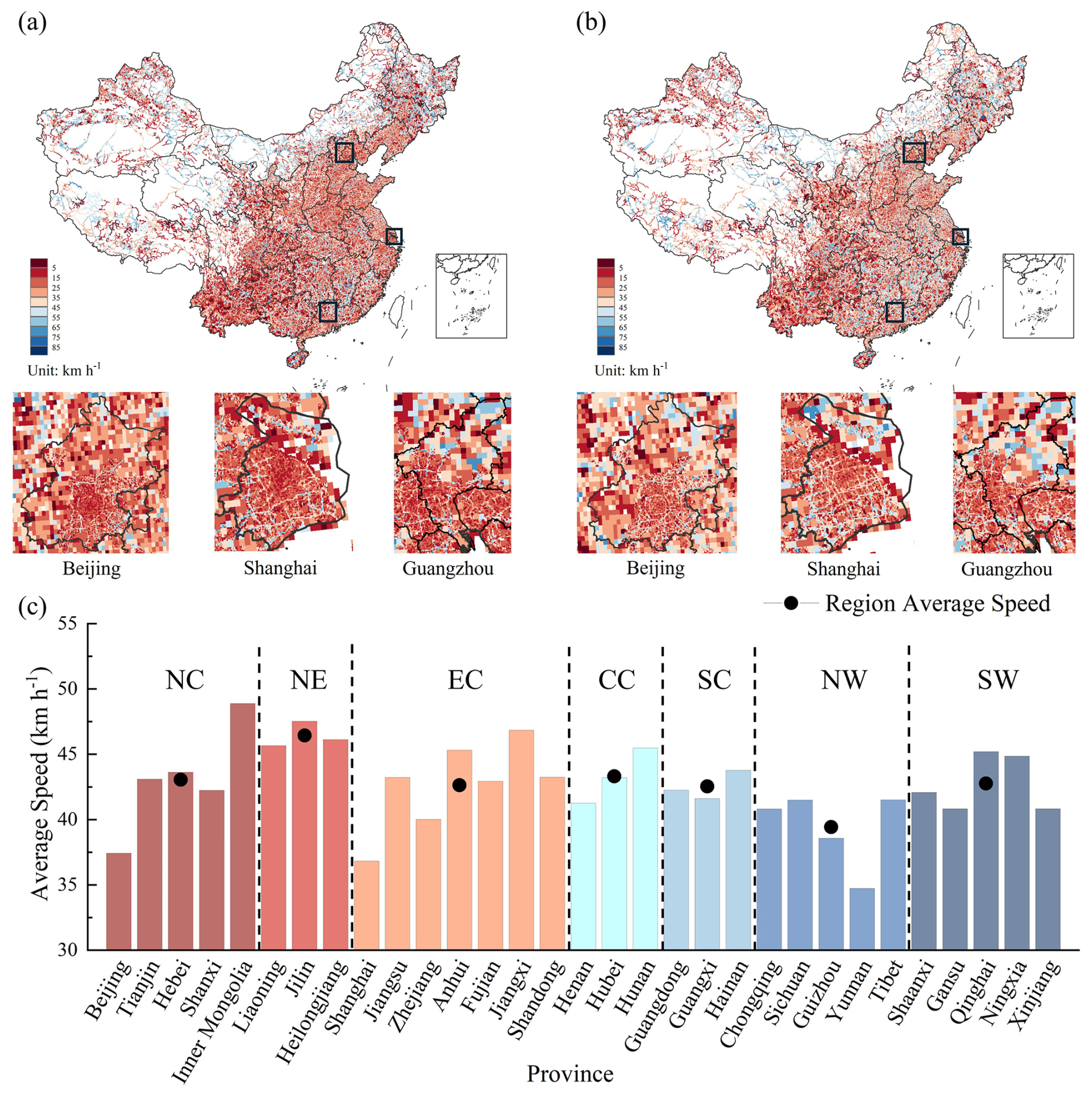
Figure 1 The average vehicle speed of passenger vehicles in China in 2019: Spatial distribution of speeds on a 0.01° grid at (a) 08:00 and (b) 22:00; (c) Average speeds of provinces and regions, where NC: North China; NE: Northeast China; EC: East China; CC: Central China; SC: South China; NW: Northwest China; SW: Southwest China.

Specific to the road type, the average driving speeds were higher on expressways (workday: 08:00: 67.12 km h⁻¹; 22:00: 68.59 km h⁻¹), urban arterial roads (workday: 08:00: 51.43 km h⁻¹; 22:00: 45.33 km h⁻¹) and national highways (workday: 08:00: 40.05 km h⁻¹; 22:00: 42.92 km h⁻¹) compared to other types of roads (Fig. 2a, b, c). Notably, urban arterial roads speeds fluctuated sharply during workdays and weekends, with fluctuation magnitudes of 25.3 and 12.8 km h⁻¹ respectively; this was attributable to the heavy intercity and interregional commuting traffic they carry, which caused a rapid surge in road saturation and thus a sharp speed drop, followed by a swift rebound (by 63.2 % and 41.2 % respectively) during midday off-peak hours as commuting demand wanes (Wang et al., 2016). By contrast, holiday travel was dominated by interregional family visits and tourism, with highly dispersed travel timings, leading to mitigated speed fluctuations across all road types. The emission factor of CO, VOCs, and NO_x all exhibited a trend of sharp decrease followed by gradual increase in response to vehicle speed, which was consistent with the combustion kinetics of internal combustion engines (Fig. 2d). Among them, the EFs of incomplete combustion pollutants (CO and VOCs) showed more significant responses to speed variations, while the EFs of thermal-generated NO_x were mainly controlled by the temperature and oxygen concentration inside the cylinder and thus showed relatively moderate responses to speed changes (Chen et al., 2022).

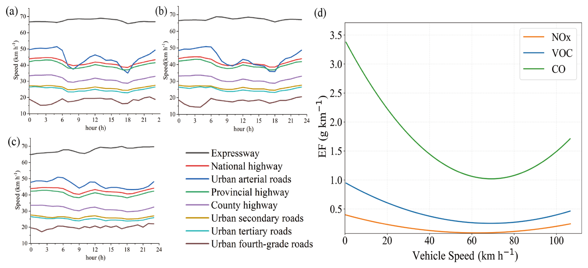
Figure 2 Temporal variations in vehicle speed on different road classes and corresponding EF-Vehicle Speed curves. Diurnal speed profiles of different road classes on (a) workday; (b) weekend; (c) holiday; (d) responses of CO, VOCs, and NO_x EF to vehicle speed.

To further quantify the impact of average vehicle speed on the model results, this study conducted a quantitative assessment of model uncertainty using Monte Carlo simulation. Across all speed intervals, the emission factors and their corresponding uncertainties for CO, VOC, and NO_x were 1.4866 ± 21.42 % g km⁻¹, 0.4042 ± 22.56 % g km⁻¹, and 0.1507 ± 28.30 % g km⁻¹, respectively. Furthermore, uncertainty analysis was performed for each speed interval. Although the 40–80 km h⁻¹ interval exhibited the lowest emission factors, it represented the dominant driving range for passenger vehicles, with the highest probability density. In contrast, the uncertainty of emission factors reached its maximum when vehicle speeds exceeded 80 km h⁻¹ (Fig. S3).

Based on ride-hailing big data, the average speed of passenger vehicles fluctuated across different times. The daily average traffic speeds on workday and weekend were consistent, with both lower than on holiday, at 42.108, 42.111, and 43.032 km h⁻¹, respectively. The higher holiday speed (Fig. 3c) can be attributed to reduced urban congestion resulting from increased public transportation use for leisure travel on holidays (Zhang and Gao, 2023b). All three-day types exhibited two low-speed valleys from 07:00–09:00 and 17:00–19:00, with the workday morning valley occurring one hour earlier compared to weekend, consistent with findings by Yang et al. (2017). The national average speed frequency distribution differed at 08:00 and 22:00 on workday (Fig. 3a and b), primarily concentrated at 34.9 ± 0.2 km h⁻¹ and 44.8 ± 0.3 km h⁻¹, respectively. Compared with weekday, there were no morning and evening rush hours on holiday, resulting in a higher proportion in high-speed intervals (Yang et al., 2016). The large difference in speed between these two periods is due to the variation in traffic volumes, as illustrated by the inverse relationship between hourly traffic volume and speed distribution (Fig. 3d).

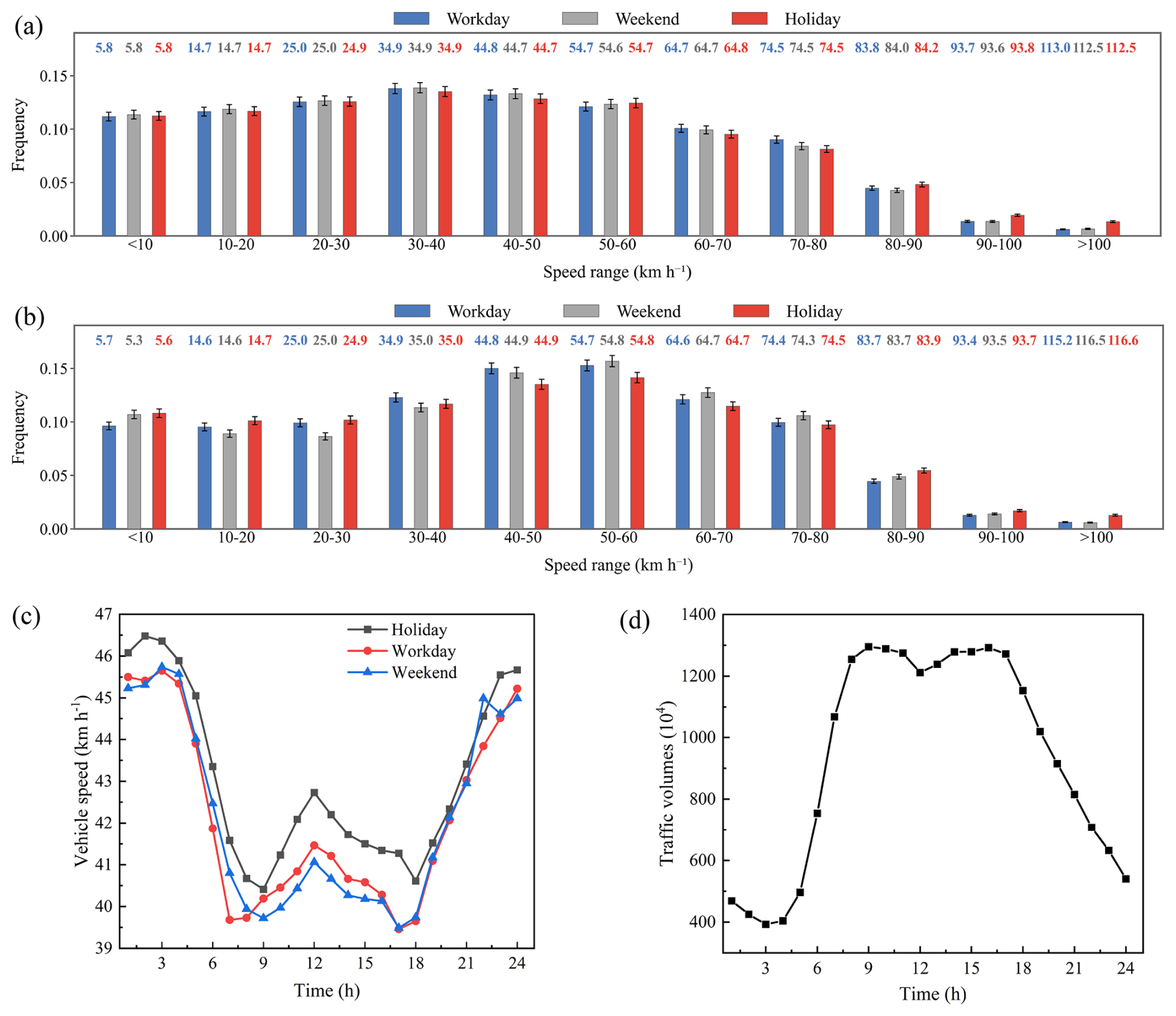
Figure 3 Characteristics of speed and traffic volume changes: speed distribution at (a) 08:00 and (b) 22:00 on workday, weekend and holiday. The values labeled in the figure represent the average speed of each interval; (c) Hourly speed variation on weekend, workday and holiday and (d) hourly traffic volume variation.

3.2 Total passenger vehicle emissions in 2019

The annual amount of CO, VOCs, NO_x, PM and NH₃ emitted from national passenger vehicles in 2019 were 4087.8, 1069.4, 211.7, 1.9, 77.5 kt, respectively and TPEs was 1.6×10³ kt. Considering these pollutants exhibited similar emission patterns, this study focused on analyzing the total pollutant equivalent emissions. Pollutant emissions from passenger vehicles showed significant spatial heterogeneity. Urban areas, despite occupying only 0.8 % of the country's total land area, accounted for a high 35.3 % of total vehicle emissions. High-pollution areas mainly concentrated in four urban agglomerations (BTH, YRD, PRD, SCB) (Fig. 4a). These areas were densely populated with high vehicle usage frequency, contributing significantly to the total emissions at 48.54 %. Specific emissions by province are shown in Table S7. The urban emission density of vehicles within four urban agglomerations was significantly higher compared to rural areas (Fig. 4b), as most passenger vehicles primarily operated in urban (Loder et al., 2019). However, variations in urban-rural vehicle ownership and land area across different urban agglomerations led to different urban-rural emission density gaps (Zhao and Bai, 2019). Notably, the Beijing-Tianjin-Hebei (BTH) urban agglomeration exhibited the largest urban-rural emission density ratio of 16.4, which was 13.5 higher than the national average. This gap stemmed from its higher per capita vehicle ownership than the national average, and smaller urban built-up areas than other agglomerations (Duan et al., 2024).

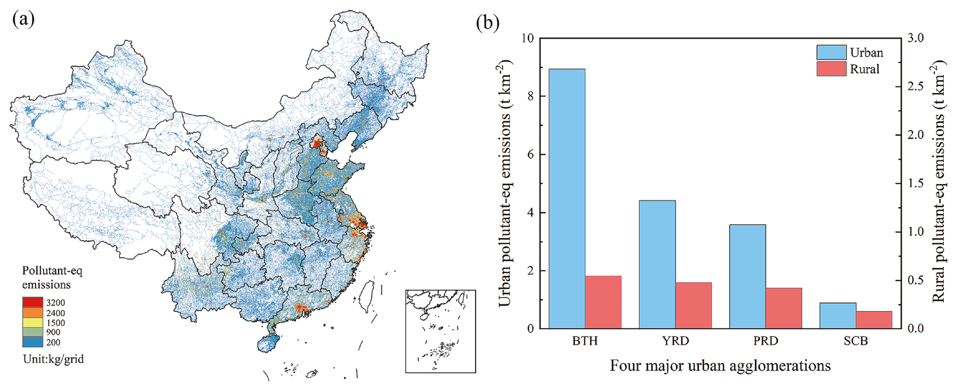
Figure 4 Geospatial distribution of passenger vehicle emissions and the disparities between urban and rural areas: (a) total pollution-eq emissions (TPEs) at 0.01° × 0.01° resolution and (b) urban-rural differences in vehicle emission densities in four major urban agglomerations (BTH: the Beijing-Tianjin-Hebei region; YRD: the Yangtze River Delta region; PRD: the Pearl River Delta region; SCB: the Sichuan Basin) in 2019.

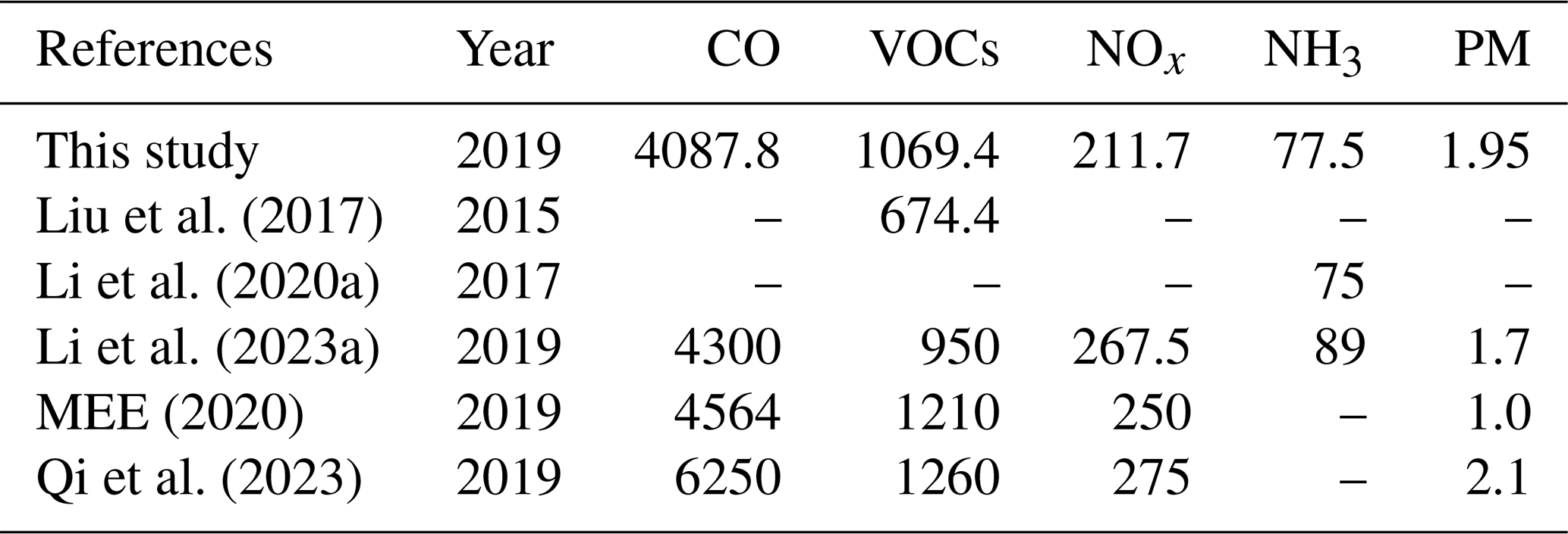
This study conducted a comparative analysis of the results from different studies to verify the accuracy of the emission inventory. Compared with previous research results, this research considered the impact of vehicle driving speed on emissions and the differences in emissions between holiday, workday, and weekend, and its estimated emissions in this study fell within the ranges of other estimation results (Table 1).

Table 1 Comparison and validation with previous studies. (Unit: kt).

3.3 Temporal variation of passenger vehicle emissions

3.3.1 Seasonal and daily variation

Analysis of passenger vehicle emissions revealed distinct seasonal patterns across different regions (Fig. 5). Specifically, the PRD experienced higher emissions in summer, while the YRD, BTH, and SCB regions had higher emissions in winter (Fig. 5c) (Shao et al., 2009; Jiang et al., 2020; Sun et al., 2022). This high winter emission pattern was primarily attributed to adverse weather conditions, which induced prolonged vehicle idling, and reduced driving speeds (Lu et al., 2019). Moreover, vehicles often needed to turn on additional heating equipment, which increased engine load and consequently affected emissions (Abediasl et al., 2023). Notably, Guangdong recorded the highest emissions (Fig. 5a), due to its subtropical climate with approximately 80 % relative humidity (Liu et al., 2020) and had a high volume of traffic (Yang et al., 2022; Krotkov et al., 2016).

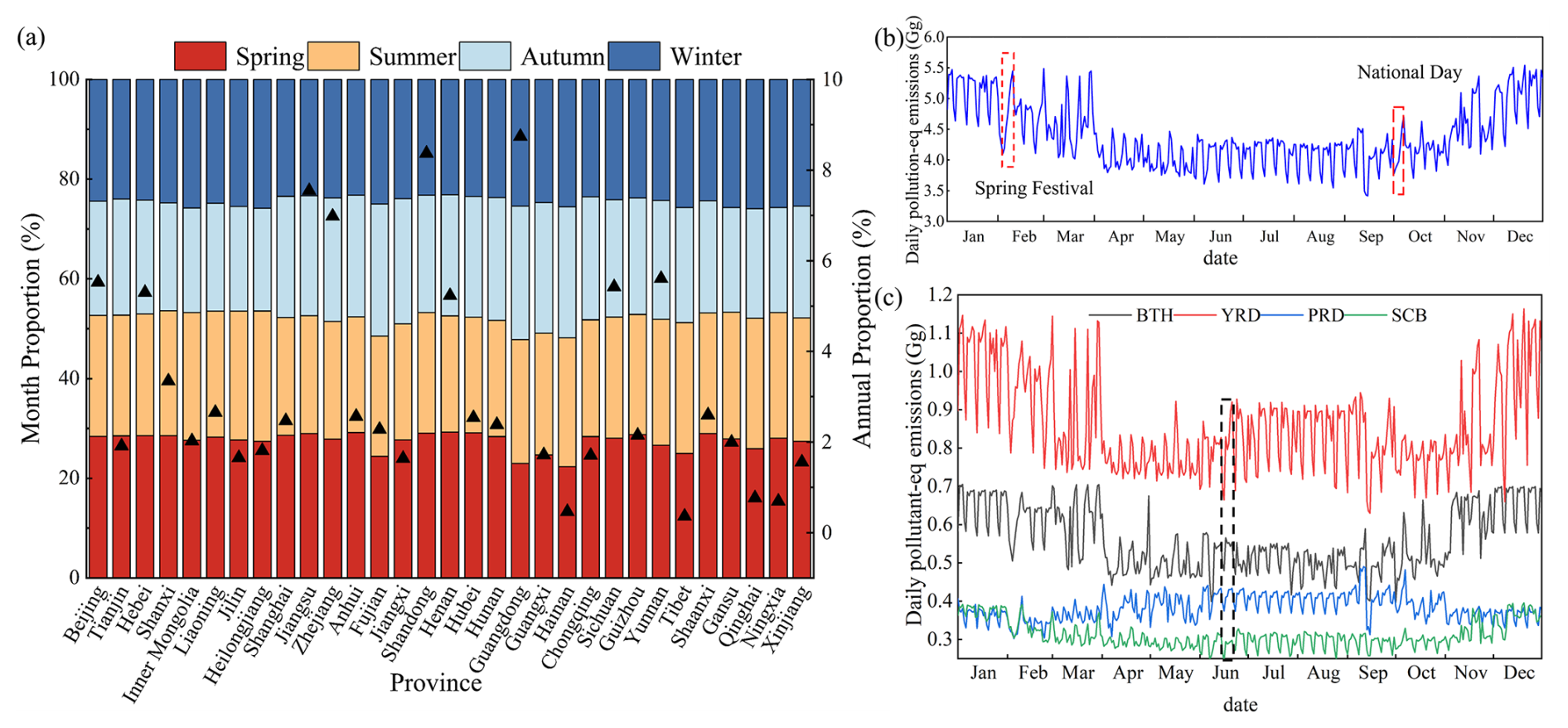
Figure 5 Seasonal and daily scale variations in pollutant emissions: (a) TPEs by province in different months; (b) Daily changes in TPEs across the country and (c) in four major urban agglomerations (BTH, YRD, PRD, SCB).

This study considered the impact of workday, weekend, and holiday on daily emissions. During the Spring Festival and National Day, people opted for public transportation for long-distance travel or returning home at the holiday's onset, resulting in the lowest passenger vehicle emissions on the first day, gradually increasing in the following days (Fig. 5b) (Zhang and Gao, 2023). Passenger vehicle emissions normally exhibited a notable weekend effect, with reduced levels on weekend relative to workday (Fig. S5), and daily average pollutant emissions on holiday were 0.92 times those of workday (Wu et al., 2022; Tong et al., 2020). Specifically at daily emissions, for example, from 17 to 22 June, the BTH, YRD, PRD, and SCB regions exhibited notable differences in emission variations. The YRD and PRD regions experienced emission peaks on Friday, while the BTH reached its highest emission level on Monday, corroborating the findings of Wu et al. (2022) and Zheng et al. (2009).

3.3.2 Hourly variation

The hourly average TPEs varied among workday, weekend, and holiday (Fig. 6a). Peak emission periods were mainly concentrated between 08:00 and 09:00 in the morning and between 16:00 and 17:00 in the afternoon, similar to the daily variation trend of traffic volume (Yang et al., 2019; Shang et al., 2024). During the morning peak, hourly average emissions on workday exceeded those on weekend and holiday by 8 % and 5 %, respectively, increasing to 12 % and 18 % during the evening peak. This expanding difference was attributed to the more diverse types of nighttime travel activities, which included both work trips and daily consumption trips such as dining and shopping. This led to higher vehicle density and prolonged traffic congestion, thereby substantially increasing emission intensity (Azari et al., 2025; Choudhary and Gokhale, 2016). As most private and commercial activities occurred during daylight hours, daytime emissions on workday, weekend, and holiday constituted 85.2 %, 84 %, and 83.1 % of the total daily emissions, respectively.

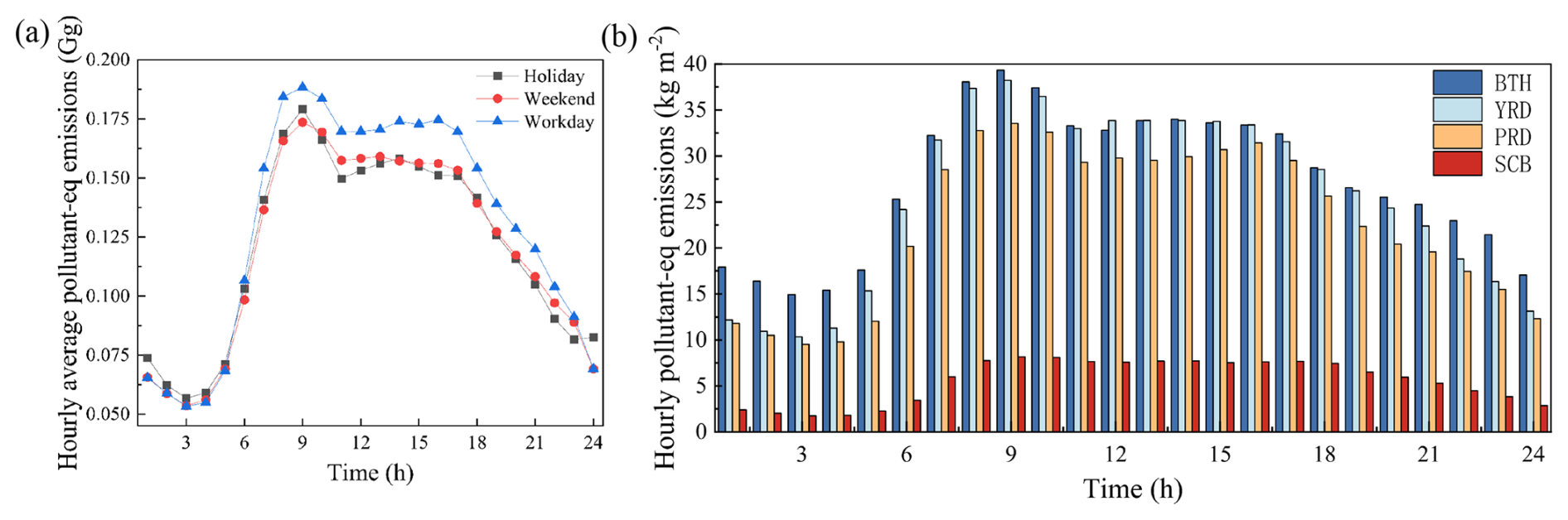
Figure 6 Hourly emission changes for three-day types and regions: (a) hourly total pollutant emission characteristics for weekend, workday and holiday and (b) in four major urban agglomerations (BTH, YRD, PRD, SCB).

A distinct variation in the trend of hourly average TPE density is observed across different regions (Fig. 6b). The BTH region was highest, followed by the YRD, PRD, and SCB regions. This trend might be related to factors such as traffic conditions, population density, and meteorological conditions in each region (Xie et al., 2019; Yang et al., 2025). The data revealed that the daily average emission densities in the BTH and the YRD were 4.9 times and 4.6 times that of the SCB, respectively. Especially during the peak period at 08:00 in the morning, the hourly average emission densities ratios reached as high as 5.4 times and 5.3 times (Fig. 6b). This significant emission difference emphasized the necessity of prioritizing traffic management measures in the BTH region.

3.4 Comparison of passenger vehicle emissions with conventional algorithms

To improve estimation accuracy, this study obtained gridded speed-corrected emission results based on real-time vehicle driving data and compared them with passenger vehicle emission data obtained using traditional methods.

The improved methodology reflected a more accurate and detailed characterization of passenger vehicle emissions, which were primarily concentrated in urban centers, with emission intensity gradually decreasing from the city center outwards (Jing et al., 2016). Spatially, the improved method avoided the limitation of using fixed speeds in traditional approaches. It can accurately identify higher emissions on crowded urban roads caused by frequent acceleration and deceleration, and properly show lower emissions on outside roads (Fig. 7a) (Zhang et al., 2023; Wen et al., 2020; Choudhary and Gokhale, 2016). Overall, the estimation using the traditional method underestimated the total emissions by 31.5 %, with Sichuan, Beijing, Shanghai, and Guangdong being underestimated by 43.1 %, 38.4 %, 29.6 %, and 17.4 %, respectively. In Tibet, the average vehicle speed stabilized at around 42.5 km h⁻¹, and the SCC analysis revealed a speed correction factor 2.09 times that of the traditional speed correction factor (SCF), leading to the most serious underestimation in this region (Fig. 7b) (Sun et al., 2020).

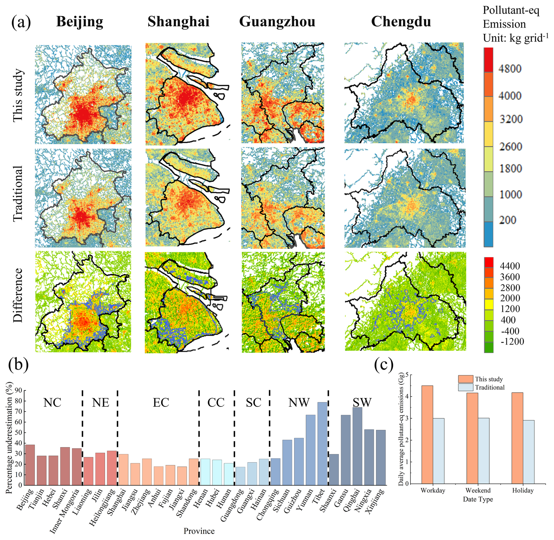
Figure 7 Comparison of this study with traditional algorithms: (a) Beijing, Shanghai, Guangzhou to compare it with the results of the present study (Difference = This Study ­ Traditional); (b) Comparison of daily average results across (c) four seasons and (d) three date type; The percentage of underestimation for each province calculated with the traditional method. The purple boundary in (a) is the Urban Growth Boundary (UGB).

The traditional method exhibited a significant underestimation of passenger vehicle emissions across distinct seasons and day types (Fig. 7c). From a seasonal perspective, this method underestimated the average daily passenger vehicle emissions by 31.6 %, 31.0 %, 32.7 % and 31.8 % in spring, summer, autumn and winter, respectively, with a relatively small overall fluctuation range. In contrast, the discrepancy in underestimation across different day types was more pronounced, and the method's underestimation of passenger vehicle emissions on weekends (33.4 %) was significantly higher than that on weekdays (27.7 %). The formation of this characteristic difference was not only associated with refined vehicle speed correction, but also stemmed from the quantitative analysis of vehicle activity levels across different day types based on congestion indices in this study.

3.5 Model validation

The simulation results of the inventories reflected the temporal variation of pollutant concentrations well. The improved inventory were more consistent with the observed data from the perspective of hourly change (PM_2.5: R²=0.850, NMB = −27.4 %; O₃: R²=0.771, NMB = −32.5 %) (Figs. 8 and S8). The bias may be caused by the underestimation of the input anthropogenic emission inventory, and it falls within an acceptable and reasonable range verified by comparison with other literature (Ma et al., 2018; Wang et al., 2020; Georgiou et al., 2022). This result indicated that the accuracy of the emission inventory refined through detailed vehicle speed correction was superior to that constructed by traditional algorithms.

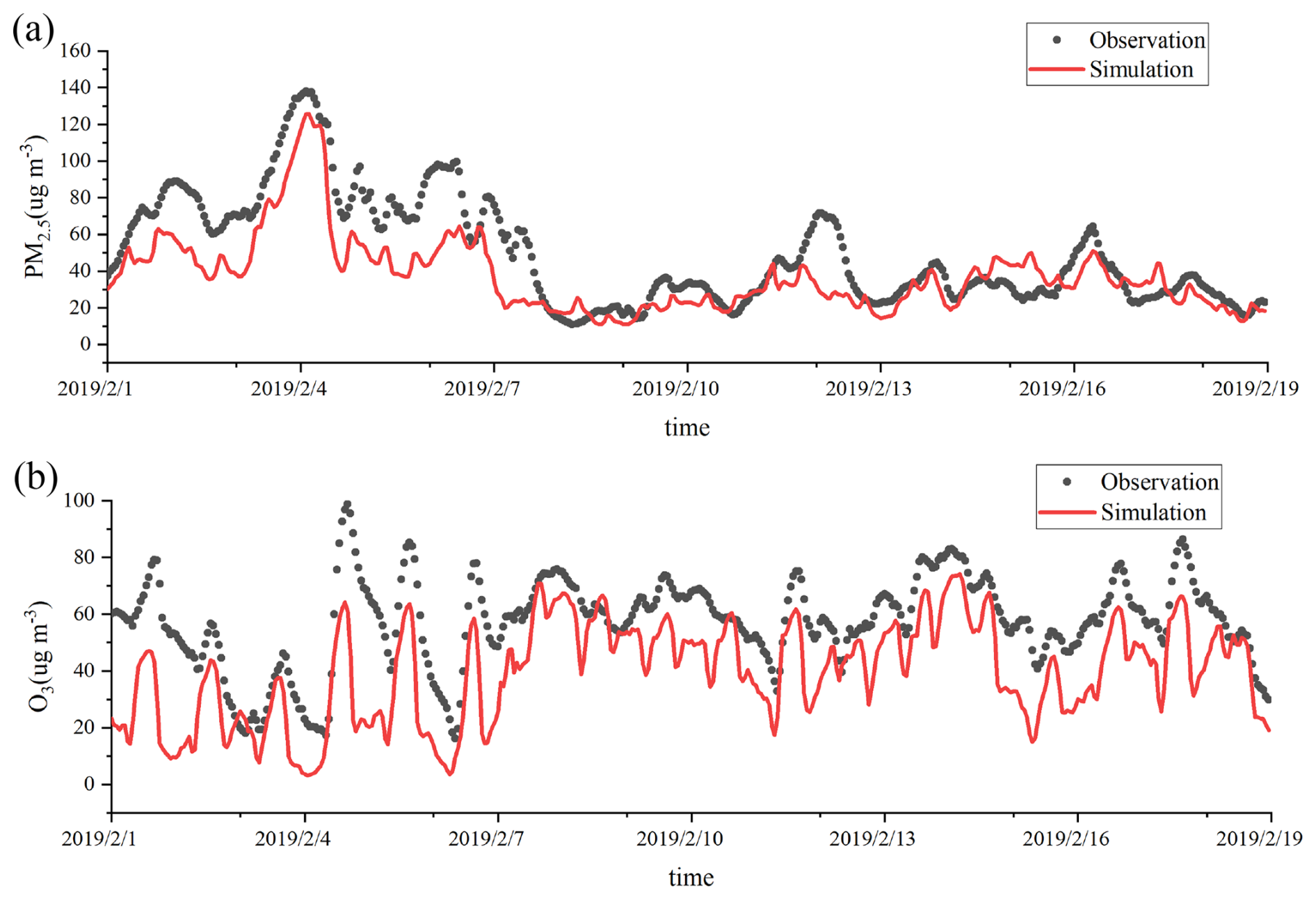
Figure 8 Comparison of temporal variations between simulated results from the improved inventory and observed data. (a) PM_2.5; (b) O₃.

The inventory optimization effect was relatively notable in heavily polluted traffic-intensive areas (Fig. S4b), with an overall 0.36 % improvement in NMB (PM_2.5) and 0.02 improvement in R² (O₃). This effect is attributable to the complex characteristics of speed fluctuations in these areas. Specifically, the NMB of PM_2.5 at the Administrative Center Monitoring Station and Putuo Monitoring Station increased by 0.7 % and 0.45 %, respectively. Meanwhile, the R² of O₃ at the Pudong Chuansha Monitoring Station and Xinghu Garden Monitoring Station rose by 0.05 and 0.04, respectively (Fig. S9). However, this study merely achieved a slight improvement, which may be attributed to the small proportion of emissions from passenger vehicles (e.g., approximately 3.2 % for CO, 4.7 % for VOC, and 1.2 % for NO_x) (Li et al., 2023a). The performance of its simulations would be significantly enhanced when the accuracy of vehicle speed correction for the entire traffic source could be further improved.

4 Conclusions

With the rapid growth of the global automobile industry, the proliferation of passenger vehicles has exacerbated the air pollution problem. Current research lacks a nationwide hourly-scale emissions study for passenger vehicles. Therefore, this study introduces an innovative approach by utilizing big data of ride-hailing services and traffic flow models to obtain nationwide hourly gridded speed and traffic volume, which facilitated the derivation of refined speed correction factors based on actual nationwide driving behavior at both spatial and temporal scales, enabling the construction of a high-resolution (0.01° × 0.01°; 1 h) emission inventory for passenger vehicle atmospheric pollutants in China. Our emission inventory revealed that passenger vehicles in China emitted approximately 4087.8, 1069.4, 211.7, 1.9, and 77.5 kt of CO, VOCs, NO_x, PM, and NH₃, respectively, in 2019.

This research showed significant spatial heterogeneity in passenger vehicle emissions in China. Despite occupying merely 0.8 % of the national territory, urban areas generated 35.3 % of the country's total vehicle emissions. High-pollution areas were predominantly concentrated in four major urban agglomerations (BTH, YRD, PRD, SCB), which contributed significantly to the total emissions at 48.54 %, due to high local traffic volumes and relatively low vehicle speeds. Emission density analysis revealed a hierarchical pattern among urban agglomerations, with the BTH region exhibiting the highest density, followed by the YRD, PRD, and SCB regions. And the urban emission density of vehicles within four urban agglomerations was significantly higher compared to rural areas.

Passenger vehicle emissions also exhibit multiscale temporal variations. Higher emissions observed in winter due to weather and driving conditions. In addition, vehicle emissions normally exhibited a notable weekend effect, with reduced levels on weekend relative to workday, and daily average pollutant emissions on holiday were 0.92 times those of workday. There are also differences in the hourly average pollutant emissions across the above three-day types. During the morning peak, hourly average emissions on workday exceeded those on weekend and holiday by 8 % and 5 %, respectively, increasing to 12 % and 18 % during the evening peak. Compared with traditional algorithms, this study could more accurately identify the actual emission status of urban roads, reducing the deviation in emission estimation. Current traditional methodology might underestimate by 31.5 %, which is more serious in areas with very little speed variation. The simulated results for PM_2.5 and O₃ in this study inventory exhibited good performance.

Our study has limitations in the simulation: Instead of the MEIC anthropogenic emission inventory commonly used in WRF-Chem simulations, we adopted the ABaCAS database for both traffic and non-traffic sources. This is because MEIC does not provide the passenger vehicle emission ratio, which is essential for our accurate estimation of passenger vehicle emission contributions. However, compared with MEIC, ABaCAS underestimates NO_x and VOCs by approximately 20 %, which affects the simulation results to some extent. Previous studies also have reported that the uncertainty ranges of PM_2.5, VOCs and NO_x emissions estimated by ABaCAS are [−58 %, 60 %], [−54 %, 102 %] and [−29 %, 32 %], respectively (Li et al., 2023a). In addition, this may also be related to the insufficient spatial representativeness of national environmental monitoring data during actual acquisition and the influence of local pollution sources around monitoring sites, which slightly affect the validation results (Ding et al., 2024; Zhao et al., 2025; Wu et al., 2018). For these reasons, the simulation results based on ABaCAS database show weak correlation with the temporal variation trend of observed values and strong discrepancies.

At present, this study focuses on passenger vehicles; to improve its accuracy and applicability, future research will be further extended to freight trucks, industrial vehicles, agricultural vehicles, and the entire transportation sector. The speed-emission coupling method verified in this study can not only be extended to such transportation sub-sectors as freight trucks and urban public transport. This improves the accuracy of emission quantification, distinguishes the emission contributions of different vehicle types, and helps to clarify the impacts of anthropogenic nitrogen inputs on the nitrogen cycle (Shen et al., 2026). Meanwhile, the method can also provide revised schemes for aviation and water transportation with different power structures, supporting the establishment of refined emission inventories. In the future, with the continuous increase in the proportion of China V and China VI vehicles, as well as the rising penetration rate of electric vehicles (EVs) (China's stock of electric vehicles reached 31.4 million by 2024, a year-on-year increase of 53.84 %) (MEE, 2025; Liang et al., 2019; Wang et al., 2026), coupled with the implementation of policies for the elimination and renewal of old vehicles, the overall “speed-emission” relationship in the passenger vehicle sector will be gradually weakened (Liu et al., 2024; Zhu et al., 2022). These above-mentioned measures coordinate the upgrading of emission standards with the transformation of the energy structure, providing an important reference for other countries to balance environmental governance, energy security and transportation development. Additionally, a more comprehensive big data will be obtained to provide support for the quality of emission inventories. Overall, the analytical framework developed in this study accurately quantifies emissions of key atmospheric pollutants from China's passenger vehicle sector. The findings provide an important scientific basis for intelligent transportation and the formulation of more refined control policies and offer a methodological reference for precise emission management in the transportation sector through its high-resolution data approach.