Multi-machine-learning approaches to modeling small-scale source attribution of ozone formation

Accurate source apportionment of ozone (O₃) precursors is crucial for implementing scientific O₃ control strategies. While traditional approaches rely on complex calculations of volatile organic compounds (VOCs) and meteorological parameters, their applicability in real-time scenarios remains limited. Taking the Shanghai chemical industrial park as an example, we propose a novel two-step machine learning (ML) approach that integrates positive matrix factorization (PMF) with other ML methods to systematically quantify the spatiotemporal impacts of VOCs on O₃ formation. Analysis of high-frequency data from 12 VOC monitoring stations (2021–2023) using six ML models revealed XGBoost as the optimal predictor (R²=0.644) for local VOC emissions. By combining SHapley Additive exPlanations (SHAP) with ML modeling, we precisely evaluated VOC–O₃ relationships and located emission sources. Results identified solvent use (SU) and fuel evaporation (FE) as primary O₃ formation contributors, followed by combustion sources (CS) and vehicle emissions (VE). PMF analysis further distinguished six VOC sources: petrochemical processes (PP), FE, CS, SU, polymer fabrication (PF) and VE. Temporal analysis revealed seasonal variations, with CS and FE dominant in spring/summer, while PF prevailed in autumn. This innovative framework demonstrates exceptional capability for rapid source identification and precise contribution quantification, establishing a new paradigm for high-resolution O₃ source apportionment.

1 Introduction

Ozone (O₃) pollution has become a significant environmental issue, posing serious threats to human health and ecosystems worldwide (Long et al., 2023; Sharma et al., 2023; Masui et al., 2023; Sharma et al., 2024). In particular, industrial parks, which are characterized by high levels of anthropogenic emissions, serve as critical hotspots for the formation of ground-level O₃ due to the abundance of precursor pollutants such as volatile organic compounds (VOCs) and nitrogen oxides (NO_x) (Pinthong et al., 2022; Kim et al., 2023; He et al., 2024). From the current point of view, the pollution characteristics and sources of VOCs in industrial parks are relatively more complex (Cao et al., 2024). Understanding the contribution of VOCs to O₃ formation is essential for developing effective mitigation strategies aimed at reducing air pollution and improving air quality.

At present, VOC source identification technology mainly includes source emission inventories (Lu et al., 2025), chemical transport models (CTMs) (Choi et al., 2020; Wang et al., 2023) and receptor models (Wu et al., 2023). Traditionally, the quantification of VOC contributions to O₃ formation has relied heavily on CTMs, which require detailed knowledge of atmospheric chemistry and complex computational resources (Li et al., 2014). However, these models often suffer from uncertainties related to emission inventories and chemical mechanisms (Sharma et al., 2017; Baklanov and Korsholm, 2008). In addition, the detailed input data and computing power requirements of CTMs leave some areas for improvement (Nelson et al., 2023). The receptor model has the advantages of fewer hardware requirements, higher precision and easy configuration, among which the positive matrix factorization (PMF) model has been widely used to identify VOC emission sources (Tan et al., 2021; Yang et al., 2023). However, it should be emphasized that PMF and CTMs are methodologically distinct: CTMs simulate physico-chemical processes driven by emission inventories and meteorology, enabling dynamic regional-scale predictions, whereas PMF statistically decomposes sources based on covariance in observed species concentrations. While PMF demonstrates strong performance in settings with spatially dense monitoring, its accuracy is inherently constrained by input data representativeness and chemical stability of source profiles. Consequently, PMF is best positioned as a complementary tool for CTMs in integrated assessment frameworks. PMF models are typically combined with the O₃ formation potential (OFP) calculated by the maximum incremental reactivity (MIR) value of VOC species (Carter, 2010) to assess the relationship between VOCs and O₃ concentrations (Xiao et al., 2024). As the key parameter MIR value used in this method is usually calculated based on 39 cities in the United States where O₃ exceeds the standard, whether the MIR value can fully reflect the contribution of VOCs to O₃ under complex atmospheric pollution conditions in China is controversial (Zhang et al., 2021). Furthermore, conventional methods like PMF, while effective for source categorization, face critical limitations: they cannot differentiate rapid O₃ formation via photostationary state perturbations (e.g., alkene depletion) from slower HO_x-mediated pathways (e.g., alkane oxidation) (Sillman, 1999). This mechanistic gap introduces spatiotemporal biases when quantifying source contributions in chemically complex environments like coastal petrochemical zones. To address these challenges, our study integrates interpretable machine learning (ML) with PMF, explicitly resolving fast vs. slow O₃ production pathways while leveraging the study area's unique spatial and industrial characteristics.

In recent years, more ML techniques have emerged as powerful tools for analyzing complex datasets and predicting environmental phenomena (Salcedo-Sanz et al., 2024; Essamlali et al., 2024). However, the “black box” nature of ML models makes their results difficult to interpret and generalize to real scenarios (Guidotti et al., 2018). Recently, the SHapley Additive Interpretation (SHAP) algorithm has been applied to solve these problems (Louhichi et al., 2023; Li et al., 2024; Lundberg and Lee, 2017). Novel ML approaches can provide robust predictions with less reliance on mechanistic details, making them attractive alternatives or complementary methods to traditional ML models. To address these gaps, we integrate PMF with other advanced ML methods to develop a two-step ML framework. This approach not only enhances the efficiency and accuracy of data analysis but also addresses the limitations of traditional PMF methods under complex environmental conditions, providing a more robust solution for pollution source identification and contribution analysis.

In the past, researchers have used different ML models to study the transformation mechanism of O₃ and its precursors (Cheng et al., 2024; Kuo and Fu, 2023). More recently, ML-coupled receptor models have been used to better identify and quantify the drivers of pollutants. For example, Cheng et al. (2023) assessed the impact of emission sources on O₃ formation by combining PMF with four ML models. Chen et al. (2024) used a PMF model combined with the Category Boosting (CatBoost) model and the Shapley additive interpretation algorithm to quantify the influence of pollution sources and meteorological factors on VOCs. Ning et al. (2024) constructed a cross-stacked ensemble learning model (CSEM) to predict O₃ concentrations under different NO_x and VOC emission reduction scenarios.

Our study focuses on a coastal petrochemical industrial zone in Shanghai, where proximity to the ocean and dense aggregation of ethylene crackers and aromatics plants create a unique microenvironment. High humidity and solar irradiance amplify atmospheric oxidative capacity (Zhang et al., 2021), while emissions of short-lived unsaturated VOCs (e.g., propylene, 1,3-butadiene) drive rapid O₃ formation via alkene-NO_x reactions within <50 km under sea–land breezes (3–5 m s⁻¹) (Zhang et al., 2025; Zhao et al., 2022; Wang et al., 2018). Additionally, our study pioneers high-resolution source attribution (1 km × 1 km) in a coastal petrochemical cluster in Shanghai, a methodology particularly suited to resolve localized ozone production under elevated regional backgrounds (>80 ppb). By leveraging the unique microenvironment of dense ethylene crackers and aromatics plants adjacent to the ocean, we isolate rapid photochemical processes driven by short-lived, highly reactive VOCs (e.g., propylene, 1,3-butadiene; atmospheric lifetime <6 h) that dominate O₃ formation within <50 km.

Considering the advantages of the diverse types and complex sources of VOCs in chemical industrial parks, this characteristic enhances model robustness and improves the model's feature extraction capabilities. This study selected a chemical industrial park in Shanghai as an ideal case for model training. In this study, we present a novel small-scale approach that integrates multiple ML models to quantify the impact of VOCs on O₃ formation with unprecedented spatial resolution. Our methodology harnesses the analytical power of ML algorithms to process high-frequency data from 12 strategically positioned VOC boundary monitoring stations, enabling rapid and accurate source identification at a fine-grained spatial scale previously unattainable through conventional methods. The analytical framework consists of three sophisticated components: first, we conduct a systematic evaluation of diverse ML algorithms to identify the optimal model configuration, ensuring robust predictive performance at the local scale. Subsequently, we leverage the interpretable ML technique SHAP to quantitatively assess VOC–O₃ relationships and precisely pinpoint emission sources with high spatial accuracy. Finally, we develop an innovative hybrid approach that combines PMF for source apportionment with ML-SHAP analysis to achieve rapid and precise identification of key pollution sources contributing to O₃ formation at the facility level. This advanced methodological framework demonstrates significant advantages in both efficiency and spatial precision: it enables swift identification of specific emission sources while maintaining high accuracy in quantifying their individual contributions to O₃ formation. The approach transcends traditional analytical limitations by offering a powerful tool for high-resolution source traceability, thereby providing crucial support for implementing targeted and effective O₃ control strategies at the facility or district level. Moreover, this novel integration of multiple analytical techniques establishes a new paradigm for addressing complex air quality challenges through sophisticated data-driven approaches that bridge the gap between regional-scale analysis and facility-level source identification.

2 Material and methods

2.1 Study area and data details

The Jinshan District is located in the southwestern part of Shanghai, along the northern shore of Hangzhou Bay (HZB) at geographical coordinates 30°40^′–30°58^′ N and 121–121°25^′ E, covering a total land area of 586.05 km² (Fig. 1). It is recognized as an important resource-based city. The Jinshan Industrial Zone, situated in the southeastern part of Jinshan District, serves as a fine chemical industrial park. Within and surrounding the industrial zone, 12 monitoring stations have been established to assess the environmental air quality in the area (as detailed in Table S1 in the Supplement). The distribution of these monitoring stations is illustrated in Fig. 1. Hourly O₃ concentration data utilized in this study were obtained from the Atmospheric Environmental Monitoring Routine Data Management System of the Shanghai Environmental Monitoring Station (https://github.com/bobooob/Multi-machine-learning-approaches, last access: 29 April 2026). The concentration data for VOCs were sourced from the 12 monitoring stations and can be accessed through the Intelligent Analysis System for VOC Emissions and Pollution Source Tracing in Key Industrial Parks of Shanghai (https://github.com/bobooob/Multi-machine-learning-approaches, last access: 29 April 2026). The dataset covers a collection period from 1 January 2021 to 31 December 2023, with measurements recorded on an hourly basis.

Two types of VOC monitoring instruments were deployed at the boundary observation stations. The first type utilized gas chromatography–flame ionization detector (GC-FID) technology, featuring low-carbon (C₂–C₅) and high-carbon (C₆–C₁₂) analyzers (Synspec GC955-615/815, Juguang Technology Co., Ltd.; A11000/A21022, Chromatotec Inc., France; Spectra SYS GC3000-315L/H, Pu Yu Technology Development Co., Ltd.) and enabling automatic hourly measurements of 89 VOC species. The second type employed a combined GC-FID and mass spectrometry (GC-FID/MS) approach, which included FID detection for C₂–C₅ aromatic hydrocarbons and mass spectrometry detection for other compounds. The instrument operated by sampling at 30 L min⁻¹ for the initial 10 min each hour, utilizing a cryogenic cold trap for sample preservation before separation and detection on specific chromatographic columns. Quality assurance and quality control (QA/QC) protocols adhered to the “Technical Specifications for Operation and Quality Control of Continuous Automatic Monitoring Systems for Gaseous Pollutants in Ambient Air” (HJ 818-2018), issued by China's Ministry of Ecology and Environment. Daily checks ensured data completeness and chromatogram integrity, with any detected abnormalities prompting immediate on-site maintenance. Routine data audits involved the removal of abnormal data, while measurement accuracy was verified biweekly, with calibration curves, method detection limits (MDLs) and instrument precision assessed quarterly. Standard gas accuracy checks showed relative errors below 20 %, and in blank tests, absolute errors were less than 0.3 ppbv. Calibration curves were established using five standard gases (1, 5, 10, 15 and 20 ppbv), yielding correlation coefficients greater than 0.995, and MDLs for PAMS and TO-14 species were maintained at or below 0.3 and 0.5 ppbv, respectively. Throughout the study period, a total of 26 280 sets of VOC data were collected, resulting in the identification of 36 distinct VOC species, comprising 12 alkanes, 7 alkenes, 11 aromatics and 6 halogenated hydrocarbons after data screening.

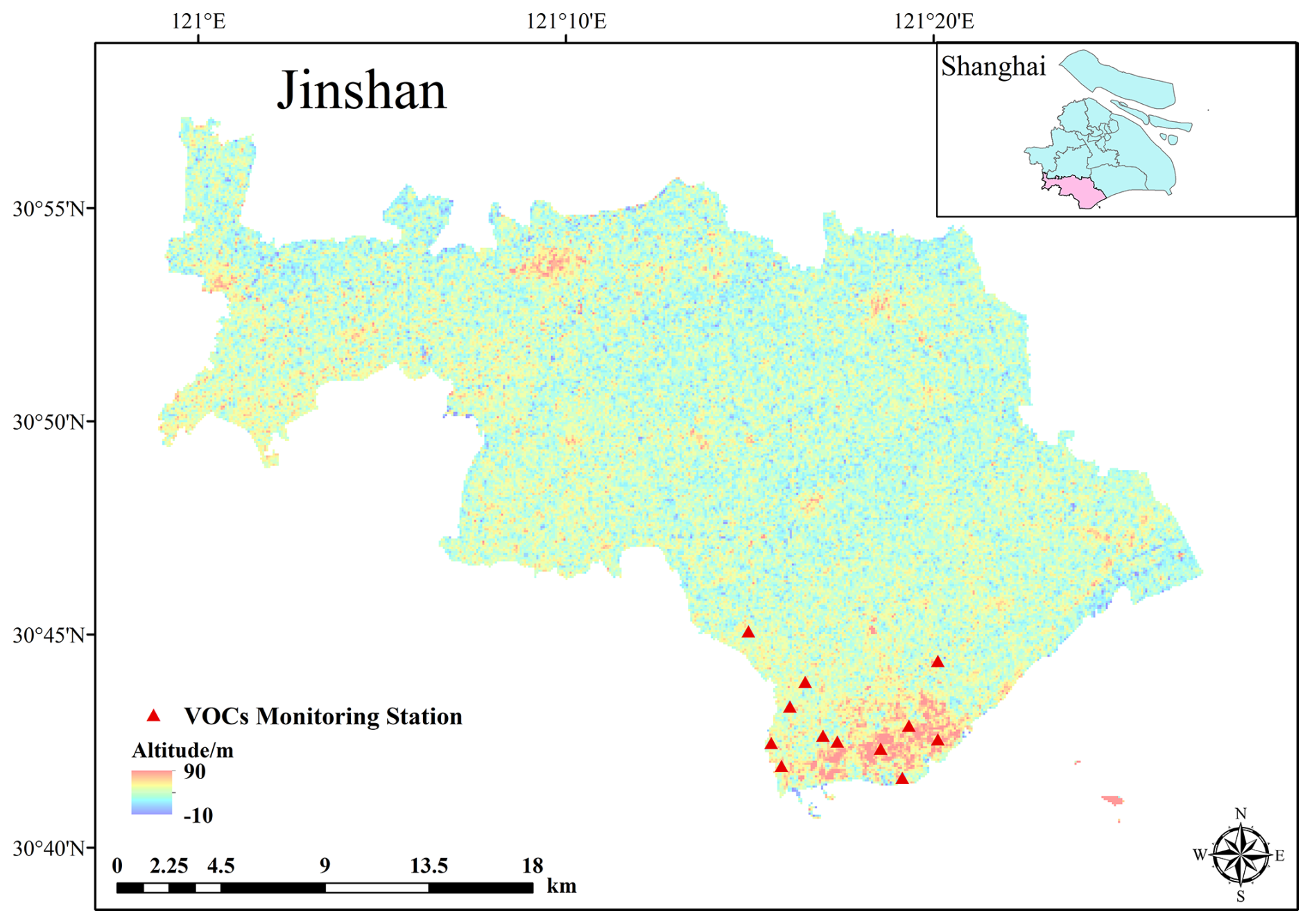
Figure 1 Study area and sampling sites. The triangles indicate the 12 sites utilized for the evaluation of the model.

2.2 Positive matrix factorization model (PMF)

The PMF 5.0 software, developed by the United States Environmental Protection Agency (EPA), is widely utilized to assess and quantify the contributions from various sources to samples based on their chemical composition or unique fingerprints. Initially introduced by Paatero (1997) at the University of Helsinki, this model decomposes the sample matrix (which is non-negative) into two distinct matrices: the source contribution matrix (g) and the source component spectral matrix (f). The least-squares method is subsequently employed to estimate the contribution rates and identify major pollution sources, with the objective of minimizing the discrepancy between the calculated Q value and the theoretical Q value. The formulation of the PMF model is represented by Eq. (1):

$$\begin{array}{}\text{(1)}& e_{ij}=x_{ij}-\sum _{k=\mathrm{1}}^p{g}_{ik}{f}_{kj},\end{array}$$

where X_ij represents the concentration of jth species in the ith sample, g_ik represents the concentration of kth source in the ith sample, f_kj represents the mass percentage of jth species in the kth sample, and e_ij represents the residue factor for jth species in the ith sample.

In the PMF model, factor contributions and source fingerprint spectra are derived by minimizing the objective function (Q), as described in Eq. (2):

$$\begin{array}{}\text{(2)}& Q=\sum _{i=\mathrm{1}}^n\sum _{j=\mathrm{1}}^m\left(\right(x_{ij}-\sum _{k=\mathrm{1}}^p{g}_{ik}{f}_{kj})/u_{ij}{)}^{\mathrm{2}}.\end{array}$$

The uncertainty (u_ij) of the jth species in the ith sample is calculated by considering the minimum detection limit (MDL) and error scores of each species.

Crucially, PMF resolves source-specific contributions to VOC mass concentrations (g matrix), not directly to ozone formation. To attribute ozone impacts, we integrate the PMF-derived g matrix as inputs to machine learning models.

2.3 Machine learning models

To explore data characteristics and select the optimal ML model, we utilized data from the Jinshan Industrial Zone covering the period from January 2021 to December 2023 for training and evaluating ML models. In this study, hourly data of O₃ and total volatile organic compound (TVOC) concentrations from 12 monitoring stations were input into the ML models. The dataset was partitioned into training (70 %) and testing (30 %) subsets using chronological splitting to preserve temporal integrity. Model robustness was further validated via 10-fold cross-validation on the training set. Subsequently, the ML models were integrated with the SHAP (SHapley Additive exPlanations) (Sect. S1.2 for model details) framework to obtain SHAP values for the 12 stations, quantifying their contributions to O₃ formation. SHAP values quantify the relative influence of input features (e.g., site-specific TVOC concentrations) on ML-predicted O₃ levels – not absolute physicochemical contributions to ozone formation. Higher absolute SHAP magnitudes indicate stronger feature importance in the model's decision-making, enabling spatial prioritization of emission hotspots. The stations contributing the most to O₃ were identified, and the source of characteristic VOC data was recognized using the PMF model. The emission factors derived from the PMF analysis, along with hourly O₃ concentration data, were then input into the ML models for SHAP analysis. Finally, the optimal ML model and the most severe pollution sources were identified. The source contribution matrix (g matrix) derived from PMF analysis, representing the hourly contribution rates (%) of the six resolved sources, served as input features alongside concurrent O₃ concentration data for training the machine learning models. This approach transformed source apportionment results into predictive variables for O₃ formation modeling. Subsequently, the SHAP algorithm was applied to quantify the contribution of each PMF-resolved source to O₃ predictions generated by the optimized ML model, enabling high-resolution attribution of emission sources to ozone formation dynamics.

In this study, we implemented six ML models, including Decision Tree Regression (DTR), Random Forest Regression (RF), Support Vector Regression (SVR), XGBoost Model, CatBoost Model and LightGBM Model (refer to Sect. S1.1 for model details). Compared to complex deep learning architectures (e.g., CNNs, RNNs), these models offer distinct advantages for high-dimensional spatiotemporal datasets: (1) native support for feature importance metrics (e.g., Gini, permutation importance) enables direct interpretation of predictor contributions without post hoc explainers, (2) computational efficiency facilitates rigorous hyperparameter optimization with Bayesian methods and (3) robustness to collinear features common in atmospheric chemistry (Pichler and Hartig, 2023; Kaur et al., 2020). Bayesian optimization (Robin et al., 2021) was then applied to determine optimal hyperparameters across more the 120 000 hourly samples. Detailed implementation procedures of Bayesian optimization, including model-specific hyperparameter spaces, convergence criteria and computational configurations, are comprehensively documented in Sect. S1.3 of the Supplement. Ultimately, through iterative optimization of training configurations (70:30 train–test partitioning, 10-fold cross-validation) and six repetitions of randomized initialization experiments with distinct random seeds (Seed = 42, 87, 124, 256, 512, 1024), we selected the model with the highest R² from the six ML models, along with its corresponding parameter combinations, as the optimal ML model. Additionally, to assess the robustness and stability of the models, we employed mean absolute error (MAE) and root mean squared error (RMSE) as evaluation metrics.

R² is an indicator that measures the overall goodness of fit of a regression model, and its calculation is shown in Eq. (3):

$$\begin{array}{}\text{(3)}& R^{\mathrm{2}}=\mathrm{1}-{\displaystyle \frac{\sum _{i=\mathrm{1}}^n{\left(y_i-{\widehat{y}}_i\right)}^{\mathrm{2}}}{\sum _{i=\mathrm{1}}^n{\left(y_i-\overline{y}\right)}^{\mathrm{2}}}},\end{array}$$

where y_i represents the actual observed values, ${\widehat{y}}_i$ denotes the predicted values, $\overline{y}$ is the mean of the actual observed values, and n indicates the total number of observations.

MAE is the average of the absolute differences between the predicted values and the actual values, as calculated in Eq. (4):

$$\begin{array}{}\text{(4)}& \text{MAE}={\displaystyle \frac{\mathrm{1}}{n}}\sum _{i=\mathrm{1}}^n\left|y_i-{\widehat{y}}_i\right|,\end{array}$$

where y_i is the actual observed value, ${\widehat{y}}_i$ is the predicted value and n is the total number of observations.

RMSE is the square root of the average of the squared differences between the predicted values and the actual values, as shown in Eq. (5):

$$\begin{array}{}\text{(5)}& \text{RMSE}=\sqrt{{\displaystyle \frac{\mathrm{1}}{n}}\sum _{i=\mathrm{1}}^n{\left(y_i-{\widehat{y}}_i\right)}^{\mathrm{2}}},\end{array}$$

where y_i represents the actual observed values, ${\widehat{y}}_i$ denotes the predicted values and n is the total number of observations. This metric provides insight into the model's accuracy by giving a higher weight to larger errors, making it sensitive to outliers.

To ensure data integrity, a thorough check for missing values was conducted on the original observational data prior to its input into the machine learning models. Subsequently, these missing values were imputed using the RF model, and validation was performed using the available observational data. The resulting dataset was then transformed into a supervised learning dataset with time-dependent features. To guarantee the accuracy of the experiments, 70 % of the dataset was consistently used as the training set and 30 % as the test set for each ML model. Hyperparameter tuning was performed utilizing the Bayesian optimization technique. Furthermore, to mitigate the influence of model randomness on the test set results, all ML models underwent 10-fold cross-validation experiments.

In this study, the ML models and the SHAP algorithm were primarily implemented using Python 3.6 and Anaconda 4.5 platforms. The research methodology framework used in this study is shown in Fig. 2.

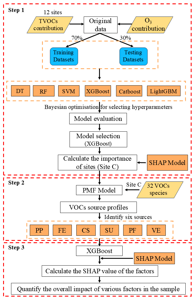
Figure 2 Schematic workflow of the integrated ML–PMF framework for ozone source attribution (see Sect. 2.3 for methodological details).

3 Results and discussions

3.1 Spatiotemporal characterization of ozone and VOC concentrations: a multi-scale analysis for enhanced ML performance

A comprehensive understanding of the spatiotemporal characteristics of the input dataset is fundamental for optimizing machine learning model interpretability and performance. Our analysis of VOC and O₃ concentrations across multiple monitoring sites from 2021 to 2023 reveals distinct patterns that inform our ML-based source attribution approach. The temporal evolution of O₃ concentrations shows a notable progression, with mean values of 64.45, 68.79 and 68.90 µg m⁻³ recorded in 2021, 2022 and 2023, respectively (Fig. 3a). The relatively lower O₃ levels observed in 2021 coincide with the COVID-19 pandemic period, when reduced anthropogenic activities, particularly decreased vehicular traffic and industrial operations, significantly altered urban emission patterns in Shanghai (Lu et al., 2023). A marked reduction in VOC concentrations was observed across all monitoring sites in 2022, primarily attributed to the implementation of stringent emission control measures by local regulatory authorities (Xiao et al., 2024). The seasonal analysis reveals distinctive O₃ formation patterns in the study area (Fig. 3b). O₃ concentrations exhibit a rapid acceleration during spring, reaching maximum levels in May, followed by a notable decline during the summer months (June–August). This pattern differs from typical urban environments, as Shanghai's unique high-pressure meteorological conditions drive peak daytime O₃ levels in late May with unprecedented rates of increase (Chang et al., 2021). Notably, elevated VOC concentrations coincide with the June industrial maintenance period, providing critical temporal markers for our ML-based source attribution.

The diurnal profile analysis (Fig. 3c) reveals sophisticated photochemical patterns that enhance our ML model's temporal resolution. O₃ concentrations follow a characteristic curve, initiating a rapid increase at 08:00 (UTC+8), sustaining growth until reaching peak levels at 15:00, followed by a gradual decline. This pattern aligns with the intensification of photochemical reactions driven by increasing solar radiation. The observed dual-peak pattern in VOC concentrations (06:00–08:00 and 19:00–22:00) corresponds to industrial operational cycles, providing essential precursor availability for daytime O₃ formation. This rich temporal diversity in our dataset significantly enhances the ML model's capability to capture complex source–receptor relationships.

The correlation analysis provides crucial insights for optimizing our ML framework's feature selection and interpretation capabilities (Fig. 3d). The heterogeneous correlations between VOCs and O₃ across monitoring sites reveal complex source–receptor relationships: while most sites exhibit negative correlations, Sites D and K show positive associations. Notably, Sites C ($r=-\mathrm{0.12}$) and L ($r=-\mathrm{0.081}$) demonstrate the strongest negative correlations, marking them as critical locations for detailed feature importance analysis in our ML framework. These diverse correlation patterns enhance our model's ability to capture local-scale emission–concentration relationships, crucial for precise source attribution.

Figure 3 Temporal and spatial dynamics of VOCs and O₃, along with their correlations, as observed at 12 monitoring stations. (a) Mean concentration variations of O₃ and VOCs from 2021 to 2023. (b) Monthly profiles of O₃ and VOC concentrations. (c) Daily profiles of O₃ and VOC concentrations. (d) The correlation matrix between O₃ and VOC measurements at the 12 monitoring sites.

3.2 Comparison of ML models

3.2.1 Model performance evaluation and selection of optimal ML algorithm

The selection and evaluation of appropriate machine learning algorithms are fundamental to ensuring robust and reliable analytical outcomes, particularly when dealing with complex environmental datasets (Liu et al., 2022). In this investigation, we implemented and systematically evaluated six state-of-the-art machine learning algorithms: DT, RF, SVM, XGBoost, CatBoost and LightGBM. These models were rigorously trained and tested using spatially distributed VOC and O₃ monitoring data from multiple sampling sites.

The comparative performance metrics of these models are comprehensively presented in Table 1. Notably, R² values obtained through 10-fold cross-validation demonstrated remarkable consistency with those derived from the independent test dataset. This concordance strongly indicates the robust generalization capabilities of our machine learning framework, suggesting effective pattern recognition within the data while avoiding overfitting issues. Among the evaluated algorithms, the XGBoost model demonstrated superior predictive performance across all assessment metrics. Specifically, it achieved the lowest MAE of 13.828, mean absolute percentage error (MAPE) of 0.445 and RMSE of 11.620, coupled with the highest R² value of 0.637.

Further validation through scatter plot analysis (Fig. S2) revealed that the XGBoost model exhibited significantly smaller deviations between predicted and observed values compared to other algorithms, confirming its enhanced predictive accuracy. Based on these comprehensive evaluation results, the XGBoost model was selected as the optimal algorithm for O₃ concentration prediction. Consequently, the subsequent SHAP analysis was conducted exclusively on the XGBoost model to ensure the highest level of interpretability and reliability of source attribution results.

Table 1 Comparison of six ML models based on different evaluation metrics.

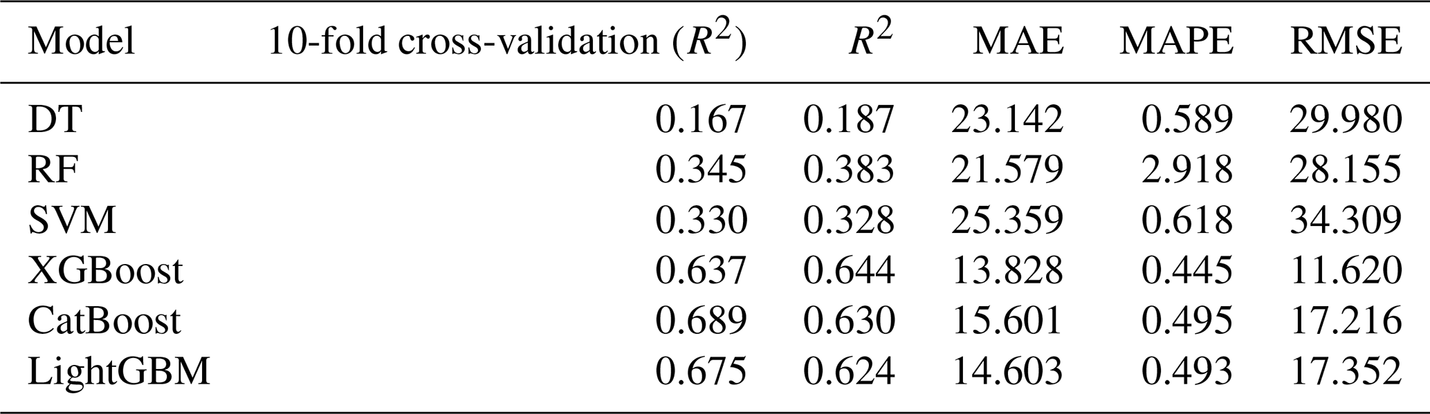
MAE: mean absolute error, MAPE: mean absolute percentage error, RMSE: root mean squared error, DT: decision tree, RF: Random Forest, SVM: Support Vector Machine, XGBoost: Extreme Gradient Boosting, CatBoost: Category Boosting, LightGBM: Light Gradient Boosting Machine

3.2.2 Spatial distribution analysis of TVOC contributions using SHAP interpretation

To quantitatively assess the spatial heterogeneity of TVOC contributions to O₃ formation, we conducted a comprehensive SHAP analysis across all monitoring sites within the established XGBoost regression model (Fig. 4). The analysis revealed distinct patterns of TVOC influence, with Site C demonstrating notably dispersed sample distribution patterns, indicating its predominant influence on O₃ formation dynamics. The analysis identified a significant negative correlation between TVOC concentrations at Site C and model predictions, evidenced by the high-magnitude SHAP values concentrated in the negative region. This SHAP-negative TVOC signal reflects the model's recognition of Site C's unique emission mix, where VOC-rich plumes initially suppress ozone via NO titration under proximate NO_x-rich conditions but subsequently fuel downwind ozone formation as air masses age and transition to VOC-limited chemical regimes. This duality aligns with observational studies in petrochemical clusters, where proximal VOC hotspots exhibit transient O₃ suppression due to localized precursor interactions while driving net regional ozone increases through secondary photochemical pathways (Guo et al., 2022; Ren et al., 2024). Conversely, Site K exhibited a strong positive correlation, characterized by elevated SHAP values consistently distributed in the positive region, corroborating the correlation analysis findings presented in Sect. 3.1.

The pronounced influence of Site C can be attributed to its strategic location within the southeastern sector of the Jinshan Chemical Zone, where it is surrounded by diverse industrial activities. The site's immediate vicinity encompasses plastic manufacturing facilities to the east, a petroleum products transportation port to the south, chemical production facilities to the west and a public transportation hub featuring five gas stations to the north. This complex industrial landscape surrounding Site C facilitates intensive O₃ formation while presenting significant challenges for precise source attribution of TVOC emissions.

To validate the robustness of these findings, we extended the SHAP analysis to encompass five additional ML models (Fig. S3). The results consistently identified Site C as the most influential monitoring location across all model analyses, substantiating its critical role in local O₃ formation processes. This convergence of results across multiple ML platforms reinforces the reliability of our spatial analysis and highlights the importance of Site C in understanding regional O₃ pollution patterns. Importantly, SHAP values here reflect the relative importance of each site's TVOC concentrations to XGBoost-predicted O₃ – not direct source contributions. This approach identifies locations where VOC variations most strongly perturb O₃ predictions (e.g., Site C's dominant role), guiding subsequent PMF-based source apportionment.

In addition, to ensure robustness of feature importance interpretations, we employed three complementary attribution schemes beyond SHAP: (1) SAGE (Shapley Additive Global importance) for global feature relevance; (2) Gini importance for intrinsic tree-based rankings and (3) permutation importance evaluating prediction degradation under feature shuffling. Figure S6 compares normalized importance scores across SHAP, SAGE, Gini and permutation methods for the sites. For Site C, SHAP, SAGE and permutation importance uniformly assign it the highest score (normalized score ≈1.0), confirming its dominance in prediction-sensitivity-based frameworks. In contrast, Gini importance ranks Site C third (normalized score ≈ 0.6). To further quantify the consistency of feature importance rankings across methodologies, we computed pairwise Pearson correlation coefficients between SHAP, SAGE, Gini and permutation importance scores (Fig. S7). The correlation matrix reveals near-perfect agreement between SHAP, SAGE and permutation importance (Pearson r=0.98 for all inter-method pairs), confirming these techniques capture overlapping dimensions of feature relevance tied to global prediction sensitivity. In contrast, Gini importance exhibits weak correlation with the other three schemes (r≤0.12). This divergence arises because Gini importance prioritizes local decision-tree split purity (e.g., maximizing variance reduction at individual nodes), which can overemphasize features with high within-tree variability but low global relevance to ozone photochemistry. Conversely, SHAP, SAGE and permutation – grounded in global prediction sensitivity – robustly identify Site C as the primary driver of O₃ formation, as their concordance (r=0.98) reflects shared sensitivity to chemically meaningful VOC–O₃ interactions. Thus, the methodological triangulation of SHAP, SAGE and permutation – coupled with Gini's demonstrated insensitivity to global photochemical dynamics – unequivocally confirms Site C's preeminent role in regional ozone formation.

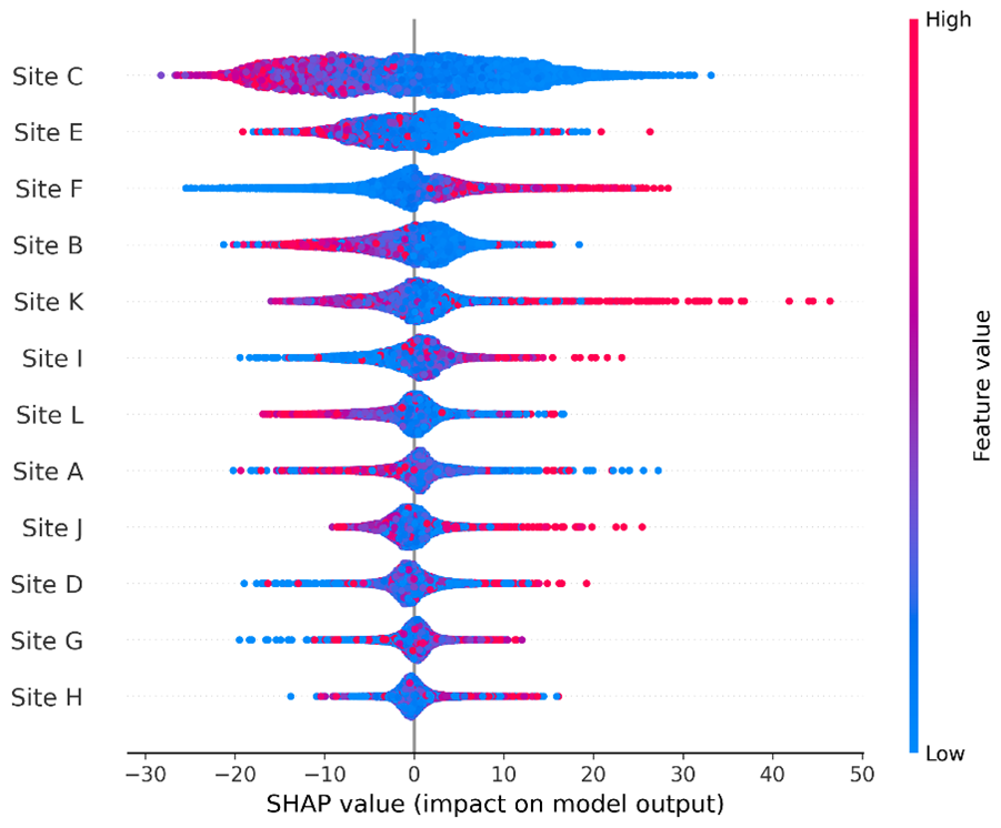
Figure 4 Feature importance of total volatile organic compound (TVOC) drivers obtained by XGBoost model. Blue points indicate negative contributions to the prediction, while red points represent positive contributions.

3.3 Source apportionment and temporal–spatial characterization of VOCs based on the PMF model

3.3.1 Analytical framework and results of the PMF model

Inter-species correlation analysis revealed distinct clustering patterns among VOCs (Fig. S4). Strong positive correlations (r>0.7) were observed among alkane homologues such as ethane (C₂), propane (C₃), n-butane (C₄) and isopentane (C₅) (r=0.71–0.92), indicative of co-emission from fuel evaporation and petrochemical activities (Yang et al., 2024). Strong positive correlations were observed between propylene and 1,3-butadiene (r=0.82), indicative of shared emission pathways from petrochemical cracking processes (Zhou et al., 2021; White, 2007). In addition, aromatic compounds including toluene, m-/p-xylene and ethylbenzene formed a highly correlated group (r=0.75–0.95), frequently used in solvent applications and industrial coatings (Weiss, 1997). Chlorinated VOCs such as 1,2-dichloroethane and monochlorobenzene exhibit moderate correlations (r=0.44), suggesting mixed contributions from polymer manufacturing and solvent use (Huang et al., 2014). Conversely, propane displayed weak correlations with aromatic species (r<0.2), aligning with its dominance in combustion sources. The observed clustering can provide a basis for PMF-derived source profiles, as the species of interest are predominantly aligned with common emission processes.

The application of the PMF model for the analysis of VOCs at Site C offers valuable insights into source apportionment and pollution characteristics. The species selection process adhered to specific criteria (Liu et al., 2016; Hui et al., 2019): (1) species with missing sample rates exceeding 25 % or concentrations below 35 % of the method detection limits (MDLs) were excluded, and (2) highly reactive compounds were omitted unless serving as specific tracers for particular sources. Ultimately, 36 VOC species were selected for model input. Based on their signal-to-noise ratio ($S/N$) and model fit, species were classified as “strong”, “weak” or “bad” in terms of their computational significance. Specifically, species with $S/N\le \mathrm{0.2}$ were labeled as “bad”, those with $\mathrm{0.2}<S/N\le \mathrm{0.6}$ or poor fit as “weak”, and $S/N>\mathrm{0.6}$ as “strong”. In total, 30 species were deemed “strong”, 2 “weak” and 4 “bad”. The “bad” species were excluded from model calculations due to their concentration uncertainty, while the uncertainty for “weak” species was tripled to reduce their influence. Ultimately, 32 pollutants were included in the model.

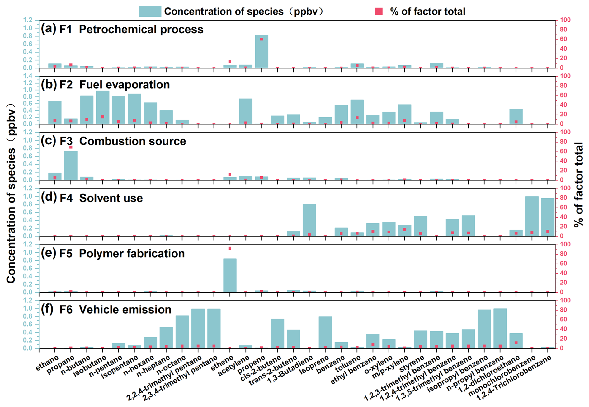
To ascertain the optimal number of sources, 20 iterations with varying random seeds were conducted to evaluate the stability of the Q value across solutions ranging from 3 to 10 factors. A 6-factor solution was selected as the rate of Q value reduction significantly diminished beyond this point, and the model results remained interpretable. The Q (true) $/$ Q (robust) value of 1.23 fell within the acceptable range of <1.5 (Hui et al., 2020), while the Q (robust) $/$ Q (theoretical) value of 1.1 indicated proximity to 1. The standardized residuals for each factor ranged from −3 to 3, demonstrating a satisfactory fit between the model predictions and observed data. The six sources identified using the PMF model are as follows: petrochemical process (PP), fuel evaporation (FE), combustion source (CS), solvent use (SU), polymer fabrication (PF) and vehicle emission (VE). The source profiles are illustrated in Fig. 5.

Factor 1 exhibited the highest concentration of propylene (60.60 %), suggesting its predominant source is local petrochemical processes. This finding aligns with previous studies that link propylene emissions to petrochemical activities in industrial zones (Washenfelder et al., 2010; Ragothaman and Anderson, 2017). Therefore, Factor 1 was determined to be PP. Factor 2 was characterized mainly by C₂–C₅ alkanes (47 %) and toluene (13.68 %); they are typical components of gasoline and diesel (Mu et al., 2023). Thus, Factor 2 is defined as a FE.

Factor 3 had a high percentage of propane (69.36 %), ethene (12.17 %) and ethane (5.12 %), which conformed to the emission characteristics of CS (Song et al., 2021; Chen et al., 2024). The relative contribution rate of aromatic hydrocarbons in Factor 4 reached 69.12 %. Currently, aromatic hydrocarbons are widely used as solvents in industrial production (Zhang et al., 2021; Mukhamatdinov et al., 2020). Factor 4 was defined as SU.

Factor 5 was primarily characterized by ethene (92.59 %), with its concentration far exceeding that of other species. It indicated that its source was closely related to the polymer manufacturing processes commonly found in nearby production facilities. Previous studies had identified ethene as a major pollutant associated with such industrial activities (Burdett and Eisinger, 2017). Therefore, Factor 5 was identified as originating from PF. Factor 6 was characterized by relatively high proportions of C₄–C₆ alkanes (37.63 %) and 1,2-dichloroethane (12.01 %), which are important indicators of VE (Song et al., 2021; Chen et al., 2024).

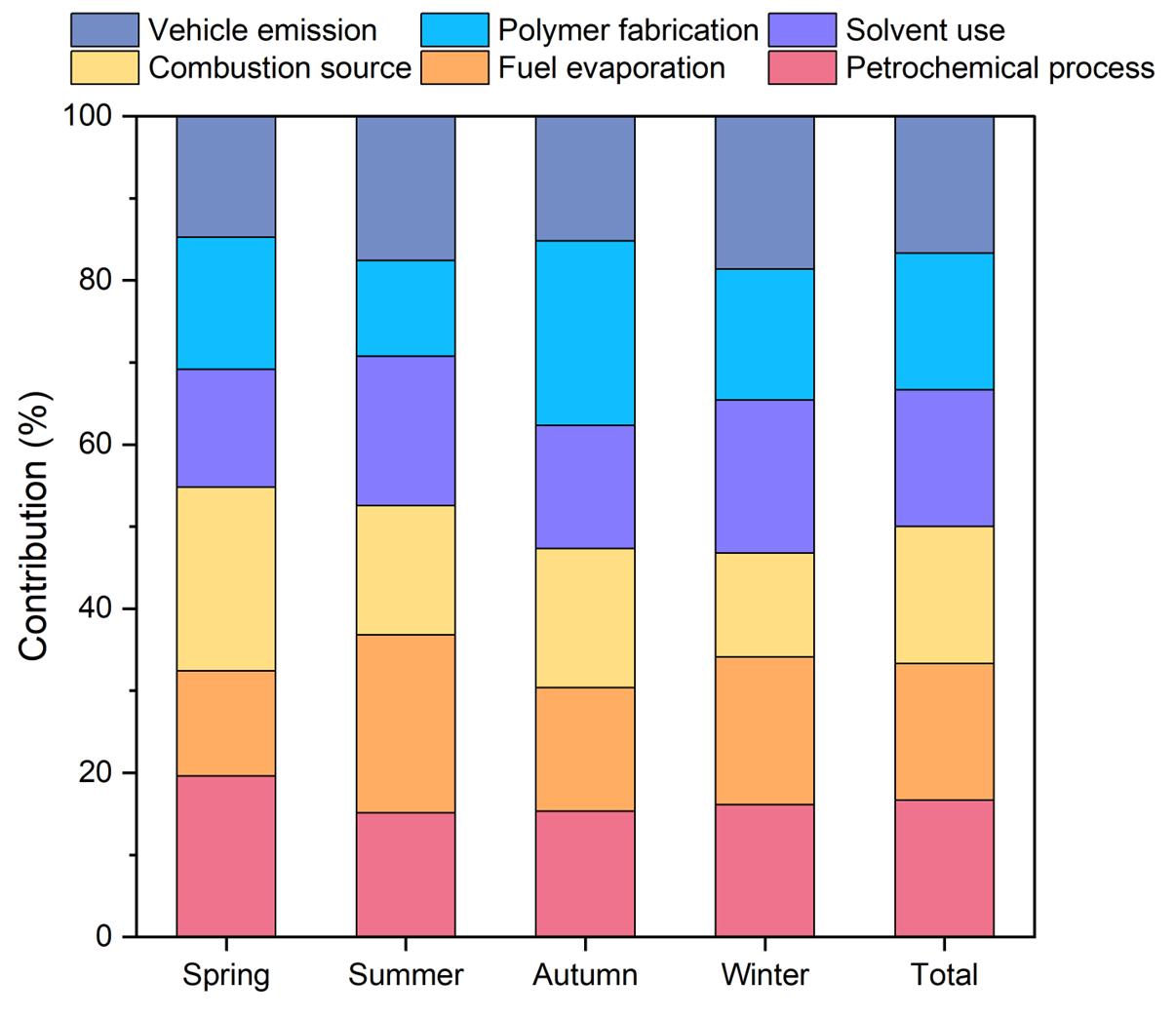
The PMF analysis revealed distinct temporal patterns in source contributions to VOC emissions throughout the study period (Fig. 6). On an annual basis, CS and FE emerged as the primary contributors, accounting for 16.94 % and 16.89 % of total VOC emissions, respectively. The remaining sources exhibited comparable contributions, SU (16.56 %), PF (16.54 %), VE (16.54 %) and PP (16.52 %), indicating a relatively balanced distribution of emission sources in the industrial park.

Figure 5 Source profiles calculated using the PMF model in site C.

3.3.2 Seasonal variation and contributing factors of VOC source distribution

Seasonal analysis unveiled significant temporal variations in source contributions (Fig. 6). During spring, CS dominated the VOC emissions with a 22.39 % contribution, followed by PP (19.59 %), PF (16.07 %) and VE (14.76 %), while FE showed a relatively lower contribution of 12.83 %. This pattern shifted notably in summer, where FE became the predominant source (21.68 %), accompanied by substantial contributions from SU (18.21 %) and VE (17.59 %). The autumn period witnessed PF emerging as the primary contributor (22.47 %), with CS maintaining a significant presence (16.95 %). Winter emissions were primarily attributed to VE (18.64 %), SU (18.61 %) and FE (18.02 %).

The observed seasonal variations align with regional industrial activities and meteorological conditions. The pronounced CS contributions during spring coincide with increased biomass burning activities across industrial parks in China, corroborating findings from previous studies (Yang et al., 2023; Yao et al., 2021; Chen et al., 2022). The elevated FE contributions in summer can be attributed to enhanced fuel volatilization under high temperatures characteristic of the Yangtze River Delta region, subsequently promoting O₃ formation (Xu et al., 2023). The autumn dominance of PF emissions reflects the operational patterns of polymer manufacturing facilities, while the significant winter contribution from VE aligns with previously documented patterns of vehicular emissions in Shanghai's urban areas (Liu et al., 2021; Wang et al., 2022).

Figure 6 Influence of various sources on atmospheric VOCs across different seasons.

3.4 Quantitative assessment of source-specific contributions to O₃ formation

The integrated PMF-SHAP framework was employed to quantitatively evaluate the source-specific contributions to O₃ formation in the Jinshan industrial complex during 2021–2023. Note that SHAP-derived source contributions are derived from the PMF-resolved source profiles (g matrix), not site-level TVOC data. This integrated approach directly links emission sources to O₃ impacts. Through the coupling of XGBoost-SHAP modeling with corresponding SHAP values, we systematically assessed the relative importance of various emission sources in driving O₃ pollution dynamics (Fig. 7). The analysis revealed that SU and FE were the predominant contributors to O₃ formation, exhibiting SHAP values of 3.00 and 2.77, respectively. This finding underscores the critical role of solvent usage and fuel-related emissions in industrial processes as primary drivers of O₃ generation. CS demonstrated moderate influence with a SHAP value of 2.19, followed by VE (1.92) and PP (0.55), while PF exhibited the lowest impact (0.16). These results emphasize the particular significance of SU and FE in O₃ pollution control strategies within industrial contexts.

To quantify the contribution of VOC sources identified by PMF to O₃ formation, we integrated the mass contributions of VOCs from specific sources with their respective maximum incremental reactivity (MIR) values (Carter, 2010; Venecek et al., 2018). Subsequently, we employed ozone formation potential (OFP) to assess the relative contributions of different VOCs to O₃ generation. The OFP quantification of PMF-resolved sources (Fig. S5) aligns robustly with SHAP-derived source prioritization, validating the scientific coherence of the PMF framework. SU exhibits the highest OFP contribution (32.20 µg m⁻³), driven by its dominant aromatic constituents (m-/p-xylene: 14.55 %, MIR = 5.47 gO₃/gVOC; ethyl benzene: 10.57 %, MIR = 3.11 gO₃/gVOC; o-xylene: 9.28 %, MIR = 7.17 gO₃/gVOC) whose combined reactivity (MIR-weighted OFP = 14.85 µg m⁻³) amplifies its ozone-driving potential despite moderate mass abundance (34.40 % of total VOCs). In contrast, FE (26.3 µg m⁻³) demonstrated a higher OFP, driven by the substantial mass proportion of C₂–C₅ hydrocarbons (68.15 %) and their high mean concentration (11.81 µg m⁻³). The SHAP value (3.00) confirmed its disproportionate influence on O₃ formation relative to its mass contribution. Additionally, VE (10.10 µg m⁻³) exhibited the lowest OFP, primarily due to the low reactivity of 1,2-dichloroethane (12.50 % by mass, MIR = 0.23). The SHAP value (1.92) reflected its limited photochemical impact. To contextualize the ML-derived findings within established regional photochemistry, we explicitly reconcile our SHAP-based source rankings (SU > FE > CS) with empirical kinetic modeling approach (EKMA) studies specific to the Shanghai. The dominance of solvent use (SU) and fuel evaporation (FE) sources aligns with EKMA analyses demonstrating VOC-limited regimes in Shanghai's industrial corridors (Zhang et al., 2024), where reactive aromatics (m-/p-xylene) and short-chain alkenes (propylene, 1,3-butadiene) drive >70 % of incremental reactivity.

The seasonal decomposition of source contributions through SHAP analysis demonstrated strong concordance with PMF-derived temporal patterns (Fig. 8). CS emerged as the dominant contributor during spring (30.51 %), while summer was characterized by substantial contributions from FE (27.25 %) and SU (24.48 %). The autumn period was dominated by PF emissions (27.83 %), whereas SU showed peak influence during winter (31.23 %). This temporal heterogeneity in source contributions, particularly the significant TVOC emissions associated with Site C, provides crucial insights for targeted O₃ management strategies.

Contrary to conventional CTM-based studies emphasizing combustion sources (CS) as primary O₃ drivers, our ML–PMF–SHAP integration identifies solvent use (SU, SHAP = 3.00) and fuel evaporation (FE, SHAP = 2.77) as dominant contributors. This shift highlights industrial process-specific emissions (e.g., aromatic solvents, light alkanes) as critical O₃ precursors in petrochemical zones, challenging broad regional assumptions. Site C exhibits a unique negative SHAP-O₃ correlation despite high VOC loads. We attribute this to rapid NO titration from proximate NO_x-rich plumes (e.g., gas stations, port activities), suppressing local O₃ while fueling downwind formation (>5 km) as air masses age into VOC-limited regimes – a micro-scale dynamic unresolvable by traditional PMF-OFP methods. SHAP quantifies disproportionate O₃ impacts unconstrained by VOC mass. For example, SU contributes only 34.40 % of total VOCs but drives 32.20 µg m⁻³ OFP due to high-reactivity aromatics (e.g., o-xylene, MIR = 7.17 gO₃ $/$ gVOC), whereas FE's higher mass (68.15 % alkanes) yields lower OFP (26.3 µg m⁻³) but amplified SHAP influence via spatial persistence. These insights establish a paradigm for facility-scale O₃ control, prioritizing SU/FE reductions over combustion sources in coastal industrial clusters. These findings have significant implications for policy development and implementation. The results suggest that regulatory attention should prioritize emission controls around Site C, with particular emphasis on seasonal variation in source contributions. Implementation of season-specific control strategies, especially targeting predominant sources during high-O₃ periods, would optimize the effectiveness of O₃ pollution mitigation efforts in industrial areas.

Figure 7 Mean SHAP values for six pollution sources affecting ozone levels.

Figure 8 Proportional contributions of six pollution sources to ozone levels, represented by SHAP values across different seasons.

4 Conclusions

This study presents a novel methodological framework for quantifying VOC contributions to O₃ formation in industrial park environments, integrating advanced ML techniques with traditional source apportionment methods. Through the synergistic combination of ML algorithms, SHAP interpretation and PMF modeling, we have developed a robust analytical approach that provides unprecedented spatial and temporal resolution in source identification and contribution assessment.

The investigation revealed distinct patterns in VOC–O₃ relationships, with solvent utilization and fuel evaporation emerging as primary drivers of O₃ formation in the industrial complex. The XGBoost model demonstrated superior predictive performance (R²=0.644) among the evaluated ML algorithms, while SHAP analysis enabled precise quantification of source-specific contributions. The PMF analysis further delineated six distinct emission sources, exhibiting pronounced seasonal variations in their relative contributions to O₃ formation.

Notably, combustion sources dominated spring emissions (30.51 %), while fuel evaporation (27.25 %) and solvent use (24.48 %) were predominant during summer months. This temporal heterogeneity in source contributions underscores the necessity for season-specific control strategies tailored to industrial operational patterns and meteorological conditions. The significant influence of Site C, characterized by diverse industrial activities, highlights the importance of targeted emission controls in areas with complex source profiles.

These findings provide crucial insights for evidence-based policy development in industrial air quality management. The methodology established herein offers a powerful tool for rapid source identification and precise contribution quantification, enabling the implementation of targeted control strategies at facility-level resolution. While our integrated PMF-ML-SHAP framework advances high-resolution source attribution for industrial O₃ formation, three key limitations warrant consideration: the 1 km × 1 km spatial resolution, though unprecedented for facility-scale analysis, may not resolve sub-facility emission hotspots (e.g., individual storage tanks or pipeline leaks), necessitating future integration of drone-based hyperspectral sensors or stack-level monitors for hyperlocal validation. Furthermore, reliance on hourly GC-FID measurements could underestimate fast-reacting alkenes (e.g., propylene, isoprene) with atmospheric lifetimes <2 h; real-time proton-transfer-reaction mass spectrometry (PTR-MS) would enhance temporal resolution for such compounds. Lastly, while optimized for Shanghai's coastal petrochemical environment – characterized by high humidity (>75 %), sea–land breezes (3–5 m s⁻¹) and reactive aromatic–alkene mixtures – the framework's efficacy requires validation in inland/arid industrial regions with distinct meteorology (e.g., lower humidity, weaker advection) and emission profiles (e.g., solvent-dominated manufacturing clusters). These constraints highlight inherent trade-offs between resolution and practicality but do not invalidate the framework's utility for targeted O₃ management in complex industrial zones. Future research directions should focus on expanding the temporal and spatial coverage of monitoring networks and exploring the application of this framework across diverse industrial settings to enhance its generalizability and predictive capabilities.

Appendix A: Acronym glossary

CatBoost	Category Boosting
CS	combustion sources
CSEM	cross-stacked ensemble learning model
CTMs	chemical transport models
DTR	Decision Tree Regression
EF	error score
FE	fuel evaporation
GC-FID	gas chromatography–flame ionization detector
GC-FID/MS	gas chromatography–flame ionization detector and mass spectrometry
LightGBM	Light Gradient Boosting Machine
MAE	mean absolute error
MDL	minimum detection limit
MDLs	method detection limits
MIR	maximum incremental reactivity
ML	machine learning
NOx	nitrogen oxides
O3	ozone
OFP	ozone formation potential
PF	polymer fabrication
PMF	positive matrix factorization
PP	petrochemical processes
RF	Random Forest
RMSE	root mean squared error
SHAP	SHapley Additive exPlanations
SU	solvent use
SVM	Support Vector Machine
SVR	Support Vector Regression
TVOCs	total volatile organic compounds
VE	vehicle emissions
VOCs	volatile organic compounds
XGBoost	Extreme Gradient Boosting