Impact of present aircraft NO_x and aerosol emissions on atmospheric composition and climate: results from a model intercomparison

Aircraft emissions of nitrogen oxides (NO_x= NO + NO₂), aerosols, and aerosol precursors provide a non-negligible contribution to the climate impact of air traffic, and the uncertainty in their climate Effective Radiative Forcing (ERF) remains significant. This study presents results from a new model intercomparison of the impact of aircraft emissions involving five state-of-the-art global models including both tropospheric and stratospheric chemistry. Aircraft NO_x increases ozone photochemical production in the free troposphere throughout the year and decreases ozone chemical loss in the high-latitude lowermost stratosphere during spring–early summer. The models generally agree on the spatial pattern of NO_x, ozone, and hydroxyl radical (OH) responses. The NO_x net ERF is systematically positive with a model mean of 18.3 mW m⁻², ranging from 9.4 to 24.5 mW m⁻² among the different models. This net NO_x forcing is reduced by 35 % and 43 % accounting for the negative forcing arising from the formation of nitrate and sulfate particles, respectively. Estimates of the aerosol direct ERF are systematically negative and range between −6.5 and −17.8 mW m⁻², compensating most of the net NO_x ERF albeit with noticeable intermodel differences arising from the diversity in aerosol parameterizations. This work shows encouraging results regarding our confidence in aviation NO_x-induced ozone response because of a good model agreement. To a lesser extent, some similarities in the results regarding aerosols are also encouraging, given the few existing model intercomparisons on this topic. However, the results also highlight areas where further modeling experiments are needed, both with more models and with dedicated sensitivity simulations to further understand the factors giving rise to the spread in model estimates of aviation emission impacts on atmospheric composition and climate.

1 Introduction

Air traffic emissions play a non-negligible role in climate change (Arias et al., 2021; Szopa et al., 2021) and air quality (e.g. Prashanth et al., 2022). As a long-lived species, carbon dioxide (CO₂) is the main climate forcer in the long term, and its radiative effect is reasonably well-quantified (Boucher et al., 2021). Additionally, the radiative effect from aviation non-CO₂ emissions has recently been evaluated to account for two-thirds of the total aircraft effective radiative forcing (ERF) from 1940 until 2018, but is characterized by uncertainties 8 times greater than for CO₂ (Lee et al., 2021). Consequently, when estimating the benefit of aviation mitigation strategies, it is crucial to quantify and constrain both CO₂ and non-CO₂ effects.

Non-CO₂ emissions include a variety of chemically reactive gaseous and particulate compounds. The emitted species include sulfur dioxide (SO₂) forming so-called sulfate (SO₄) particles that tend to cool the surface by scattering the incoming solar radiation, and black carbon (BC) – or soot – particles that tend to warm the atmosphere by absorbing the incoming solar radiation. Aerosols also have an indirect effect on climate through aerosol-cloud interactions, but the large uncertainties do not allow for a robust estimate in the case of aviation. Among the non-CO₂ gaseous components, water vapor (noted hereafter as H₂O) is the most abundantly emitted species. Its injection into the dry lowermost stratosphere (LMS), where its lifetime is substantially longer than in the troposphere, induces a positive radiative forcing (Lee et al., 2021). H₂O, together with soot particles, also leads to the formation of contrail-cirrus, which is estimated to exert the largest individual contribution to positive RF, but with large uncertainty (e.g. Lee et al., 2021; Wilhelm et al., 2021). Another of the non-CO₂ effects from aviation, still surrounded by a large uncertainty, is induced by nitrogen oxides (NO_x= NO + NO₂), a necessary catalyzer for tropospheric ozone (O₃) production. Though emitted in lesser quantities from aircraft than from other transport modes (e.g. Righi et al., 2023, Fig. 1), the injection directly into the free troposphere makes high-altitude NO_x emissions more efficient in producing ozone (e.g. Finney et al., 2016). It is linked both to the longer NO_x lifetime in this region, and its lower NO_x background. Compared to lightning NO_x emissions that likely represent 2–8 TgN yr⁻¹ (Schumann and Huntrieser, 2007), aviation NO_x emissions are not negligible as they are currently near 1 TgN yr⁻¹, i.e. potentially up to 50 % of the lightning emissions. Ozone has been confirmed as one of the main greenhouse gases linked with anthropogenic activities (Stevenson et al., 2013).

Earlier studies show that the main ozone perturbation induced by aircraft NO_x is located in the vicinity of the tropopause (e.g. Brasseur et al., 2016) where changes in ozone cause the most important positive RF (Riese et al., 2012). Changes in NO_x and ozone further modify the atmospheric oxidizing capacity by promoting the formation of the hydroxyl radical (OH), impacting atmospheric chemistry and particularly methane oxidation. The increased abundance of OH in the troposphere causes the reduction of atmospheric methane (CH₄) lifetime, which induces a negative radiative forcing over about a decade following the emission, thus partly counteracting the initial ozone-induced warming effect. Since methane is an ozone precursor in the troposphere and a water vapor precursor in the stratosphere, its increased sink in the short term decreases the production of these two species during the decade following the emission, thus increasing the cooling term due to methane destruction (e.g. Myhre et al., 2011). Through the production of tropospheric OH, aircraft NO_x also promotes the formation of sulfate and nitrate (NO₃) particles (because of an enhanced oxidation of SO₂ and NO_x), thus acting as an additional cooling factor (Brasseur et al., 2016; Terrenoire et al., 2022). Based on the existing literature, Lee et al. (2021) estimated the net aviation NO_x impact to exert an effective radiative forcing (ERF) of 17.5 [0.6–28.5] mW m⁻² for the year 2018, resulting from a positive ERF from short-term ozone of 49.3 [33–76] mW m⁻² and a negative ERF from long-term methane decrease of −34.9 [−65 to −25] mW m⁻², thus highlighting high uncertainties for both processes. However, Lee et al. (2021) did not account for the NO_x effect on aerosol formation, as they point out the limited number of studies on this topic and the large associated uncertainties. Also, the assessment by Lee et al. (2021) is based on an important set of modelling studies which have been harmonised regarding time periods and aircraft emissions in order to account solely for inter-model differences in both chemistry and radiation. In this study we revisit the aircraft NO_x perturbations on chemistry and climate based on the latest generation of five global chemistry-climate/transport models and on a common modelling protocol regarding surface and aircraft emissions and time period covered. This further reduces the need for harmonisation of the model results as a post-treatment and allows to focus on the inter-model differences in the treatment of chemistry and dynamics.

Several studies have conducted model intercomparisons to more robustly evaluate the impact of aircraft emissions on atmospheric composition, and its consequences for climate (Hoor et al., 2009; Hodnebrog et al., 2011, 2012; Olsen et al., 2013; Søvde et al., 2014; Brasseur et al., 2016). All these studies accounted for short-term ozone perturbation, methane perturbation, and long-term O₃ and stratospheric H₂O perturbations. In the framework of the QUANTIFY project (Quantifying the Climate Impact of Global and European Transport Systems), Hoor et al. (2009) found a net RF of 2.9 ± 2.3 mW m⁻² for the year 2003. Søvde et al. (2014) obtained a range of 1–8 mW m⁻² for the year 2006 (4–8 mW m⁻² without the most sensitive model regarding methane loss), with the REACT4C (Reducing Emissions from Aviation by Changing Trajectories for the benefit of Climate) emission inventory (Matthes et al., 2012). In the framework of the ACCRI program, Brasseur et al. (2016) derived a range of 6–36.5 mW m⁻² (resp. −12.3 to −8 mW m⁻²) concerning the short-term ozone response (resp. methane lifetime decrease) for the year 2006, with only one model accounting for the long-term ozone/H₂O responses. These estimates remain characterized by a high uncertainty due to the differences between models (with a standard deviation greater than 50 %), and/or due to chemical processes not accounted for, as in Brasseur et al. (2016). The latter study also shows the impact of aircraft on several gaseous and aerosol species, but not necessarily with the same models, thus limiting the interpretation of the results. Last, the aviation impact on nitrate aerosol is relatively new in the literature, and most of all, there is no model intercomparison regarding its perturbation due to aircraft emissions.

Here, we present results from a new multi-model intercomparison conducted under the framework of the EU project ACACIA (Advancing the Science for Aviation and Climate). Simulations were performed with five up-to-date global chemistry-climate models (CCMs) or chemistry-transport models (CTMs) with a common simulation protocol, notably imposing the recent inventories used by CMIP6 for anthropogenic surface and aircraft emissions (Hoesly et al., 2018; Gidden et al., 2019), and for biomass burning emissions (van Marle et al., 2017), using the same prescribed sea-surface temperatures (SSTs) and surface methane concentrations, and nudging or forcing the horizontal wind speeds with reanalysis output (ERA-Interim or MERRA-2). A companion paper is dedicated to the assessment of the model baseline performance using in-situ aircraft observations (Cohen et al., 2025); in the present study, the focus is on the effect of aircraft NO_x and, secondarily, aerosols and aerosol precursor emissions on atmospheric composition and associated radiative forcings of climate. The objectives of this study are (1) to provide an overview of the methodology of the harmonized multi-model study, (2) to present aviation-induced changes in the concentration of reactive species and the extent to which models agree, as well as specific differences between individual models, including an evaluation of the linearity of aviation induced effects. Thanks to the ancillary variables provided by two of the models, our intercomparison is the first to suggest an explanation for the pattern of ozone changes in response to aircraft NO_x. Finally, (3) to provide estimates of the radiative effects of the simulated aviation-induced ozone, methane, and aerosol changes.

Section 2 describes the models, input data, and methods, while Sect. 3 shows the changes in atmospheric composition due to aviation emissions as simulated by the models. Section 4 provides the associated radiative forcing of climate. In Sect. 5, we draw the conclusions of the current study.

2 The model intercomparison

2.1 Participating global models

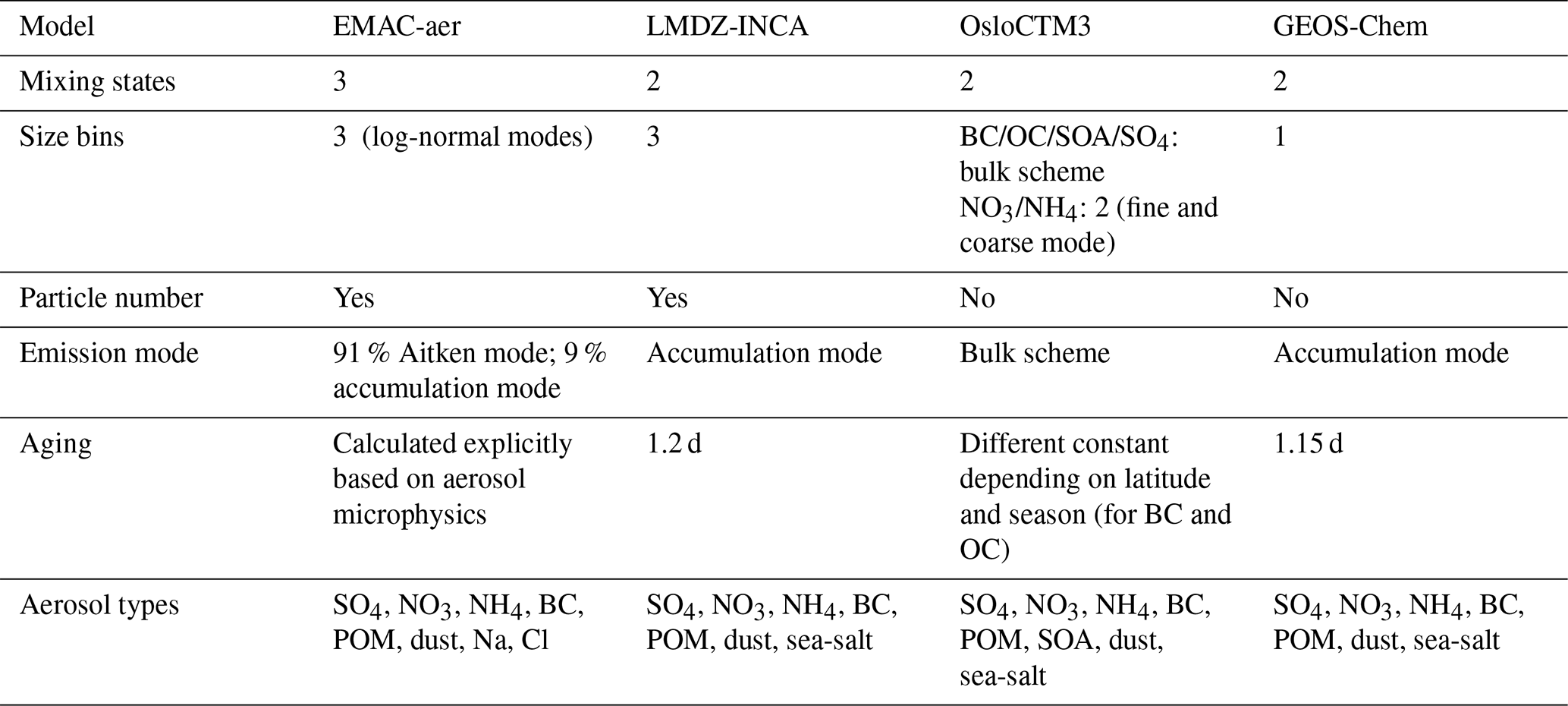
Table 1 summarizes the general characteristics of the participating models, and Table 2 summarizes the aerosol parameterization for the models that provide aerosol variables. For each model described in Table 2, the pairs of mixing states correspond to the hydrophilic or hydrophobic state (with hydrophobic particles that can evolve into hydrophilic through aging processes), and the three mixing states for EMAC-aer also include a mixed-particles category. It applies to both black carbon and organic carbon.

Table 1 Description of the participating models. The acronyms and abbreviations are explained here. In the first column, the abbreviations Horiz., Vert., Hom., Phot., Het., and BVOC denote horizontal, vertical, homogeneous, photolytic, heterogeneous, and biogenic volatile organic compounds respectively, and GCM stands for General Circulation Model. Among the aerosol categories, SO₄, NO₃, NH₄, BC, OC, POM, Cl, and Na represent sulfate, nitrate, ammonium, black carbon, organic carbon, primary organic matter, chlorine, and other marine components (mainly sodium), respectively. In the references, G2001 represents Grewe et al. (2001), PR92 and P1997 represent Price and Rind (1992) and Price et al. (1997), O2010 represents Ott et al. (2010), P1998 represents Pickering et al. (1998), and M2012 represents Murray et al. (2012).

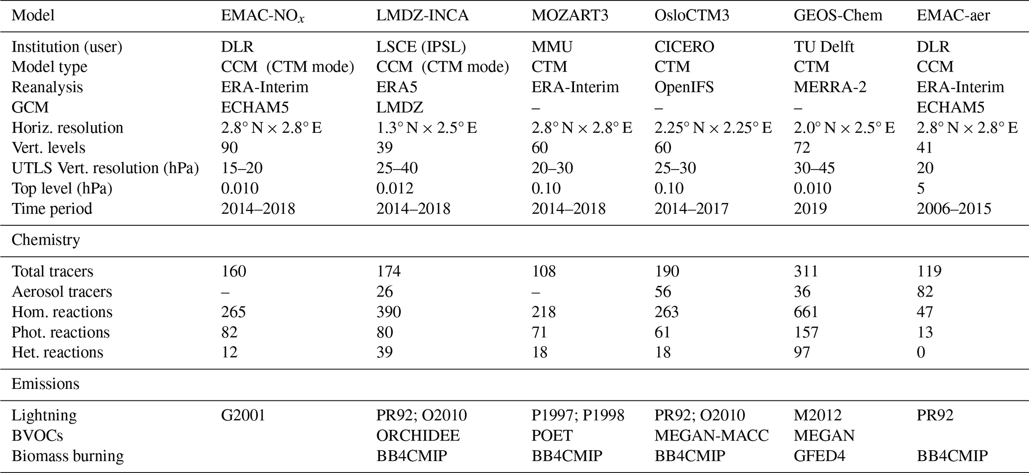
Table 2 Description of the aerosol parameterization in the four models providing aerosol output.

2.1.1 EMAC

The ECHAM/MESSy Atmospheric Chemistry (EMAC) model is a numerical chemistry and climate simulation system that includes sub-models describing tropospheric and middle atmosphere processes and their interaction with oceans, land, and human influences (Jöckel et al., 2010). It uses the second version of the Modular Earth Submodel System (MESSy2) to link multi-institutional computer codes. As described in Jöckel et al. (2016), MESSy is a software package providing a framework for a standardized, bottom-up implementation of Earth system models with flexible complexity (Modular Earth Submodel System). The core atmospheric model is the 5th generation European Centre Hamburg general circulation model (ECHAM5: Roeckner et al., 2006). The physics subroutines of the original ECHAM code have been modularized and reimplemented as MESSy submodels and have continuously been further developed. Only the spectral transform core, the flux-form semi-Lagrangian large-scale advection scheme, and the nudging routines for Newtonian relaxation remain from ECHAM. For the present study, we applied EMAC in two different configurations, for NO_x and aerosol. Hereafter, we refer to them as EMAC-NO_x and EMAC-aer, respectively. EMAC-NO_x is based on MESSy version 2.55.2 in the T42L90MA-resolution, i.e. with a spherical truncation of T42 (corresponding to a quadratic Gaussian grid of approximately 2.8 by 2.8° in latitude and longitude) with 90 vertical hybrid pressure levels up to 0.01 hPa, whereas EMAC-aer is based on MESSy version 2.54.0 in the T42L41DLR-resolution, with 41 levels up to 5 hPa (see Righi et al., 2023, for further details). In ECHAM5, the nudging applies to vorticity, temperature, logarithm of the surface pressure, and divergence with a relaxation time being 6, 24, 24, and 48 h respectively. The NO_x configuration was run in the so-called Quasi Chemistry-Transport Model mode (QCTM: Deckert et al., 2011) enabling binary identical simulations with respect to atmospheric dynamics, so that perturbations in chemistry can be detected with a high signal-to-noise ratio. This mode was not used for the aerosol configuration, since this also includes aerosol-cloud interactions which are not compatible with this mode. Both model setups comprised the Module Efficiently Calculating the Chemistry of the Atmosphere (MECCA) used for tropospheric and stratospheric chemistry calculations with the possibility of extending to the mesosphere and oceanic chemistry (Sander et al., 2019). Reaction mechanisms include ozone, methane, HO_x, NO_x, NMHCs, halogens, and sulfur chemistry for EMAC-NO_x, while a simplified chemical mechanism was used in EMAC-aer, comprising the NO_x–HO_x–CH₄–CO–O₃ chemistry and the tropospheric sulfur cycle. Radiative transfer calculations are performed using the submodel RAD (Dietmüller et al., 2016). EMAC-aer uses the submodel MADE3 (Kaiser et al., 2019) for aerosol microphysics.

2.1.2 LMDZ-INCA

The LMDZ-INCA global chemistry-aerosol-climate model couples online the LMDZ general circulation model (Laboratoire de Météorologie Dynamique, version 6: Hourdin et al., 2020) and the INCA model (INteraction with Chemistry and Aerosols, version 6: Hauglustaine et al., 2004). In the present configuration, the model includes 39 hybrid vertical levels extending up to about 80 km. The horizontal resolution is 1.25° in latitude and 2.5° in longitude. INCA initially included a state-of-the-art CH₄–NO_x–CO–NMHC–O₃ tropospheric photochemistry (Hauglustaine et al., 2004; Folberth et al., 2006). Ammonia and nitrate aerosols are considered as described by Hauglustaine et al. (2014). The model has been extended to include an interactive chemistry in the stratosphere and mesosphere. Chemical species and reactions specific to the middle atmosphere were added to the model. A total of 31 species were added to the standard chemical scheme, mostly belonging to chlorine and bromine chemistry, with 66 gas-phase reactions and 26 photolytic reactions (Terrenoire et al., 2022; Pletzer et al., 2022). In this study, meteorological data from the European Center for Medium-Range Weather Forecasts (ECMWF) ERA5 reanalysis have been used to constrain the GCM meteorology. The relaxation of the GCM winds towards ECMWF meteorology is performed by applying at each time step a correction term to the GCM zonal and meridional wind components with a relaxation time of 3.6 h. The ECMWF fields are provided every 6 h and interpolated onto the LMDZ grid. The lightning NO_x (LNO_x) parameterization is updated from Jourdain and Hauglustaine (2001). The flash frequency is determined by the cloud-top height and the surface type (land or ocean), following Price and Rind (1992). As in Cohen et al. (2023), the number of flashes is rescaled to the global mean frequency of 46.3 flash s⁻¹ derived from Lightning Imaging Sensor and Optical Transient Detector (OTD/LIS: Cecil et al., 2014). The vertical profile of LNO_x emissions follows the parameterization in Ott et al. (2010).

2.1.3 MOZART3

Model for OZone And Related chemical Tracers, version 3 (MOZART3) is an offline, global chemical transport model, extensively evaluated (Kinnison et al., 2007) and used for a range of various applications (Liu et al., 2009; Wuebbles et al., 2011), including studies dealing with the impact of aviation emissions on atmospheric composition (Søvde et al., 2014; Skowron et al., 2015). The horizontal resolution used in this study is T42 (2.8° × 2.8°) and vertically the model domain spans 60 layers between the surface and 0.1 hPa. The transport of chemical compounds as well as the hydrological cycle is driven by the meteorological fields from ECMWF Interim 6 h reanalysis (ERA-Interim). The model reproduces detailed chemical and physical processes from the troposphere through the stratosphere. The chemical mechanism consists of 108 species, 218 gas-phase reactions, 71 photolytic reactions including the photochemical reactions associated with organic halogen compound, and 18 heterogeneous reactions involving four aerosol types: liquid binary sulfate, supercooled ternary solution, nitric acid tri-hydrate, and water-ice. The kinetic and photochemical data is based on the NASA/JPL evaluation (Sander et al., 2006). MOZART3 accounts for advection based on the flux-form semi-Lagrangian scheme (Lin and Rood, 1996), shallow and mid-level convection (Hack, 1994), deep convective routine (Zhang and McFarlane, 1995), boundary layer exchanges (Holtslag and Boville, 1993), or wet and dry deposition (Brasseur et al., 1998; Müller, 1992). The parameterization of NO_x emissions from lightning follows the assumption that the lightning frequency depends on the convective cloud top height and the ratio of cloud-to-cloud versus cloud-to-ground lightning depends on the cold cloud thickness (Price et al., 1997). The lightning NO_x emissions are distributed vertically through the convective column according to observed profiles based on Pickering et al. (1998). The lightning source is scaled to provide a total of 4.7 Tg N yr⁻¹, with daily and seasonal fluctuations based on the model meteorology. The patterns of lighting NO_x distribution in MOZART3 show a general agreement with LIS and OTD climatology datasets (Skowron et al., 2021).

2.1.4 OsloCTM3

OsloCTM3 is a global, offline chemical transport model, driven by 3-hourly meteorological forecast data from the ECMWF Open Integrated Forecast System (OpenIFS) model (Søvde et al., 2012). The model is run in its default horizontal resolution of 2.25° × 2.25° with 60 levels, the uppermost centered at 0.1 hPa. The OsloCTM3 treats comprehensive tropospheric and stratospheric chemistry (Berntsen and Isaksen, 1997; Stordal et al., 1985), as well as the main anthropogenic and natural aerosol species (sulfate, nitrate/ammonium, black carbon, primary and secondary organic aerosol, dust, and sea salt). The kinetics are based on JPL 2006 (Sander et al., 2006), while the photodissociation coefficients are calculated online using the Fast-JX scheme (Prather, 2009). The numerical integration of chemical kinetics is done by applying the Quasi Steady State Approximation (QSSA: Hesstvedt et al., 1978), using three different integration methods depending on the chemical lifetime of the species. The aerosol schemes are described in more detail in Lund et al. (2018a). Notably, 80 % of emitted BC is considered as hydrophobic and 20 % as hydrophilic, with an aging that consists of a constant rate depending on the region and the season (Lund and Berntsen, 2012). Large-scale advection is treated by the second-order moments (SOM) scheme (Prather, 1986), convective is based on Tiedtke (1989), and boundary layer mixing is based on Holtslag et al. (1990). Scavenging covers dry deposition, i.e. uptake by soil or vegetation at the surface, and washout by convective and large-scale rain (Søvde et al., 2012).

2.1.5 GEOS-Chem

GEOS-Chem is a chemistry-transport model with unified tropospheric-stratospheric oxidant-aerosol chemistry. The original gas-phase tropospheric oxidant model of GEOS-Chem is described by Bey et al. (2001). Aerosol chemistry, modeling the SO₄–NO₃–NH₄ system, is described by Park et al. (2004). The ISORROPIA II thermodynamic module is used for the aerosol model (Fountoukis and Nenes, 2007). Heterogeneous chemistry of nitrate aerosols is as described by Holmes et al. (2019). Aerosol hygroscopicity is modeled as described by Latimer and Martin (2019), and cloud water pH as described by Shah et al. (2020). The stratospheric chemistry model is described by Eastham et al. (2014). Emissions are implemented with the HEMCO module described by Keller et al. (2014). In this study, GEOS-Chem classic v13.3 is used, driven by the MERRA-2 reanalysis product (Gelaro et al., 2017). The model's “fullchem” configuration is used, without the optional extensions for aerosol microphysics and complex SOA modeling. Meteorology and emissions are for the year 2019. Timesteps are 10 min for transport and convection, and 20 min for chemistry and emissions. The model is spun-up with runs of 21 months at 4° latitude by 5° longitude, followed by 3 months at the final resolution. Lightning NO_x emissions are as described by Murray et al. (2012) to match OTD/LIS climatological observations of lightning flashes. Biogenic VOC emissions in GEOS-Chem are from the MEGAN v2.1 inventory of Guenther et al. (2012) as implemented by Hu et al. (2015). Leaf area indices (LAIs) used in MEGAN v2.1 are from the Yuan et al. (2011) MODIS product for 2005–2020. Dependence on CO₂ was added by Tai et al. (2013). Acetaldehyde emissions are from Millet et al. (2010). Biogenic non-agricultural ammonia sources are from GEIA (Bouwman et al., 1997). Emissions from open fires for individual years are from the GFED4.1s inventory.

2.2 Simulation set-up and emission inventories

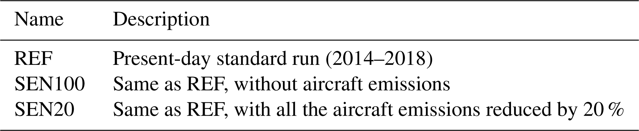
Each participating model (see Sect. 2.1) generated a set of simulations following a common protocol, based on a perturbation approach. As summarized in Table 3, each model provides at least one reference run including all emission sources and one run without any aviation emissions. To evaluate the linearity of the chemical and radiative response versus aviation NO_x emissions, three of the models (LMDZ-INCA, MOZART3, and OsloCTM3) also provided a run with all aviation emissions reduced by 20 % (then the difference with the reference run is rescaled up to 100 %). To provide a first estimate of the dependence on the NO_x background, an additional pair of runs was made by MOZART3 without lightning emissions. Three of the models (LMDZ-INCA, OsloCTM3, and GEOS-Chem) include aerosols, as well as EMAC in the EMAC-aer configuration.

Table 3 List of the different runs used in this study.

Each simulation is preceded by a 1-year spin-up and covers the period 2014–2018 (2014–2017 for OsloCTM3, and 2019 for GEOS–Chem), still considered as present-day when the protocol was designed. The wind horizontal velocities are directly taken from reanalyses for CTMs, and nudged toward a reanalysis for CCMs (ERA-I for EMAC, ERA5 for LMDZ-INCA) using a quasi-CTM mode, i.e. without any feedback between chemistry and dynamics (except for EMAC-aer).

The historical anthropogenic emissions are taken from the Community Emissions Data System inventory CEDS (Hoesly et al., 2018). Regarding aviation emissions (represented here by NO_x, SO₂, and BC), these files resolve aviation emissions with 25 vertical levels (or injection heights) from the surface up to 15 km. For EMAC-NO_x, LMDZ-INCA, MOZART3, and OsloCTM3, a correction (Thor et al., 2023) has been applied to the initial CEDS aviation emissions. Historical biomass burning emissions until 2014 are provided by the BB4CMIP inventory (van Marle et al., 2017), notably based on the Global Fire Emissions Database (GFED4s: van der Werf et al., 2017), followed by emissions prescribed in the SSP3-7.0 scenario until 2018 (Gidden et al., 2019). For these years (2015–2018), the differences between the scenarios remain small (less than 6 % for NO_x), as are the differences with the year 2014 in the CEDS inventory, given that the scenarios data sets have been harmonized with the historical data sets to ensure a consistent evolution before and after this transition year (further information for the year 2019 in GEOS-Chem is available below). Other emissions, primarily from natural sources, are not prescribed by the protocol and depend on the individual model. For example, biogenic volatile organic compounds (BVOC) emissions are calculated using a different module for each model. Lightning flash rate is parameterized using the commonly used scheme described in Price and Rind (1992) or Price et al. (1997) for most models (LMDZ-INCA, MOZART3, OsloCTM3, EMAC-aer), or similar for EMAC-NO_x (Grewe et al., 2001), and thus depends on the deep convection parameterization. The vertical distribution of LNO_x emission per flash is calculated using the scheme described in Ott et al. (2010) for LMDZ-INCA and OsloCTM3, or in its former version described in Pickering et al. (1998) for MOZART3.

Among the five models included in this paper, GEOS-Chem data is from pre-existing runs made for a different publication (Quadros et al., 2025) and is thus less consistent with the protocol. For this model, the monthly-averaged aircraft emissions are calculated from a list of all flights globally in the year 2019 provided by Flightradar24, as described by Quadros et al. (2022). For each combination of aircraft type, origin and destination in the database, 3-D gridded fuel burn is calculated using a time-in-mode approach for landing-and-takeoff operations (Stettler et al., 2011) and the Base of Aircraft Data (BADA) 3.15 aircraft performance model for climb, cruise and descent phases of flight (Mouillet, 2019). Great-circle trajectories between airports are used, with a lateral inefficiency factor based on Seymour et al. (2020) applied to adjust for additional fuel used in actual trajectories. Constant cruise flight levels are used, with aircraft type specific values determined from a subset of flights for which Flightradar24 provided altitude at the start of cruise, based on ADS-B data. Emissions are calculated alongside with fuel burn using the Boeing Fuel Flow Method 2 (Baughcum et al., 1996), the FOA4 method for non-volatile particulate matter (ICAO, 2020), and data from the International Civil Aviation Organization (ICAO) Engine Emissions Databank (ICAO, 2021).

The difference between Flightradar24 and CEDS emissions is well visible in the maps shown in Fig. S9 in the Supplement, with less NO_x emitted in West hemisphere and more in East hemisphere with Flightradar24. In terms of altitude, Fig. S10 shows a continuum in the vertical distribution in CEDS emissions (at 9–11 km) but two distinct peaks with Flightradar24, the most important at 10–11 km (as with CEDS) and a secondary peak at 8–9 km, lower than most emissions in CEDS. Also, the runs concern only the year 2019. As only three models included aerosol chemistry, and as the complexity of the aerosol representation is substantially different through the models, we also added the aerosol output from the EMAC aerosol-climate model published in Righi et al. (2023), called EMAC-aer in the present study. It has to be noted that the latter's experimental setup is substantially different, as it spans over 10 years (2006–2015) with emissions taken constantly at the same level as 2015 (from the SSP2 scenario), and as meteorology is influenced by atmospheric chemistry. To minimize the influence of interannual variability, we average the output over the 10 years of simulation.

Apart from the current study, it is worth mentioning that other tests were designed by the same common protocol. More runs have been made available to assess specifically the present-day impact of aviation NO_x on aerosols (Bellouin et al., 2026) by reducing only NO_x emissions, and the impact of future aviation emissions (Staniaszek et al., 2025).

2.3 Methodology

The requested monthly output from the 5 participating models is used to derive 5-year averages for each calendar month and for the whole year. Following the perturbation approach, we calculate the chemical composition responses as the difference between the reference run and the run without aviation emissions. For the runs with aviation emissions reduced by 20 %, we apply a factor of 5 to the difference in order to make it comparable to the 100 % reduction case.

The aviation emissions provided as output by the models can be slightly different for two reasons. First, the regridding of the emission files to the model native resolutions, which are all different. Second, the differences in the simulation years. For this purpose, we apply a rescaling factor to each model result to ensure the same amount of aircraft emissions. For a given model M, this factor is calculated as the R_M ratio following Eq. (1):

$$\begin{array}{}\text{(1)}& R_{\mathrm{M}}=E_{\mathrm{INCA}}\left({\mathrm{NO}}_x\right)/E_{\mathrm{M}}\left({\mathrm{NO}}_x\right)\end{array}$$

where E_M (NO_x) is the global aviation NO_x emissions averaged over the whole simulation period from the M model. E_INCA (NO_x) is the corresponding emission for the LMDZ-INCA model, with a value of 1.12 TgN yr⁻¹. This rescaling factor based on NO_x applies to the perturbation for all species, including aerosols and precursors. In most cases, this rescaling does not change the results significantly, as NO_x emissions range between 0.98 (EMAC-NO_x) and 1.12 TgN yr⁻¹ (LMDZ-INCA and MOZART3). We assume these differences to be small enough to neglect non-linearities in the chemical perturbation. One exception is GEOS-Chem, as its 2019 emissions are substantially higher (1.40 TgN yr⁻¹) than the average 2014–2018, so one has to keep in mind that linear rescaling is less adequate.

To derive the radiative impact of aviation-induced atmospheric composition changes, we use concentration-based kernels to calculate the stratospherically adjusted ozone RF and the instantaneous top-of-the-atmosphere RF due to aerosol–radiation interactions (Skeie et al., 2020; Samset and Myhre, 2011). To perform the RF calculations, ozone and aerosol data from all models were interpolated to the kernel resolution (2.25° × 2.25° and 60 vertical levels). For the calculation of the ozone column for each model, the air mass from OsloCTM3 was used, following the method in Skeie et al. (2020). The ozone RF calculations from the kernel have been found to compare favourably against offline radiative transfer model calculations in LMDZ-INCA and OsloCTM3. More generally, kernel-based estimates of ozone RF have been found to agree with those from full radiative transfer in previous applications (Lund et al., 2021). The response of the methane volume mixing ratio and the associated radiative forcing are calculated based on the modelled response in methane total lifetime for each simulation. It assumes, in addition to the methane oxidation by OH, a stratospheric sink characterized by a 120-year lifetime and a soil sink characterized by a 160-year lifetime. This calculation is combined with the methane feedback factor (referring to the CH₄ feedback on its own lifetime) and an emission non-steady state factor. This method is described in Berntsen et al. (2005), Hodnebrog et al. (2012) and Terrenoire et al. (2022). The methane reference mixing ratio is fixed at 1834 ppb. The methane feedback factor (f= 1.45) is taken as the model mean from a recent model intercomparison (Sand et al., 2023). We use a non-steady state factor to correct for the fact that due to its long lifetime, methane steady state is not reached, so assuming steady-state to derive the radiative forcing overstates the response (Grewe and Stenke, 2008). This non-steady factor was recently recalculated by Bellouin et al. (2026) to be 0.680 for present-day conditions. From this methane mixing ratio response, the methane RF is calculated using the simplified equation from Etminan et al. (2016). The indirect long-term ozone and stratospheric water vapour RFs are calculated based on the methane mixing ratio response adopting the normalized forcings from a recent model intercomparison (Sand et al., 2023). For long-term ozone we use a normalized forcing of 0.180 W m⁻² ppbCH${}_{\mathrm{4}}^{-\mathrm{1}}$ and, for stratospheric water, a normalized forcing of 0.058 W m⁻² ppbCH${}_{\mathrm{4}}^{-\mathrm{1}}$.

The calculated ozone and methane RFs are converted to ERFs based on the efficacies provided by Lee et al. (2021) (1.370 for the short-lived ozone forcing and 1.180 for the methane direct and indirect forcings). For aerosols, the kernel includes rapid adjustments for BC, thus representing the ERF, while the $\mathrm{ERF}/\mathrm{RF}$ ratio is assumed to be 1.0 for the scattering aerosols due to lack of other information (Lee et al., 2021).

3 Impact of aviation emissions on atmospheric composition

On the global scale, and from 150 hPa down to the surface, Table 4 synthesizes the global burden perturbation for several species, normalized by aircraft NO_x emissions. For a given species S, the mass perturbation in the global burden is calculated as follows:

$$\begin{array}{}\text{(2)}& \mathrm{\Delta }m\left(S\right)={\sum }_{i,j,k}\mathrm{\Delta }{\mathit{\rho }}_{i,j,k}\left(S\right)V_{i,j,k}\end{array}$$

where ${\mathit{\rho }}_{i,j,k}\left(S\right)$ is the mass density of the S species, and $V_{i,j,k}$ is the volume of the gridcell (i, j, and k being the spatial indexes). For gaseous species, in a gridcell characterized by a pressure P and a temperature T, the mass density is calculated from the volume mixing ratio X_S, as follows:

$$\begin{array}{}\text{(3a)}& \mathit{\rho }\left(S\right)={\displaystyle \frac{M_{S}P}{RT}}{X}_S\end{array}$$

where M_S is the molar mass of the S species, and R is the ideal gas constant.

For aerosols, the model output is provided as mass mixing ratios $X_S^{\prime }$. Thus, we derive the mass density similarly as Eq. (3a):

$$\begin{array}{}\text{(3b)}& \mathit{\rho }\left(S\right)={\displaystyle \frac{M_{\mathrm{air}}P}{RT}}{X^{\prime }}_S\end{array}$$

where M_air= 29 g mol⁻¹ is the molar mass for dry air.

Lastly, global aviation NO_x emissions ENO_x (in TgN yr⁻¹) are calculated by summing up the local emissions, expressed in molar concentration increase rate $\dot{n}$ (in mol m⁻³ s⁻¹), as follows:

$$\begin{array}{}\text{(4)}& {\mathrm{ENO}}_x=C{M}_N{\sum }_{i,j,k}{\dot{n}}_{i,j,k}\left({\mathrm{NO}}_x\right)V_{i,j,k}\end{array}$$

where M_N= 14 g mol⁻¹ is the molar mass of nitrogen, and C = 3.16 × 10⁻⁵ is a constant converting g s⁻¹ into Tg yr⁻¹.

3.1 Gas-phase chemistry

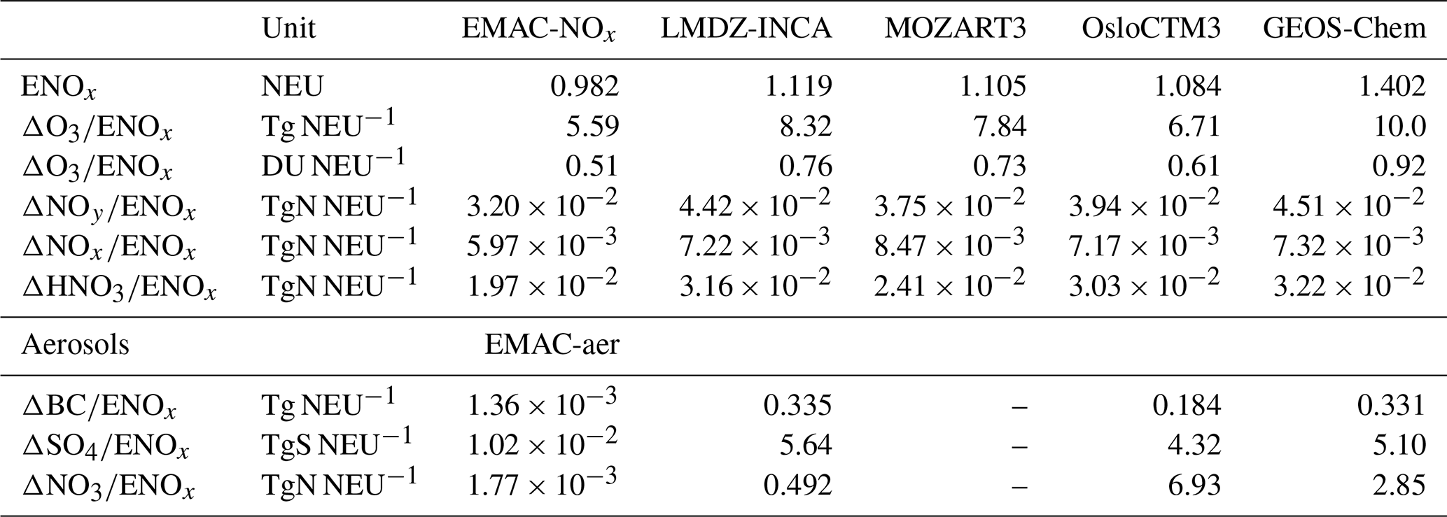
As seen in Table 4, the global NO_x perturbation ranges between 0.60 % (EMAC-NO_x) and 0.85 % (MOZART3) of the yearly emitted NO_x, in terms of nitrogen mass. Including the NO_x reservoir species, the NO_y perturbation spreads between 3.20 % and 4.51 %, the main contributor being nitric acid HNO₃ (1.97 %–3.22 %), representing ∼ 66 %–75 % of the NO_y perturbation. Normalized to 1 TgN yr⁻¹ of emitted NO_x (called hereafter NEU, for NO_x emission unit), the ozone perturbation ranges between 0.51 DU NEU⁻¹ (EMAC-NO_x) and 0.90 DU NEU⁻¹ (GEOS-Chem), i.e. between 5.6 and 10.0 TgO₃ NEU⁻¹. The values are similar between LMDZ-INCA and MOZART3. OsloCTM3 shows a higher mean sensitivity compared to EMAC-NO_x although the perturbation for EMAC-NO_x mixing ratio reaches higher values (as seen later, in Fig. 5), which is due to the lower altitude of the OsloCTM3 response (hence a greater mass perturbation) and to its wider vertical range. In comparison, Olsen et al. (2013) and Brasseur et al. (2016) present the ozone burden sensitivity in 2006 to the NO_x emissions from the Aviation Environmental Design Tool (AEDT) inventory from the Federal Aviation Administration (FAA), with a spread between 2.8 and 11.2 Tg NEU⁻¹ from both offline and online models, and 6.7, 9.0 and 11.2 Tg NEU⁻¹ from the three CTMs exclusively (respectively CAM5, CAM4, and GEOS-Chem). Compared to the current study (5.6–10.0 Tg NEU⁻¹), the inter-model range is similar. The ozone burden sensitivity is lower in our results than in these two studies, but the aviation NO_x emission is 36 % greater in 2014–2018 (1.119 NEU) than in 2006 (0.812 NEU, as shown in Table 2 from Brasseur et al., 2016), thus leading the chemical conditions closer to the NO_x-saturated regime. Last, in both studies, GEOS-Chem is characterized by the highest response, with a higher ozone sensitivity (11.2 Tg NEU⁻¹) than the current study (10.0 Tg NEU⁻¹).

Table 4 Ratios between the global burden perturbation and the NO_x annual emissions. The aviation NO_x emission unit (NEU) is defined here as 1 NEU = 1 TgN yr⁻¹.

3.1.1 Seasonal cycles in the UTLS

Figure 1 displays Hovmöller diagrams for several gaseous compounds. As the models can have different altitudes in the maximum ozone response to aviation NO_x emissions (as seen later for OsloCTM3 in Fig. 5), the vertical average is made between 150 and 350 hPa to capture as much of the response for each model as possible. This section first describes the overall features, then focuses on the model differences. The NO_x response generally shows two seasonal maxima at northern midlatitudes: a springtime maximum characterized by an impact extending northward into the Arctic, and a fall maximum. It is worth noting that it contrasts with NO_x emissions (Figs. S8–S10) with a winter minimum and a summer maximum on average in the mid-latitudes. Depending on the model, the aviation-induced ozone response peaks between mid-spring and early summer. Contrary to NO_x, the mid-latitude OH response peaks during summer, which is consistent with the ozone response convoluted with moister conditions in the extratropical upper troposphere–lower stratosphere (Ex-UTLS) during this season (e.g. Zahn et al., 2014; Cohen et al., 2025), and with more sunlight. At high latitudes, almost all the models show a negative OH response concurrent with the poleward extent of the NO_x response. The NO_y response shows a springtime maximum and a minimum during the end of summer. As for the global budget, the HNO₃ response (not shown) contributes the most to this NO_y behavior, and, as a NO_x reservoir, it might explain the summertime decrease in the NO_x perturbation: as the OH concentration reaches its maximum in summer, more NO_x is converted into HNO₃. The latter has a short lifetime against scavenging, a sink likely increased in the lowermost stratosphere by mixing with the upper troposphere.

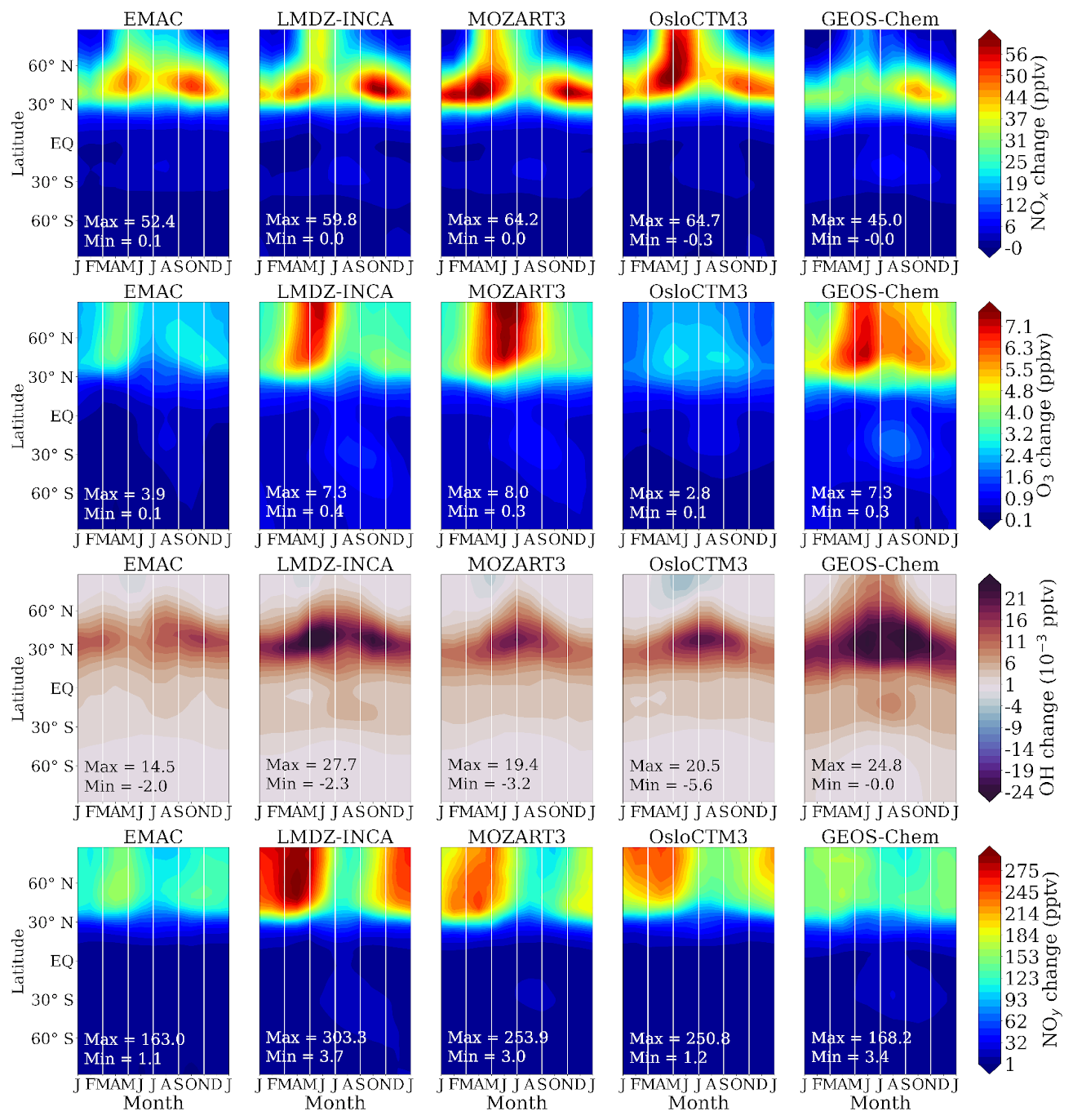
Figure 1 Hovmöller diagrams synthesizing the mean response of NO_x, O₃, OH and NO_y (from top to bottom), for the five models (from left to right). Each diagram consists of a vertical average between 150 and 350 hPa, the x and y axis displaying the months of the year and the latitude, respectively. Please note the diverging colorbar for OH, as there are both positive and negative responses.

3.1.2 Geographical distributions in the UTLS

Further details on the geographical distribution are available in Figs. 2 and 3, displaying the perturbations averaged between 150 and 350 hPa as in Fig. 1. We choose to display all the months that correspond to the minimum or maximum ozone perturbation for at least one model, as shown in Fig. 1 where the ozone response is minimized in January for every model and is maximized from April until June depending on the model. In the northern extratropics, the ozone perturbation is more important in April for EMAC-NO_x, in May for LMDZ-INCA, and in June for MOZART3, OsloCTM3, and GEOS-Chem. Consistently between the five models, Fig. 2 shows that the NO_x perturbation is located near the main emission zone above North America, Europe, and the North Atlantic corridor, with a similar spatial pattern expected from the use of a similar emission inventory, but with different magnitudes reflecting the intermodel variability in the chemical and physical background conditions. These three areas mainly contribute to the midlatitude maximum highlighted in Fig. 1. The NO_x perturbation propagates eastward through the westerlies and/or the subtropical jet. Figure 3 shows a more homogeneous ozone perturbation compared to NO_x, as expected for a secondary pollutant. We still notice a geographical maximum above midlatitude Eurasia, downwind from the main NO_x emission area. During May, the perturbation generally spreads northward to the pole. The magnitude is stronger in LMDZ-INCA, MOZART3, and GEOS-Chem (on average: ∼ 7, 8, and 7.5 ppb respectively) than in EMAC-NO_x (∼ 4 ppb) and OsloCTM3 (∼ 2.5 ppb) despite similar emission magnitudes, which is discussed later. In April and May, the magnitude and distribution are particularly similar between LMDZ-INCA and MOZART3 (with the same local maximum near the Eurasian subtropical jet in April), then the responses diverge in June when the magnitude keeps increasing for MOZART3 and decreases for LMDZ-INCA. The maximum response in OsloCTM3 is more localized and peaks around 30° N above the Atlantic.

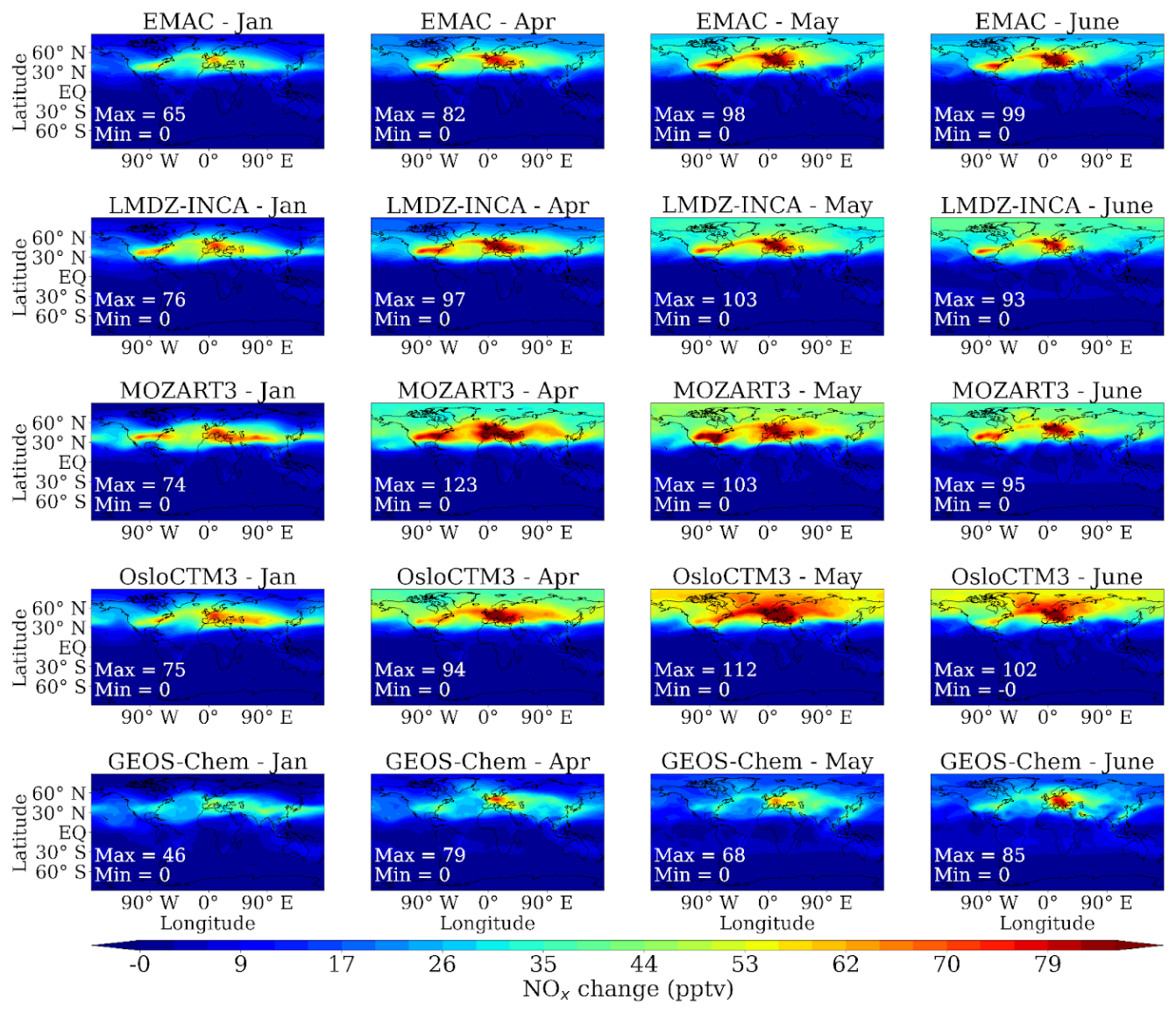
Figure 2 Mean geographical distribution of NO_x response to the aviation emissions averaged between 150 and 350 hPa, for January, April, May and June (from left to right), for the models EMAC-NO_x, LMDZ-INCA, MOZART3, OsloCTM3, and GEOS-Chem (from top to bottom). Geographical extrema are indicated in the bottom-left corner of each panel. The perturbation is rescaled with respect to global aircraft NO_x emissions for each model.

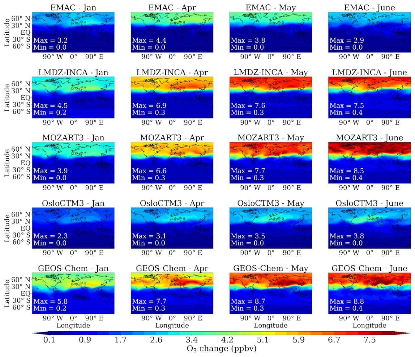
Figure 3 Same as Fig. 2 for ozone.

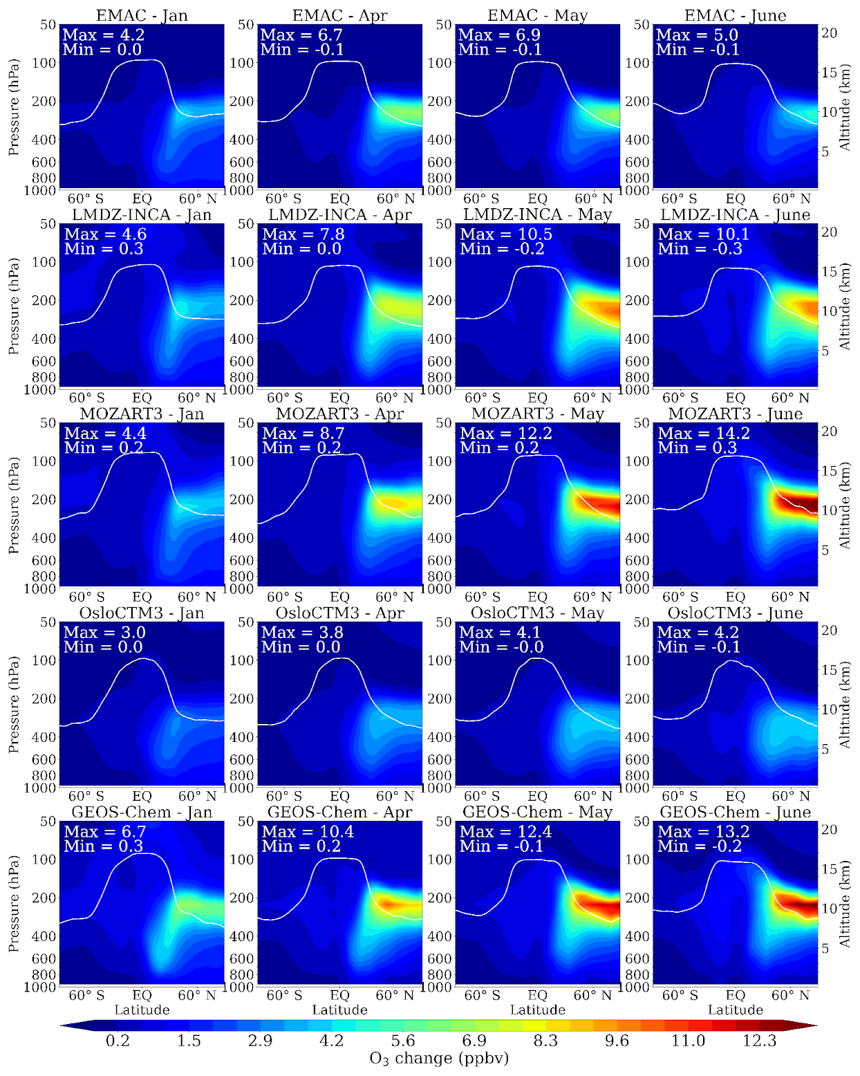
3.1.3 Zonal cross sections

Vertical information is provided in Figs. 4, 5, and 6, which display the mean zonal cross section for NO_x, ozone, and OH perturbations respectively. In every species, the main perturbation takes place near the climatological altitude of the model lapse-rate tropopause. In January, when the aviation-induced response is weakest, the perturbation is constrained around 40° N, while in spring and summer months, the response includes the higher latitudes. The perturbation even peaks north from 40° N for ozone, with the highest values generally in the lowermost stratosphere. An extension of the mean ozone perturbation is visible at low latitudes (as for NO_x, to a lesser extent), downward and equatorward, which can be linked to the aircraft trajectories and to subsidence motions.

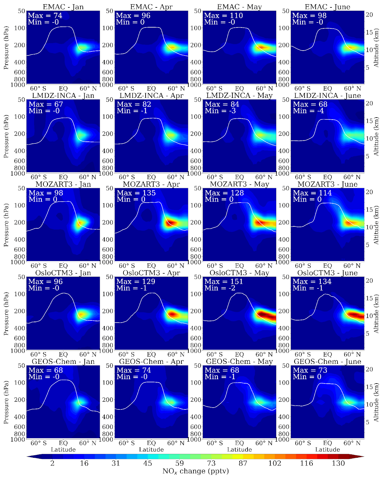
Figure 4 Mean zonal cross sections of NO_x response to the aviation emissions during January, April, May, and June (from left to right), for each model (from top to bottom). The white line represents the position of the climatological thermal tropopause. The extremes are indicated in the top-left corner of each panel. The perturbation is rescaled with respect to global aircraft NO_x emissions for each model.

Some differences are well visible between the models. Contrasting with the ozone perturbation generally in the altitude range of 8–12 km, the OsloCTM3 ozone response is located lower in the troposphere, in the range ∼ 5–10 km. In June, these lower altitudes in ozone perturbation are characterized by the strongest NO_x perturbation in the LMS, with a zonal mean above 120 ppt at all latitudes beyond 45° N. By contrast, the other models do not reach 100 ppt (LMDZ-INCA, GEOS-Chem), or very locally (EMAC-NO_x, MOZART3). In terms of mixing ratio, the maximum value of the ozone response ranges between 3.0 and 6.7 ppb in January, with three models relatively similar to each other (EMAC-NO_x, LMDZ-INCA, and MOZART3, within a range of 4.2–4.6 ppb). During the seasonal peak, the maximum value exhibits more discrepancies, with two models having lower maxima (4.1 and 6.9 ppb for OsloCTM3 and EMAC-NO_x respectively), two models having higher maxima (14.2 and 13.2 ppb for MOZART3 and GEOS-Chem), and one model having intermediate values (10.5 ppb for LMDZ-INCA). A stronger summertime ozone perturbation with MOZART3 compared to EMAC-NO_x and OsloCTM3 has also been reported in Søvde et al. (2014), with REACT4C emissions for 2006. Compared to the zonal cross sections shown in Fig. 5, we can compare the ozone sensitivities between the two studies, after rescaling linearly the ozone perturbation in the former study to equalize the NO_x emissions with the CEDS emissions during 2014–2018. With MOZART3, the maximum ozone response during JJA remains similar between the two studies, and 16 % lesser in DJF in the current study. With EMAC-NO_x and OsloCTM3 however, still in the current study compared to Søvde et al. (2014), the maximum ozone response is substantially weaker in both seasons (−38 % and −47 % in summer, and −39 % and −51 % in winter). Also, in the current study, the GEOS-Chem winter and summer perturbations in ozone reach ∼ 7 ppb in DJF and ∼ 12 ppb in JJA, which compares well with Eastham et al. (2024).

Figure 5 Same as Fig. 4, but for ozone.

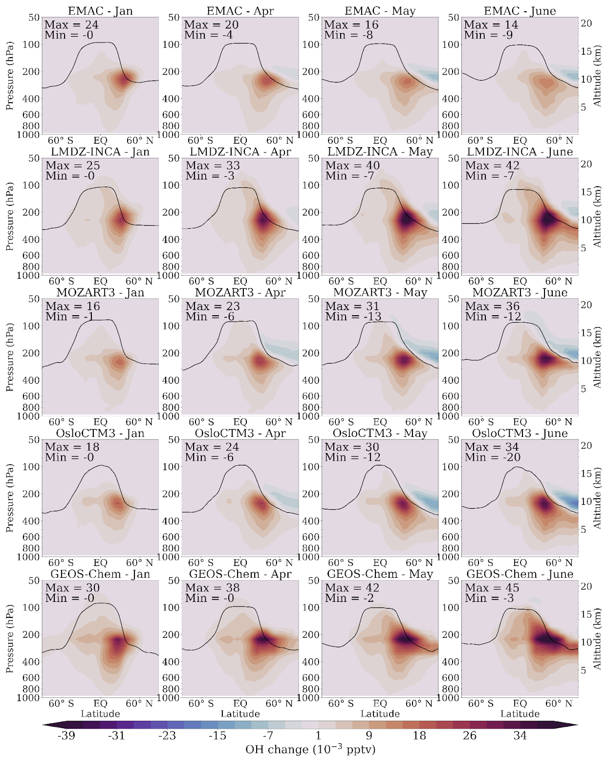
In Fig. 6, each model shows a positive wintertime OH response centered at 30° N and located mainly below the tropopause. In spring, the models generally exhibit a dipole structure with positive values centered near 40° N, mostly below the tropopause as well, and a negative response at high latitudes in the LMS (further discussion on chemical mechanisms responsible for the perturbation patterns is available below). The negative values are more pronounced with OsloCTM3, less pronounced with EMAC-NO_x, and insignificant with GEOS-Chem.

Figure 6 Same as Fig. 4, but for OH.

Concerning the studies that focus on the past decade (notably Søvde et al., 2014; Brasseur et al., 2016), one has to keep in mind that the ozone perturbation does not increase linearly with the NO_x emissions. This non-linearity can be explored with ancillary runs from three models (LMDZ-INCA, MOZART3, and OsloCTM3) based on the same protocol, using a new background run with 20 % less aviation NO_x emissions as described in Sect. 2.1. Table S2 indicates the ratio between the perturbation due to 100 % of aviation emissions and to the upper 20 % of aviation emissions, i.e. in the context of a poorer and a richer NO_x background, respectively. The ratio in the NO_x response varies from 0.92 (MOZART3) up to 1.04 (OsloCTM3), but the ratio for ozone is greater than 1 for all three models. It denotes a stronger sensitivity of about 10 %–20 % of O₃ to NO_x emissions with the lower NO_x background, which is consistent with a mostly NO_x-limited regime. As a consequence, Table S2 also shows that the aviation-induced decrease in methane lifetime is enhanced by a factor of 5 % for OsloCTM3 and 9 % for both LMDZ-INCA and MOZART3.

3.1.4 Involved chemical mechanisms

The causes for the spatial distribution of the ozone response have been investigated using the chemical production and loss terms for ozone from the models that provided them as diagnostic output, i.e. EMAC-NO_x and LMDZ-INCA. This paragraph sums up the characteristics shown by most species represented in this study to discuss the processes that might explain the ozone response. Figure S1 shows the ozone production term reaching its maximum in the midlatitude UT where the NO_x emissions are the most important, and extending northward in spring-summer, but only in the UT. It excludes local photochemical production as the source of the main O₃ perturbation in the LMS, and suggests two other factors to explain this pattern. First, the enhanced photochemical production in the UT tends to reduce the ozone vertical gradient (as background ozone is less abundant in the UT than above) and, subsequently, the LMS O₃ loss by cross-tropopause exchange through turbulent mixing. Second, although the chemical loss term (Fig. S2) increases in the mid-troposphere as ozone increases and water vapour remains relatively abundant (thus involving the reaction O(¹D) + H₂O → 2 OH), the chemical loss term decreases in the high-latitude LMS during spring–early summer. The spatial correlation with OH (Fig. 6) suggests that the ozone perturbation in the LMS is rather linked to lessened ozone destruction from the reaction O₃+ OH → HO₂+ O₂, despite the higher springtime ozone abundance due to the Brewer–Dobson circulation (e.g. Cohen et al., 2018). At these altitudes, stratospheric ozone destruction is essentially caused by the HO_x (= OH + HO₂) catalytic cycle (with a contribution of ∼ 80 % in June, see Brasseur and Solomon, 2005, Fig. 5.71, p. 416), involving the reactions:

$$\begin{array}{}\text{(R1)}& {\displaystyle }{\mathrm{O}}_{\mathrm{3}}+\mathrm{OH}\to {\mathrm{HO}}_{\mathrm{2}}+{\mathrm{O}}_{\mathrm{2}}\text{(R2)}& {\displaystyle }{\mathrm{O}}_{\mathrm{3}}+{\mathrm{HO}}_{\mathrm{2}}\to \mathrm{OH}+\mathrm{2}{\mathrm{O}}_{\mathrm{2}}.\end{array}$$

One can note that in the HO_x catalytic cycle, Reaction (R2) is specific to the lowermost stratosphere, as O(¹D) is too rare to make the reaction O(¹D) + HO₂→ OH + O₂ significant, contrary to the middle and upper stratosphere. Concerning the OH decrease in the LMS, we can relate it to the following reactions induced by the NO_x injection:

$$\begin{array}{}\text{(R3)}& {\displaystyle }\mathrm{NO}+{\mathrm{HO}}_{\mathrm{2}}\to {\mathrm{HNO}}_{\mathrm{3}}\text{(R4)}& {\displaystyle }{\mathrm{NO}}_{\mathrm{2}}+\mathrm{OH}\to {\mathrm{HNO}}_{\mathrm{3}}.\end{array}$$

These four reactions explain that aircraft NO_x neutralizes the main ozone sink in this region. It is illustrated by enhanced NO_x levels extending into the polar LMS during the same season, and with HNO₃ increasing substantially (shown in Fig. S5). As the primary pollutants emitted mainly in the midlatitudes have their response extending into the LMS in winter as well (BC in Fig. 8, next section; SO₂ in Fig. S4), the wintertime confinement of the NO_x response in the midlatitudes cannot be due to transport only, which suggests a particularly short NO_x chemical lifetime compared to the poleward transport duration. During spring – summer, however, part of HNO₃ is photolyzed back to NO_x, which can explain the northward extension of the NO_x response after the polar night.

3.1.5 Dependence on the chemical background

To explore the diversity in model responses to aviation NO_x emissions further, the scatterplots shown in Fig. 7 display the responses in ozone and OH versus the background concentrations of NO_x, CH₄, ozone, NO_y, and H₂O for each model. It appears that the responses in ozone and OH in the UTLS are generally stronger in models with lower NO_x (and lower NO_y) UTLS background, though this is not the only factor controlling O₃ and OH sensitivities to NO_x emissions. The OH response is correlated with the ozone response, and with the H₂O background if not for GEOS-Chem. It is higher with GEOS-Chem notably because this model specifically does not show an OH negative response in the polar LMS. One possible explanation comes from the spatial distribution in NO_x emissions that differs between Flightradar24 and CEDS inventories as mentioned in Sect. 2.2, leaving part of the emitted NO_x evolving in different chemical regimes between GEOS-Chem and the other models. On the opposite, the OH response is lower with EMAC-NO_x as both the ozone response and the H₂O background are relatively low. The OH response is comparable between MOZART3 and OsloCTM3, because of their strong negative response in the LMS, as seen in Fig. 6. The net OH response is higher with LMDZ-INCA (as expected from Fig. 6), characterized by a stronger positive response in the mid-latitudes and a weaker negative response in the high-latitude LMS. This positive OH response is consistent with the H₂O tropospheric background being the greatest in LMDZ-INCA, though the hydroperoxyl radical (HO₂) is another source of OH in the UT, which we did not investigate here. Last, we do not see any clear signal linking the perturbations to the background in methane or ozone, at least with our method, as the interpretation of these scatterplots remains limited. Concerning EMAC-NO_x, we notice that, as indicated in the companion paper (Cohen et al., 2025), the UTLS is the driest compared to the other models, though the LMS is the moistest. As done in Cohen et al. (2025), treating the UT and LMS separately with a daily resolution could highlight some links between these chemical species.

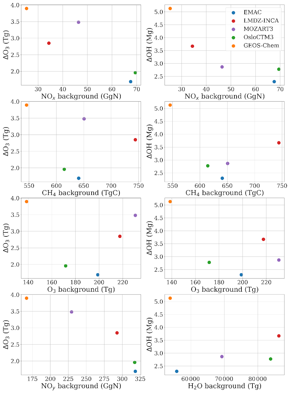
Figure 7 Perturbations in O₃ and OH mass burdens between 150 and 350 hPa (y axis) versus the backgrounds in NO_x, CH₄, O₃, and NO_y for ozone and H₂O for OH, between 150 and 300 hPa. The perturbations are normalized to the NO_x emissions. Each color represents a model, as indicated in the legend in the top right panel.

3.2 Aerosols

Four models investigated the impact of aircraft emissions on aerosols. The LMDZ-INCA and OsloCTM3 models share the common protocol, GEOS-Chem follows a similar set-up (Quadros et al., 2025), while the EMAC-aer model is represented by the output from Righi et al. (2023) with a substantially different simulation set-up (see Sect. 2.2). The contribution of aviation to atmospheric aerosols is shown in Figs. 8–10. It is shown for the same months as for gaseous species for consistency, though it is not optimal for every species. It is worth reminding that the EMAC-aer model is more accurate (as it is equipped with a detailed two-moment aerosol microphysical scheme) than the other models (characterized by simpler aerosol representations). Also, the EMAC-aer model is not used with a QCTM mode, hence the existence of negative values in BC and SO₄ due to changes in dynamics and physical processes. For these two species, the models generally show a maximum in the UTLS as for NO_x, in terms of zonal cross sections. OsloCTM3 has a much weaker response in the UTLS. For BC, all the models exhibit a local maximum at the mid-latitude surface, due to the take-off and landing phases (in Northeast America, Europe, and East Asia), and possibly to subsidence. The LMDZ-INCA and GEOS-Chem models show similar responses, with a maximum in April. All the models except OsloCTM3 show a summertime minimum for BC. The sulfate perturbation reaches its maximum at high latitudes in May with LMDZ-INCA and EMAC-aer, and in July with GEOS-Chem (shown in Fig. S7). The SO₄ seasonality is similar to the ozone seasonality, as photochemistry increases and promotes further the conversion of sulfur dioxide (SO₂) into SO₄, thus enhancing the formation of sulfate aerosol, as explained in Terrenoire et al. (2022) and Prashanth et al. (2022). For both BC and SO₄, the EMAC-aer model has a much stronger response, in the UTLS but also in the whole free troposphere. In this model, the maximum shifts from the lower free troposphere in winter up to the UTLS in summer. Most differences between EMAC-aer and the other models are consistent as EMAC-aer is the only model including the Aitken mode in the aerosol size distribution of aircraft emissions, and with an important proportion (91 % of emitted soot, and of primary sulfate particles, as supported by observations: Petzold et al., 1999; Mahnke et al., 2024), except the sulfate maximum in GEOS-Chem (July) that reaches higher levels than EMAC-aer.

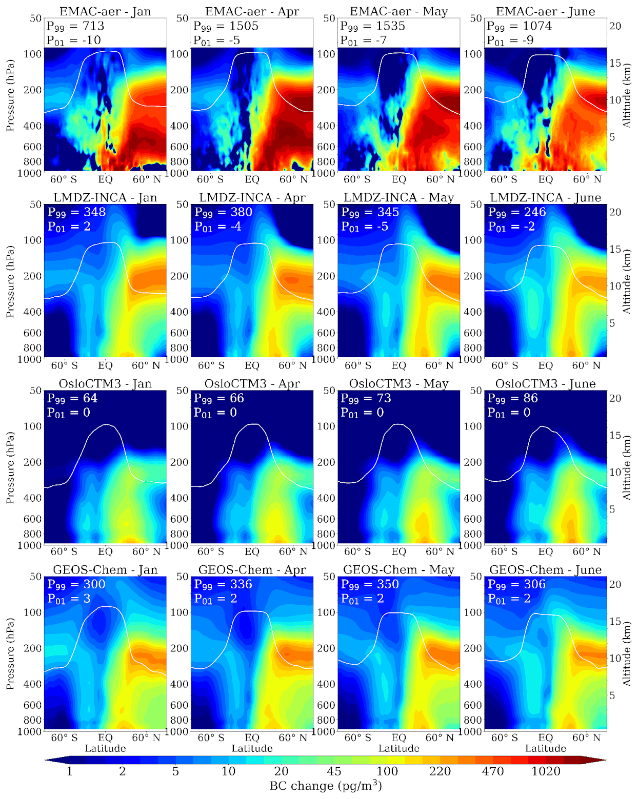
Figure 8 Mean zonal cross sections of the BC response to the aviation emissions during the months minimizing (left column) and maximizing the ozone response (right columns), for each model (from top to bottom: EMAC-aer, LMDZ-INCA, OsloCTM3, and GEOS-Chem). The white line represents the climatological position of the thermal tropopause (WMO, 1957). The percentiles 1 and 99 are indicated in the top-left corner of each panel. Please note the logarithmic scale in the color bar.

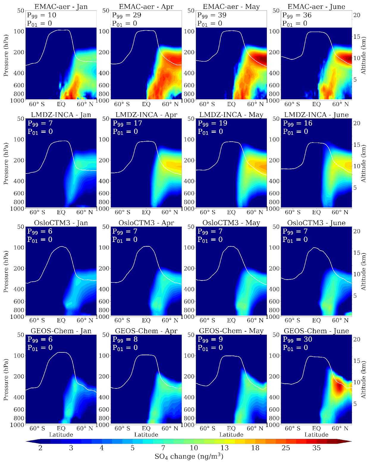
Figure 9 Same as Fig. 8, but for aerosol sulfate. Please note the logarithmic scale in the color bar.

Figure 10 Same as Fig. 8, but for aerosol nitrate.

The model diversity in aviation-induced aerosol abundances can be caused by a number of factors, such as the BC lifetime. The global mean BC lifetime we calculate in this study (Table S1) is comparable between EMAC-aer (7.7 d) and LMDZ-INCA (8.0 d). It is shorter in GEOS-Chem (5.1 d), and in OsloCTM3 (4.6 d), closer to the estimation of 5.5 d proposed in Lund et al. (2018b) to minimize the bias in BC concentration in the Arctic, though it remains a first-order metric which does not account for the important regional disparities, or the emission source. In the UTLS specifically, OsloCTM3 has the lowest background in BC, and also ammonia and SO₂ (Table S1), which tends to decrease further the SO₄ and NO₃ responses with this model. As OsloCTM3 performs well in reproducing CO and water vapour in the UT against IAGOS measurements (Cohen et al., 2025) while the other models are generally biased low, transport from the surface is unlikely to explain this discrepancy. It is rather linked to a stronger scavenging at high latitudes (Lund et al., 2018a). The global BC background in the UTLS shown in Table S1 is one order of magnitude higher with LMDZ-INCA, with 38 Gg compared to 1.54–3.95 Gg, whereas the BC response is similar between LMDZ-INCA and GEOS-Chem, and lesser than EMAC-aer. This discrepancy between LMDZ-INCA and the other models in the UTLS burden might be due to different parameterizations regarding convection and precipitation for BC emitted at the surface, as well as different representations of the BC solubility and size distribution, that control the BC transport up to the upper troposphere and deposition. The total burden is however similar between EMAC-aer (0.166 Tg) and LMDZ-INCA (0.169 Tg), hence their comparable BC lifetimes. It is characterized by a stronger burden in the UTLS and in the stratosphere for LMDZ-INCA compensated by a stronger burden in the lower troposphere for EMAC-aer. Compared to observations from aircraft campaigns, most models participating to the AEROCOM intercomparison project overestimate BC mass mixing ratios in the UTLS (Koch et al., 2009; Schwarz et al., 2013). Schwarz et al. (2013) notably showed an overestimation by a factor 6–20 above 300 hPa, in global average, for the models participating to the second phase of AEROCOM. Kaiser et al. (2019) concluded that EMAC with MADE3 (here EMAC-aer) was closer to the observations in the UT than the AEROCOM II model average, though the ultrafine particle number concentration tends to be overestimated at these altitudes.

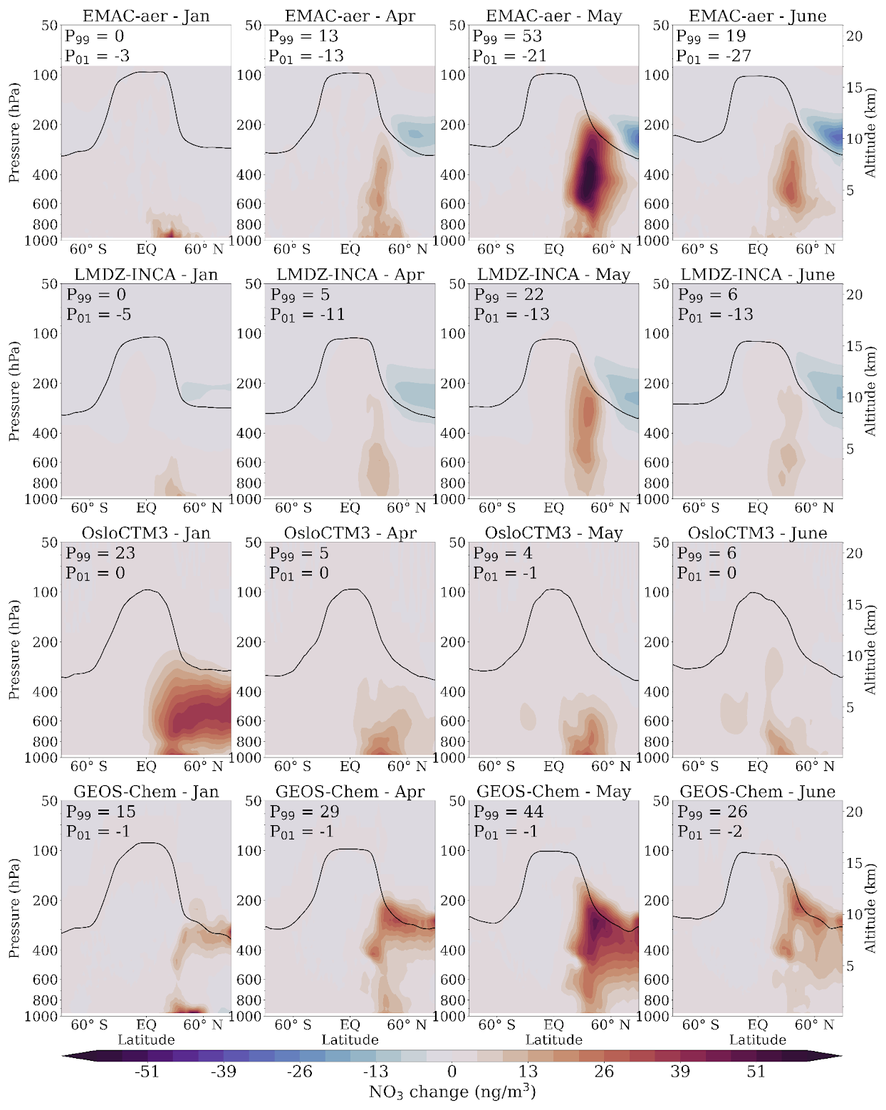
For NO₃, three models (LMDZ-INCA, GEOS-Chem, and EMAC-aer) show a positive response with a vertical shape in the midlatitude, along the whole tropospheric column, and with a peak in May, in the free troposphere. OsloCTM3 also exhibits a positive NO₃ perturbation at the same latitudes, but only in the lowermost troposphere, and with a vertically broad peak in January, centered on the middle troposphere. For LMDZ-INCA and EMAC-aer, the perturbation is characterized by a dipolar structure, with negative values in the high-latitude lowermost stratosphere. According to the explanation provided by Terrenoire et al. (2022) and Righi et al. (2023), both sulfate and nitrate combine with the background gaseous ammonia to form aerosol, respectively via the formation of ammonium sulfate and ammonium nitrate. Given that NH₃ is limited in the UTLS, and that SO₄ reacts faster with ammonia than NO₃, the ammonium sulfate formation in this region results in a decrease in ammonium nitrate aerosols. On the contrary, in the lower troposphere, ammonia is abundant such that the SO₄ perturbation is not sufficient to compete with NO₃ in the aerosol formation.

In the literature, studies including aerosol perturbations from aviation are fewer than for the gas phase. Among the studies using different models than this paper, Unger et al. (2013) present the same spatial pattern in annual means (in their Fig. S2a), with a SO₄ perturbation maximum in the UTLS and visible effects from subsidence, and a dipole in the NO₃ perturbation. Once rescaled up to 2014–2018, the values are higher than most of our models, with a cruise maximum between 14 and 28 ng m⁻³ for SO₄ (6, 11, 13, and 23 ng m⁻³ in our study) and between 70 and 140 ng m⁻³ (−70 and −140 ng m⁻³) for NO₃ in the extratropical UT (in the high-latitude LMS). Concerning sulfur, Kapadia et al. (2016) uses the TOMCAT CTM and shows that the impact of sulfur content in aircraft fuel increases SO₄ in the high-latitude UTLS up to 6–7 ng m⁻³ averaged over the year 2000, which would correspond to 7.9–9.2 ng m⁻³ once rescaled up to the NO_x emissions used in our study. It is comparable to our intermodel range, in the lower part, but does not include the SO₄ produced from non-aviation SO₂.

It is worth mentioning the aviation impact on surface concentrations as represented by these models, shown in Figs. S11–S13. The surface is represented by the lowermost level (up to ∼ 60, 70, 20, and 130 m for EMAC-aer, LMDZ-INCA, OsloCTM3, and GEOS-Chem respectively). As in Righi et al. (2023), we performed a t-test on EMAC-aer output in order to assess the significance of the perturbation against the interannual variability. We choose to show only the gridcells where the perturbation is characterized by a p-value lesser than 0.05, consistently with Righi et al. (2023). On average in the period of interest, the BC seasonal maxima at the surface are located at the eastern and western coasts of the US, in Europe, and, to a lesser extent, in East Asia (Fig. S11). These maxima are generally at ∼ 1 ng m⁻³ except for EMAC-aer, which maxima reach ∼ 4 ng m⁻³ in the eastern US, Europe and around the Mediterranean basin. The increase in the other two aerosol compounds is more significant by mass. SO₄ perturbation takes place in western Europe, US, and the subsidence regions as North Africa–Middle East with a summertime average of ∼ 35–45 ng m⁻³ (70–90 ng m⁻³ for EMAC-aer). For NO₃, the impact is generally stronger in winter in North America, western Europe, South Asia, and East Asia. The latter reaches wintertime NO₃ perturbations of 100–460 ng m⁻³. As for the UTLS, the differences between EMAC-aer and the other models are large, which suggests an important sensitivity of both climate and air quality impacts to the size of emitted aerosols (as discussed in Gettelman and Chen, 2013; Righi et al., 2013), and highlights the need for another model intercomparison with a more accurate aerosol parameterization in the model ensemble.

4 Radiative impact of aviation emissions

Finally, we show the estimated radiative impact of the atmospheric composition responses described in Sect. 3. The sensitivity of the radiative forcing to mixing ratio responses at different altitudes and locations is heterogeneous for both ozone and aerosols, for example with the highest RF per DU response for ozone in the tropical upper troposphere (Skeie et al., 2020, Fig. S1). Figure 11 shows the global annual average vertical profiles of the aerosol (aerosol-radiation interaction only) and ozone instantaneous RFs (i.e. without ERF scaling). This provides additional information about how the responses in concentration (e.g. Fig. 1) relate to the resulting radiative forcing. For ozone, the models show a similar vertical profile, but with different magnitudes and small variations in the altitude of the peak ozone response (Fig. 11f). The high RF sensitivity to ozone response in the upper troposphere (compared to the lowermost stratosphere) means that although the magnitude of ozone concentration response in OsloCTM3 is lower than in EMAC-NO_x (Fig. 5), the resulting RF is larger for OsloCTM3 since the response occurs in a more sensitive region. Similarly, while the peak (June) ozone concentration responses are similar in GEOS-Chem and MOZART, GEOS-Chem exhibits a stronger response to aviation emissions in most other months (Fig. 1) resulting in a substantially stronger ozone forcing in the peak ozone response region.

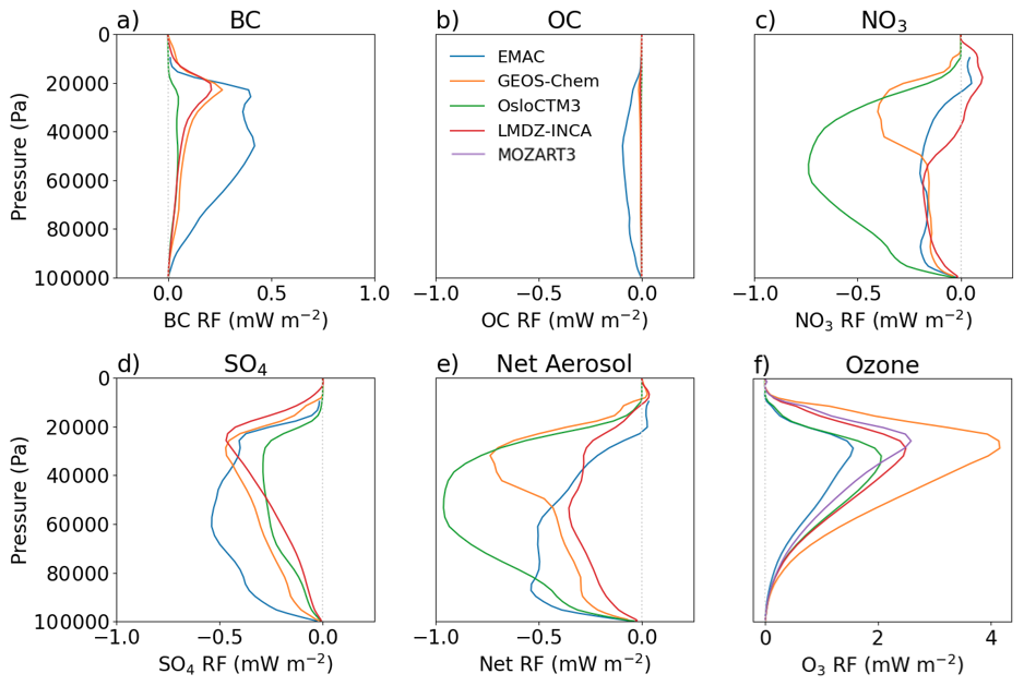
Figure 11 Vertical distributions of global annual average radiative forcing from aviation emissions from aerosols (aerosol-radiation interaction only) and short-term ozone response. (a) black carbon, (b) organic carbon (c) nitrate, (d) sulfate, (e) net aerosol and (f) short-term ozone. Each color corresponds to a model. EMAC-aer is represented in panels (a)–(e) and EMAC-NO_x in panel (f).

For aerosols, there are substantial differences not only in magnitude but also in the relative role of individual aerosol species across the models, as seen in the vertical profiles in Fig. 11a–e. These largely follow the model differences in underlying aerosol concentrations, with large SO₄ responses in EMAC-aer and NO₃ responses in OsloCTM3. The net NO₃ responses in EMAC-aer and LMDZ-INCA are smaller, likely due to a negative response in the high-latitude lowermost stratosphere that compensates part of the NO₃ production. While the spread in ozone RF mainly arises from differences in the UTLS region, there are important contributions to aerosol forcing and thus model diversity extending through the troposphere, particularly for SO₄ and NO₃. The RFs shown in Fig. 11 and discussed in this section are converted to ERFs to enable comparison with other studies in the following paragraphs (see Sect. 2.3). It is worth noting that in our modelling set-up, the nitrate particles forcing is not only related to aircraft NO_x emissions driving the formation of ammonium-nitrate particles (NH₄NO₃). It is also affected by the oxidation of sulfur dioxide (SO₂) into sulfate particles due to NO_x-induced OH formation. This additional sulfate then collides with ammonia to form ammonium-sulfate particles ((NH₄)₂SO₄), thus competing with nitric acid to react with ammonia, and thus to form nitrate aerosol. Terrenoire et al. (2022) show that the nitrate forcing is more negative (or less positive) when one accounts for the aircraft NO_x effect on aerosols. With this limitation in mind, we note that the nitrate forcing reduces the net NO_x forcing from a model mean of 18.3 to 11.9 mW m⁻².

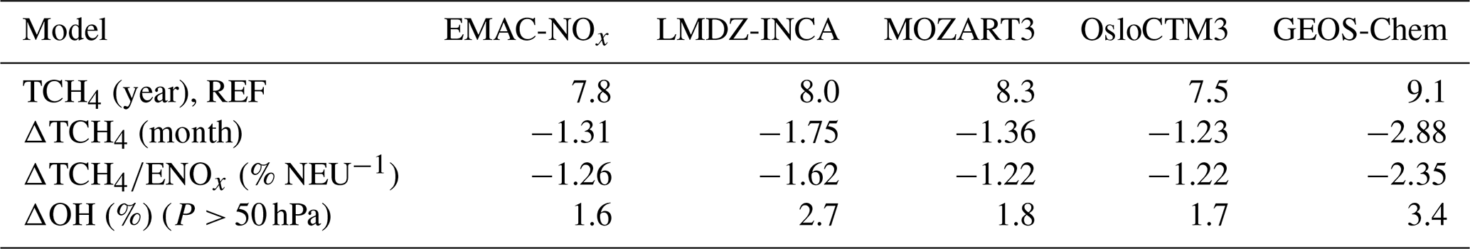
We estimate a global mean aviation NO_x-induced ozone ERF between 28 and 56 mW m⁻² (Fig. 12a, Table S3). GEOS-Chem shows the strongest response, while EMAC-NO_x shows the weakest, which is consistent with the ozone concentration responses shown in Figs. 1 and 5. Figure 12a also shows the global mean net NO_x ERF due to the longer-term decreases in CH₄, ozone, and stratospheric H₂O. The relative response of these forcers between models is similar to that for short-term ozone, with the strongest ERF found for GEOS-Chem, although OsloCTM3, EMAC-NO_x, and MOZART3 simulate more similar long-term net NO_x ERFs than for the short-term ozone. The estimated ERF due to aviation NO_x-induced changes in CH₄ ranges from −34 to −18 mW m⁻². The spread reflects differences in the modeled methane lifetime and mean OH concentration (Table 5). The results from EMAC-NO_x, MOZART3, and OsloCTM3 are close to each other, with a range of −1.22 % to −1.26 % NEU⁻¹ in methane lifetime. The sensitivity is ∼ 30 % higher with LMDZ-INCA, both because of a substantially greater background in CH₄ (744 TgC compared to 614–651 TgC from these three models, see Table S1) and a stronger OH sensitivity (see Fig. 7). The GEOS-Chem sensitivity is ∼ 90 % greater, with a lower methane background outweighed by more OH production.

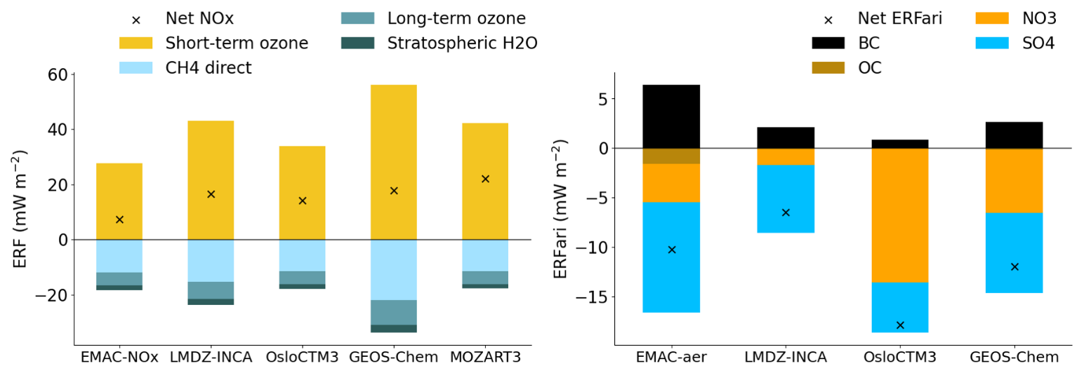
Figure 12 Global mean ERF from aviation emissions in the present day for (a) net NO_x emissions, comprising short and long-term ozone, methane and stratospheric water vapour, and (b) aerosol-radiation interactions (ERF_ari), comprising contributions from BC, OC, NO₃ and SO₄.

Table 5 Background values and perturbations (both absolute and normalized to the aviation NO_x emissions) in the tropospheric methane lifetime (TCH₄) and the OH concentration. As a reminder, we define the NO_x-emission unit as 1 NEU = 1 TgN yr⁻¹.

Overall, we estimate a positive net aviation NO_x ERF in these model experiments, with a multi-model mean value of 18.3 mW m⁻² and a range from 9.4 to 24.5 mW m⁻². The strongest ERF is estimated by MOZART3, despite the individual ozone and CH₄ contributions being strongest in GEOS-Chem, due to these effects partially cancelling each other. EMAC-NO_x simulates the weakest net NO_x ERF, followed by OsloCTM3 and LMDZ-INCA.

Myhre et al. (2011) calculated a net NO_x ERF of +6 ± 5 mW m⁻² in the AIR experiment (100 % reduction of year 2000 aviation, four models), compared to our estimate of 18.3 [9.4; 24.5] mW m⁻². Terrenoire et al. (2022) calculated an ERF of 14.8 mW m⁻² for 2018 total aviation fuel with the LMDZ-INCA model. Lee et al. (2021) derived an estimate of 17.5 mW m⁻² (90 % likelihood range [0.6, 29] mW m⁻²) from Lee et al. (2021) based on 18 models from 20 studies, normalized to 2018 levels. When normalized to account for differences in NO_x emissions, the corresponding values from Myhre et al. (2011), Terrenoire et al. (2022), and Lee et al. (2021) are 8 ± 7, 11.6, and 13.7 [0.5, 23] mW m⁻², respectively. The modeled range of net NO_x ERF in this study is smaller than found by Myhre et al. (2011) and Lee et al. (2021), indicating that our five models may not represent the full spread of model diversity, though implementing a common protocol contributes to the reduction of this variability by eliminating some degrees of freedom. Also, normalizing with respect to the NO_x emissions does not account for nonlinearities in the NO_x ERF, which might be significant between two years with substantially different emissions (e.g. 2018 vs. 2000).

Figure 12b shows the global mean component and net RF from aerosol-radiation interactions in the four models that provide aerosol information (with values provided in Table S4). We estimate a multi-model mean ERF from aerosol-radiation interactions (ERF_ari) of 2.9, −0.4, −7.8, and −6.3 mW m⁻² for BC, OC, SO₄ and NO₃, respectively. The mean net ERF_ari from these simulations is −11.6 mW m⁻², with large model diversity in magnitude and dominant aerosol species, as shown in Fig. 11. Lee et al. (2021) gave a best estimate of aviation BC ERF_ari of 0.94 mW m⁻², with a 90 % likelihood range of 0.1–4.0 for 2018 emissions. This is close to our weakest estimate of 0.82 mW m⁻² (OsloCTM3), with our multi-model mean within their range. Our estimated SO₄ ERF_ari is close to the best estimate of −7.4 mW m⁻² from Lee et al. (2021). Fewer studies have considered the effect of aviation nitrate. With a similar set-up as in the current work, Prashanth et al. (2022) calculated a net RF of −0.67 mW m⁻² with GEOS-Chem, and Terrenoire et al. (2022) a net RF of 0.14 mW m⁻² with LMDZ-INCA. Among the two studies mentioned in Brasseur et al. (2016) regarding NO₃ RF in 2006 (that we rescale up to 2014–2018), Unger et al. (2013) calculate a net RF of −4.0 ± 1 mW m⁻² (−5.5 ± 1.4 mW m⁻²) with the GISS-E2 model, and the IGSM model calculated a net RF of −7.5 mW m⁻² (−10.3 mW m⁻²). This low number of estimations and their high variability highlight the need for additional modelling experiments, with the most recent model versions, and with a constraining protocol for the simulation setup.

We note that these are not complete estimates of aerosol radiative forcing: aerosol-cloud interactions are not included here. Aerosol-cloud ERF currently has no best estimate due to high uncertainty in the underlying process representation in the models. For the impact of aircraft particles on low-level clouds, Righi et al. (2013) found an RF range from −70 to −15 mW m⁻², depending on the assumptions on the size of the particles. A similar dependency was also found by Gettelman and Chen (2013) who reported a range from −164 to −23 mW m⁻². This effect also depends on sulfur emission altitudes (Kapadia et al., 2016; Matthes et al., 2021). For soot-cloud interactions, uncertainties are even larger, with a wide range of values reported by different studies, with disagreement both in magnitude and sign, including several studies reporting a statistically non-significant effect (see Righi et al., 2021 and references therein). This depends on the models used, with different representation of the ice formation process and different assumptions on the ice-nucleating properties of aviation soot. In a very recent model study supported by laboratory measurements on the ice-nucleating properties of aviation soot, Righi et al. (2025) found a non-statistically significant ERF for aviation soot-cloud interactions. Lastly, the other major component of the ERF from aviation emissions here is contrail cirrus formation, which could not be simulated within the current capability of the models used in this study. Lee et al. (2021) estimated the contrail cirrus ERF as 57.4 [17, 98] mW m⁻².

5 Summary and conclusion

In light of increasing air traffic, we perform and document a new multi-model assessment of the atmospheric composition response to aviation NO_x and aerosol/aerosol precursors emissions, and the associated radiative forcing of climate, notably providing the first model intercomparison on the impact of aviation on nitrate aerosol. The purpose is to refine estimates of the impact of aviation by limiting differences between the models in their implementations, for a better understanding of the intermodel variability in the results. We present a model intercomparison involving five state-of-the-art chemistry-transport models (CTM) or chemistry-climate models (CCM). For this study, each participating model provides a set of present-day runs, including at least one reference run with all the anthropogenic emissions, and one perturbation run without aviation emissions. The models use the same anthropogenic and biomass-burning emission inventories, and most of them use the same aircraft emissions. The models used to estimate the impact of aviation-induced aerosols are also applied to the gaseous phase, thus maximizing the consistency between the estimates for gaseous and aerosol species. For all models, the effective radiative forcings are calculated with the same radiative code, the same grid, and the same feedback factors.

Several similarities between the models are encouraging regarding our understanding of the chemical sensitivity to aircraft emissions. For both gaseous and aerosol species, the main perturbation generally occurs at flight cruise altitude, in the extratropical UTLS, around 10 km above sea level. For gaseous species, the NO_x and ozone responses show a good agreement across the models in terms of both seasonal and spatial patterns. Seasonally, the models show lower values in January and higher values in spring–early summer, though the latter can take place in April, May, or June, depending on the model. Geographically, all the models present a NO_x response maximum (85–112 ppt) near the area of highest flight density (Europe, North Atlantic corridor, and eastern US, all of them in the mid-latitudes), and a moderate perturbation (> 40 ppt) confined to the northern mid-latitudes in winter, and expanding horizontally into the polar LMS in spring–early summer. Across the models, an ozone response maximum is consistently simulated following the NO_x perturbation (2.3–5.8 ppb in January, 3.8–8.8 ppb in April–June), although the mechanism linking NO_x to ozone differs between the upper troposphere and the lowermost stratosphere. For each TgN of emitted NO_x throughout the year, the response of global ozone burden ranges between 5.6 and 10.0 Tg, and the methane lifetime perturbation ranges between −1.2 and −2.9 months (−1.75 month without the most sensitive model). Our results suggest that the different background composition at cruise altitudes across the models, notably in NO_x and humidity, is a relevant factor for explaining the different magnitudes of the model responses in OH concentration and methane lifetime. Based on these experiments, we estimate a multi-model mean net aviation NO_x ERF of 18.3 mW m⁻², with a range from 9.4 to 24.5 mW m⁻². Using the same protocol applied to the models, our estimate and range of net NO_x ERF, along the relative contribution from ozone, methane, and water vapor changes, are consistent with previous studies when normalized to present-day emissions. Thus, despite several studies and model development, robust assessment of the effects of aviation NO_x emissions remains challenging and in need of novel strategies. The multimodel approach remains particularly important as the model assessment in Cohen et al. (2025) emphasizes that no single model shows best skill in all the species and regions.

Aerosol species show a larger variability across models than is the case of gaseous species, in terms of global burden responses and distributions. It can be explained with the significantly larger spread in model complexity compared to the NO_x experiments, as most of the models are characterized by a relatively simple aerosol scheme. The contribution from aviation emissions to black carbon (BC) differs by up to a factor 8 across the models, and sulfate (SO₄) varies by up to a factor of 2. The combined radiative effects from these two species remain similar across the models, each species compensating for the difference of the other one. Last, nitrate (NO₃) varies substantially with a factor of 14 between the most and the least sensitive models (reduced to a factor ∼ 2 if excluding the model with the strongest response to aviation emissions). While the spatial patterns of BC and SO₄ tend to be similar across models, with a noticeable impact on the UTLS (except one model), the NO₃ patterns can differ radically across the models and, notably, only two of four models simulate a negative perturbation in the polar LMS. A noticeable impact is identified on surface concentrations for SO₄ and NO₃ for all the models, at least during one season. The net aerosol ERF_ari varies between −6.5 and −17.8 mW m⁻² (multi-model mean of −11.6 mW m⁻²), with the formation of sulfate and nitrate particles that reduces the net NO_x forcing by 43 % and 35 %, respectively. However, we also note that there is a factor 8 difference between the highest and lowest NO₃ forcings estimated. Moreover, relatively few studies have so far explored the role of aviation nitrate aerosols. While the direct effects of aerosols from aviation is sometimes argued to be small, our multi-model mean estimate of aerosol forcing is close to but of opposite sign to the net NO_x ERF. Further work to increase the amount of data and improve the understanding of the spread in simulated aerosol distributions is needed to constrain knowledge of the contribution from aerosols to the climate effect of aviation.

The discrepancies shown in this study highlight the need for a better understanding of gaseous components involving NO_y partitioning as it differs substantially through the models (Cohen et al., 2025), crucial to understand the role of oxidized nitrogen in atmospheric chemistry and climate (Wei et al., 2025). It also highlights the need for further modeling experiments on the aerosol parameterization as scavenging (depending on solubility and precipitation), their size distribution, the mixing state, and heterogeneous chemistry that also involves scavenging, as nitric acid (HNO₃) is a soluble precursor of nitrate aerosol. Further observations are needed for an assessment of the background aerosol properties. Understanding and reducing spread in modeled atmospheric concentrations is also a key step in constraining estimates of the present-day aviation-induced climate effects. This is increasingly important as proposed mitigation measures for the sector, such as alternative fuels, will affect not only CO₂ but also non-CO₂ emissions. Understanding the current impact is critical for assessing the net effect of future mitigation. Last, the future responses following several scenarios, along with sensitivity to the background chemical composition, will be investigated in a companion paper (Staniaszek et al., 2025).