Machine learning reveals strong grid-scale dependence in the satellite N_d–LWP relationship

The relationship between cloud droplet number concentration (N_d) and liquid water path (LWP) is highly uncertain yet crucial for determining the impact of aerosol-cloud interactions (ACI) on Earth's radiation budget. The N_d-LWP relationship is examined using a machine learning (ML) random forest model applied to five years of satellite data at grid resolutions ranging from 10° to 0.05° in 12 distinct regions. In the subtropics, the shape of the N_d-LWP relationship switches from an inverted-V at 1° grid-resolution to an “M” shape at 0.1° resolution with decreased $\frac{\mathrm{d}\ln \text{LWP}}{\mathrm{d}\ln N_{\mathrm{d}}}$ sensitivity. Tropical and midlatitude regions generally show a more positive sensitivity. Cloud sampling and filtering also influence this slope, wherein the exclusion of thin clouds, as commonly performed to reduce retrieval uncertainty, leads to strongly negative sensitivity across all regions. Precipitation is primarily responsible for driving the strength of the sensitivity, with strong positive slopes in raining clouds and negative and/or neutral responses found in non-raining clouds. A new method to compute radiative forcing from the ML model shows a robust Twomey radiative forcing across all regions and grid resolutions. However, LWP and cloud fraction adjustments to the radiative forcing, which are ∼50 % or smaller than the Twomey effect, decrease to negligible values with higher spatial resolution data. As Earth system models move toward higher spatial resolutions in the future, evaluating the LWP and CF adjustment contributions to the radiative forcing budget at these finer resolutions will be essential for evaluation and model development.

1 Introduction

Clouds are highly reflective and significantly cool the Earth, helping to keep the planet habitable. The more abundant they are, and the more water they contain, the greater the amount of solar radiation they reflect (Stephens, 1978). Increased aerosol concentrations can elevate planetary albedo by enhancing cloud reflectance through an increase in cloud droplet number concentration (N_d), cloud liquid water path (LWP), and cloud fraction (CF). However, if LWP and CF decrease as aerosol loading increases, more sunlight will be absorbed by the Earth, leading to a warming radiative effect. While the effective radiative forcing from aerosol-cloud interactions (ACI) (ERF_aci; Gryspeerdt et al., 2019) has a net cooling effect globally, estimates remain highly uncertain (Bellouin et al., 2020) due to limited understanding, large retrieval uncertainties, and challenges quantifying and attributing causality from the non-linear relationship between N_d and LWP.

The N_d–LWP relationship is non-linear and typically appears as an inverted-V shape when displayed as a column-normalized 2D histogram representing the conditional distribution P(LWP|N_d) (Gryspeerdt et al., 2019). This shape manifests from a rise in LWP as N_d increases below a threshold of approximately 30 cm⁻³, followed by a decrease for higher N_d. Examples of this relationship can be seen in satellite observations (Gryspeerdt et al., 2019), large eddy simulations (LES; Hoffmann et al., 2020), and in the Energy Exascale Earth System Model (E3SM; Christensen et al., 2023). The prevailing hypothesis governing this relationship provides separate physical explanations for the behavior in both the high and low N_d regimes. The ascending branch (at low N_d) results from the suppression of precipitation caused by more, but smaller, cloud droplets allowing LWP to increase (Albrecht, 1989). In the descending branch, entrainment of dry air into non-raining clouds tends to decrease LWP (Ackerman et al., 2004) by increasing N_d further. Dry air entrainment affects both branches, but when the clouds are non-precipitating, the LWP is subject to larger decreases (Chen et al., 2014).

Although this relationship has been used to infer causality in ACI, several factors complicate a direct causal interpretation. Aerosol effects can make the link between aerosol concentration and N_d nonlinear due to processes such as precipitation suppression and evaporation-entrainment feedbacks (Albrecht, 1989; Ackerman et al., 2004). Satellite retrieval errors and sampling limitations – such as the exclusion of thin clouds due to uncertainties or biases introduced by retrieval inaccuracies – further affect analyses (Grosvenor et al., 2018). Feedbacks, including wet scavenging and entrainment, impact N_d retrievals, while meteorological confounders, such as dry air intrusion coinciding with elevated aerosol levels, can reduce cloud water paths; each of these factors are detailed further in (Gryspeerdt et al., 2019). Recent assessments show that the propagation of spatial variability and errors in satellite retrievals can lead to the misinterpretation of positive LWP adjustments as negative in subtropical clouds, thereby leading to an underestimate of ERF_aci (Arola et al., 2022). The extent to which this relationship is controlled by these or a combination of these factors and whether similar biases or drivers are applicable outside of the subtropics remains largely unknown.

Current understanding of the N_d–LWP relationship derived from satellite observations at global scales is largely based on coarse spatial resolution data (e.g., 4° × 4° or 1° × 1° grids). While Arola et al. (2022) examined finer spatial resolutions (0.25° × 0.25°) of the N_d–LWP relationship it was over a limited area of the North Pacific, leaving an open question as to whether the results hold outside of the subtropics and over larger spatial extents. General circulation models (GCMs) with regionally refined meshes, such as the Simple Cloud-Resolving E3SM Atmosphere Model (SCREAM), have started generating ACI statistics at increasingly finer resolutions, down to 3 km (Caldwell et al., 2021). This raises pertinent questions about how the statistics of ACI change with varying spatial-scale resolutions, and whether meteorological regimes influence the 2D histograms of the N_d-LWP relationship. We generated a series of collocated global datasets at progressively higher grid-scale spatial resolutions (10, 5, 1, 0.5, 0.1, and 0.05°) and applied a machine learning (ML) model to extract non-linear behavior in the N_d–LWP relationship. From these new datasets and tools, we are able to answer the following questions:

• How does the structure of the N_d–LWP relationship change as the spatial grid resolution increases to finer scales?

• How do subtropical, tropical, and midlatitude regions differ in their N_d–LWP relationships?

• How does satellite filtering and sampling clouds with different characteristics influence the N_d–LWP relationship?

• What are the primary meteorological drivers shaping the N_d–LWP relationship?

• What is the impact of changing spatial resolution on the estimated radiative effects of ACI?

In this study, we aim to address these questions by examining how grid-scale resolution, regional differences, and meteorological factors influence the N_d–LWP relationship, and by applying a random forest ML model to our data set to enhance our understanding and prediction of these complex interactions and changes in radiative forcing. The data sets are described in Sect. 2, methods involving statistical sampling and ML methods are described in Sect. 3, results are described in Sects. 4 and 5, with Sect. 5 highlighting the ML analysis and conclusions in Sect. 6.

2 Data

2.1 Satellite Observations

The MODIS Collection 6.1 cloud product is derived from the observations acquired from the Aqua satellite, which follows a polar orbit crossing the equator at approximately 01:30 p.m. local time. This product includes retrievals of cloud optical properties such as effective droplet radius (R_e) and optical thickness (τ_c) at multiple wavelengths (1.6, 2.1, and 3.7 µm) and cloud thermodynamic phase, as well as infrared retrievals of the cloud top temperature (CTT), pressure (CTP), and height (CTH) (Nakajima and King, 1990; Platnick et al., 2017). These products are retrieved at a nominal spatial resolution of 1 km at the surface at nadir. Due to oblique viewing angles and projection effects onto Earth's curved surface, MODIS pixel size increases from 1 km at nadir to nearly 4 km at the swath edges. MODIS data are provided as 1354 × 2030-pixel granules. This dataset includes three filters applied to the MODIS retrievals for liquid warm clouds:

1. All. Includes retrieved cloud properties where phase =2 (liquid) and CTT >268 K.

2. Q06. Includes all filters from the All composite plus τ_c>4 and R_e>4 µm. This filter is called “Q06” because it uses the same set of constraints as those used in Quaas et al. (2006).

3. G18. Includes all properties from the Q06 composite plus 5 km CF >0.9, solar zenith angle (θ_solar) <65°, satellite zenith angle (θ_satellite) <55°, and sunglint pixel index (SPI) <30°. This filter is called “G18 because it uses the same set of constraints as those used in Grosvenor et al. (2018).

Following the same approach (and terminology for the filter names) as Gryspeerdt et al. (2022), N_d is computed for each composite using the equation $N_{\mathrm{d}}=\mathit{\gamma }f\left(\text{CTT}\right){\mathit{\tau }}_{\mathrm{c}}^{\mathrm{1}/\mathrm{2}}{R}_{\mathrm{e}}^{-\mathrm{5}/\mathrm{2}}$, where γ is the adiabatic condensation growth rate taking a value of $\mathrm{1.37}\times {\mathrm{10}}^{-\mathrm{5}}{\mathrm{m}}^{-\mathrm{0.5}}$, and $f\left(\text{CTT}\right)=\mathrm{0.0192}T-\mathrm{4.293}$ is the temperature-dependent condensation rate determined from the CTT retrieval.

AMSR-E, onboard NASA's Aqua satellite, operates at multiple microwave frequencies, allowing it to retrieve cloud water path and surface precipitation rate. It has a swath width of about 1445 km with a footprint of approximately 13 km² at the surface. Version 2 of the AMSR-E AE_Ocean(Rain) product provides retrievals of columnar cloud and rain water path as well as surface precipitation over each footprint using the 36.5 GHz channel (Wentz and Meissner, 2004).

The CERES instrument measures top of atmosphere radiances in the shortwave (0.3–5 µm), window (8–12 µm), and total (0.3 to 200 µm) spectral channels, with a spatial resolution of approximately 20 km at nadir. Operating in cross-track, along-track, and rotating azimuth plane modes aboard the Aqua satellite, CERES scans from limb-to-limb to achieve daily global coverage. It provides retrievals of instantaneous shortwave (SW) top-of-atmosphere (TOA) radiative fluxes by incorporating MODIS cloud properties, aerosol retrievals, and meteorological parameters from the Global Modeling and Assimilation Office (GMAO) in Angular Distribution Models (ADMs) to retrieve all-sky ocean TOA fluxes to an accuracy of 6 % (Loeb et al., 2009) in the Single Scanner Footprint TOA/Surface Fluxes and Clouds (SSF).

2.2 Meteorological Quantities

MERRA-2 (Modern-Era Retrospective analysis for Research and Applications, Version 2) is a reanalysis product developed by GMAO. It provides meteorological data spanning from 1980 to the present, assimilating observations from various satellites and ground-based stations. MERRA-2 offers a spatial resolution of approximately 0.625° (about 50 km) and includes 72 vertical levels spanning the atmosphere. The temporal resolution is 1 h for all surface meteorological variables and 3 h for 3D fields. We utilize vertical profiles of temperature and specific humidity to compute estimated inversion strength (Wood and Bretherton, 2006) and humidity above the boundary layer, near-surface meteorological variables to compute the near surface temperature advection and various other cloud controlling factors based on the 3D winds. MERRA-2 computes planetary boundary layer height (PBLH) as the the lowest level at which the heat diffusivity drops below a threshold value (for more details see McGrath-Spangler et al., 2015). These meteorological quantities have been shown to strongly influence ACI relationships (Wall et al., 2023). The MERRA-2 products are temporally interpolated to match the instantaneous time of the MODIS satellite overpass and spatially resampled using a KDTree approach (Bentley, 1975) and bilinear interpolation to match the MERRA-2 products to the pixel-scale resolution of the MODIS instrument for each individual L2 granule.

European Centre for Medium-Range Weather Forecasting (ECMWF) Reanalysis v5 (ERA5) is a reanalysis dataset that provides global meteorological data from 1950 to the present with ∼31 km spatial and hourly temporal resolution (Hersbach et al., 2020). It assimilates satellite and ground-based observations, including atmospheric motion vectors from cloud tops, offering strong wind constraints. We also match this reanalysis product to the instantaneous footprint from MODIS and use it to train our ML model.

3 Methods

3.1 Data Product and Aggregation

MODIS cloud retrievals at 1 km spatial resolution are gridded globally into daily files from 2007–2011 by 10, 5, 1, 0.5, 0.1, and 0.05° regions. MODIS data is aggregated within each grid-box (at these different resolutions yielding, on average, 1E6, 2.5E5, 1E4, 2.5E3, 1E3, and 25 number of daily samples over the grid-box for each grid-resolution, respectively). All products are aggregated in the grid resolutions down to 0.5°. At 0.1 and 0.05° resolutions the data products at coarser spatial resolutions than the grid (i.e. AMSR-E of 13 km, CERES of 25 km) are bilinearly interpolated in space between the locations of the level-2 satellite footprints to the grid box of the gridded product in question. All of the cloud product averages are composed of warm liquid clouds only and if any ice clouds are detected within a grid-cell it is not used in the analysis.

3.2 Random Forest Model

A random forest model is an ensemble learning technique that combines multiple decision trees to improve predictive accuracy and robustness. It works by aggregating predictions from each tree, trained on random subsets of the data with replacement, and is effective in handling complex relationships and high-dimensional datasets (Breiman, 2001). Chen et al. (2022) employs a random forest algorithm to investigate the impacts of volcanic aerosols and meteorology on clouds surrounding Iceland. This approach enables the comparison of cloud responses of volcanic aerosol perturbations, isolating ACI signals. We adopt a similar approach by constructing a regression forest consisting of 100 trees independently trained to predict LWP, N_d, and CTH based on the following 13 predictor variables: PBLH, isentropic lifted condensation level based on the surface air temperature, pressure, and dew point (LCL), relative humidity above the height level of the PBLH (rhAbovePBL), estimated inversion strength (EIS), horizontal temperature advection at the surface (Tadv), surface latent heat flux (LH), total column water vapor (tqv), 10 m surface wind speed (ws10), surface precipitation (AMSRE-E), CTH (MODIS), CF (MODIS), cloud albedo (A_cld; CERES), and N_d (MODIS). A comprehensive list of predictors and their respective data sources is provided in Table S1.

The random forest is constructed from 100 trees with a minimal leaf size of 7 and no leaf merging. The full dataset was randomly partitioned into three independent subsets: 65 % for training, 25 % for testing, and 10 % for validation. Randomized sampling partitions, as opposed to sequential (e.g., yearly) splits, did not have a significant impact on the model’s outcomes. Within the training set, each decision tree in the random forest is trained on approximately 60 % of the training data (sampled with replacement), while the remaining 40 % serves as out-of-bag data for internal performance evaluation. The validation set was used for tuning model hyperparameters described in Table S2. After hyperparameter tuning, the model was retrained using both the training and validation data (75 % total) to optimize performance, ensuring that the test set remained unseen and provided an unbiased assessment of model accuracy. Cloud controlling variables were primarily chosen from the selection used in the studies of Andersen et al. (2023) and Wall et al. (2023). Model performance is further evaluated using different hyperparameter values, such as the number of trees and the minimum number of samples per leaf, which are discussed below. Choosing predictors that have significant influence on cloud properties helps in effectively capturing their variability to best ensure that the model can discern meaningful patterns and relationships crucial for understanding complex atmospheric processes.

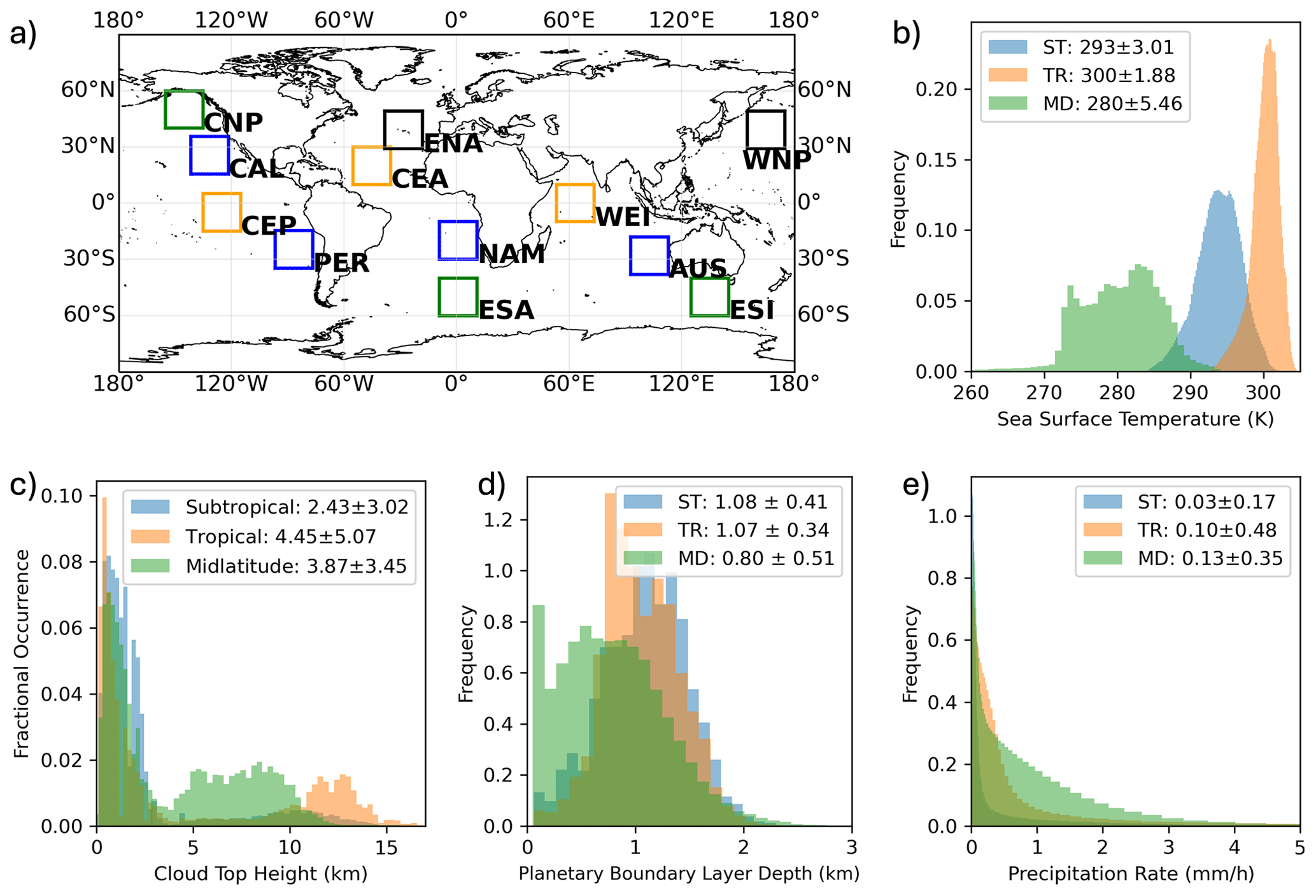
Figure 1 Oceanic regions 20° × 20° in domain size (a) are displayed. The combined subtropical (ST) regions include California (CAL), Peruvian (PER), Namibian (NAM), and Australia (AUS); the tropical (TR) regions include Central East Pacific (CEP), Central Atlantic (CEA), and Western Indian (WEI); and the mid-latitude (MD) regions include Central North Pacific (CNP), Eastern South Atlantic (ESA), and Eastern South Indian (ESI). Mixed regions – Eastern North Atlantic (ENA) and Western North Pacific (WNP) – are not included in the histograms. MERRA-2 Sea Surface Temperature (b), MODIS retrieved Cloud Top Height (c), MERRA-2 Planetary Boundary Layer Depth (d), and MERRA-2 Precipitation Rate (e) are determined from 1-year (2010) data. Means and standard deviations of each distribution are provided.

4 Results

4.1 Regions

Twelve oceanic regions are used in this study (Fig. 1a), encompassing the subtropics (California; CAL, Peruvian; PER, Namibian; NAM, and Australian; AUS, similar to Klein and Hartmann, 1993), tropics (Central East Pacific; CEP, Central Atlantic; CEA, and Western Indian; WEI), mid-latitudes (Central North Pacific; CNP, Eastern South Atlantic; ESA, and Eastern South Indian; ESI), and mixed regions (Eastern North Atlantic; ENA and Western North Pacific; WNP), with tropical and mid-latitude regions selected to ensure representation in both hemispheres and alignment within similar latitude belts. The subtropical locations contain a large abundance (greater than 60 %) of warm low-level (below 3 km) marine stratocumulus cloud (Fig. S1). Tropical and Mid-latitude locations also contain substantial amounts of warm boundary layer clouds, but these regions have significant differences in sea surface temperature (Fig. 1b) with much higher amounts of mid and high-level clouds (Fig. 1c). On average, planetary boundary layer depths are significantly lower in the mid-latitude regions but have the heaviest precipitation rates (Fig. 1e) where a long tail (positive skewness) is apparent indicating a higher propensity for heavier rainfall by frequent large-scale storm-track systems. Precipitation rates are also large in the tropics (compared to the subtropics). The diversity in meteorological conditions across regions provides essential test-beds to isolate and study the impact of different cloud states and environmental controls on ACI.

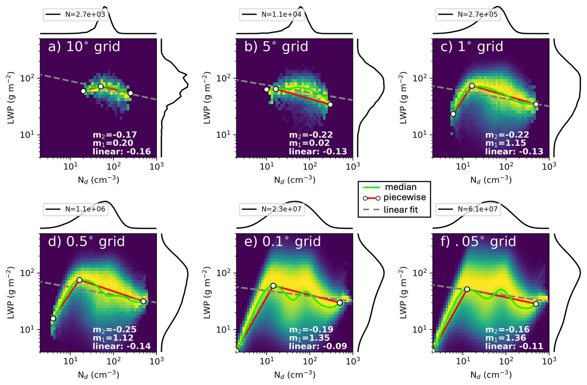
Figure 2 The N_d–LWP relationship is shown as a 2D histogram of joint frequencies, normalized by the total number of binned N_d retrievals, using five years of MODIS data at spatial resolutions of 10° (a), 5° (b), 1° (c), 0.5, 0.1, and 0.05° over a 20° × 20° domain in California (Fig. 1). Black lines indicate the distributions of N_d (top) and LWP (right). Red lines represent piecewise fits to the ascending and descending branches, with slope values (m_n) provided. The gray dashed line shows the linear least-squares fit of LWP against N_d using all retrieved values.

4.2 Impact of grid-spacing

Six spatial resolutions with grid spacing from 10 to 0.05° are used to examine how the shape of the N_d–LWP relationship changes within each region. The total number of grid-cells over the 5 year period in the region increase roughly an order of magnitude for each grid resolution (numbers used in each grid-resolution 7.3×10³, 2.9×10⁴, 6.9×10⁵, 2.6×10⁶, 5.2×10⁷, 1.9×10⁸, respectively). Using the All warm-cloud filter at 1° grid resolution reveals a pronounced inverted-V distribution with distinct ascending and descending branches for the California region (Fig. 2c). This result agrees with Gryspeerdt et al. (2019). As the spatial resolution increases and becomes finer, the inverted-V shape morphs into multiple modes more closely resembling an “M” shape (Fig. 2e and f). The inverted-V shape of the N_d–LWP relationship can be modeled using a piecewise linear function in log–log space, following a similar approach to Gryspeerdt et al. (2019). The function is defined with a single turning point corresponding to the median in the probability distribution function (PDF) of LWP as a function of N_d:

$$\begin{array}{}\text{(1)}& \ln L=\left\{\begin{array}{ll}\ln L_{\mathrm{p}}+m_{\mathrm{1}}(\ln N_{\mathrm{d}}-\ln N_{\mathrm{d},p}),& \text{ if }{N}_{\mathrm{d}}<N_{\mathrm{d},\mathrm{p}}\\ \ln L_{\mathrm{p}}+m_{\mathrm{2}}(\ln N_{\mathrm{d}}-\ln N_{\mathrm{d},\mathrm{p}}),& \text{ if }{N}_{\mathrm{d},\mathrm{p}}\ge N_{\mathrm{d},\mathrm{p}}\end{array}\right.\end{array}$$

Here, N_d,p denotes the turning point – defined as the mode in LWP for a given N_d – with slope coefficients m₁ and m₂ representing the log–log gradients to the left and right of N_d,p, respectively, and L_p the corresponding LWP value at the turning point. At 1° resolution, the N_d–LWP distributions exhibit a well-defined inverted-V structure. However, as spatial resolution increases (e.g., 0.1 and 0.05°), the median of the PDF deviates from this structure and reveals a more prominent “M” shape relative to the piecewise linear fit, reflecting increased subgrid variability. We focus on results at 0.1° resolution in the main analysis to balance computational cost with spatial fidelity, unless otherwise noted.

To explain why the “M” shape emerges at the 0.1 and 0.05° resolutions, a detailed analysis of τ_c and R_e is conducted. Since LWP is proportional to the product of τ_c and R_e (i.e., $\text{LWP}=\mathrm{2}/\mathrm{3}{\mathit{\rho }}_{\mathrm{w}}{\mathit{\tau }}_{\mathrm{c}}{R}_{\mathrm{e}}$, where ρ_w is the density of water), the localized decrease in LWP in the bottom of the “M” trough (Fig. 2e and f), which does not appear in the classic inverted-V shape (Fig. 2c), occurs due to a higher occurrence of clouds with smaller τ_c (Fig. 3b). This change in LWP is primarily driven by variations in τ_c, as the changes in R_e between grid resolutions are similar (Fig. 3c). The statistical differences between these datasets indicate that finer resolutions capture more variability in cloud optical properties, leading to a wider spread in LWP values. This results in a lower median LWP at finer scales due to the increased detection of smaller optical depth clouds.

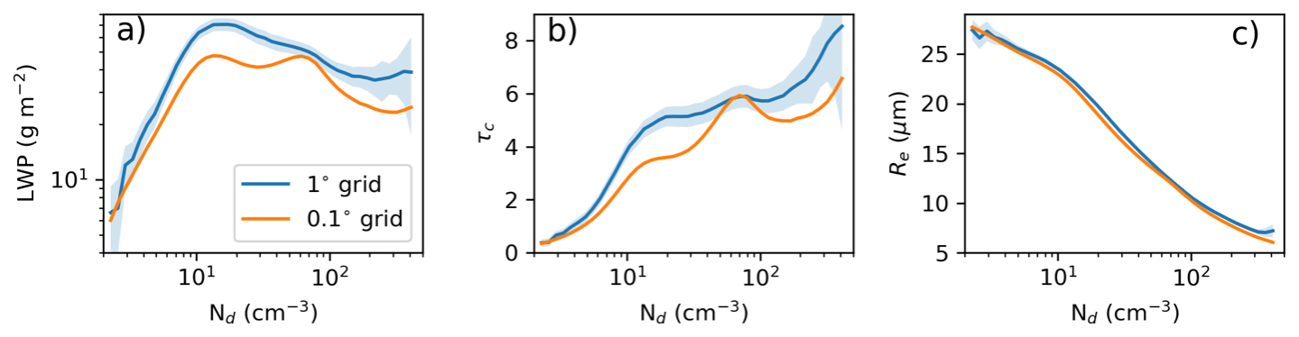
Figure 3 Median LWP (a), cloud optical thickness (τ_c) (b), and droplet effective radius (R_e) from 50 bins increasing by the log in N_d for 5 years of data across the Peruvian region averaged into 1° (blue) and 0.1° (orange) grids.

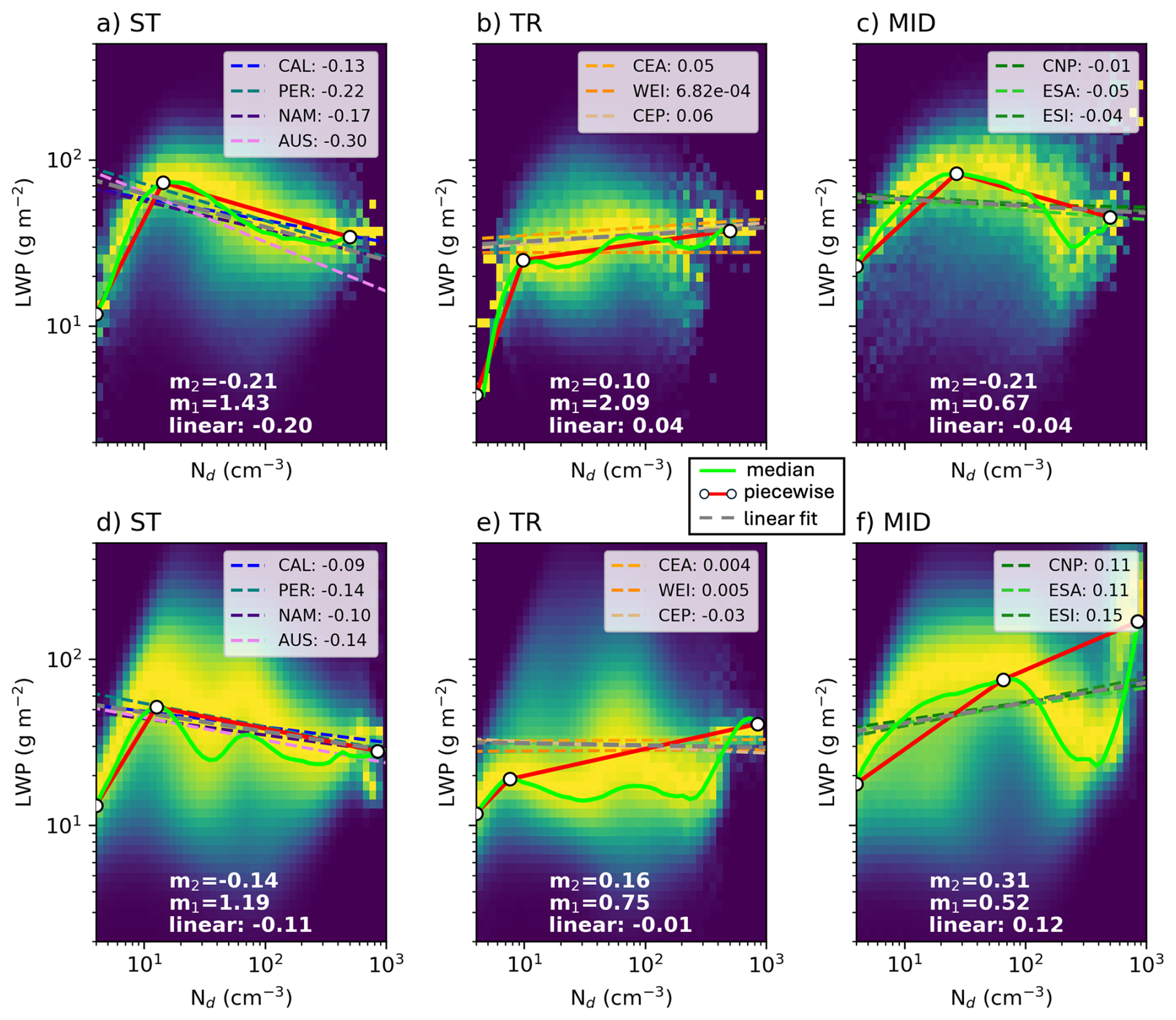
Figure 4 The N_d–LWP relationship expressed using a 2D histogram of the frequency of the LWP and N_d using 5 years of MODIS cloud retrievals aggregated at 1° (a–c) and 0.1° resolutions for combined subtropical (ST), tropical (TR), and midlatitude (MID) locations in Fig. 1. Red lines indicate the piecewise slopes in the ascending and descending branches of the distribution, dashed lines represent the linear least squares fit line for each region.

4.3 Regional Differences

The N_d–LWP relationship varies significantly across subtropical, tropical, and midlatitude regions (Fig. 4). In subtropical regions, a distinct inverted-V distribution with clear ascending and descending branches is evident at a 1° grid resolution (Fig. S2). At higher resolutions, this pattern transitions to an “M” shape, that is robust across all dominant subtropical stratocumulus locations (Figs. 4d and S3). Consistent with Gryspeerdt et al. (2019), the linear-fit slope of N_d-LWP (over the whole range in N_d) is negative in the subtropics at 1° grid resolution. It is also negative at 0.1° grid resolution albeit the slope is significantly less negative at higher spatial resolution. In the tropics, the shapes of these distributions are less pronounced, and LWP exhibits a more neutral/positive trend with N_d. In midlatitudes, the relationship sometimes resembles an inverted-V, but with a significant increase in LWP at high N_d. Linear-fit slopes in midlatitudes tend to be more positive than in the subtropics and tropical regions especially at higher spatial resolution. While the relationships remain broadly consistent within subtropical, tropical, and midlatitude regions, variations in dominant cloud types (which respond differently to aerosols, e.g. see, Christensen et al., 2016), as well as differences in large-scale meteorology and zonal gradients across these domains, can also play a role in shaping the N_d–LWP relationship, a topic we will further explore using ML.

4.4 Impact of sampling and filtering

The accuracy of τ_c and R_e retrievals, which are used to compute LWP and N_d, is generally improved by removing thin and/or broken cloud fields. Thicker overcast cloud fields have less noise from shortwave radiation scattering off a homogenous cloud-scene and more closely adhere to the scattering assumptions inherent in the plane-parallel approximation (McGarragh et al., 2018). A common approach to reduce these errors is to require τ_c to be greater than 4. This more stringent filtering is applied in the Q06 and G18 composites. However, thinner clouds, which are removed in these composites, are generally more sensitive to aerosol perturbations (Platnick and Twomey, 1994).

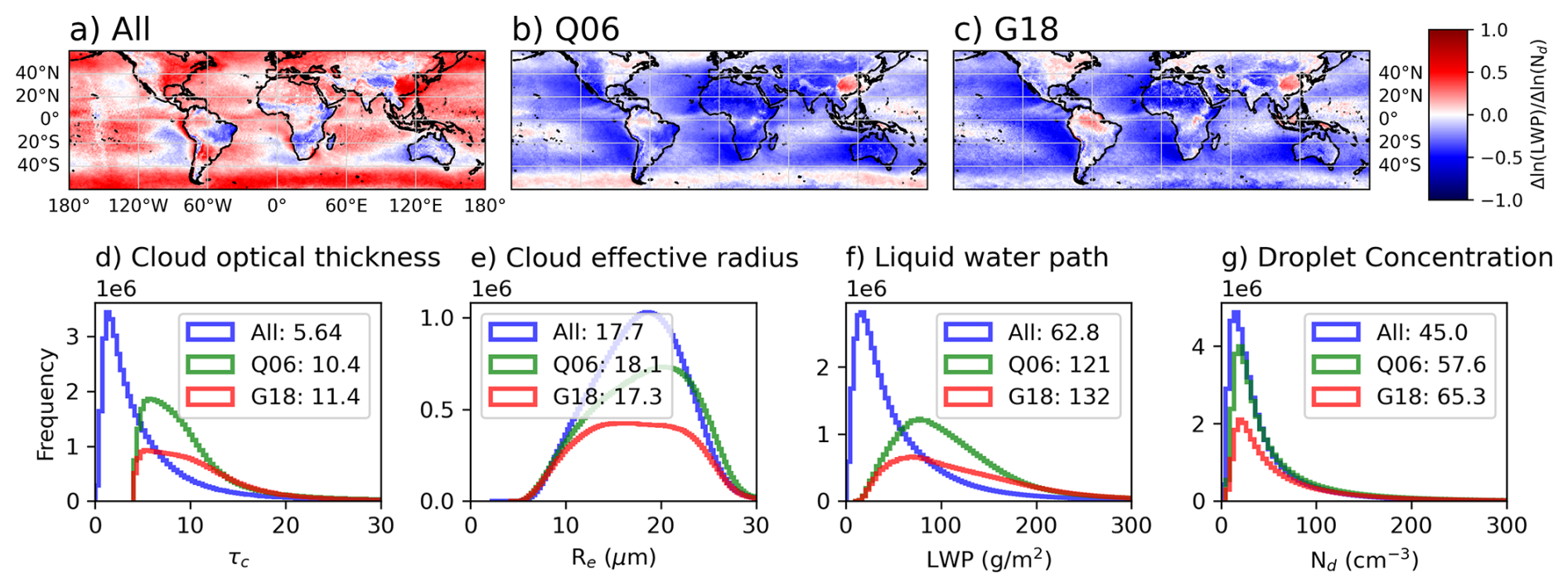
Figure 5 Linear least squares fit between the log of LWP and log of N_d using each composite: All (a), Q06 (b), and G18 (c) for each 1° region of the globe for the 5 year period. Histograms showing the impact of sampling on each composite of τ_c (d), R_e (e), LWP (f), and N_d (g) are displayed.

Figure 5 illustrates the impact of removing thin cloud retrievals from the calculation of the slope in $\mathrm{\Delta }\ln \text{LWP}/\mathrm{\Delta }\ln N_{\mathrm{d}}$ across the globe using the 1° gridded product. When All clouds are included (Fig. 5a), the slope is predominantly positive, except in the subtropics. However, using 0.1° data results in less negative slopes in these regions (Fig. S4), consistent with the observed differences between 1 and 0.1° resolutions in Fig. 4. When thin clouds are removed using the Q06 and G18 composites (Fig. 5b–c), the global distribution of slopes becomes predominantly negative, except in the Southern Hemisphere mid-latitude storm track, Polynesia, and various continental regions. Negative slopes are reported in the literature when applying similar τ_c thresholds (e.g., Fig. 2 in Gryspeerdt et al., 2019, which used the thicker cloud composite of G18). Removing thin clouds reduces the number of cloud retrieval samples by 54 % (Fig. 5d), highlighting the trade-off between reducing retrieval uncertainties and altering the sign of the LWP adjustment.

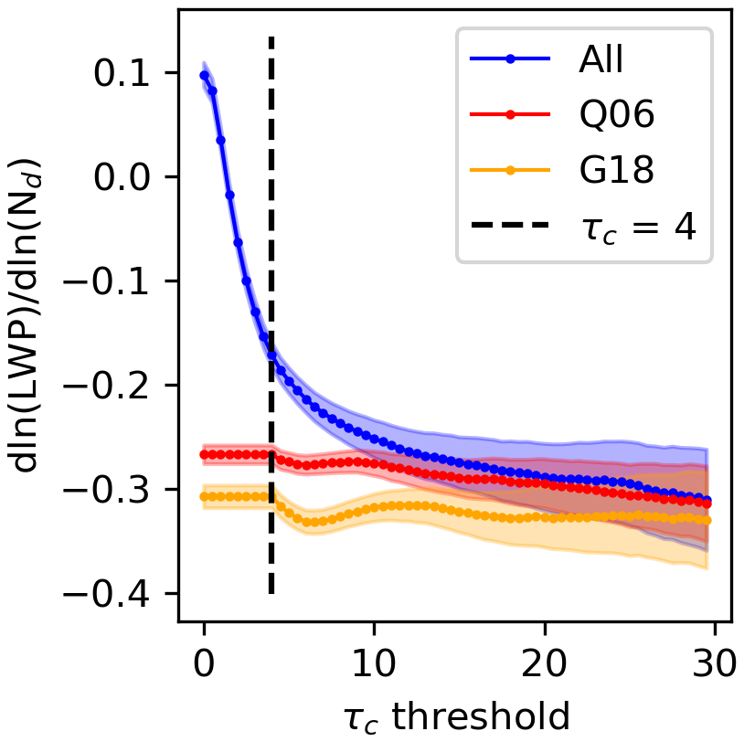
Figure 6 Linear least squares fit between the log of LWP and log of N_d using 5 years of 1° gridded data at the ENA site as a function of increasing the threshold of τ_c. Slope means (circle) for the All (blue), Q06 (red), and G18 (orange) composites are displayed along with the τ_c threshold of 4 used ubiquitously in Q06 and G18.

Figure 6 illustrates the effect of increasing the τ_c threshold on the slope of the N_d-LWP relationship. Beyond an optical thickness of approximately 1.25, the inclusion of thicker clouds with lower susceptibility results in a progressively more negative slope, converging with other composites around an optical thickness of 10. The reliability of cloud property retrievals for thin clouds depends on several factors, including sea state roughness, CF, satellite viewing and zenith angles, and particle size. McGarragh et al. (2018) highlight the challenges of retrieving accurate optical thickness values below 0.1, as subvisible cirrus (optical depth >0.03) can impact the retrieval when they exist (as determined by spaceborne lidar; Reverdy et al., 2012). However, they demonstrate that retrievals are generally reliable for optical depths greater than 1.0, particularly over the ocean, where surface reflectance is well constrained. Given the strong influence of cloud filtering on slope estimates and the significant uncertainties in LWP adjustments, improved constraints on thin clouds are essential for refining radiative forcing estimates. The Q06 and G18 datasets may thus be too conservative and result in overly strong negative slopes. Therefore, to maximize sample size in N_d-LWP relationship, while recognizing the retrieval uncertainties that are intrinsic to thin and broken clouds, we will use the All dataset to assess meteorological impacts in our ML analysis.

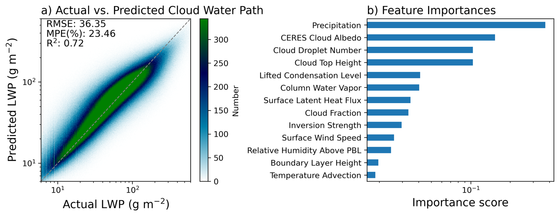
Figure 7 Random forest model predictions of LWP compared to observed LWP using a 25 % holdout testing dataset for the California region at 0.05° grid resolution, with listed values of the Root Mean Square Error (RMSE), Mean Percentage Error (MPE), and Pearson's R-squared correlation coefficient (R²) (a). The relative importance described by Breiman (2001) for each cloud-controlling factor is displayed in (b).

5 Machine Learning the N_d-LWP Relationship

The random forest model is particularly useful for assessing feature importance because it accounts for non-linear interactions between variables, a critical capability given the inherently non-linear nature of the ACI problem. To isolate the impact of meteorology on ACI, a random forest model is used to predict LWP based on 13 cloud-controlling factors (Table S1) in all twelve regions of our study. Figure S5 shows histograms of these factors for the California region, where over 60 million samples from the 0.05° gridded product were used to train the model. It's noteworthy that initially, ∼180 million warm cloud retrievals were available, but requiring joint AMSR-E and CERES observations reduced this to ∼100 million, with additional filtering for ice-free grid boxes further narrowing the sample to 60 million. Figure 7a shows that the model performs very well in predicting LWP when compared to the test dataset achieving a Pearson correlation coefficient squared (r²) of over 0.72. The relative uncertainty in the predicted LWP is ∼25 % compared to the test data. Figure 7b highlights the predictors with the highest correlation values, indicating their importance. In the random forest model, importance is determined by evaluating each feature's contribution to the reduction in impurity (e.g., Gini impurity or entropy) across all trees in the forest, with higher importance scores indicating greater influence on the model's predictions (Breiman, 2001).

Table 1 Performance of the random forest model for predicting LWP over the California region, evaluated using the Pearson's coefficient (R²), mean percentage error (MPE), and the top six variables ranked by importance from highest to lowest.

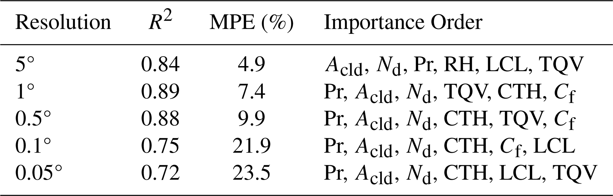
Random forest models with identical hyperparameter settings were trained separately for each grid resolution and each region in this study. Figure S6 and Table 1 shows the accuracy tends to improve with coarser spatial resolution data, however, these coarser grid-resolution have greatly reduced numbers of samples and lack “M” shaped LWP-N_d relationships. The importance of each factor predicted by the ML model are also consistent across regions (Fig. S7). The model also shows robust and stable performance in terms of r², mean percentage error, and the ranking of variable importance across all 12 regions in our study (Table S3). In all spatial resolution datasets (excluding the coarsest), precipitation ranks as the most significant cloud controlling factor for predicting LWP (Table 1). Furthermore, A_cld, N_d, CTH and LCL rank towards the top of the list of “important” variables predicting LWP.

As noted earlier, our selection of hyperparameters and cloud-controlling factors was guided by Chen et al. (2022), Andersen et al. (2023), and Wall et al. (2023). To assess the impact of these choices, we trained the model 100 different times at 0.5° resolution (instead of a higher resolution as this would have been too computationally expensive), varying hyperparameters and predictor combinations and evaluating the model against our validation dataset. Using all predictor variables simultaneously in the training yields the highest r² values (Fig. S8a), while removing single individual predictors has modest effects unless key variables like precipitation, N_d, or A_cld are excluded. Including cloud albedo alongside precipitation significantly improves r² when using only two predictors which is not surprising given the high “importance” of these variables. A minimum of seven samples per leaf node was selected based on how r² responded to increasing this value (Fig. S8b); larger values force the tree to group more data in each decision, resulting in shallower trees with fewer splits, which helps prevent overfitting but may reduce predictive accuracy. Sample fraction, which controls the proportion of training data used to grow each tree, showed little effect on r², so we adopted the default value of 0.6, which introduces some randomness and improves generalization. Increasing the number of trees tends to decrease RMSE and increase r²; we selected 100 trees, where RMSE plateaued and r² approached its maximum value (Fig. S8c), while balancing computational cost, for example, training with 100 trees requires ∼300 % more CPU time than with two trees. Finally, the risk of overfitting, fitting the model too closely to noise or idiosyncrasies in the training data rather than learning generalizable patterns, is likely minimal in our case. The random forest models are small relative to the size and diversity of the dataset, and model skill does not improve at coarser spatial resolutions where overfitting would be most likely (i.e. see Table 1). In fact, performance slightly degrades at the coarsest resolution (5°), supporting the conclusion that the models are not simply memorizing the data.

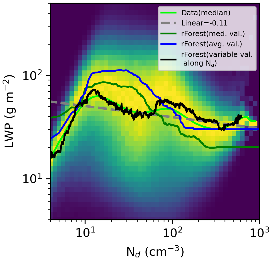
Figure 8 The N_d-LWP relationship displayed as a 2D histogram normalized by the maximum number of retrievals in each N_d bin, using 5 years of MODIS cloud retrievals aggregated at 0.05° resolution for California. The light green line represents the median of the actual data distribution, while the dark green, blue, and black lines correspond to random forest (rForest) model predictions of LWP based on single median values, single mean values, and varying the median of all cloud-controlling factors within each N_d bin, respectively .Linear least squares fit (gray dashed line) and associated slope value is provided.

The random forest model successfully predicts the shape of the N_d-LWP relationship (Fig. 8) thereby enabling detailed examination of the non-linear impact of cloud-controlling factors on LWP. LWP is predicted by the ML model while holding each cloud-controlling variable at a fixed value. When all predictor variables except N_d are held constant (set to either their median values, shown by the green line, or their average values, shown by the blue line in Fig. 8), the resulting LWP distribution exhibits an inverted-V shape as a function of N_d but not an “M” shape. However, allowing the cloud controlling variables to vary with N_d, by using the median value of each cloud-controlling variable for each binned N_d value from 4 to 1000 cm⁻³ reveals the “M” shape (black line in Fig. 8). This suggests that the co-variability of N_d with other cloud-controlling factors plays a crucial role in shaping the LWP response. While Goren et al. (2025) recently highlighted the importance of LWP covariability with other cloud controlling factors, they identified PBLH as a primary driver shaping LWP, whereas our results suggest it plays a lesser role in this relationship with precipitation and cloud albedo being much stronger contributing factors.

5.1 Impact of Precipitation

Precipitation is identified by the ML model as the most influential cloud-controlling factor in predicting LWP. It significantly impacts the N_d-LWP relationship, generally leading to increasingly positive slopes of $\frac{\mathrm{d}\ln \text{LWP}}{\mathrm{d}\ln N_{\mathrm{d}}}$ as precipitation rates increase. The average slope is estimated using both an ordinary least squares (OLS) fit in log–log space and a numerical differentiation approach based on finite differences that computes the mean of local slopes between adjacent points along the random forest predictions as a function of N_d. While the OLS fit captures the overall trend, the finite-difference approach reflects the average instantaneous rate of change, which can differ in shape-sensitive cases such as inverted-V functions. The OLS fitted slope is consistent across all regions (Fig. S9). Furthermore, the random forest ML model accurately captures the shape of LWP as a function of N_d with increasing slopes using finite-differences as precipitation increases across composites (Fig. S10).

Precipitation (probability and intensity) and N_d are closely associated with LWP, typically increasing as LWP increases in warm clouds. While LWP and precipitation generally increase together as clouds deepen, in more developed or heavily drizzling systems, efficient rainout processes can deplete cloud liquid water, leading to a reduction in LWP and a bidirectional response in $\frac{\mathrm{d}\ln \text{LWP}}{\mathrm{d}\ln N_{\mathrm{d}}}$ (e.g., in CloudSat observations of L'Ecuyer et al., 2009; Lebsock et al., 2008; Chen et al., 2014). The ML model supports this effect, showing little variation in LWP with respect to N_d for non-precipitating clouds, likely because increased aerosol concentrations cannot further suppress drizzle in clouds that are already non-raining – yielding a flat or slightly negative response consistent with A-Train observations (Chen et al., 2014). In precipitating clouds, by contrast, higher N_d tends to suppress precipitation by reducing droplet size and limiting collision–coalescence. As shown in Fig. S10c, LWP rises sharply with N_d before increasing more gradually beyond about 20 cm⁻³. The random forest model performs consistently well across all 12 regions, exhibiting a similar pattern of small slightly positive or negative $\frac{\mathrm{d}\ln \text{LWP}}{\mathrm{d}\ln N_{\mathrm{d}}}$ sensitivities for non-precipitating clouds and larger positive sensitivities for raining clouds (Table S3).

5.2 Impact of Cloud Albedo

Cloud albedo plays the next most significant role in modulating the N_d-LWP relationship. Under all-sky conditions, we observe an “M” pattern (Fig. 8), but when stratifying the data into low cloud albedo ($\mathrm{0}<A_{\mathrm{cld}}<\mathrm{0.25}$), average cloud albedo ($\mathrm{0.25}<A_{\mathrm{cld}}<\mathrm{0.4}$), and high cloud albedo ($\mathrm{0.4}<A_{\mathrm{cld}}<\mathrm{1}$), the relationship shifts to solely an inverted-V shape (Fig. S11), even at the highest 0.05° grid-resolution. For dimmer clouds, the peak of the inverted-V occurs at a relatively lower N_d (around 10 cm⁻³), while for brighter clouds, the peak is broader and spans a wider range of concentrations (20–80 cm⁻³), with the LWP shifted to larger values. The linear least squares fit is negative in each composite, while the finite-difference method applied to the random forest predictions yields a weaker average slope due to the pronounced positive increase at low N_d, which is not well captured by the OLS fit. Nevertheless, the consistency of slopes across composites suggests that the influence of precipitation – which tends to steepen the slope – is similar across A_cld groupings.

To test whether the positive LWP response to precipitation is still observed even after compositing the data by A_cld, which drives an overall negative OLS linear regression fit of the N_d-LWP relationship, the data is further composited by precipitation. Figure S12 shows negative slopes of the relationship for the non-raining composites. The slope is especially negative for low-albedo clouds. As precipitation becomes heavier in the drizzle and raining regimes the slopes become more positive and larger in both the OLS and finite differences slopes. This suggests that while the observed negative slope may be shaped by cloud albedo binning, the emergence of a more positive slope is more directly tied to the presence of precipitation. However, it is important to note that cloud albedo itself is not an independent driver of cloud microphysics but rather an outcome of variables such as LWP and N_d, among others. Therefore, interpreting slope changes as being “controlled” by cloud albedo may misrepresent causal relationships and itself serves as a means for binning clouds of varying microphysical quantities.

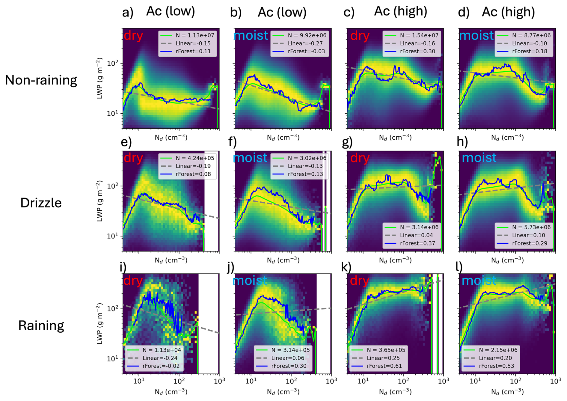
Figure 9 The N_d-LWP relationship is composited by precipitation rate into non-raining clouds ($\mathrm{0}<\text{Pr}<\mathrm{0.05}$ mm h⁻¹; a, b, c, d), drizzle (e, f, g, h), and raining clouds ($\mathrm{0.05}<\text{Pr}<\mathrm{0.2}$ mm h⁻¹; i, j, k, l) for the California region. Within these composites, the data is further divided by low cloud albedo ($\mathrm{0}<A_{\mathrm{c}}<\mathrm{0.25}$) and higher cloud albedo ($\mathrm{0.25}<A_{\mathrm{c}}<\mathrm{1.0}$), and finally by low relative humidity above the boundary layer (dry, red labels) and high relative humidity (moist, blue labels). An OLS fit to the observational data (dashed gray line) and to the random forest prediction (solid blue line), along with the average slope estimated by numerical differentiation of the prediction using finite differences, are displayed.

5.3 Impact of Free Troposphere Humidity

Free tropospheric humidity has often been proposed as a key factor driving negative LWP adjustments (Ackerman et al., 2004; Chen et al., 2014; Gryspeerdt et al., 2019). However, Fig. S13 does not support this expectation, that higher relative humidity leads to a more positive LWP slope as droplet concentrations increase. Based on this first-level binned analysis, LWP appears largely unaffected by relative humidity.

To verify this, we further decompose the response using the most influential variables identified by the random forest method: first by precipitation, then by cloud albedo, and finally by relative humidity. Figure 9 shows that the N_d-LWP OLS slope remains negative for non-precipitating clouds under all cloud controlling factor groupings. For dimmer clouds, A_c(low), higher relative humidity (moist) is actually associated with stronger LWP decreases (not increases) with N_d. Only in drizzling, high-albedo clouds does the LWP OLS slope become positive under an increased RH. If anything, higher free-tropospheric relative humidity decreases LWP. Despite a seeming consensus in the literature (Ackerman et al., 2004; Chen et al., 2014; Gryspeerdt et al., 2019), our findings suggest that relative humidity above the PBL plays a relatively minor role in ACI compared to other factors like precipitation state and cloud macroscopic properties such as albedo in subtropical stratocumulus clouds. This analysis is included to explicitly demonstrate that, contrary to prior expectations, free-tropospheric humidity exerts only a weak influence on LWP. Detailed measurements and/or modeling of cloud top entrainment or divergence may be needed to close this research gap instead of relying on inferred relationships to above PBL relative humidity.

5.4 Radiative Effect

We introduce a new method using ML random forest model predictions for computing aerosol indirect radiative forcing. This approach captures nonlinear relationships between variables, simplifies the computation of partial derivatives while holding other variables constant (e.g. LWP), and eliminates the need for data stratification methods such as binning. The ML model can therefore directly predict the Twomey, LWP, and cloud fraction radiative effects, provided it has been trained with the necessary variables. The shortwave radiative forcing due to a change in anthropogenic aerosols can be expressed as

$$\begin{array}{}\text{(2)}& \mathrm{\Delta }F=-\mathrm{\Delta }\mathit{\alpha }\stackrel{\mathrm{‾}}{F^{\downarrow }}{\mathit{\varphi }}_{\mathrm{atm}}\end{array}$$

where the negative sign denotes that an increase in planetary albedo reduces the net downward (absorbed) shortwave flux, consistent with the convention that positive ΔF denotes a warming (increase in absorbed energy). Here, $\stackrel{\mathrm{‾}}{F^{\downarrow }}$ is the annual mean incoming solar radiative flux at the top of the atmosphere (global mean value of 340.2 W m⁻²), enabling comparison of relative changes in the outgoing flux between regions, and ϕ_atm is a transfer function accounting for the average atmospheric attenuation above the surface and clouds, typically taken as 0.7. The change in planetary albedo due to observed variations in N_d and aerosol index (AI) is given by:

$$\begin{array}{}\text{(3)}& \mathrm{\Delta }\mathit{\alpha }={\displaystyle \frac{\mathrm{d}\mathit{\alpha }}{\mathrm{d}\ln N_{\mathrm{d}}}}{\displaystyle \frac{\mathrm{d}\ln N_{\mathrm{d}}}{\mathrm{d}\ln \text{AI}}}\stackrel{\mathrm{‾}}{\mathrm{\Delta }\ln \text{AI}},\end{array}$$

where $\frac{\mathrm{d}\ln N_{\mathrm{d}}}{\mathrm{d}\ln \text{AI}}$ represents the aerosol-cloud sensitivity, which relates changes in cloud droplet concentration to changes in AI. AI is the product of aerosol optical depth (AOD retrieved at 550 nm) and the Ångström exponent computed using the AOD at 550 and 865 nm wavelength pairs derived from MODIS, which is found to be a better proxy for column cloud condensation nuclei than AOD alone (Quaas et al., 2006). The relationship is positive across our regions with an average value of approximately 0.31±0.16 (Fig. S14). Stronger slopes are typically retrieved in stratocumulus-dominated regions, while weaker slopes tend to occur under more unstable atmospheric conditions with lower cloud fraction. Weaker slopes under these conditions may be partially caused by larger error contributions stemming from satellite retrieval artifacts related to aerosol humidification and 3D scattering effects between clouds with lower cloud fractions (Gryspeerdt and Stier, 2012; Christensen et al., 2017). Higher precipitation rates in tropical regions is also associated with smaller N_d, complicating the causal direction of aerosols and their role on clouds or potentially in this case, the precipitation impact on aerosols as shown in Christensen et al. (2023).

The $\stackrel{\mathrm{‾}}{\mathrm{\Delta }\ln \text{AI}}=\stackrel{\mathrm{‾}}{\ln \left(\frac{{\mathrm{AI}}^{\mathrm{PD}}}{{\mathrm{AI}}^{\mathrm{PI}}}\right)}$ term represents the average log-change in aerosol optical depth due to the influence of anthropogenic aerosols (i.e., based on present-day, AI^PD, and pre-industrial levels, AI^PI). An Earth system model is needed to estimate this quantity. The average value of $\stackrel{\mathrm{‾}}{\mathrm{\Delta }\ln \text{AI}}$ is estimated from 1° spatial resolution E3SM simulations of 5-year average present-day and pre-industrial aerosol emissions, the global results of which are displayed in Fig. S15, and over our regions, $\stackrel{\mathrm{‾}}{\mathrm{\Delta }\ln \text{AI}}=\mathrm{0.41}\pm \mathrm{0.27}$.

The derivative of planetary albedo, defined as $\mathit{\alpha }=(\mathrm{1}-\text{CF}){\mathit{\alpha }}_{\mathrm{clr}}+\text{CF}{\mathit{\alpha }}_{\mathrm{cld}}$, where α_clr is clear-sky albedo, with respect to N_d is carried out using the chain rule expansion described in Bellouin et al. (2020):

$$\begin{array}{}\text{(4)}& \begin{array}{rl}{\displaystyle \frac{\mathrm{d}\mathit{\alpha }}{\mathrm{d}\ln N_{\mathrm{d}}}}& =\text{CF}\left({\displaystyle \frac{\partial {\mathit{\alpha }}_{\mathrm{cld}}}{\partial \ln N_{\mathrm{d}}}}{|}_{\mathrm{LWP},\mathrm{CF}}+{\displaystyle \frac{\partial {\mathit{\alpha }}_{\mathrm{cld}}}{\partial \text{LWP}}}{\displaystyle \frac{\mathrm{d}\text{LWP}}{\mathrm{d}\ln N_{\mathrm{d}}}}\right.\\ & \left.+{\displaystyle \frac{\partial {\mathit{\alpha }}_{\mathrm{cld}}}{\partial \text{CF}}}{\displaystyle \frac{\mathrm{d}\text{CF}}{\mathrm{d}\ln N_{\mathrm{d}}}}\right).\end{array}\end{array}$$

where the clear-sky contribution to the planetary albedo is not included because it is part of the direct radiative effect (i.e. $({\mathit{\alpha }}_{\mathrm{cld}}-{\mathit{\alpha }}_{\mathrm{clr}})\frac{\mathrm{d}\text{CF}}{\mathrm{d}\ln N_{\mathrm{d}}}$ term). All three terms in Eq. (4) represent radiative sensitivities, with the first and second terms restricted to cloudy regions. When combined with Eqs. (2) and (3), these terms correspond to the Twomey radiative effect (where LWP and CF are held constant), LWP adjustment, and CF adjustments. For completeness, the full expression can be written as

$$\begin{array}{}\text{(5)}& \begin{array}{rl}\mathrm{\Delta }F& =-\stackrel{\mathrm{‾}}{F^{\downarrow }}{\mathit{\varphi }}_{\mathrm{atm}}\text{CF}\left[{\displaystyle \frac{\partial {\mathit{\alpha }}_{\mathrm{cld}}}{\partial \ln N_{\mathrm{d}}}}{|}_{\mathrm{LWP},\mathrm{CF}}\right.\\ & \left.+{\displaystyle \frac{\partial {\mathit{\alpha }}_{\mathrm{cld}}}{\partial \text{LWP}}}{\displaystyle \frac{\mathrm{d}\text{LWP}}{\mathrm{d}\ln N_{\mathrm{d}}}}+{\displaystyle \frac{\partial {\mathit{\alpha }}_{\mathrm{cld}}}{\partial \text{CF}}}{\displaystyle \frac{\mathrm{d}\text{CF}}{\mathrm{d}\ln N_{\mathrm{d}}}}\right]{\displaystyle \frac{\mathrm{d}\ln N_{\mathrm{d}}}{\mathrm{d}\ln \text{AI}}}\stackrel{\mathrm{‾}}{\mathrm{\Delta }\ln \text{AI}}.\end{array}\end{array}$$

To implement this framework, three separate random forest models are trained to predict A_cld, LWP, and CF based on the same set of cloud-controlling variables. However, when training the model to predict A_cld, we exclude A_cld as a predictor and replace it with LWP, applying a similar replacement strategy when predicting CF. This approach ensures consistency in the input variables across all models. The performance of the ML models using A_cld and CF predictors (instead of LWP) is summarized in Tables S4 and S5. These models achieve r² values that are comparable to those obtained when predicting LWP. Across most grid resolutions, CF, LWP, and N_d are identified as the most “important” terms influencing A_cld. Similarly, cloud top height, N_d , and the LCL play significant roles in predicting CF.

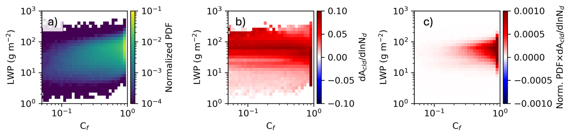
Figure 10 Radiative kernel for computing the Twomey effect using predictions of A_cld from the random forest model for the California region using 1° grid-spacing data. Number of retrievals falling into log-bins of LWP and CF are normalized by the total (a), sensitivity of changes in A_cld for each bin determined using finite differences of the random forest predictions (b), and resulting Twomey radiative kernel (c) given by the product of (a) and (b).

The three terms in parentheses correspond to the Twomey, liquid water path, and cloud fraction radiative effects, respectively. These are multiplied by a radiative scaling factor defined as $(-\mathrm{1}.)\cdot \text{CF}\cdot \stackrel{\mathrm{‾}}{F^{\downarrow }}\cdot \frac{\mathrm{d}\ln N_{\mathrm{d}}}{\mathrm{d}\ln \text{AI}}\stackrel{\mathrm{‾}}{\mathrm{\Delta }\ln AI}$ where the negative sign indicates that an increase in albedo (from higher N_d) reduces the net downward shortwave flux. The first term (Twomey effect) inside the parenthesis, $\frac{\partial {\mathit{\alpha }}_{\mathrm{cld}}}{\partial \ln N_{\mathrm{d}}}{|}_{\mathrm{LWP},\mathrm{CF}}$, is evaluated using a radiative kernel approach, similar to that described in Wall et al. (2023). First, the frequency of occurrence from cloud retrievals within logarithmic bins of LWP and linear bins of CF is estimated from the full dataset (Fig. 10a). Second, the sensitivity of A_cld to N_d is computed within each joint LWP–CF bin, where the random forest model uses fixed values based on the median for each predictor variable corresponding to the midpoints of the bin. Predictions of A_cld are generated across the full range of N_d within each bin and are fit using a linear least squares method (Fig. 10b). To compute uncertainty, the slope within each bin is computed three times using the median values of other cloud-controlling variables and twice more using the median ±1 standard deviation. Finally, the resulting Twomey radiative kernel (Fig. 10c) is calculated from the product of the normalized PDF with the sensitivity summed over all LWP and CF bins (i.e., $\frac{\partial {\mathit{\alpha }}_{\mathrm{cld}}}{\partial \ln N_{\mathrm{d}}}{|}_{\mathrm{LWP},\mathrm{CF}}={\sum }_{i=\mathrm{1}}^{N_{\mathrm{LWPbins}}}{\sum }_{j=\mathrm{1}}^{N_{\mathrm{CFbins}}}{N}_{\mathrm{pdf},i,j}{\left(\frac{\partial A_{\mathrm{cld}}}{\partial N_{\mathrm{d}}}\right)}_{i,j}$). Uncertainties are propagated using the same approach. For the California region, this results in a Twomey radiative effect slope of $\frac{\partial {\mathit{\alpha }}_{\mathrm{cld}}}{\partial \ln N_{\mathrm{d}}}{|}_{\mathrm{LWP},\mathrm{CF}}=\mathrm{0.067}\pm \mathrm{0.0085}$.

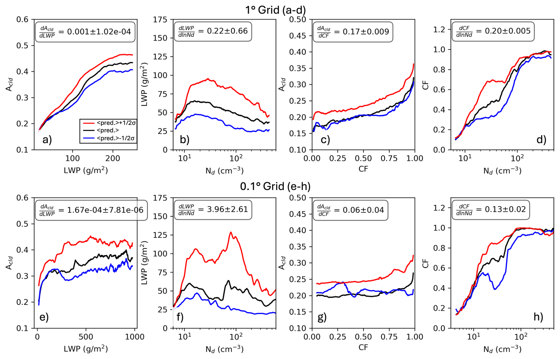
Figure 11 ACI relationships over the California region used to compute liquid water path and cloud fraction adjustments using 1° (a–d) and 0.1° (e–h) grid-resolutions for the relationship between LWP-A_cld, N_d-LWP, CF-A_cld, and N_d-CF predicted using the random forest model. Three different curves represent the relationship using predictions from the median of the cloud controlling factors (black), median +0.5 standard deviation (red), and median −0.5 standard deviation (blue) of the cloud controlling variables. Average and standard deviation of the three slopes estimated by numerical differentiation of the prediction using finite differences are provided.

The next two terms, the LWP and CF adjustment terms, are computed without the need for a radiative kernel since LWP and CF vary with N_d. Figure 11a shows a logarithmic increase in A_cld as LWP increases. (Note, the small scale variability is an artifact of random forest regressors, where averaging outputs from multiple decision trees creates a piecewise constant function that appears smooth, but specific trees cause changes in output nodes as input variables vary, and predictions were made using one RF output per N_d bin with median values of the other inputs for that bin.) This relationship is expected given the analytic two-stream approximation $A_{\mathrm{cld}}\simeq \frac{{\mathit{\tau }}_{\mathrm{c}}}{\mathit{\gamma }+{\mathit{\tau }}_{\mathrm{c}}}$, where γ depends on the degree of forward scattering but for water clouds is approximately 13.33, with ${\mathit{\tau }}_{\mathrm{c}}=\left(\frac{\mathrm{3}}{\mathrm{2}}\right)\frac{\text{LWP}}{R_{\mathrm{e}}}$ (Stephens, 1978). Figure 11b shows the familiar inverted-V relationship (at 1° spatial resolution) with a strong increase at low N_d followed by a peak and decline to larger LWP. The product of $\frac{\partial A_{\mathrm{cld}}}{\partial \text{LWP}}\frac{\text{dLWP}}{\mathrm{d}\ln N_{\mathrm{d}}}$ represents the sensitivity for the LWP adjustment which for California is $-\mathrm{0.016}\pm \mathrm{0.007}$–negative and about 5 times smaller than the Twomey effect. Thus, clouds lose LWP as N_d increases causing A_cld to decrease. Negative LWP adjustments have been identified in natural experiments like ship and volcano tracks (Christensen et al., 2022) as well as in general for warm boundary layer stratocumulus clouds (Gryspeerdt et al., 2019) generally assumed to be caused by enhanced cloud top entrainment and dessication drying of the clouds as they become more polluted (Ackerman et al., 2004).

The CF adjustment is generally associated with much more uncertainty. Observed positive correlations are typically found between cloud cover fraction and aerosol optical thickness. However, these correlations are influenced by physical processes as well as uncertainties caused by artifacts, such as cloud contamination of satellite-retrieved N_d under low cloud fraction conditions, co-variation of cloud fraction with relative humidity/wind speed, and cloud processing of aerosols, which may bias the magnitude of the CF adjustment (Quaas et al., 2010; Grandey et al., 2013). Figure 11c shows that A_cld increases as a function of CF until approximately 0.8, where a sharp increase suddenly occurs as the cloud scene becomes fully overcast. A similar conclusion, albeit replacing A_cld with τ_c (which, using the 2-stream approximation, is a good proxy for A_cld), was also found in Coakley et al. (2005). The rapid rise towards overcast conditions may be a retrieval artifact caused by three-dimensional radiative transfer effects. As the separation between the clouds becomes comparable to the cloud thickness, radiation escaping through the sides of clouds has a high probability of being scattered upward by nearby clouds, thereby contributing significantly to the reflected radiances (Welch and Wielicki, 1985). Figure 11d shows that CF rapidly rises with N_d to about 85 cm⁻³ then flattens out for larger values of N_d. The mechanism behind the increase in CF with N_d has been hypothesized to be due to the reduction in precipitation efficiency, leading to more persistent clouds (Albrecht, 1989) and possibly due to concurrent increases in evaporation and cloud breakup. Gryspeerdt et al. (2016) suggests that the observed correlation may be due to meteorological covariations and artifacts in cloud properties. The product of $\frac{\partial A_{\mathrm{cld}}}{\partial \text{CF}}$ and $\frac{\mathrm{d}\text{CF}}{\mathrm{d}\ln N_{\mathrm{d}}}$ = 0.011±0.01 for the California region. It is positive, suggesting that increased aerosol levels enhance cloud fraction and cloud albedo causing further radiative cooling.

The radiative adjustments are affected by spatial resolution. Figure 11e–h shows that the strength of all the adjustment slopes tend to decrease when using the 0.1° gridded product compared to 1°. The shift from inverted-V to “M” shapes (comparing Fig. 11b with f) is associated with weaker slopes (more positive values). Additionally, the cloud albedo sensitivity to cloud fraction and liquid water path decreases at higher spatial resolutions. These results suggest that data aggregation has a profound influence on the strength of the estimated ACI relationship. Similar conclusions about the grid-scale dependence of ACI have been noted in previous studies (McComiskey and Feingold, 2012; Feingold et al., 2016), but those did not explicitly examine the N_d–LWP relationship, apply machine learning, decompose the radiative forcing into components, or analyze a broad range of satellite grid resolutions at the global scale – further supporting the significance of our findings.

Table 2 List of cloud and radiative effects from aerosol perturbations at increasing grid-resolution for subtropical regions (California, Peruvian, Namibian, and Australian). Radiative scaling is defined as $(-\mathrm{1}.)\cdot \text{CF}\cdot \stackrel{\mathrm{‾}}{F^{\downarrow }}\cdot \frac{\mathrm{d}\ln N_{\mathrm{d}}}{\mathrm{d}\ln \text{AI}}\stackrel{\mathrm{‾}}{\mathrm{\Delta }\ln \text{AI}}$.

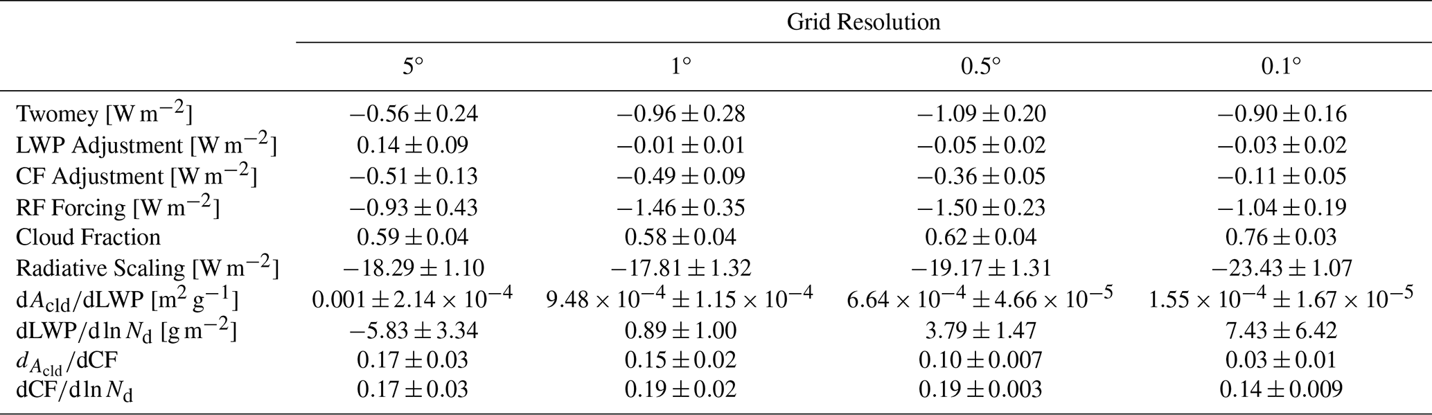
All three terms are now combined using Eq. (5) to estimate the total radiative forcing. Table 2 lists radiative forcing estimates for the combined subtropical regions. Aside from the coarsest resolution, the Twomey effect remains relatively unchanged as a function of grid resolution, with values of approximately $-\mathrm{1}\pm \mathrm{0.2}$ W m⁻². The LWP adjustment contributes very little to the net radiative forcing. At 1° resolution, the CF adjustment makes up over a half of the response, but at finer resolutions, the adjustment terms become negligible. While CF increases on average as a function of grid-resolution (from 0.6 to 0.75), this contribution leads to a slightly larger radiative scaling (since the forcing is proportional to the cloud fraction). However, the primary reason for the reduction in the adjustment terms is the weakened LWP and CF sensitivities to N_d at higher spatial resolutions. While the sensitivities are slightly different between regions (radiative forcing being largest in the mid-latitudes and weakest in the tropics; Tables S6 and S7), these ACI relationships to spatial resolution are similar across regions despite having different meteorological and cloud regimes.

6 Conclusions

We have developed a comprehensive satellite and reanalysis dataset gridded from coarse (10°) to fine (0.05°) spatial resolutions using 3 different commonly used warm-cloud filters (Gryspeerdt et al., 2022) over a 5 year time period. Using this data, a series of outstanding questions that give rise to significant uncertainty in the quantification of ERF_aci and the N_d-LWP relationship have been addressed with the use of ML.

How does the structure of the N_d–LWP relationship change as the spatial grid resolution increases to finer scales?

The structure of the N_d–LWP relationship changes significantly with increasing grid resolution. At coarser resolutions, the relationships found within the subtropics exhibits a classic inverted-V shape. As the resolution becomes finer, the relationship becomes more detailed, revealing multiple modes, including an “M” shape at scales approaching 0.1°. This increase in resolution captures more variability and impact of optically thinner clouds, resulting in a wider spread of LWP values when stratifying by primary cloud controlling variables (like precipitation and cloud albedo) identified using a random forest ML model.

How do subtropical, tropical, and midlatitude regions differ in their N_d–LWP relationships?

The N_d–LWP relationship varies significantly between tropical, subtropical, and midlatitude regions. In subtropical regions, the relationship typically exhibits an inverted-V or “M” shape, with negative linear slopes, which become less negative at increasing spatial resolution. In tropical regions, the relationship does not show these distinct shapes and the linear sensitivity is roughly flat. In midlatitude regions, the relationship is generally positive with less coherent inverted-V or “M” structures, indicating that regional meteorological conditions significantly influence the N_d–LWP relationship.

How does satellite filtering and sampling clouds with different characteristics influence the N_d–LWP relationship?

Satellite filtering and sampling of clouds with different properties have a substantial impact on the N_d–LWP relationship. Including All retrieved warm clouds, which importantly include thin clouds, results in a predominantly positive slope, while more stringent filtering (e.g., removing thinner clouds) leads to mostly negative slopes. Thicker, opaque clouds improve the accuracy of cloud property retrievals but are less sensitive to aerosol perturbations. This indicates that the choice of cloud sampling and filtering criteria can significantly alter the interpretation of the N_d–LWP relationship and its associated radiative effects.

What are the primary meteorological drivers shaping the N_d–LWP relationship?

A random forest model identified precipitation and cloud albedo as critical factors shaping the relationship. Precipitation strongly influences the N_d-LWP relationship, with steeper positive slopes as precipitation rate increases. In non-precipitating clouds, LWP remains flat due to the absence of drizzle suppression, while in precipitating clouds, increasing N_d suppresses rainfall, which increases LWP before leveling off. Binning the relationship by cloud albedo leads to negative slopes of the inverted-V distribution, while precipitation controls the positive slopes. Relative humidity above the PBL has a minor influence on ACI compared to precipitation state and cloud macroscopic properties like albedo.

What is the impact of changing spatial resolution on the radiative effects of ACI?

The Twomey radiative effect is the dominant term, with LWP adjustments being small by comparison; this is consistent with a breadth of observed natural laboratory results by Toll et al. (2019). The radiative forcing is robust across all grid resolutions. On the other hand, the LWP and CF radiative adjustments are strongly affected by spatial grid resolution, wherein the CF adjustment makes up a $\mathrm{1}/\mathrm{2}$ of the response at 1° resolution. Part of the sensitivity decrease is due to shifting from an inverted-V to “M” in subtropical regions, but a larger part of the response is due to a weaker A_cld relationship with LWP and CF as spatial resolution increases.

Estimates of ACI relationships are sensitive to spatial resolution, regional variations, and satellite sampling methods. Associated radiative forcing is impacted by these factors, which underscores the need to evaluate high-resolution, region-specific Earth system model representations of these processes. ML models can enhance our understanding by capturing non-linear effects, identifying key predictors like precipitation and cloud albedo, and offering new capabilities for quantifying aerosol radiative forcing. As Earth system models increase spatial resolution, these data and analyses will be useful for evaluating ACI in warm clouds, which is necessary for identifying model deficiencies and will be addressed in a follow on companion paper.