CloudViT: exploring cloud type classification with vision transformers in global satellite data

Clouds constitute, through their interactions with incoming solar radiation and outgoing terrestrial radiation, a fundamental element of the Earth's climate system. Different cloud types show a variety in cloud microphysical or optical properties, phase, or vertical extent, and thus disparate radiative effects. Both in observational and model datasets, classifying clouds is important since different cloud types respond differently to current and future anthropogenic climate change. Cloud types have traditionally been defined using a simplified partition of cloud top pressure and optical thickness, but recently using deep learning. In this study, we present a method called CloudViT (Cloud Vision Transformer) building on surface observations and spatial extracts of cloud properties from the MODIS instrument to derive cloud types, leveraging spatial patterns with a vision transformer model. The performance of the model is fair and hampered by the limited number of samples and the challenging matching between data sources arising during the colocation process. The method is then evaluated through the distributions of cloud type properties and global spatial patterns of cloud type occurrences. Potential improvements emerge in the reduction in mismatches between data sources, the extension of the colocated dataset, and the refinement of the classification model. While the application of the method in its current state comes with apparent uncertainties due to limited performance, it raises relevant challenges and limitations, from which the community can benefit from discussing for the development of similar methods. To foster future advancements, the dataset and model are available from Zenodo (Lenhardt et al., 2024b).

1 Introduction

Clouds form an essential component in the Earth's climate, by impacting the atmospheric energy budget and water cycle, and by influencing the reflected solar radiation as well as the outgoing terrestrial radiation fluxes. Clouds are highly variable spatially and temporally, and occur in a large variety of types (Howard, 1803; WMO, 2017). Typically, separating clouds between low and high (WMO, 1975), and between stratiform and cumuliform (WMO, 1975, 2017), reveals different and complex cloud effects on processes such as radiation and precipitation formation (Hartmann et al., 1992; Dhuria and Kyle, 1990). The high variability and complexity of clouds are some of the causes for the uncertainties in estimates of their response to anthropogenic climate change both currently and in the future (Boucher et al., 2013; Forster et al., 2021). These uncertainties manifest both in observational datasets for which the aim is to constrain past and current effects, and in climate models where cloud representation is of utmost importance to properly constrain future scenarios. Through the phase (liquid, ice or mixed), the droplet size distribution, the vertical structure or other micro- and macro-physical properties, different cloud types can lead to drastically diverse radiative effects making the cloud type a property of interest to help describe their involvement in the weather and climate system (Ramanathan et al., 1989; Slingo, 1990; Oreopoulos et al., 2017; Luo et al., 2023). Unravelling and understanding trends in clouds has become more tractable in recent decades due to the large amount of remote sensing data made available globally on a daily basis. However, analysing such extensive datasets manually becomes challenging, especially with the goal of extracting meaningful information about different cloud types based on their patterns, microphysical properties or radiative effects. Algorithms have taken over this complex task but still struggle to provide objective groupings out of the intricate spatio-temporal patterns observed in remote sensing data. At the same time, applying methods which are engineered on remote sensing data to climate models could become more viable as new global climate models are bridging the gap in resolution by reaching km-scale resolutions, though this transfer to climate model data comes with its own challenges.

Traditional cloud classification methods are built on simple characteristics. The standard classification developed as part of the International Satellite Cloud Climatology Project (ISCCP) relies on three levels (low, medium, high) of cloud altitude using as proxy the cloud top pressure (CTP) and three thresholds of cloud optical thickness (COT), defining overall nine cloud types (Rossow and Schiffer, 1991). This classification is performed on scalar fields, setting aside any spatial pattern in the cloud field from which information could be obtained to better inform the classification process. Relying on the same type of two-dimensional histograms, recent methods have been developed aiming at refining the created clusters and partially relaxing the constraints on the pre-defined thresholds (Tzallas et al., 2022). The reason to choose the two parameters is that such a classification lends itself to the analysis of cloud radiative effects: the cloud radiative effect in the solar is a monotonic function of COT, the one in the terrestrial spectrum, of CTP. However, one might be interested in sensitivities of cloud thickness or water content to different drivers (e.g., aerosols) for given cloud types, which is hampered by using CTP and COT to define the types. Also, COT does not map well onto the distinction between cumuliform and stratiform clouds. For such reasons, Unglaub et al. (2020) defined cloud regimes from cloud base height and variability in cloud top height, hinting at the added value of some measure of spatial variability and pattern. However, to leverage spatial structure and textures, cloud classification methods based on artificial intelligence (AI) have opened new avenues of research built upon vast amounts of remote sensing data. For example, using convolutional neural networks (CNNs; LeCun et al., 1989; LeCun and Bengio, 1998), Zhang et al. (2018) use ground-based images and human-labelled cloud types to develop a model for meteorological cloud classification and support weather prediction tasks. Using a similar architecture, Rasp et al. (2020) classify clouds from expert-labelled satellite images of four different cloud organisation patterns in the trades. This method further emphasises how expert knowledge to identify cloud patterns can be learned by CNN models and allow to then better constrain radiative effects of mesoscale convection (Wood and Hartmann, 2006; Bony et al., 2020; Stevens et al., 2020) which would prove to be too cumbersome manually. The application of deep learning to the classification of mesoscale cloud patterns in particular (Muhlbauer et al., 2014; Yuan et al., 2020; McCoy et al., 2023) additionally demonstrates how specific cloud organization patterns, observable by experts in satellite data, can be learned by machine learning models, and allows a deeper analysis of their radiative effects and characteristics on longer time periods and larger spatial scales. These studies rely on human observers to initially classify clouds or cloud patterns directly from images, relying on visual aspects to distinguish clouds, and subsequently linking the identified cloud types to local meteorological conditions. Kuma et al. (2023) also capitalize on ground-based observations but connect them to shortwave and longwave radiation satellite retrievals at coarser spatial and temporal resolutions. The method relies on identifying patterns directly in radiation retrievals to associate them to daily occurrence probabilities of cloud types. This method has the benefit of being able to be used on outputs from large ensembles of global model simulations and reanalysis datasets which cover extended time-scales compared to observational datasets. Relying on similar model architectures, Zantedeschi et al. (2019) and Kaps et al. (2023) classify cloud types derived from active remote sensing labels. The study from Kaps et al. (2023) capitalizes on the model from Zantedeschi et al. (2019) to extrapolate cloud type estimates using global passive remote sensing data, and jointly trains a model on coarsened data with spatial resolution similar to current global climate models. Other methods have been developed without the use of cloud type labels, drawing conclusions from clusters appearing in large remote sensing radiation retrievals (Kurihana et al., 2022). In general, the developed methods rely on identifying characteristic patterns arising in images (related to visible features of cloud types), radiation retrievals (related to radiative properties of cloud types), or cloud properties retrievals (related to physical properties of cloud types). Each choice of cloud type labels introduces a certain level of subjectivity in the derived cloud types. For example, there is less subjectivity in the expert-labelled images than in the produced cloud clusters, which naturally introduces some subsequent biases. Choosing certain input quantities also physically constrains the variability of cloud type properties which can hinder the interpretation of the derived cloud type estimates. However, the transferability to global climate model outputs is a great advantage of some of these methods as they provide a crucial way to diagnose the representation of clouds in climate models and push towards reducing uncertainties in representing future-climate clouds (Kuma et al., 2023; Kaps et al., 2023).

Table 1 Datasets description. The surface observations are provided by a worldwide station network available from the UK MetOffice (Met Office, 2006, 2008; see Sect. 2.1). The MODIS data are derived from the collection 6.1 of the datasets (Ackerman and Frey, 2017; Platnick et al., 2017; see Sect. 2.2).

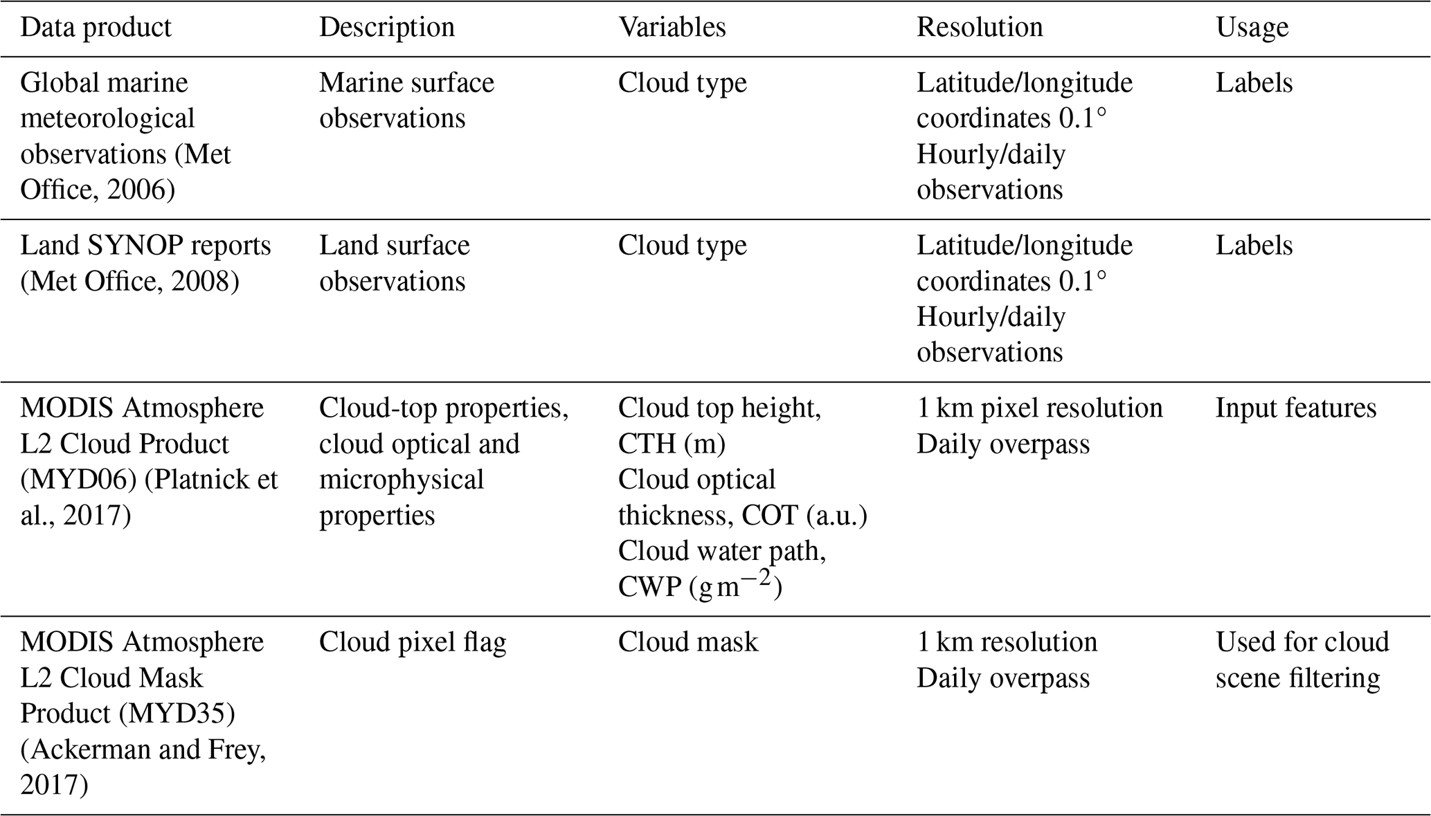
In this study, we investigate the classification of clouds by merging surface observations of cloud types and passive satellite retrievals of cloud properties, building a method called CloudViT (Cloud Vision Transformer). Following a similar methodology from previous work (Lenhardt et al., 2024a), we define cloud scenes as tiles of 128 pixels × 128 pixels which encompass cloud microphysical and optical properties at a 1 km horizontal resolution. The employed cloud properties are from the MODerate Resolution Imaging Spectroradiometer (MODIS, Platnick et al., 2017), and more particularly the cloud top height (CTH), the cloud optical thickness (COT) and the cloud water path (CWP), which are paired with surface network observations of cloud types (cf. Table 1). To harness the spatial aspect of the cloud scene and extract relevant features from the input cloud properties, we resort to computer vision models based on CNNs and transformers (Dosovitskiy et al., 2020). Firstly, a vision transformer model is trained in a self-supervised setting to create a condensed latent representation of the input cloud field. Subsequently, a simpler classification model is fitted to predict the cloud type corresponding to the cloud scene, learning from the labels of a wide ground-based observation network. The formulated method has the goal to produce estimates of cloud types while generalising from the local ground observations to global distributions, increasing both the temporal and spatial coverage. The method relies partly on the assumption that the observed cloud types exist on scales similar to the extent of the tiles, and additionally builds on the spatial patterns characteristic of different cloud types. Moreover, as the ground-based cloud type observations provide consistent labels which are only available at sparse locations, we can leverage long-standing instruments like MODIS to design an algorithm based on satellite retrievals suited to generalisation to global distributions.

Firstly, we introduce in Sect. 2 the different datasets used in the study alongside the colocation process between the ground-based and satellite datasets. Subsequently, the different components of the CloudViT method are presented in Sect. 3, supported by sensitivity studies about the generalisation skill of the models and the benefits of the spatial context. In Sect. 4, we evaluate the method and investigate the distribution of cloud properties following the predicted cloud types. The results in Sect. 5 focus on the extension to a global distribution of cloud types. Challenges, limitations, and lessons learned from CloudViT's development are highlighted in the following Sect. 6, with the guiding idea of making cloud type classification with vision transformers reliable, capable of achieving notable performance, and potentially applicable to high-resolution climate model simulations. Eventually, we conclude over the presented method and challenges of cloud type classification.

2 Data

2.1 Surface observations

The cloud type observations used in this study come from two similar global observation datasets maintained by the UK Met Office, one providing observations made at sea (Met Office, 2006) and the second providing observations made on land (Met Office, 2008). These observations are performed from weather stations (land or sea) or ships, by trained observers following the WMO code tables (WMO, 2019). Each cloud level (high, WMO code table 0509; medium, WMO code table 0515; low, WMO code table 0513; see Table A1) is separated in 9 different types describing in more detail the aspect and type of the observed clouds. The labels thus provide a high level of detail regarding the observed cloud scene from the surface. Naturally, the case of multilayer clouds poses a problem since the field of view and the visibility from the surface are limited, which is why we remove the potential multilayered cases from the training dataset to focus only on single-layer observed cloud scenes. It induces potential selection bias issues as some cloud types might more likely be observed in multilayered configurations. The relative amounts of each cloud type before and after the filtering and colocation process are displayed in Fig. 2. Similarly, uncertainty is greater for medium and high clouds as their observation can be more challenging than for low clouds. Furthermore, the spatial distribution of the labels (Figs. 1 and A1) can be problematic as the marine observations are distributed mainly along ship routes. On the other hand, combining that with land observations provides a more complete representation of cloud types, especially for high level ones, all the while introducing the influence of orography. Other studies like Kuma et al. (2023) and Lenhardt et al. (2024a) have built estimates of cloud quantities based on these ground-based observation datasets, overcoming limitations pertaining to incomplete field of view and disparate spatial distribution.

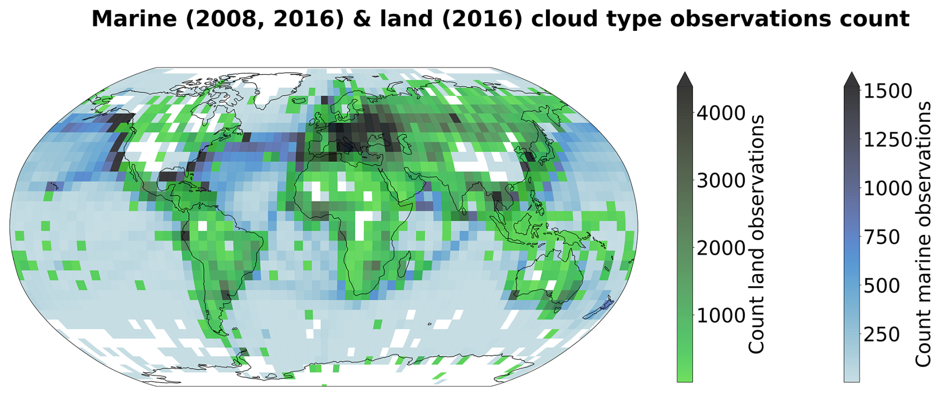
Figure 1 Spatial distribution of cloud type observations for marine (years 2008 and 2016; Met Office, 2006) and land (year 2016; Met Office, 2008). The corresponding spatial distributions of cloud type observations are included in Figs. A1 and A2, for before and after the colocation process, respectively.

For simplifying the analysis but also the training of the classification model, we group the 27 reported WMO cloud types into 4 and 10 categories, similarly to Kuma et al. (2023). The first categorisation allows for broad classification by dividing the cloud species into high, medium, cumuliform and stratiform types. The second categorisation provides a more detailed classification while still limiting the subdivision of similar cloud types. This prevents a too pronounced unbalance in the cloud type labels while possibly removing some of the subjective biases and uncertainty stemming from the human observers. The detailed categories corresponding to the WMO codes are available in Table A1 and shown in Fig. 2.

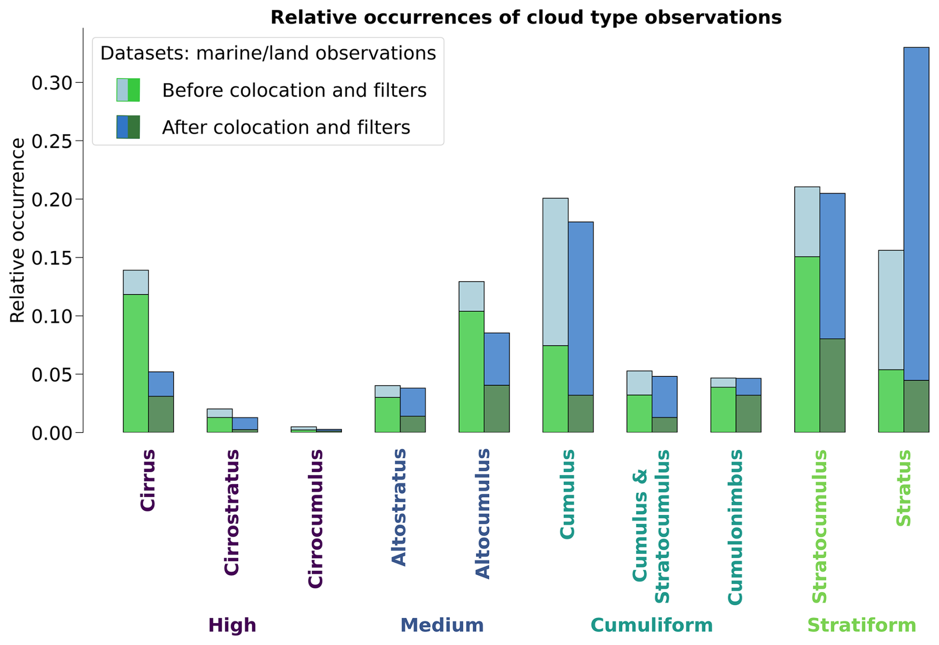
Figure 2 Relative occurrences of cloud types before and after the colocation and filtering process, indicated for both the marine (blue; Met Office, 2006) and land (green; Met Office, 2008) observational datasets. The x axis corresponds to the cloud types in the case of 4 and 10 categories. The corresponding numbers of colocated samples for each cloud type are detailed in Table A1.

2.2 Satellite retrievals

In addition to the surface observations, we use satellite retrievals from MODIS, in particular from the AQUA satellite. MODIS retrievals offer a vast amount of data at kilometre-scale resolution with daily overpasses. Each of the supplied granule file contains cloud microphysical and optical properties across a region with a span of around 2330 km×2000 km. We make use of the available CUMULO dataset (Zantedeschi et al., 2019) since it allows access to preprocessed MODIS level 2 satellite data, with global coverage, and for two full years (2008 and 2016). Among the data variables available, we rely on two unified products (cf. Table 1) describing either cloud properties (MODIS06 level 2 cloud product, hereafter MYD06; Platnick et al., 2017) or the cloud cover (MODIS35 level 2 cloud flag mask, hereafter MYD35; Ackerman and Frey, 2017). The latter's main usage is to help screen for cloud scenes with a minimum cloud coverage.

The MYD06 data product incorporates miscellaneous properties pertaining to the cloud top (temperature, pressure, height) alongside some microphysical and optical properties (effective radius, water path, optical depth). As mentioned previously, our method builds upon level 2 data which are typically obtained from calibrated radiances through methods described in Platnick et al. (2017). More specifically, cloud top properties are retrieved using several radiance channels: harnessing the opacity of CO₂, the CTP of high clouds is retrieved with wavelengths in the CO₂ absorption range, while infrared wavelengths combined with simulated brightness temperatures are used for lower and thicker clouds. The related CTH retrieval can thus suffer from regional biases as the brightness temperatures are based on vertical profiles from reanalysis using regional and monthly averaged lapse rate data along with surface temperature (Baum et al., 2012). The method introduced here can thus incorporate said biases from the input data into the learning process. The microphysical and optical properties of clouds – COT and cloud effective radius (CER) – are retrieved concurrently from multispectral reflectances, CTP values, surface types and cloud masks. Lastly, the CWP is also retrieved as part of the cloud optical properties algorithm detailed in Platnick et al. (2017). The additional input quantities needed to derive and retrieve the mentioned cloud properties (e.g. water vapour and ozone vertical profiles from reanalysis; Platnick et al., 2003; Baum et al., 2012) can result in subsequent uncertainties where only sparse observations like in remote marine areas are available for the data assimilation. Eventually, from the entirety of available MYD06 retrievals, we select three cloud properties in particular, namely the CTH, COT, and CWP.

As a whole, the MYD06 product has the advantage that, building directly on cloud properties, we can design a classification model from which the relationship between cloud type and other cloud properties can then be examined. Relying on calibrated radiances which lie ahead in the retrieval process could offer a more neutral input but due to the large associated dimensionality, extracting information about clouds might become more challenging. Additionally, basing the method on commonly used cloud properties allows us to directly associate the results with other derived cloud classifications, making the comparison and understanding of the predictions more straightforward. Nevertheless, the biases introduced by using level 2 data in comparison to level 1 calibrated radiances and reflectances should be properly characterised and taken into account in the behaviour of the statistical model.

Alongside the colocated dataset, we build a collection of randomly sampled tiles out of the satellite retrievals from the year 2008. For each granule, a maximum of 20 tiles are sampled while ensuring the amount of missing data stays limited. This process leads to the compilation of more than 1.3 M single tiles of cloud properties. These tiles are then randomly split temporally into training (70 %), validation (10 %) and test (20 %) sets. This dataset is the basis for the self-supervised training procedure presented in the following section.

3 Method

3.1 Method outline

Relying on computer vision models and their large number of trainable parameters usually requires adapting the training strategy, particularly when the training dataset is of modest size. In the presented study, the amount of labels available is greatly reduced during the colocation process (see Table A1 for the number of samples per cloud type) but still contains useful and exploitable information about the observed cloud types. We thus introduce a self-supervised learning process which allows us to draw on the larger amount of satellite data available before addressing the more complex task of cloud classification. The larger purpose of this methodology is to be able to classify clouds on a global scale, outside of the areas where surface observations were made and outside of the typical coverage of human observation stations.

For the self-supervised task, we train two models to reconstruct 3D data cubes of cloud properties. The first model, which is used as a baseline, is a CNN backbone we previously presented in Lenhardt et al. (2024a) to handle satellite retrievals of cloud properties for cloud base height prediction. The second model we develop in this study is based on vision transformers (Dosovitskiy et al., 2020), a recent type of model compared to the more typical CNNs for computer vision applications. The spatial pattern of the cloud properties and their scale provide information about clouds, which can be leveraged to classify them for example into more stratiform and more cumuliform types. During the training phase of these models, the samples are images of size 128 pixels × 128 pixels consisting of three different cloud properties: CTH, COT and CWP. We ensure that the models learn to distinguish cloud patterns and not to recognise specific geographical locations by extracting samples randomly across global satellite retrievals from the year 2008, without adding information about their location. In a second step, a classification model is trained on the colocated samples of cloud properties and surface observations. As mentioned in Sect. 2.1, the number of types reported in the observations for clouds is reduced to either 4 or 10 classes (Kuma et al., 2023). The training process follows a supervised learning framework, where the classification model outputs a single cloud type (among the 4 or 10 cloud types) for the whole extent of the input cloud scene of size 128 pixels × 128 pixels. The benefit of the presented method using either a CNN or a vision transformer, which are models incorporating a certain level of spatial awareness, is that it is consistent with the cloud type identified by the human observer. Furthermore, in comparison to conventional methods like the ISCCP, the method benefits from a potential ability to distinguish cloud types without using predefined thresholds.

3.2 Vision transformer

Vision transformers were introduced by Dosovitskiy et al. (2020), building on the transformer architecture previously presented in Vaswani et al. (2017) which was mainly applied to natural language processing (NLP) tasks. The adaptation to images was made by splitting images into patches of a certain size, 16 pixels in the case of the seminal paper, and providing the sequence of embeddings of these patches to a transformer. The patches from the images are then treated as words would be in a NLP application. The transformer can then be trained in a supervised fashion to classify the input images. They have been shown to perform at the same level or even outperform classical computer vision models like ResNets on tasks like classification (e.g. see Sect. 4 of Dosovitskiy et al., 2020). However, as mentioned in Sect. 3.1, this type of model, alongside CNNs, is data hungry and requires a large number of labelled samples to be trained from scratch in a supervised fashion. In this setting, self-supervised pretraining can lead to highly performant models while not requiring a larger training dataset. We train a vision transformer following the self-supervised pretraining methodology presented in Atito et al. (2021), named Self-supervised vision Transformer (SiT). This methodology allows to train vision transformers in a self-supervised fashion building on the concept of Group Masked Model Learning (GMML), additionally using the same autoencoder framework as with traditional CNNs like the commonly used U-Net (Ronneberger et al., 2015) or our baseline model from Lenhardt et al. (2024a). The SiT architecture used in this study is adapted from the seminal vision transformer architecture (Dosovitskiy et al., 2020) by setting the latent dimension to 256, similarly to the CNN architecture introduced in Lenhardt et al. (2024a).

One strength of the transformer architecture is the possibility to easily include several simultaneous learning tasks. We can use this ability to our advantage and incorporate two objectives for the self-supervised training process: input reconstruction following GMML and contrastive learning. The input reconstruction is achieved by adapting the transformer into an autoencoder architecture. Like with traditional CNN autoencoders, the task is for the model to reconstruct the provided input. We benefit further from another advantage of vision transformers as they showcase a reduced complexity compared to CNNs since they rely to a much lesser degree on convolution operations. The methodology of Atito et al. (2021) additionally uses recent results in GMML to further help in the self-supervised learning task. The framework of GMML is integrated in the reconstruction task by replacing random parts of the input image with noise. The overarching goal of this image modification is to train the model to learn semantic representations of the input data, allowing reconstruction of masked areas only with knowledge of some other patches in the input image. The objective for this reconstruction task hence takes the form of the l1-loss, a commonly used metric (Zhao et al., 2016) between the standardised input and the reconstructed output:

$$\begin{array}{}\text{(1)}& L_{\mathrm{r}}={\displaystyle \frac{\mathrm{1}}{N}}\sum _{i=\mathrm{1}}^N\Vert x_i-D_{\mathit{\theta }}\left(E_{\mathit{\theta }}\right(x_i^{\mathrm{c}}\left)\right)\Vert \end{array}$$

where x_i is the input standardised image, $x_i^{\mathrm{c}}$ is the corrupted standardised image, $\Vert \cdot \Vert$ is the l1-loss, N is the batch size, D_θ and E_θ are namely the decoder and encoder parts of the model with θ designating their learnable parameters.

The second learning task included in the training process is based on contrastive learning. Since the presented self-supervised process does not rely on labels for the training data contrary to the vision transformer from Dosovitskiy et al. (2020), the learning task needs to be adapted. To this extent, several geometric transformations and perturbations are applied to the training samples for which the transformer should produce similar outputs. The synthetic pairs can then be used as matching pairs and a metric can be built measuring their similarity. The contrastive task is thus training the model to minimise the distance between matching pairs of sample and corresponding augmented sample, while maximising the distance between different samples in the batch. Atito et al. (2021) propose to use as a contrastive metric the arithmetic mean over the matching pairs in the batch of the cross entropy of their normalised similarities:

$$\begin{array}{}\text{(2)}& L_{\mathrm{c}}=-{\displaystyle \frac{\mathrm{1}}{N}}\sum _{i=\mathrm{1}}^N\log l_{\mathrm{c}}(x_i,x_i^{\mathrm{a}},E_{\mathit{\theta }},D_{\mathit{\theta }})\end{array}$$

where the similarity metric between a sample x_i and its augmented version $x_i^{\mathrm{a}}$ is the normalised temperature-scaled softmax similarity (Chen et al., 2020). The actual process of the contrastive learning further requires the use of a momentum encoder to generate different versions for the pairs of samples and their corresponding augmented samples.

The integral self-supervised training process consists in a combination of the two previously presented learning tasks. For each batch of samples, we create augmented versions of the samples which together constitute matching pairs. GMML corruptions are applied to both samples and the model is subsequently trained to reconstruct the original inputs from these corrupted samples. At the same time, the similarity between matching pairs of samples is maximised. The complete loss function thus takes the form of:

$$\begin{array}{}\text{(3)}& L=\mathit{\alpha }\times L_{\mathrm{r}}+L_{\mathrm{c}}\end{array}$$

where α is a scaling factor between the two tasks. We follow the recommendation of Atito et al. (2021) to set α=5 in the case of small-scale datasets so that the vision transformer can learn enough of the local inductive bias.

We set out to examine in further detail the ability of the vision transformer and of the self-supervised training methodology by evaluating how different configurations of the input data and of the model architecture can impact the quality of the learnt representations and the transfer to cloud classification. We mainly discuss in this section the reconstruction skill of the vision transformer and the potential influence of contrastive learning. The transfer to the cloud classification task will be described in the following section where fine-tuning to the downstream task or the use of external models are surveyed. Since training vision transformers requires large computing resources, we limit ourselves for all the pretraining processes to only 10 % of the initial dataset mentioned in Sect. 2.2, similar to what is done in Atito et al. (2021) regarding ablation studies.

To begin with, we investigate how the two architectures of vision transformers fare during the self-supervised training and how the scaling factor between the contrastive loss and the reconstruction loss impacts the learning process. The two architectures tested correspond to the small variant of the vision transformer from Atito et al. (2021) and the base variant from Dosovitskiy et al. (2020). To offer an overview on each model's complexity, their respective numbers of parameters are 21 and 86 M, the main difference originating from the number of heads in the self-attention layers, the size of the multi-layer perceptron (MLP) and the hidden dimension. We additionally investigate the self-supervised training process by using pre-trained weights made available in Atito et al. (2021) for which the pretraining was done on a computer vision task, the ImageNet-1K dataset (Deng et al., 2009). However, the pretrained weights of the ImageNet-1K dataset are only made available for the small variant of the vision transformer. An additional comparison is done with a model trained only on the colocated dataset using the small variant. The contrastive and reconstruction losses for the different model setups are detailed in Fig. B1. Firstly, we notice that the model trained solely on the colocated dataset would need more epochs to reach similar performance compared to all the other setups. As the colocated dataset contains two orders of magnitude less samples than the training dataset, the model has also seen much less data after 10 epochs, hindering the training process most notably for the contrastive loss. Even after further training the model on the colocated dataset for 150 epochs, it is struggling to match the other models trained on the complete training dataset with best contrastive and reconstruction losses of 0.95 and 0.23, respectively. On the other hand, the other setups reach similar performance in both contrastive and reconstruction losses after 10 epochs. The model with pretrained weights displays better performance right from the start of the training process but improves only marginally thereafter. This could be explained by the fact that using the pretrained weights allows the model to capture already well the structure and patterns of the clouds in the remote sensing data even though their modality is different from the one seen in the ImageNet-1K dataset. It thus shows the strength of transfer learning in computer vision tasks. Nevertheless, we can observe that for the pretrained model both the contrastive and reconstruction losses are reaching a plateau after only a few epochs while the other model setups display a negative gradient indicating further learning capabilities. Focusing on the different variants trained with scaling factors of 1 or 5, we notice that the choice of a larger scaling factor leads to better reconstruction skill while losing almost no performance with respect to the contrastive loss.

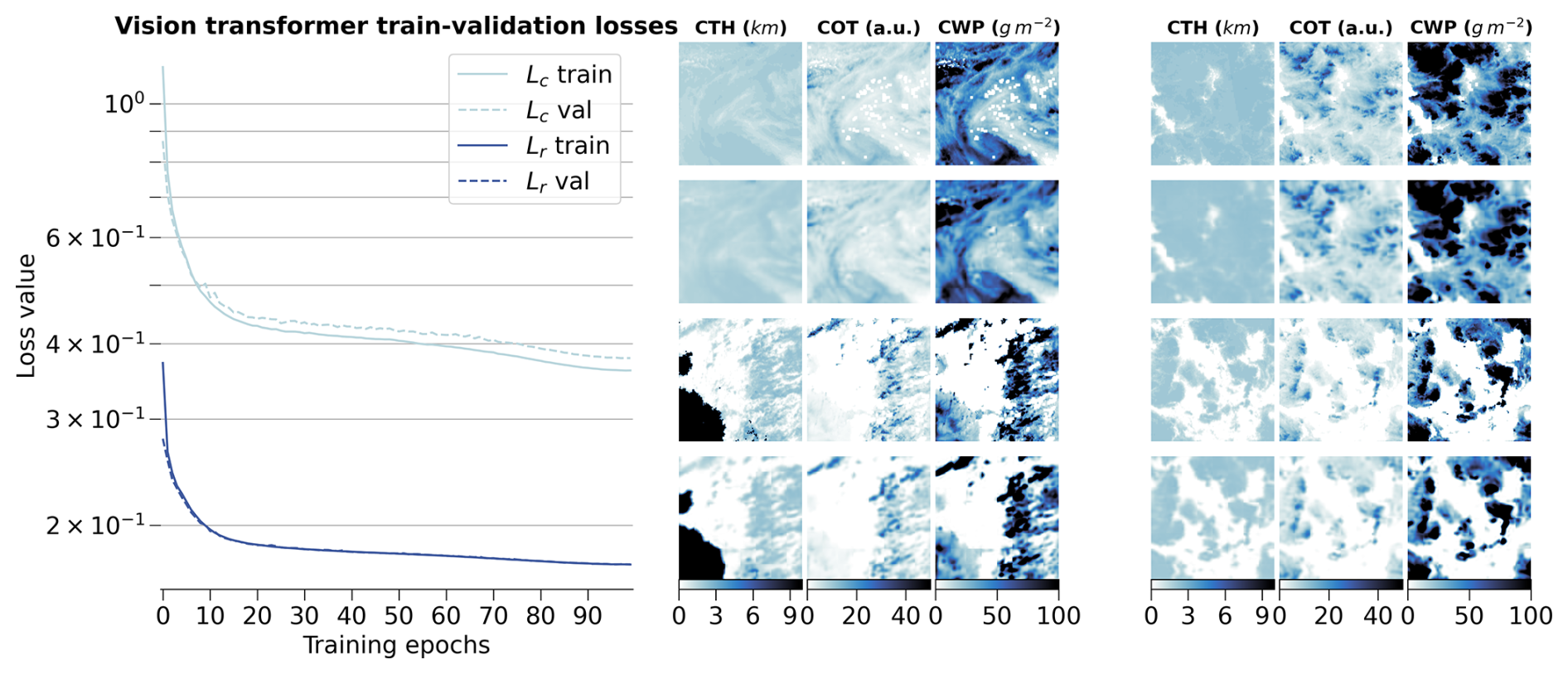
Figure 3 (left) Training and validation losses during model optimization for the small variant of the vision transformer on the global training dataset. (right) Examples of tiles (first and third rows) with the corresponding reconstructions (second and fourth rows) for the different cloud property channels.

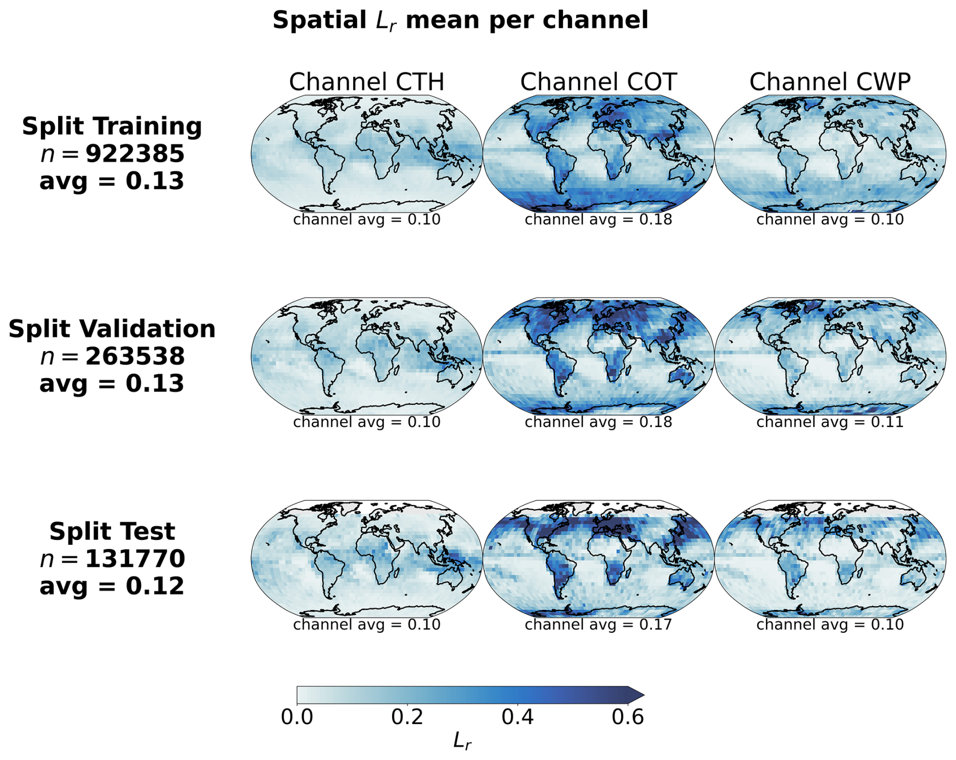
Figure 4 Spatial distributions of mean channel reconstruction errors for CTH, COT and CWP, aggregated on a 5° regular grid for the training, validation and test datasets.

Eventually, we decide to use as model the small variant of the vision transformer with a scaling factor α of 5, as it showcases good performance in both tasks during the training while having a number of parameters four times smaller than the base variant. Furthermore, the self-supervised training task on the large unlabelled dataset allows the model to have plenty of data to learn from, the pre-trained model weights giving only marginal gain for a few epochs at the start. The small variant of the vision transformer was shown to perform very well on a large variety of tasks as per the results from Atito et al. (2021). The results across the training, validation and test datasets are shown in Fig. 3 for the training process and some examples of reconstructed samples belonging to all three splits, while Fig. 4 highlights the spatial distribution of the reconstruction error per channel and across splits. On the left panel of Fig. 3, the losses show a consistent decreasing trend even at the end of the training epochs. The training process was halted after 100 epochs due to computational limitations, but would gain to be extended as the vision transformer's performance seems to still be improvable. On the right panel of Fig. 3, the reconstructions presented for some random samples reveal where the model would benefit from an improved performance: the reconstructions appear realistic, but fail to reproduce the exact sharpness that is visible in the satellite retrievals. While this aspect would not guarantee a decisive improvement in the downstream task which only relies on the encodings, it would greatly help build more trust in the model. A related case that can lead to observed patterns of reconstruction errors in Fig. 4 lies in the reconstruction of cloud scenes with convective cells. The invigorated core of the convective cell stands much higher and holds more water compared to its surroundings which can lead to steep gradients in the cloud quantities when observed from space. As the reconstructions are not able to reproduce these features, larger errors can arise from such cloud scenes. This could further propagate to the classification performance on the related classes, e.g. mesoscale convection clouds or cumulonimbus, whose intricate patterns are better assessed on their own directly (Bony et al., 2020; Rasp et al., 2020; Stevens et al., 2020; Yuan et al., 2020; McCoy et al., 2023). The additional patterns in the reconstruction error of Fig. 4, in particular for COT, are visible in some consistent areas over land. A deeper analysis of the spatial generalisation skill of the model than the one presented in Sect. 3.3.2 covering only the colocated dataset might help constrain the spatial generalisation performance of the vision transformer and infer potential performance caveats still remaining.

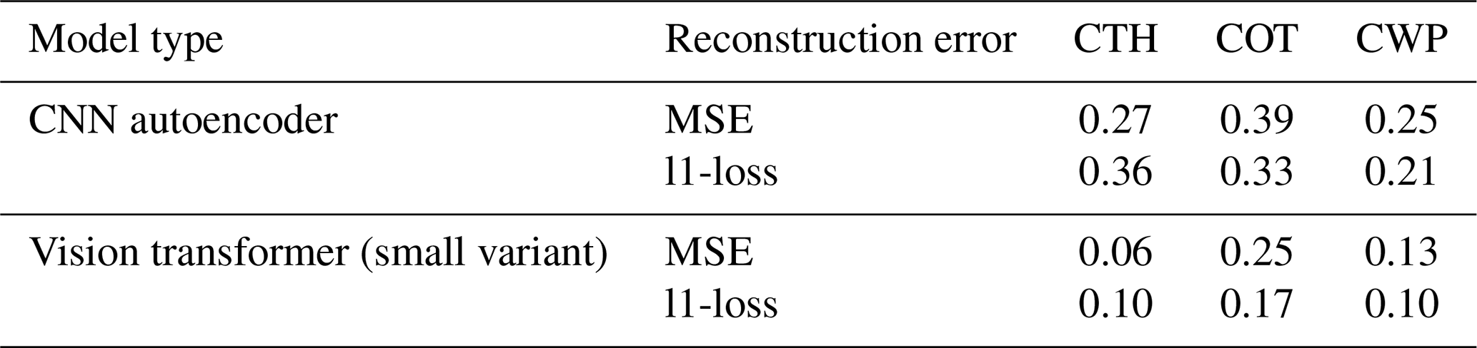
Ultimately, we can compare the skill of the vision transformer to that of the baseline CNN autoencoder from Lenhardt et al. (2024a). The CNN autoencoder was trained using as reconstruction error the mean squared error (MSE) on similar MODIS data but only with MODIS granules over the ocean. It was shown to perform similarly with a slightly higher error over land when evaluated over a global dataset. The vision transformer model outperforms the CNN autoencoder on all metrics (MSE and l1-loss) across all data splits (training, validation and test), displaying consistently across data splits on average an MSE of 0.15 and a l1-loss of 0.12 compared to 0.3 for both metrics for the CNN. Examples of reconstructed samples additionally show how the l1-loss helps produce sharper edges in the reconstruction, a well-known issue with the application of MSE as target metric in computer vision (Zhao et al., 2016). The contribution to the error comes mostly from the COT channel for both models and the error is concentrated in areas of higher variability for the respective channels. The metrics values are summarised in Table B1. The spatial generalisation skill, alongside the sensitivity to the tile size and the impact of data augmentation on the performance on the cloud classification task are analysed in the following section.

3.3 Cloud type classification

The next task at hand is the cloud type classification, building on the colocated samples of satellite retrievals and surface observations. For the two years of MODIS AQUA data available, out of 104 823 colocated samples we retain only 11 094 for our training and testing datasets after filtering, among others, for missing data – typically 50 % of the samples are discarded, mainly when the colocated observation lies on the edges of the satellite granule – and single layer cloud observations as reported by the observer – around 60 % of the previously filtered samples are kept. A main caveat arising from colocating these two data sources is the potential mismatch between the actual clouds jointly depicted. Contrarily to methods like Zantedeschi et al. (2019) which relies on joint retrievals of cloud properties and cloud type or Kuma et al. (2023) which aggregates observations at daily time scales, the presented colocated dataset leaves room for misaligned surface observations and satellite retrievals. As it will be also highlighted later on, this potential misalignment between data sources constitutes a hurdle in the development of the cloud classification method. Indeed, if the model needs to learn from satellite data that actually does not visibly fit the surface observation, then the learning process is hindered. Attempts to reduce this risk have not yielded satisfying results. For example, decreasing the time-window described in Sect. 2.2 did not ultimately yield improvements in the classification performance, especially due to generalisation limitations from a lower number of samples. Furthermore, these attempts are mainly limited by the amount of satellite data that would be necessary to build a substantial and consistent colocated dataset which would span a larger timeframe than the two years used in this study. After the filtering of the colocated dataset, the cloud type observations are then regrouped into 4 or 10 types as mentioned previously. The rest of the study will focus on these categories as targets. From the latent space representations produced by the vision transformer or the CNN autoencoder, we build a classification model either by attaching a classification head to the encoder network or by using a simpler classification model like a random forest (RF; Breiman, 2001). To investigate the performance of the classification models on the two classification tasks at hand (4 and 10 cloud types), we use different metrics tailored to unbalanced classification setups as the cloud types are not equally represented (see Fig. 2 and Table A1). A first method to assign similar weight to all classes regardless of the class' cardinality is to use macro-averaged metrics. In this framework, the metric of interest is averaged over the samples of each class separately before being averaged over the classes. This leads to a higher weight for minority classes for which the model might perform differently, usually worse, compared to the majority classes providing different information over traditional averaging strategies (micro-averaged for example) where the result will be dominated by the samples from the majority classes. We report several metrics adapted to an unbalanced setting: the index balanced accuracy (IBA; Garcia et al., 2012) of the geometric mean, the macro-averaged accuracy and the macro-averaged f1-score.

For the classification model we investigate two alternatives: a RF classification model (implementation from Scikit-learn package, Pedregosa et al., 2011) and a MLP classification head (Hinton, 1989; implemented in PyTorch, Paszke et al., 2019). However, a wider diversity of classification models could be implemented based on the backbone provided by the vision transformer. The base model architecture and weights are made available on Zenodo (Lenhardt et al., 2024b) to foster a more complete exploration of possibilities regarding the classification model, building on the backbone of the vision transformer. For example, with a more extensive training dataset, more complex classification models could be explored. In the case of the architecture presented here,the RF model provides simplicity in the implementation and the training process, while the MLP is the typical architecture used for the downstream task following a network like a vision transformer or a CNN. The RF model has 10 or 25 trees, for the cases of 4 and 10 cloud types respectively, with a maximum depth of 5. Basic hyper-parameter optimization showed that with the reduced amount of samples and the limited variety in cloud scenes for some categories (even more with balanced classes, see Sect. 3.3.3), models displaying limited complexity avoided overfitting and generalised better on unseen data. The MLP consists of two fully-connected layers (hidden dimension 4096) with a Gaussian Error Linear Unit (Hendrycks and Gimpel, 2016) in between and is trained using the cross-entropy loss. The sensitivity studies and experiments are done only using RF models but the evaluation in the subsequent section will be done on both types of classification methods. Various sensitivities could be explored in the presented setting but we here focus on the potential benefit of the spatial context, the ability to generalise spatially to unseen locations and the impact of balancing the labelled dataset.

3.3.1 Spatial context and tile size

We look at the influence of the input size by training vision transformers (small variant) on different sizes of inputs namely 128×128, 64×64, 32×32 and 16×16. We do not consider larger tile sizes as the cloud scene might then be less representative of the surface observation, especially since we only consider samples with single labels, and as the assumption that the observed cloud type occurs on such scales would likely not hold. The losses relative to the vision transformer models trained on the different input tile sizes are detailed in Fig. B2. Since these models were trained on a reduced dataset as mentioned previously, their skill cannot be directly compared to the one displayed in Fig. 3. While the contrastive losses are similar across input tile sizes, the reconstruction losses differ. Since we kept the ratio between the patch size and the tile size constant when training the different models, the difference in reconstruction skill could be attributed to the dimensionality of each patch being much smaller, for example for a tile of size 16×16 a patch will be 2×2. The reconstruction head being a fairly shallow CNN, the reconstruction of the spatial patterns inside the patches showcases better skill for smaller input patches after a few epochs, while for larger patch sizes – and thus tile sizes – a longer training process would be needed as to improve the truthfulness of the reconstruction to the input. Examples of reconstructions depending on the input tile size are included in Fig. B3 and visually display how a larger field of view can help capture the larger cloud organisation or even individual sparse clouds. To further evaluate the potential benefit of the spatial context for the downstream classification task, we consider as an alternate input the flattened cloud properties of a 9×9 tile centred on the observation location. This yields an input of similar dimensionality compared to the latent space representation of both the CNN and the vision transformer (3 channels × 9 × 9 =243). We then train the same RF classification model on each of the latent representations derived from the trained vision transformers and on the flattened cloud properties. From the classification metrics, we observe that the smaller the tile size the more prone the model is to overfitting towards the majority classes (high and stratiform cloud types in the case of 4 types) leading to a decreased performance on the validation set. For instance, choosing an input tile size of 16×16 results in a decrease of 20 % across metrics from the training to the validation set (compared to around 10 %–15 % across metrics for the larger input tile sizes), and leads to metrics on the validation set more than 10 % lower than with larger input tile sizes. The predictions made using larger spatial context (tile size greater than 16×16) outperform the method with 9×9 flattened tile inputs across all considered metrics on the validation set. With the input tile size 16×16, the reduced spatial context seems to be limiting for the performance but another explanation could be a complex latent space compared to the input dimensionality. Overall, even with the vision transformer backbones being trained only partially, the wider input tile size provides better classification skill and generalisation to unseen data. In the rest of the study and experiments, if not mentioned specifically, the input tile size is chosen to be 128×128.

3.3.2 Spatial generalisation

To investigate the spatial generalisation skill of the cloud classification method, we split our colocated dataset into samples located in the Northern or Southern hemispheres. Two vision transformer models are additionally trained on samples from only the respective hemisphere and tested on the other one. The losses relative to the training and testing of both hemispherical models are included in Fig. B4. Both hemispherical models display similar performance both on the training and testing datasets, showing that even for a reduced number of training samples, epochs and spatial coverage the vision transformer architecture generalises well to unseen data. Building on the two trained vision transformers, we set out to evaluate the skill on the classification tasks. Splitting the labels between the two hemispheres yields 9246 samples for the Northern hemisphere and 1848 samples for the Southern hemisphere. Investigating the different classification metrics for training and testing on both hemispheres, it is clear that the classification model trained on the Southern hemisphere struggles to generalise from such a low number of labelled samples and probably overfits since the performance is worsened on the Northern hemisphere samples (decrease of almost 50 % across metrics from the training to the testing set). The classification model trained on the Northern hemisphere generalises well in the case of the 4 cloud types with consistent metric values between hemispheres (marginal decrease of around 15 % across metrics from the training to the testing set). Overall, the model trained on samples from the Northern hemisphere and for both cases of number of cloud types, the performance on the Southern hemisphere is similar to models with larger tile sizes from the previous section, showing consistency across experiments even with limited datasets for the training of the vision transformer.

3.3.3 Balanced training dataset

Balancing the number of samples among classes in the input dataset can be a way to leverage enough information from the underrepresented classes. We compare here the performance skill of two classification models trained on the colocated dataset or on a balanced equivalent. To this extent, we use a sampler implementation from the imbalanced-learn package (Lemaitre et al., 2017), namely the Synthetic Minority Oversampling Technique (SMOTE; Chawla et al., 2002) to oversample the minority classes. Doing so leads to improved classification skill with consistent increases across metrics on the validation set of 3 %–7 % and 15 %–35 % for the cases of 4 or 10 cloud types, respectively. The oversampling impacts mostly the cloud types from the high and medium classes, and from the cirrocumulus and cirrostratus classes, in the case of 4 cloud types and 10 cloud types, respectively (see Table A1). The methods evaluated in the following section will thus include the same over-sampling strategy to overcome the representation of the minority classes and improve the performance on the classification task.

4 Evaluation

4.1 Classification evaluation

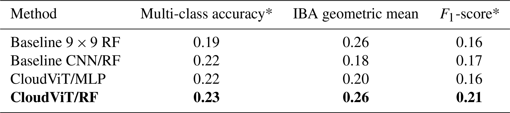
In the following section, we detail the classification performance on the test set of the previously mentioned models. Two baseline models are included, namely a classification model built on the CNN autoencoder from Lenhardt et al. (2024a) and a RF model built on the flattened 9×9 input tiles as described in Sect. 3.3.1. The method developed in this study is represented by two models using the aforementioned vision transformer model (see Sect. 3.2) as backbone complemented by either a RF classifier or a MLP (see Sect. 3.3). In the rest of the study, we denote the trained vision transformer model followed by the classification model as CloudViT (Cloud Vision Transformer) in its two classification variants (RF or MLP). The classification metrics on the test dataset for these four models are summarised in Table 2 for the case of the 4 cloud types and in Table C1 for the 10 cloud types. Since the number of samples is very limited, the performance of the models cannot be only considered as is but is further evaluated in the subsequent sections through distributions of cloud properties and spatial occurrence distributions. We emphasize here the need to perform an evaluation beyond the metrics to assess the skill of the model to represent characteristics expected from different cloud types. These characteristics can relate to the distribution of their physical parameters and their occurrences, both of which can be assessed thoroughly here only with a more extensive dataset. The CloudVit/RF method performs the best across all of the three metrics included, despite showing still limited performance overall. Firstly, the macro-averaged multi-class accuracy does not differ by a large margin between the different methods, but the class-wise accuracies reveal several limitations. The baseline 9×9 RF model largely overfits towards the high and stratiform types (train and test class accuracies of $\mathrm{0.84}/\mathrm{0.81}$ and $\mathrm{0.63}/\mathrm{0.62}$, respectively), performing poorly on the medium and cumuliform types (train and test class accuracies of $\mathrm{0.31}/\mathrm{0.21}$ and $\mathrm{0.19}/\mathrm{0.15}$, respectively). The CloudViT/MLP model is biassed towards stratiform clouds (train and test class accuracy of $\mathrm{0.79}/\mathrm{0.79}$) while struggling to identify the other three types (train and test accuracies all falling between 0.10 and 0.40). The baseline CNN/RF and the CloudViT/RF models are performing quite similarly both on aggregated and class-wise metrics. However, the CloudViT/RF model showcases improved performance on the stratiform class (increase of 0.13 in the class accuracy both on the train and test datasets) and only a marginal decrease (0.03) on the class accuracies for medium and cumuliform clouds. The performance on the high clouds is similar with slightly higher accuracies for the CloudViT/RF model. Other metrics like the IBA of the geometric mean and the F₁-score further emphasise that the CloudViT/RF model outperforms the other methods while addressing the imbalance training data to generalise with satisfactory skill on the unseen test dataset. Nevertheless, the performance detailed here across classes shows apparent limitations as scores are not ideal. An obvious hurdle of the learning process resides in the overall limited number of samples and the noise present in particular for cloud types with minimal numbers of samples. Building a dataset with more labels would improve the classification performance by allowing the classification to more easily converge towards each cloud type's mean state arising from a larger number of samples. The simplicity of the classification models chosen here represents a constraint that could be lifted if more training samples were available as overfitting and balance would then represent lesser issues. Furthermore, the patterns in the class accuracies can be traced back to shortcomings in the observational dataset. Having only considered single-layer cloud scenes in the colocated dataset, the high clouds are well predicted in accordance with the observations as a surface observer would identify with certainty this type of cloud if no other lower cloud is blocking the field of view from the surface. Stratiform clouds could be more challenging for the observers as they typically display high cloud fraction and high optical thickness, limiting the ability of the surface observer to quantify with certainty the amount of clouds in other levels. However, such characteristics can be well captured by computer vision models which build on patterns in the three-dimensional input data which in particular the baseline 9×9 RF model lacks. This difference between models is in particular apparent for the cumuliform class which is mostly composed of observations of cumulus. A cloud scene relative to a cumulus observation will most likely display a lower cloud fraction as the individual clouds are sparsely distributed, extracting only the very near points around the observation might then be too reductive and limit the accuracy of the classification model. It is confirmed by the accuracy on this cloud type for which the baseline 9×9 RF model is largely outperformed by all three other models both on training and test datasets (class accuracy increases between 150 % up to 260 % on the test dataset). Overall, the classification model shows fair performance that could be probably improved by widening the scope of the cumbersome colocation process which requires large amounts of remote sensing data, and by accordingly refining the RF or MLP architectures presented here. Using the classification model developed here thus comes with apparent uncertainties across the different cloud types. Efforts were made with the aim to classify all cloud types consistently from the limited training dataset available but to limited outcomes. The extension of the training dataset appears as an obvious way to purposefully improve the classification performance of the model. An extended colocated dataset would allow stricter filtering, mainly with respect to the colocation time-window, which would help improve the representativeness of the samples. The analysis of the classification performance shows here the limitations of a reduced-size dataset with potential underlying discrepancies between data sources during colocation. Nonetheless, the evaluation of the predictions in the following section provides insights and reveals relevant features in the predicted cloud types.

Table 2 Classification metrics on the test set in the case of 4 cloud types. The metrics noted with a * are referring to their macro-averaged estimate. The method on which the rest of the study is based is highlighted in bold. The baseline CNN/RF refers to the CNN backbone introduced in Lenhardt et al. (2024a).

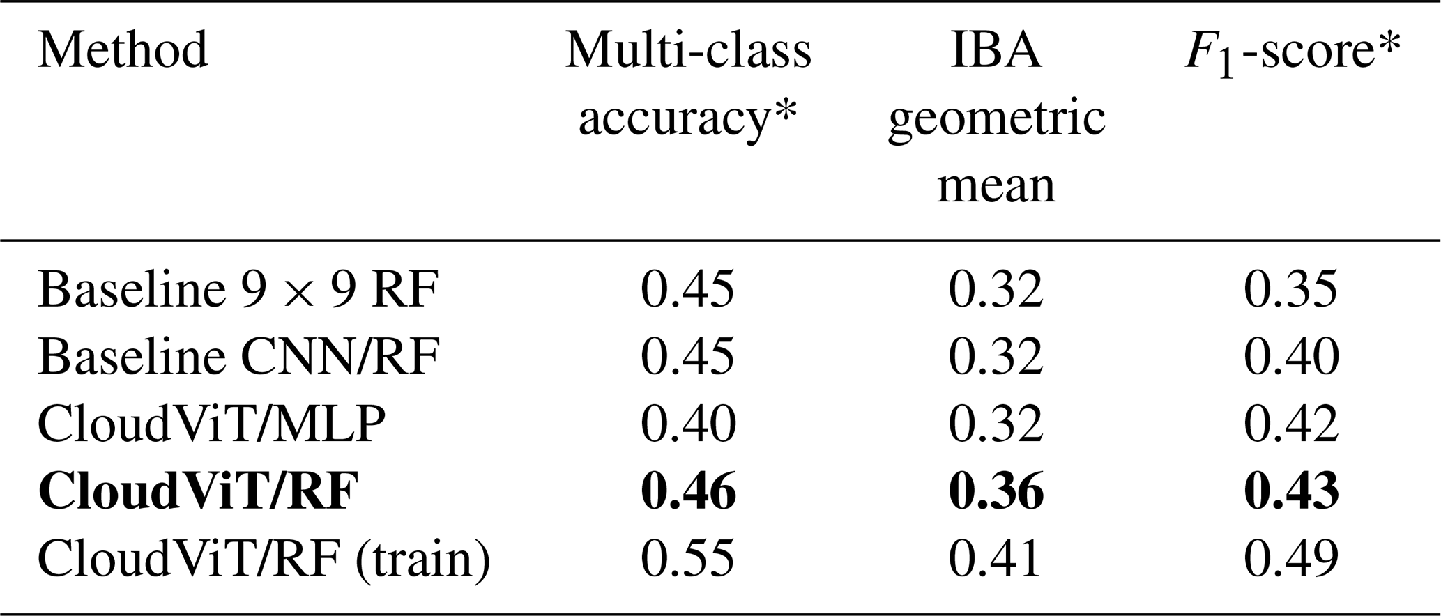
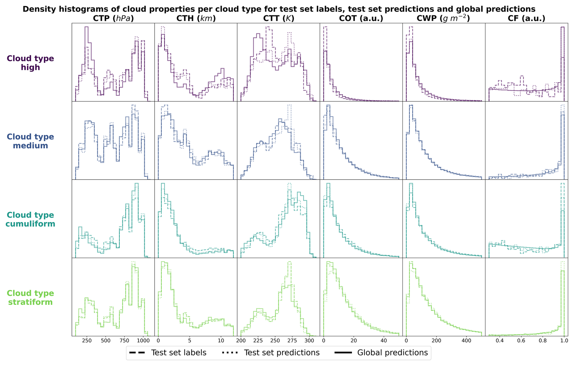
Figure 5 Density histograms of cloud properties for each cloud type from high, medium, cumuliform and stratiform.

4.2 Histograms of cloud properties

In order to evaluate the physical soundness of the predictions made by the CloudViT model, we investigate the distribution of several cloud properties with respect to the observed and predicted cloud types. In Fig. 5, we summarise the distribution of cloud top pressure (CTP), cloud top height (CTH), cloud top temperature (CTT), cloud optical thickness (COT), cloud water path (CWP) and cloud fraction (CF) for the 4 cloud types (high, medium, cumuliform, stratiform) and for three different datasets: the test set labels, the test set predictions and the dataset of global predictions. The latter is built on global MODIS AQUA granules for the year 2016 – the year is chosen to avoid any overlap with cloud scenes seen during the training of the vision transformer on data from 2008 – from which we regularly sample tiles in order to build a more comprehensive and global dataset of cloud types to further evaluate the method. The spatial distribution of cloud types for this dataset is highlighted in the following section and the global dataset is made available at Lenhardt et al. (2024b). The histograms are built by reporting the respective cloud properties for all the cloudy pixels in each sampled tile from the dataset apart from the cloud fraction which is computed for the whole tile from the cloud mask. As a consequence, unless the whole cloud field is composed of only a single cloud type, the histograms will cover a large range of cloud properties due to multi-layer clouds or multi cloud types scenes (e.g. convective cells with associated anvils or cumulus/stratocumulus transitions). Even though the trained model only produces fair evaluation metrics on the test set, the histograms of cloud properties display interesting features consistent with expected characteristics of the different cloud types. On Fig. 5, the histograms pertaining to the test set labels and predictions have distributions close to identical across cloud types showing a good agreement in the clouds depicted in both datasets while the global dataset histograms provides a less noisy overview of the distribution of the cloud properties per cloud type. The high clouds are characterised by low cloud water path and optical thickness, along with colder and higher cloud tops as well as more frequent cloud fractions smaller than one. All of these aspects are emphasised in the global predictions compared to the limited test set samples, showing the CloudViT model manages to extract the representative characteristics of the cloud type from the labels. The cumuliform category encompasses mostly low warm clouds with reduced cloud fractions and moderate cloud water path and optical thickness. Inside this class, the higher and colder cloud tops are concentrated in the cumulonimbus class, along with larger cloud water path and cloud optical thickness (see Fig. C1). The stratiform class includes thick cloud fields with high cloud water path and almost full spatial coverage of the cloud scenes (cloud fraction close to 1 in most cases). A fraction of the clouds in this class are slightly higher and colder and correspond to stratus/nimbostratus clouds which can also be seen in Fig. C1. The distributions for medium clouds showcase similarities with several other types and are best evaluated in combination with their spatial distribution (see Sect. 5). Examining in more detail the refined cloud types with the 10 cloud types (see Fig. C1) reveals slight differences inside broader cloud types. For example, the distinction between the three high cloud types (cirrus, cirrostratus and cirrocumulus) appears through separations in cloud fraction, cloud optical thickness and cloud water path which were not obvious from the limited amount of labelled samples. The differences between the three high cloud types further manifest in distributions of cloud top quantities for which cirrus and cirrostratus display potential multilayered cloud scenes with a combination of low/warm and high/cold cloud tops. Overall, the CloudViT model seems to generalise well from a few samples (only around 10 for the cirrocumulus class) by exhibiting in parts physical consistency inside predicted types. Due to the large cloud scenes considered as input for the classification, the distribution of the cloud properties might not be as representative of single cloud types as an input tile of, for example, 16 pixels. The main caveat regarding performance on high and medium clouds from our method is that the ground-based observer identifies these cloud types with higher uncertainty compared to that of low clouds. Additionally, stratiform clouds with high cloud fraction can hinder the trustworthiness of the surface observation if the whole field of view is cloudy. Even though the limitations of ground-based observations are evident, they still provide quality observations on which a classification model can be trained. The colocation between these surface observations and the satellite retrievals is thus of crucial importance and guides the performance of the later trained model. It partly contributes in the case of CloudViT to a hurdle to achieve notable classification performance. The model, however, shows its ability to generalise from limited samples to consistent and physically-relevant distributions of cloud properties among the predicted cloud types. By refining the training dataset, the improvements can be expected to reflect directly on the classification performance. The characteristics observed in the histograms across cloud types contribute to an increase in confidence in the ability of CloudViT to discern various cloud types in large remote sensing datasets despite the method's limited ability described in the previous section.

5 Global cloud type distributions in MODIS data

Additionally to the physical and microphysical characteristics of the different cloud types, their global spatial distribution can help us further understand in which regions they are more or less frequent and qualitatively assess the presented classification method compared to other remote sensing products. To this extent, as mentioned in the previous evaluation section (see Sect. 4), we build an extensive cloud type dataset for the year 2016 from MODIS AQUA granules which are regularly sampled for tiles of 128 pixels × 128 pixels. The sampling step (64) is chosen for computational efficiency and memory purposes to be not too small to avoid large overlap between neighbouring tiles but large enough to ensure representativeness in the later aggregated predictions of the MODIS granules. Furthermore, as the area covered by each tile is rather wide, the spatial distribution of cloud types might be less smooth than other products (e.g. Sassen et al., 2008) or other methods (Zantedeschi et al., 2019) which are providing cloud types for smaller cloud fields. Additionally, the dataset is built on single daily overpasses of the MODIS instrument and can thus be biassed towards the local retrieval time (13:30 h, early afternoon for AQUA).

The spatial distributions of the predicted cloud types for the global dataset for the year 2016 are detailed in Figs. 6 and C2 for 4 and 10 cloud types, respectively. Firstly, we note that CloudViT predictions capture large scale patterns which are in agreement with observational datasets (Sassen et al., 2008; Cesana et al., 2019; Wood, 2012; Pincus et al., 2023). Stratiform clouds, and in particular stratocumulus (see Fig. C2), are frequent in the high latitudes and along the western coasts of America and Africa. Cumuliform clouds are concentrated in the Tropics apart from the areas where stratocumulus clouds are dominant. Medium clouds are concentrated in the polar regions and over land in the higher latitudes. High clouds make up a large portion of clouds in the polar regions but also over land. The first notable difference is the low occurrence of high clouds in the Tropics which would be expected to be higher (Sassen et al., 2008; Pincus et al., 2023). An explanation could be the frequent occurrence of high clouds in multi-layer cloud scenes related to convection in the Tropics. Furthermore, in such cases the model probably identifies the cloud types with larger cloud fraction and thus discards potential high clouds in the scene. Incorporating more samples of high clouds in that region (see Fig. A1) could potentially help the performance of the classification model in that regard. The presented spatial distributions may suffer from the somewhat limited performance of the classification model despite the corresponding reasonable representation of cloud type characteristics showcased in Sect. 4.2. Nevertheless, some informative features are observed in Figs. 6 and C2 and point towards the good direction for further improving CloudViT.

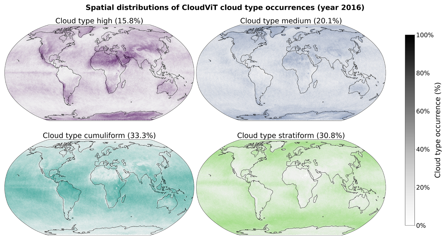
Figure 6 Spatial distributions of the CloudViT cloud type occurrences (cloud types high, medium, cumuliform, stratiform) for MYD06 granules for the year 2016 aggregated on a 1° regular grid.

6 Challenges and limitations

The method and results presented offer a good foundation for further development and critical analysis, though they also have notable limitations that should be addressed.. The following section aims to focus on several aspects that we feel are relevant for the community when developing cloud type classification methods similar to the one presented here, namely on the benefits of such methods, dataset curation and extension, and the potential application to climate model data.

Spatially-resolved cloud properties provide usable context for the CloudViT model to improve the cloud classification, as shown in the comparison to the baseline method with limited spatial information. Introducing this new transformer model architecture additionally improves the classification skill over the CNN backbone mentioned in Lenhardt et al. (2024a). While the performance improvement between baseline CNN and CloudViT is apparent, the overall limited performance of the model stands out, especially when comparing to metrics typically achieved by CNNs or ViTs alike in common classification tasks. Our experiments suggest that the current architecture, while leveraging capabilities of transformers, does not yet fully exploit the organizational and multi-scale spatial features critical for robust cloud type classification. The transformer's self-attention mechanism may require stronger spatial priors (e.g. multi-resolution patch embeddings) to improve the attention of the model to both fine- and coarse-scale features specific to cloud spatial organization. The self-supervised pre-training of CloudViT circumvents this aspect of the ViT architecture to some extent and partly alleviates its data-hungry training process. However, when tackling the targeted cloud classification problem, the limited size of the colocated dataset constitutes a hurdle for the proper training and evaluation of the method on labelled samples. The classification model could also be refined by finding better alternatives to the RF or MLP presented here. The overall finetuning process involving the vision transformer and the MLP classification head proved to be cumbersome but holds great promise if the labels and training process are refined. Transfer learning from a typical ImageNet-trained model did not yield a notable performance difference which shows the current need for foundation models trained on remote sensing data. The main hurdle here remains the large diversity in instruments, quantities and resolutions among remote sensing products which hinders the possibility of a unified model.

Additionally, the hypothesis as to why the model fails to achieve great performance in this study rests heavily on the colocation process between surface observations and satellite data. The method would benefit from including further ground-based observations through the colocation process, but then much larger storage and computational facilities would be needed as global MODIS data represents thousands of granules each day. To further improve the output of the colocation process and the spatial coverage of the CloudViT predictions, the direct application to granules from MODIS TERRA would technically not require much more work as the instruments are similar and provide the same cloud properties. More training samples could simultaneously solve performance issues by providing a clearer vision of the different cloud types for the classification model to learn from. The improvements through a larger training dataset will yield relevant benefits only if the potential mismatches occurring during the colocation process are tackled. Indeed, relaxing some spatial and time constraints during colocation would allow more samples to be retrieved, but it would simultaneously decrease the likely representativeness of the satellite data with respect to surface observation. On the contrary, improving the representativeness of the training samples combined with an extended number of colocated samples could solve the performance issues faced by the model presented here, and potentially achieve performance aligned with a wider usage of the method for cloud type analysis.

Another interesting aspect to discuss here is the application of cloud type classification methods to climate model data. However, the presented method CloudViT would need further improvement on classification metrics before it can be considered to be used on model data with the aim to gain detailed insights into cloud type representation. In general, the application to climate model data can prove to be technically straightforward and can result in practical insights into how such methods can be transferred to model data (see Appendix D). Generally, cloud type diagnostics could be a resourceful addition to the panel of existing assessment methods for model data (Kuma et al., 2023; Kaps et al., 2023). A benefit of using quantities such as cloud top variables or optical thickness as input for the classification method is that these necessary cloud quantities can be obtained from common simulation outputs (cloud liquid water and ice contents, altitude, droplet number). However, some caveats can appear when applying a cloud classification method to climate model data. As mentioned in more details in Appendix D, the input scaling is crucial to ensure proper portability of a method to other data sources. The absence of nighttime retrievals in the MODIS data also turns the evaluation of predictions on nighttime data points across the model data into a challenging issue. However, clouds play a role in the climate system both during the day when they cool the surface by mostly reflecting incoming solar radiation but also at night when they warm the surface by trapping outgoing terrestrial radiation. Shifts and changes in cloud occurrence and distribution in the current climate but also in future projections could further influence global climate change (Luo et al., 2024). Applying a cloud classification methodology to a limited high-resolution climate model simulation is an encouraging direction, but considering more common and computationally less expensive global km-scale simulations (horizontal resolution of 5 km for example) could be of greater interest to the community to study longer time scales. To this extent, two conceivable approaches would consist in either retraining a method on coarser input cloud properties matching the model data resolution – the MODIS Cloud product is also available at a 5 km resolution even though the 1 km equivalent is recommended for use – or in using such a method as is but with the coarse input scaled to fit the resolution of the tiles on which it was trained on. The first option could be more interesting as computer vision models are commonly trained on coarser resolutions first to learn the broad specificity and patterns in the data before fine-tuning the model on finer resolution (Touvron et al., 2019).

7 Conclusion

This study introduces a new method called CloudViT to classify cloud types from MODIS cloud properties, specifically CTH, COT and CWP. CloudViT delivers estimates for either 4 (high, medium, cumuliform, stratiform) or 10 (cirrus, cirrostratus, cirrocumulus, altostratus, altocumulus, cumulus, cumulus and stratocumulus, cumulonimbus, stratocumulus, stratus) cloud types with fair performance. The classification model was built on ground-based observations of cloud types (Sect. 2.1) and experiments about its generalisation skill and the benefits of spatial information were presented (Sect. 3). We evaluated the classification model by examining distributions of cloud properties in Sect. 4 and the global spatial distribution of cloud types in Sect. 5. Lastly, we pinned down some existing challenges, limitations, and lessons learned from the development of the method for cloud type classification. The global dataset alongside the CloudViT code and weights are made available on Zenodo (Lenhardt et al., 2024b) to encourage future developments.

In conclusion, the method presented here showcases and highlights a wide array of potential applications in the study of cloud types, their characteristics and evolution, and their past, current, and future effects on the Earth's climate: from the extension of sparse surface observations to global yearly predictions, and existing challenges and limitations in the design of vision-transformer-based models. Despite the relatively imbalanced performance assessment of the method which shows both great promise in capturing large scale characteristics of cloud types distributions but struggles to capture precisely the features in the training dataset, the design and development of CloudViT is an interesting study in the line of improving existing cloud classification methodologies. Identified challenges and limitations in this particular case can be useful to the community, both in terms of methodology development and caveat to be avoided. We recommend future advancements in cloud classification methods like CloudViT being firstly focused on data curation and followingly on model tuning once the performance has been raised to desirable levels. To this extent, the necessary datasets and model architecture code are made available on Zenodo (Lenhardt et al., 2024b).

Appendix A: Cloud type observations

Table A1 Cloud types from the WMO observational datasets, their groups following Kuma et al. (2023) and the corresponding number of samples in the colocated dataset. The WMO codes correspond to the 9 types for each level.

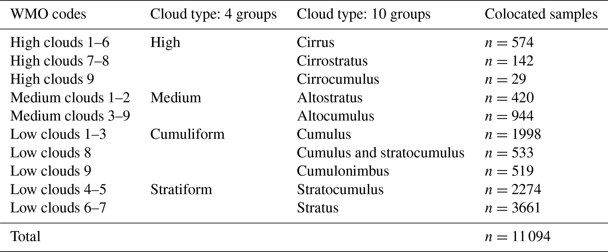
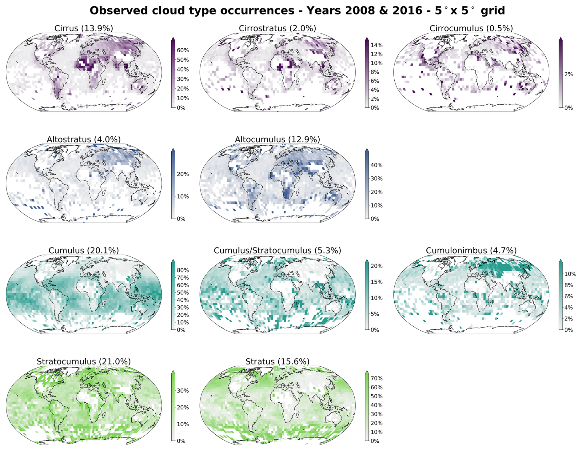
Figure A1 Spatial distributions of observed cloud types (cloud types cirrus, cirrostratus, cirrocumulus, altostratus, altocumulus, cumulus, cumulus and stratocumulus, cumulonimbus, stratocumulus, stratus) from the Met Office datasets (Met Office, 2006, 2008) for the years 2008 and 2016. Overall percentage of each label in the total dataset is indicated in brackets.

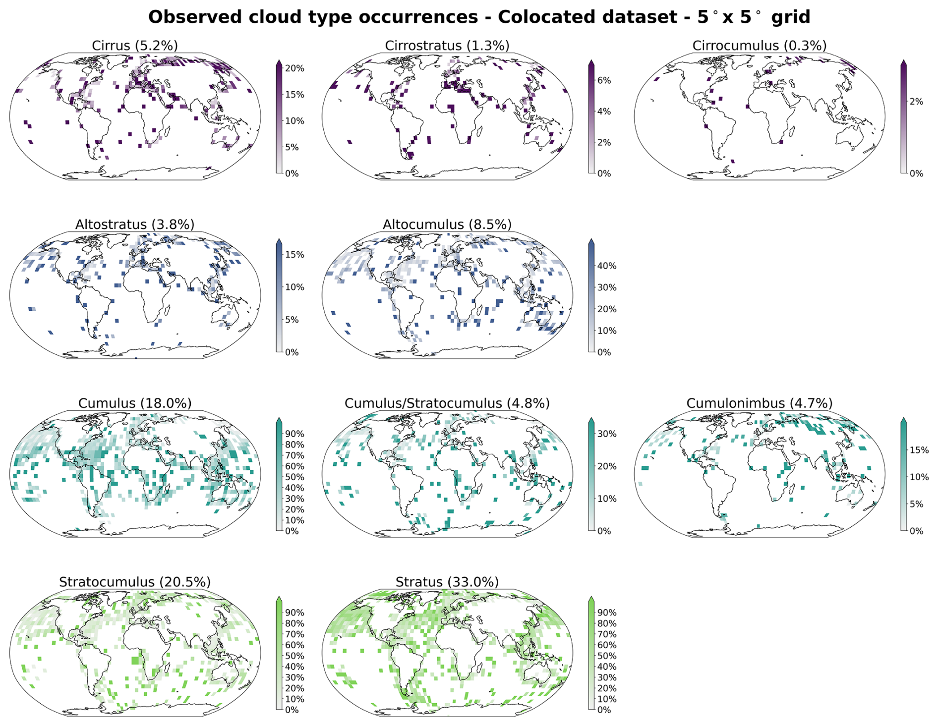
Figure A2 Spatial distributions of observed cloud types (cloud types cirrus, cirrostratus, cirrocumulus, altostratus, altocumulus, cumulus, cumulus and stratocumulus, cumulonimbus, stratocumulus, stratus) from the Met Office datasets (Met Office, 2006, 2008) for the years 2008 and 2016 colocated with the satellite cloud retrievals (Platnick et al., 2017) used for training the classification model. Overall percentage of each label in the total dataset is indicated in brackets.

Appendix B: Vision transformer training and sensitivity on the cloud classification task

B1 Model architecture and pretrained weights

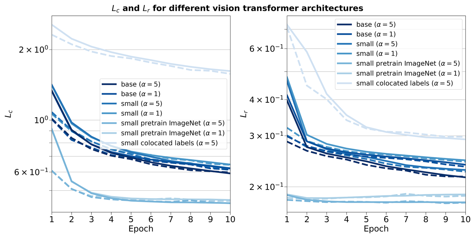
Figure B1 Training and validation contrastive (left) and reconstruction (right) losses for different vision transformer architectures, pretraining weights, training datasets and scaling factor α.

B2 Reconstruction errors for the CNN autoencoder and the vision transformer (small variant) on the test set

Table B1 Reconstruction relative errors of the CNN (Lenhardt et al., 2024a) and the vision transformer models across channels (CTH, COT and CWP) on the test dataset.

B3 Spatial context and input tile size

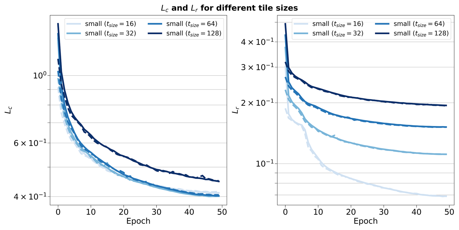
Figure B2 Training and validation contrastive (left) and reconstruction (right) losses for vision transformers trained on different input tile sizes of 16, 32, 64 and 128.

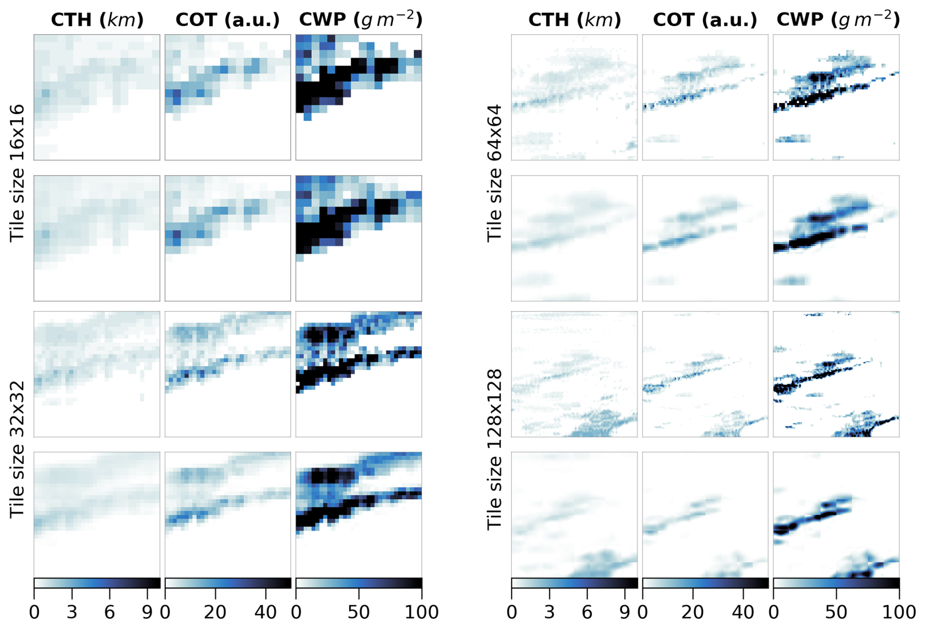
Figure B3 Input tiles (first and third rows) and corresponding reconstructions (second and fourth rows) for vision transformers trained on the relevant input tile sizes of 16, 32, 64 and 128.

B4 Spatial generalisation

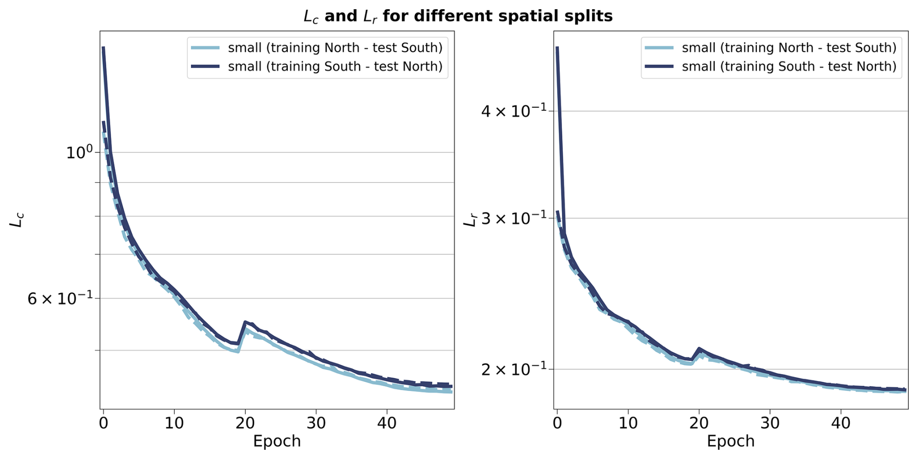
Figure B4 Training (full lines) and validation (dashed lines) metrics for the contrastive (left) and reconstruction (right) losses for vision transformers trained on samples from the Northern or Southern hemispheres.

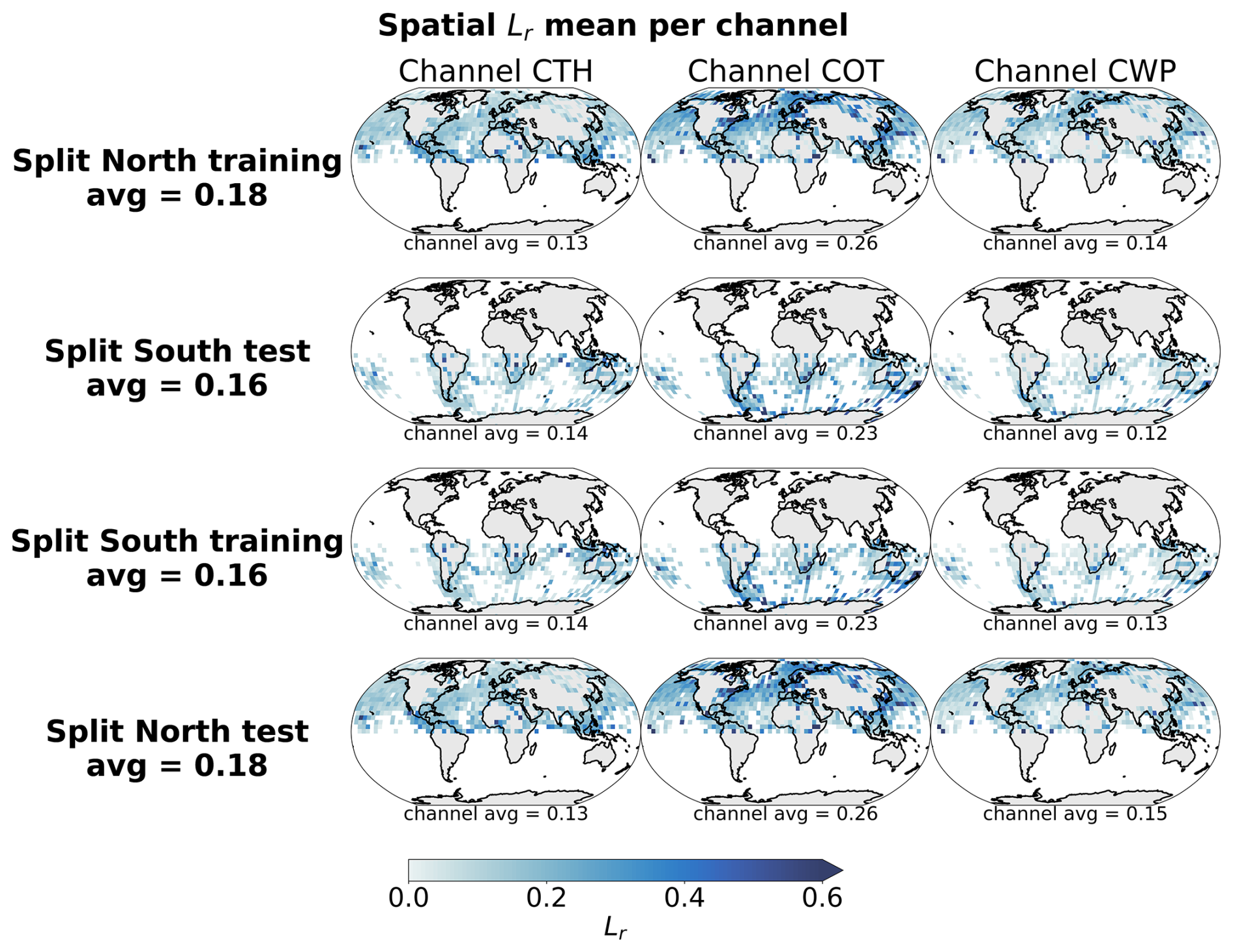
Figure B5 Spatial distributions of the mean channel reconstruction errors for the Northern and Southern hemispheres colocated samples. The first two rows correspond to the model trained on the samples from the Northern hemisphere and the last two rows to the model trained on the samples from the Southern hemisphere.

Appendix C: Cloud type classification for 10 types

Table C1 Classification metrics on the test set in the case of 10 cloud types. The metrics noted with a * are referring to their macro-averaged estimate. The baseline CNN/RF refers to the CNN backbone introduced in Lenhardt et al. (2024a).

The method on which the rest of the study is based is highlighted in bold.

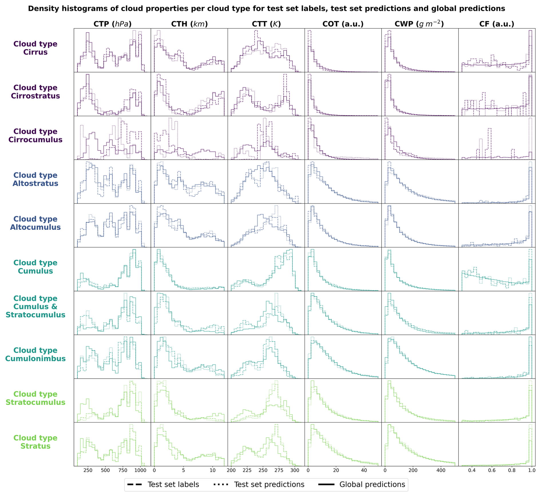
Figure C1 Density histograms of cloud properties for each cloud type from cirrus, cirrostratus, cirrocumulus, altostratus, altocumulus, cumulus, cumulus and stratocumulus, cumulonimbus, stratocumulus, stratus.

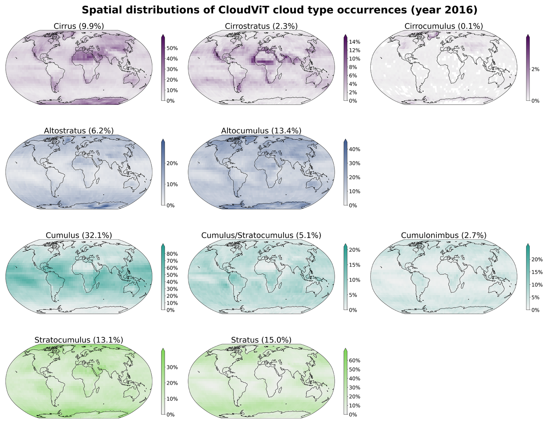
Figure C2 Spatial distributions of the CloudViT cloud type occurrences (cloud types cirrus, cirrostratus, cirrocumulus, altostratus, altocumulus, cumulus, cumulus and stratocumulus, cumulonimbus, stratocumulus, stratus) for MYD06 granules for the year 2016 aggregated on a 1° regular grid.

Appendix D: Exploring the technical feasibility of the application to a global storm-resolving model simulation

As a proof of concept and for probing the potential applicability of methods similar to CloudViT, we technically explore how to investigate the cloud type representation in general circulation model (GCM) outputs. We build on a new generation of GCMs at kilometre resolution, namely the ICON-Sapphire (Hohenegger et al., 2023). As the resolution of the simulation increases, some processes like deep convection can be directly resolved instead of parameterized. Hence, building diagnostics about cloud representation is of importance to help evaluate the simulations. In particular, we use the simulation run by the Max Planck Institute for Meteorology (MPI-M) for the period between the 5 and 12 December 1972, aiming at recreating the Blue Marble picture made during the Apollo 17 mission on the 7 December. Here we only use the complete outputs provided for the 11 December. The grid used contains 335 544 320 grid points at each level in the atmosphere (R02B11 grid), and outputs are provided every 30 min during the simulation for the atmospheric quantities of interest, resulting in overall 48 time steps. As the effective horizontal resolution of the model simulation and the MODIS data are on similar scales, we can technically effectively apply CloudViT on the model outputs. From the model outputs, we derive the cloud properties necessary for the method introduced in this study.

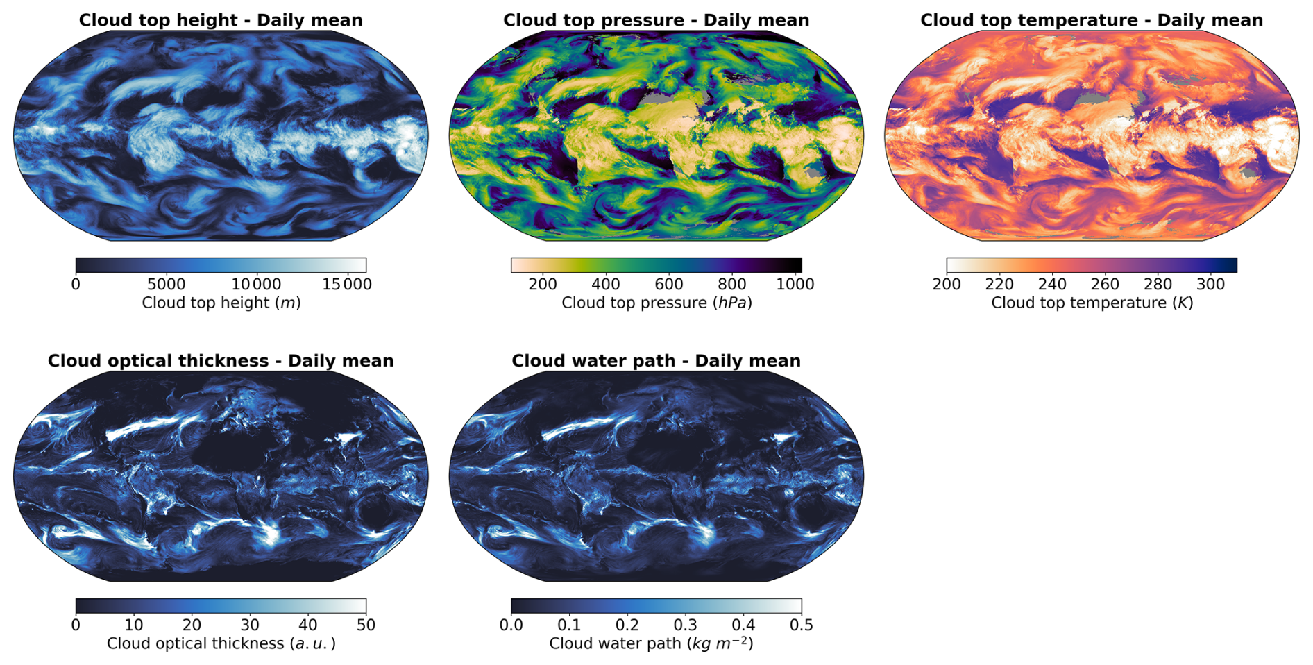
Figure D1 Daily averages of cloud top height, cloud top pressure, cloud top temperature, cloud optical thickness and cloud water path for the 11 December 1972 from the ICON-Sapphire Apollo 17 simulation.

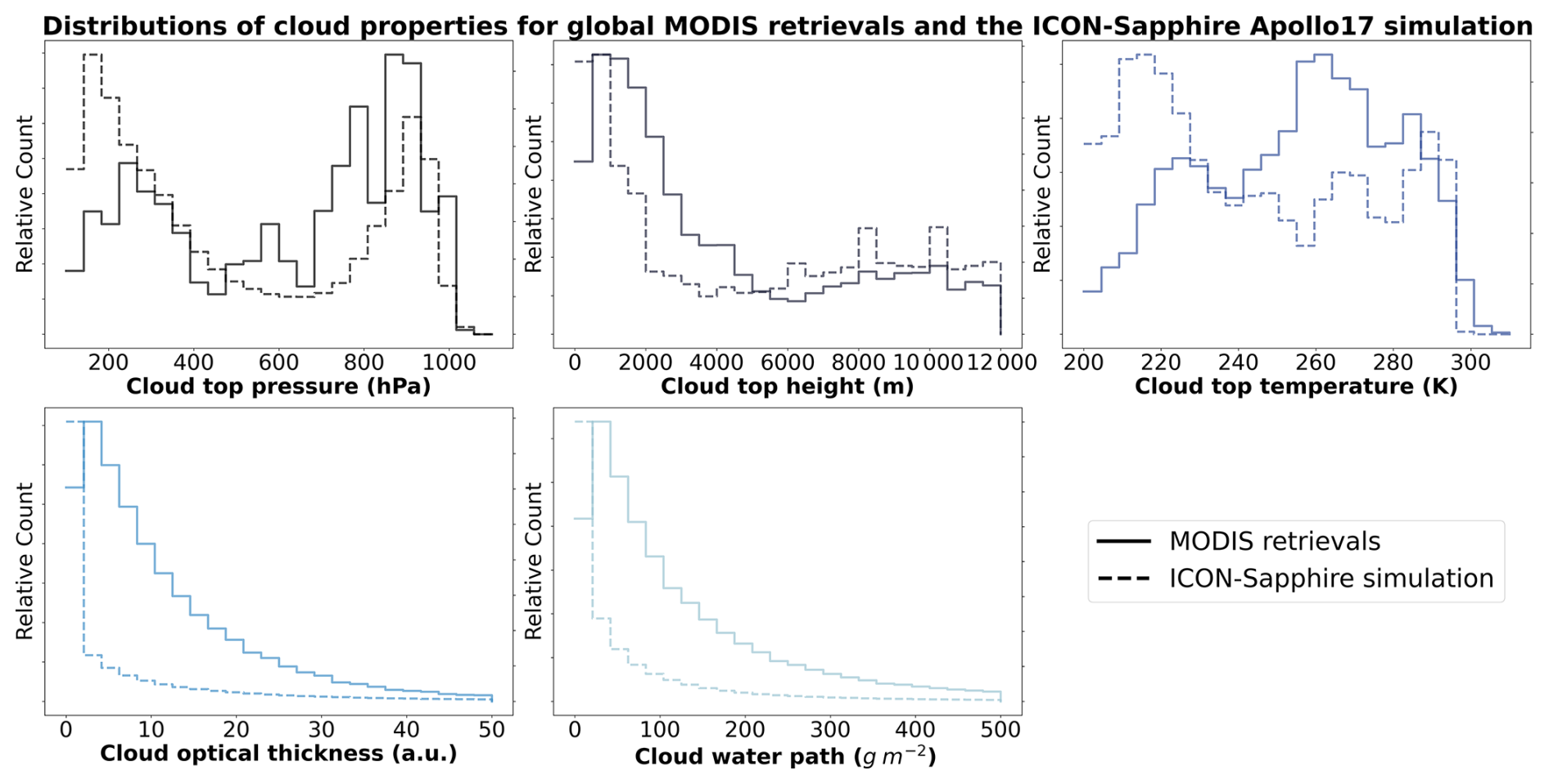
Figure D2 Distribution of cloud top pressure, cloud top height, cloud top temperature, cloud optical thickness and cloud water path for MODIS AQUA retrievals and the ICON-Sapphire Apollo 17 simulation.

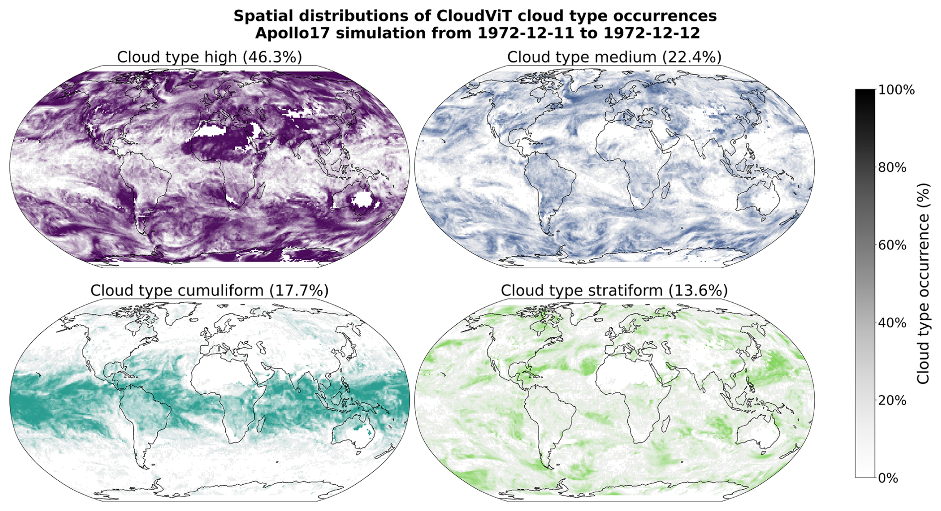
Figure D3 Spatial distributions of the CloudViT cloud type occurrences (cloud types high, medium, cumuliform, stratiform) for the ICON-Sapphire Apollo 17 simulation of 11 December 1972 aggregated on a 1° regular grid.

In order to compute the different cloud properties used in our method (Table 1), we use the available atmospheric outputs from the model simulation. The simulation was made using the ICON-2.6.6-rc version in R02B11 grid resolution with 90 vertical levels in the atmosphere (335 544 320 grid points per level) and 128 vertical levels in the ocean (237 102 291 surface grid points). Observed aerosols and greenhouse gas concentrations of December 1972 were used for the atmosphere. The cloud top quantities are retrieved by defining the top-most level where the liquid water content (variable name clw) or the ice content (variable name cli) are above a predefined threshold of 1 mg kg⁻¹. This threshold relates to particles of sizes of at least a few micrometres which is similar to what the sensors on the MODIS AQUA instrument are able to retrieve. Using 3D outputs of atmospheric quantities like temperature (variable name ta) and pressure (variable name pfull), we derive the cloud top properties also present in the MODIS MOD/MYD06 level 2 cloud properties product. The CTH is derived using the altitude in the corresponding vertical level in the grid. Secondly, the CWP is computed by summing the vertically integrated cloud liquid water path (variable name cllvi) and cloud ice path (variable name clivi) which are already provided as simulation outputs. Lastly, we computed the COT by vertically summing the layer-wise COT computed from the following equation, detailed in Carslaw (2022), Eq. (12.49) (Chapter 12.3, page 515):

$$\begin{array}{}\text{(D1)}& \begin{array}{rl}{\mathit{\tau }}_{\mathrm{c}}& ={\displaystyle \frac{\mathrm{9}}{\mathrm{5}}}{\left({\displaystyle \frac{\mathrm{4}\mathit{\pi }}{\mathrm{3}\sqrt{\mathrm{2}}}}\right)}^{\mathrm{1}/\mathrm{3}}{\mathit{\rho }}_{\mathrm{w}}^{-\mathrm{2}/\mathrm{3}}(k{N}_{\mathrm{d}}{)}^{\mathrm{1}/\mathrm{3}}{c}_{\mathrm{w}}^{-\mathrm{1}/\mathrm{6}}{L}^{\mathrm{5}/\mathrm{6}}\\ & =\mathrm{0.2303}k{g}^{-\mathrm{5}/\mathrm{6}}{m}^{\mathrm{8}/\mathrm{3}}(k{N}_{\mathrm{d}}{)}^{\mathrm{1}/\mathrm{3}}{L}^{\mathrm{5}/\mathrm{6}}\end{array}\end{array}$$

where $L=clw\cdot {\mathit{\rho }}_{\text{air}}\cdot \mathit{\delta }z$ the layer liquid water path, ρ_w=1000 kg m⁻³ density of water, k=1 a factor to account for the width of the droplet size distribution, $c_{\mathrm{w}}=\mathrm{2}{e}^{-\mathrm{6}}$ kg m⁻⁴ the adiabatic condensation rate and N_d the vertical droplet number defined in the simulation by the ECHAM6 parameterization (Eq. 6; Stevens et al., 2013). However, the standardisation of the input cloud properties for the vision transformer model is still done based on statistics computed on MODIS data which could induce a bias in the latent representations and subsequently on the predictions. Extending the method to other datasets like this GCM simulation thus requires careful investigation that the cloud properties lie in the same range or display similar distributions.

For each 30 min time step, we proceed to sample tiles, regularly spaced, to reach global coverage of cloud type estimates. Figure D3 displays the daily averaged occurrence of the cloud type predictions on a 1° regular grid for the 4 cloud types, the equivalent for 10 cloud types is presented in Fig. D4. However, due to the time period covered by the simulation, no global data record for cloud types can be used to evaluate the representation of cloud types by the ICON-Sapphire through the CloudViT method. A thorough analysis would be feasible for simulations covering a time period for which climate data records of cloud types are available, for example the ISCCP H-series climate data record (Young et al., 2018) which starts in 1983. The aim here is rather to present as a proof of concept the transfer of such a method to model data outputs. A large proportion of the predicted clouds belong to the high cloud type, hinting at the difference in sensitivity to clouds retrieved in the climate model data compared to the MODIS retrievals or the mismatch in the training process of CloudViT, high clouds being underrepresented and their corresponding classification metrics lower than for some other cloud types. However, increasing the cloud ice content threshold by an order of magnitude greatly decreases the amount of thin, high and cold clouds in the simulation dataset. This aspect would need further tuning through comparison with remote sensing retrievals which are not available for this particular simulated period. An important aspect to factor in is that the classification model was only trained on daytime satellite observations as the optical cloud properties necessary are only available then. Thus, results on nighttime cloud retrievals which is the case for some of the predictions produced from the presented simulation might need more meticulous evaluation. Even though it is a limiting factor in the case of the satellite dataset we are using, the simulation outputs provide us with the required variables across all timesteps.

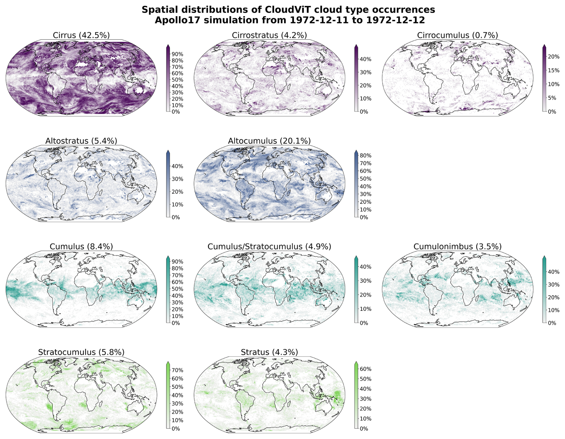
Figure D4 Spatial distribution of the CloudViT cloud type occurrences (cloud types cirrus, cirrostratus, cirrocumulus, altostratus, altocumulus, cumulus, cumulus and stratocumulus, cumulonimbus, stratocumulus, stratus) for the ICON-Sapphire Apollo 17 simulation of 11 December 1972 aggregated on a 1° regular grid.