A detailed comparison of the Dutch emission inventory with satellite-derived NO_x emissions

Nitrogen oxides are one of the most important air pollutants with a large impact on human health. Their emissions are monitored by national emission inventories that are the basis for emission related policies. Because of their large impact on policies these emission data should ideally be verified against independent data, such as emission estimates derived from atmospheric observations. Here, we present a detailed comparison of NO_x emissions from the Dutch national emission inventory with completely independent emission data derived with the DECSO algorithm from satellite observations by TROPOMI on board of sentinel 5-P. This is enabled by the introduction of a new high-resolution DECSO version DECSO-HR 6.5. We find good agreement in overall emission levels, the spatial emission pattern, the 5-year emission trend, and regional emissions, with deviations in the yearly variation of emissions and at large point sources. Our results demonstrate the robustness of the national inventory and the satellite-derived emissions. This approach might serve as a use-case for the adoption of similar methods in other countries.

1 Introduction

Nitrogen oxides (NO_x) are among the most important air pollutants. Besides their negative effect on human health, they also impact the nitrogen cycle leading to eutrophication and acidification and contribute to climate change. For these reasons, the European Union imposes strict regulations on nitrogen oxide emissions. As part of the emission monitoring, national emissions of nitrogen oxides have to be reported as part of the Convention on Long-Range Transboundary Air Pollution (CLRTAP; EEA, 2024b) and the National Emission Ceiling Directive (NECD; EEA, 2024a) of the European Union. To assess if countries adhere to their emission targets, detailed bottom-up emission inventories are compiled by each Member State. Although this legislature has been successful in reducing European NO_x emissions, the Member States of the European Union combined still emitted 1640 kt NO_x (expressed as N) in 2022 (according to NEC reporting; EEA, 2024b), of which the Netherlands, as a small, but industrialized and densely populated Member State, are responsible for 58 kt (N) (Staats et al., 2025). Although the Netherlands are expected to hit their 2023 NEC emission reduction targets, NO_x emissions contribute significantly to the so-called nitrogen crisis in the Netherlands which centers around nitrogen deposition in protected nature areas, of which about 30 % is related to NO_x emissions (Hoogerbrugge et al., 2023). Therefore, monitoring and reduction of NO_x emissions remains crucial. Since the national emission inventories are the basis for policies on emissions and air quality, they are very impactful and would ideally be verified against independent data.

Besides the national inventories, there also exist global and regional emission inventories, for example the Emissions Database for Global Atmospheric Research (EDGAR: Olivier et al., 2021) or the emission inventories provided by the Copernicus Atmospheric Monitoring System (CAMS; Kuenen et al., 2022; Soulie et al., 2024). However, these inventories usually rely on the same or similar methods and data as the national inventories. A truly independent method to assess emissions of air pollutants are so called top-down methods based on atmospheric observations. In these approaches, the concentrations of air pollutants in the atmosphere are derived from observations by ground-based stations or satellites, which are then used to infer emissions. There exist different methods to solve this inverse problem, like the divergence method (Beirle et al., 2023), plume fitting (Beirle et al., 2011) and inverse modelling (Miyazaki et al., 2012; Stavrakou et al., 2008). An established inverse modelling algorithm to derive emissions using satellite observations is DECSO (Daily Emissions Constrained by Satellite Observations) (Mijling and van der A, 2012). This algorithm has been widely used for a variety of different regions and gases and has been shown to show good correlation with national inventory emissions of NO_x and NH₃ for European countries (Ding et al., 2024; van der A et al., 2024). DECSO has also been applied to study the effect of COVID on NO_x emissions in China (Ding et al., 2020) and the emissions of large cities and point sources (van der A et al., 2024).

In principle, as an independent method, inverse modelling provides the ideal data for validation or verification of bottom-up emission inventories: an independent emission dataset that the inventory can be compared against. Operational national verification schemes using inverse modelling have been established for different greenhouse gases for a number of countries, for example Switzerland (FOEN, 2025) and the UK (Brown et al., 2025). However, there are so far fewer comparable verification activities for air pollutants such as nitrogen oxides. Studies of satellite-based NO_x emission verification on a local and national scale were performed for Germany (Dammers et al., 2023) and the USA (Li et al., 2021; Ma et al., 2025). Few Informative Inventory Reports on air pollutants include a comparison with satellite-derived emissions of air pollutants for verification purposes, among them Germany (UBA, 2025) and the Netherlands (Staats et al., 2025). While the DECSO algorithm has been widely used for a variety of different regions and gases (Ding et al., 2024; van der A et al., 2024), it has not yet been thoroughly applied for emission verification on a national and subnational scale. One challenge in using inverse modelling for emission verification in particular for smaller countries like the Netherlands is the relatively coarse resolution for most inverse modelling setups, which is limited by computational cost and the resolution of satellite observations and meteorological parameters. The resolution is especially crucial for analysing emissions on a local scale, e.g. for individual cities or industrial installations, and for attribution of emissions to different processes.

In this paper, we present a detailed comparison of the Dutch national emission inventory and emission data generated by DECSO with the goal to verify the national emission inventory that forms the basis for emission policies. This was enabled by the development of a high resolution version of DECSO-HR, which improved the resolution to 0.05°, close to the resolution of the used TROPOMI observations, and a new version DECSO 6.5 is introduced. NO_x emissions for a focus region centred on the Netherlands were derived from TROPOMI observations and were compared to the official national emission inventory with regards to overall emission levels, the spatial distribution and emission trends. We also explore the possibilities for emission verification on provincial and municipal levels. This detailed comparison for the Netherlands might serve as a use-case for other countries and forms a starting point for a new NO_x emission verification and monitoring regime in the Netherlands.

2 Methods and data sources

2.1 DECSO

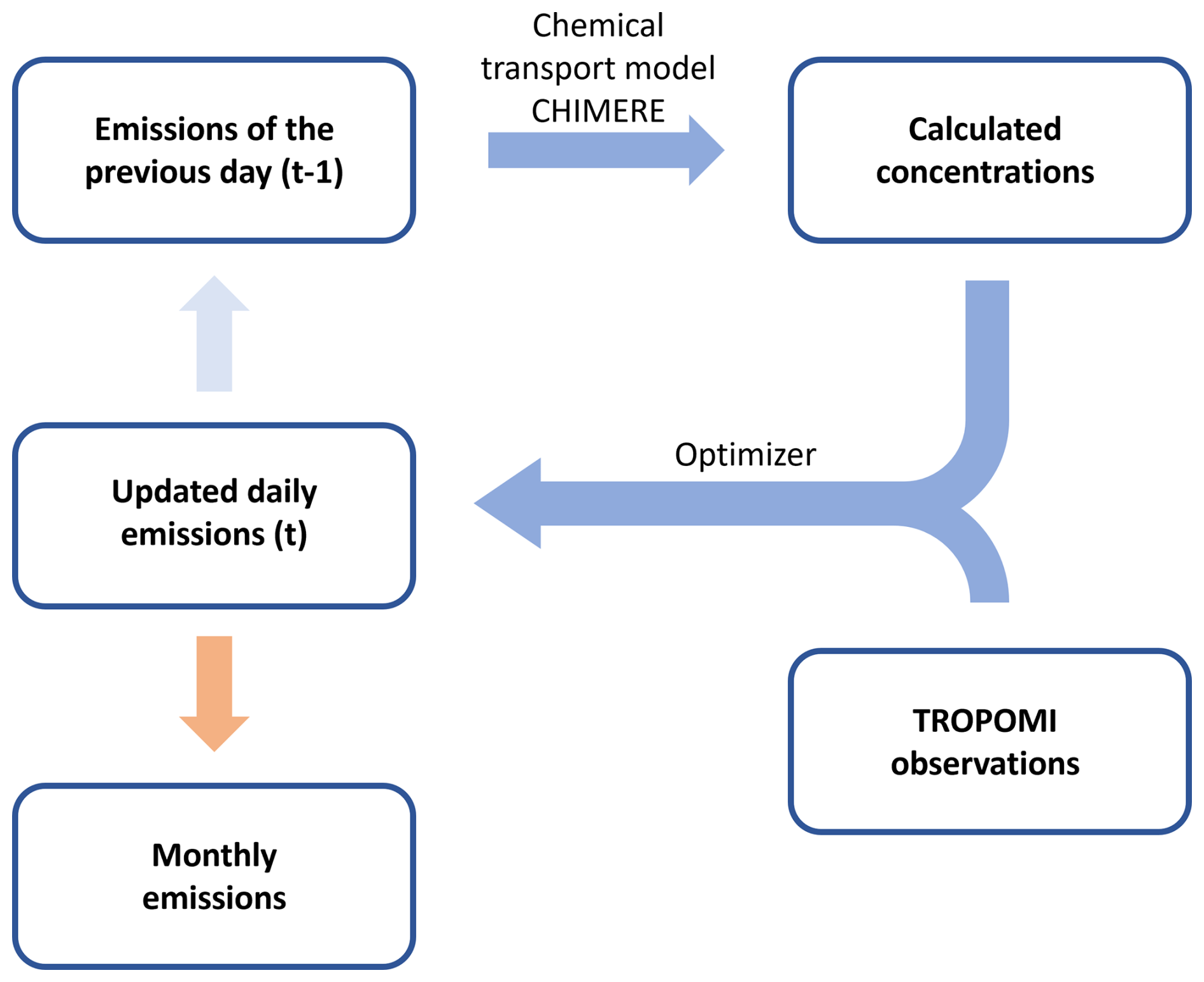
The inversion algorithm DECSO (Daily Emissions Constrained by Satellite Observations) has been developed at KNMI for the purpose of deriving emissions for short-lived gases (Mijling and van der A, 2012, Fig. 1). DECSO is using a Kalman Filter implementation for assimilating emissions, which includes the following steps: the sensitivity matrix (or Jacobian) to describe the relation between gridded emissions and satellite observations is derived using an ensemble of trajectories calculations with an estimated effective lifetime of the trace gas. The satellite observations are compared to the concentrations modelled by the chemical transport model (CTM) CHIMERE v2020r3 (Menut et al., 2021). The difference between model and observations is used to adapt the emissions within the data assimilation scheme. Since these adaptations are based on additions or subtractions and no scaling is involved, emerging or disappearing emission sources are also detected. Note that the a-priori emissions are not from an external inventory but based on the emissions of the previous day which are updated based on the mismatch between observations and forecast with a spin-up period of 200 days before the emission results are used. After this period any effect of the day one a-priori emissions is gone due to the additive assimilation scheme. As prior emissions for day 1, HTAP v3 was used (Crippa et al., 2023). DECSO is currently designed to estimate NO_x and/or NH₃ emissions. Detailed information on the inversion method can be found in Mijling and van der A (2012).

Figure 1 Scheme illustrating the DECSO algorithm.

For deriving NO_x emissions, we use NO₂ observations of the TROPOMI instrument on board Sentinel 5P (van Geffen et al., 2022). Only observations with a cloud radiance fraction of less than 50 % (this corresponds to a cloud fraction of about 20 %) are selected for input to DECSO, which is about 50 % of all observations. The precision of the derived NO_x emissions is estimated as 8 % for annual emissions and 25 % for monthly emissions (van der A et al., 2024).

The version we used at the start of this study is version 6.4. It is actually the same code as version 6.3, published in van der A et al. (2024), Ding et al. (2024), and Lin et al. (2024), except that the vertical emission profiles for industrial sources used in the CTM were updated following the analyses of Bieser et al. (2011). In this study we focused on the Netherlands (50–54° N, 2–9° E), which is a relatively small country, and a higher resolution emission grid of NO_x emissions was required for a detailed intercomparison. To facilitate such an intercomparison a new high-resolution version of DECSO was developed named DECSO-HR. While the original version of DECSO had a 0.1° resolution, the newly developed DECSO-HR focussed on the Netherlands at a 0.05° resolution, comparable to the resolution of the TROPOMI observations, which are 3.5×5.5 km at nadir. Besides small changes concerning the harmonization of the parameters related to spatial and temporal resolution (for example a smaller time step and a shorter distance for the trajectory calculations) the main difference between the standard DECSO and DECSO-HR is their input. The TROPOMI observations used for DECSO-HR are more numerous and have higher uncertainties than the super-observations (area-weighted means of cloud-free TROPOMI observations, see below) used in DECSO. On the other hand, the direct observations are better spatial matched with the emissions. Together with additional developments of the algorithm to improve its quality, this has led to the release of version 6.5. Some of these points of improvement were notably revealed by the comparison to the Dutch emission inventory.

The changes from 6.4 to 6.5 included some minor corrections such as including the seasonal cycle of VOCs, adapted vertical emission profiles for ship emissions and an error correction for high concentrations to avoid the assimilation to favour the majority of low emissions in the region. The main changes that will be discussed below were related to the use of a new superobservation code, a correction of NO₂ observations in winter, and a fixed lifetime specifically for the high-resolution version.

DECSO is using superobservations, which are area-weighted means of cloud-free TROPOMI observations over the model grid cells. The software to construct these superobservations has been replaced by the software of Rijsdijk et al. (2025), which provides a more realistic description of the superobservation uncertainties. At the same time, the observations of the tropospheric column till 500 hPa are calculated. However, these superobservations are not used for the HR-version of DECSO because the model grid and the TROPOMI resolution are almost equal and the advantage of superobservations disappears. For the HR version the tropospheric column of NO₂ till 500 hPa is used directly as input to DECSO. Another change for the HR-version of DECSO is that the effective lifetime of NO_x is no longer derived locally but fixed to 3 h. This significantly improves the calculation time at the cost of slightly slower convergence speed to match the emissions to the observations. This lifetime is only part of the trajectory calculation within DECSO in addition to the intrinsic NO_x lifetime of the CHIMERE model. While the former lifetime determines the convergence speed of the emission updates, the magnitudes of the emissions are mainly impacted by the intrinsic NO_x lifetime of the CHIMERE model, since the derived daily emissions are based on minimizing the difference between the model output and the satellite observations. The difference of the final monthly emissions with and without fixed lifetime in the DECSO trajectory calculation is negligible.

During this study we noticed the TROPOMI NO₂ observations were unrealistically low or even negative during days in the winter with strong wind coming from northerly to westerly directions. This was corrected by using a reference sector above a relatively clean area over the North Sea to determine the bias between the CTM of DECSO and the NO₂ retrievals. The effect of this correction can also be seen in Fig. 4b.

Although DECSO provides additional information on anthropogenic emission and soil emissions (Lin et al., 2024), in this paper only the total NO_x emissions are analysed.

2.2 Dutch emission inventory

The national Dutch emission inventory (in Dutch Emissieregistratie) reports emissions for 375 different substances towards air and water, including the most important air pollutants like NO_x, SO_x and particulate matter and all greenhouse gases. It also compiles the Informative Inventory Report about air pollutant emissions (Staats et al., 2025) which is annually published to fulfil obligations under CLRTAP and NECD. The methods used to calculate emissions are detailed in the yearly method reports of each sector (Honig et al., 2025; van der Zee et al., 2025; Visschedijk et al., 2025; Witt et al., 2025). Most data from the emission inventory, including spatial gridded data and emissions per province and municipality for this analysis were downloaded from https://www.emissieregistratie.nl/data (last access: 19 March 2026). Some additional data like the large point source data were produced by the emission inventory on special request.

2.3 Data analysis

To calculate national, provincial and municipal Dutch emissions from the satellite data grid cells within the Netherlands, excluding the North Sea, were selected using the exactextractr package in R (Baston, 2025). For grid cells partially in an area, the emissions were distributed based on the share of the grid cell within the Netherlands. Regridding of inventory data to the DECSO resolution was carried out using the resample function of the terra package in R by calculating mean fluxes (Hijmans, 2025). Monthly inventory emissions were calculated by mapping the emissions from the emission inventory to GNFR sectors in order to use temporal emission profiles from the CAMS-TEMPO v4.1 data set (Guevara et al., 2021). The majority of NO_x emissions in L_AgriOther in the Netherlands is from application of manure to agricultural soils. However, the profile for NO_x emissions from L_AgriOther in CAMS-TEMPO is based on burning of agricultural waste, a practice not legal in the Netherlands. Therefore, the profile for NH₃ was used instead.

2.4 Other data sources

For additional emission data outside the Netherlands CAMS-REG-ANT v8.1 was used (Kuenen et al., 2022), which utilizes the reported national emissions and uses a consistent method for gridding of the emissions. Monthly emissions were estimated using CAMS-TEMPO v4.1 (Guevara et al., 2021). Official national, provincial and municipal borders of the Netherlands were downloaded from PDOK (2024). Information on the Dutch road network were downloaded from RWS (2024).

2.5 Uncertainties

The uncertainty of the NO_x emissions quantified with DECSO at the scale of the Netherlands was previously quantified and estimated as 8 % (95 % confidence interval) (van der A et al., 2024). Additional uncertainties arise from the applied country mask, which have so far not been quantified. The uncertainty of the total Dutch NO_x emissions in the Dutch National Inventory was previously calculated with a Monte-Carlo analysis based on the estimated uncertainties of individual emission sources and was found to be 19 % (95 % confidence interval) (Staats et al., 2025). Uncertainties in the spatial or temporal distribution of the Dutch National Inventory have so far not been analysed.

3 Results and discussion

3.1 Inventory emissions and satellite observations show qualitative agreement

Figure 2 shows a comparison of emissions maps for the year 2019 as reported by the Dutch national emission inventory and as derived from satellite observations analysed with the DECSO algorithm (total emissions) using the original DECSO 6.4.1 at 0.1° resolution and the newly introduced DECSO-HR 6.5 with a resolution of 0.05°. As the Dutch national emission inventory covers only the Netherlands, emissions for neighbouring countries were added from CAMS-REG-ANT (Kuenen et al., 2022). To allow for an easier visual comparison, the inventory dataset is also shown interpolated to the DECSO-HR resolution of 0.05°.

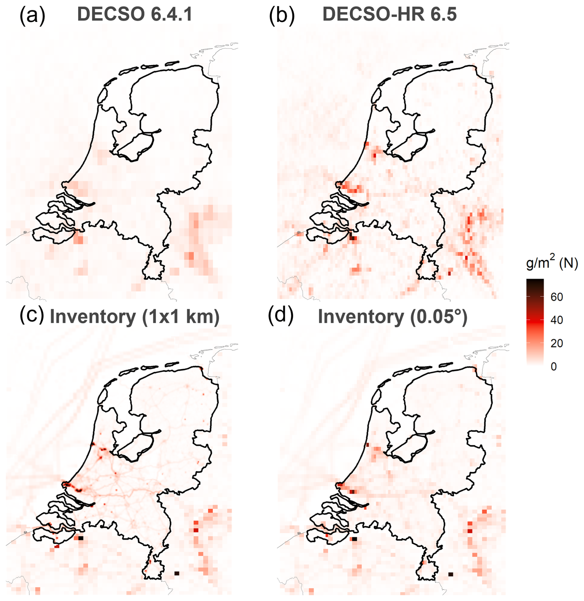
Figure 2 Maps of annual NO_x emissions for 2019 according to satellite observations analysed with (a) DECSO 6.4.1 (0.1° resolution), (b) DECSO-HR (0.05° resolution), (c) the Dutch national emission inventory on 1 km resolution and (d) interpolated to 0.05°. Inventory emissions outside the Netherlands are added from CAMS-REG-ANT (at a resolution of 0.05°×0.1°). To allow better visualization fluxes in (c) were limited to 75 g m⁻².

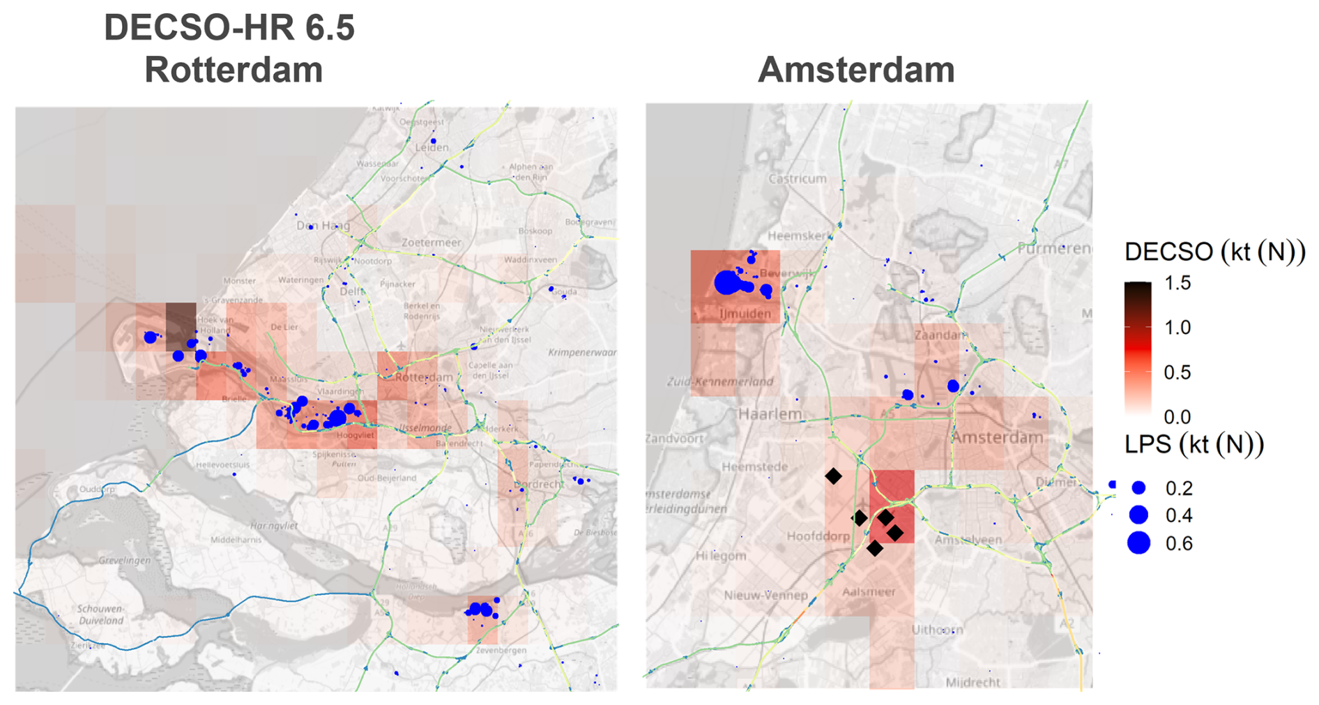
Figure 3 Zoom-ins on the urban and industrial areas in and around Rotterdam and Amsterdam. Blue circles mark large point sources (LPS), highways are shown as lines with the colour indicating the number of lanes (increasing from blue to red), black diamonds mark the runways of Schiphol airport. Map data © OpenStreetMap contributors 2025. Distributed under the Open Data Commons Open Database License (ODbL) v1.0.

First, comparing DECSO 6.4.1 and DECSO-HR 6.5, the increased resolution clearly provides additional detail. While large emission hotspots within and outside the Netherlands, like Amsterdam, Rotterdam, Antwerp and the Rhine–Ruhr area can be recognized in both data as reported earlier (van der A et al., 2024), the improved resolution of DECSO-HR 6.5 reveals additional valuable details, like distinguishing the emissions from Amsterdam and the industrial complexes in IJmuiden (in the North-West of the Netherlands, see also Fig. 3) or resolving individual emission hotspots within the German Rhine–Ruhr area (in the South-East of the domain).

Next, the comparison between DECSO-HR 6.5 (Fig. 2b) and the national emission inventory (Fig. 2c and d) directly shows the good spatial agreement between these two independent emission datasets. Both emission maps clearly show the urban emission hotspots of Amsterdam, Rotterdam and Utrecht in the Western part of the Netherlands. On the inventory emission maps one can also clearly recognize the network of high-ways and rivers (used for inland navigation) in the Netherlands. These features are also indicated in the DECSO-HR 6.5 emission map (Fig. 2b), while not being recognizable in DECSO 6.4.1. Interestingly, while not all shipping routes on the North Sea in the inventory dataset are resolved in DECSO-HR 6.5, the main shipping routes towards Rotterdam and Antwerp are still captured.

Zooming closer on the biggest cities Rotterdam and Den Haag (Fig. 3, left panel) and Amsterdam (Fig. 3, right panel) and their surrounding industrial areas in DECSO-HR 6.5, one can clearly see the good correlation between registered point sources (blue circles) and the satellite emissions estimates. Also Schiphol airport (runways marked with black diamonds) is clearly visible in the satellite data set. Interestingly, the highway network around these cities (indicated in rainbow colors) is not visible in the DECSO-HR emission maps despite road traffic being a major source of NO_x as will be discussed further below.

3.2 Comparison of annual and monthly national total emissions

Next, for a quantitative comparison of the emission inventory with satellite-based emission estimates, we compare the timeseries of total national emissions from 2019 to 2023 for DECSO 6.4.1 and DECSO-HR 6.5 as shown in Fig. 4. To calculate national total emissions from the DECSO datasets, grid cells within the Netherlands, excluding the Dutch part of the North Sea, were added up. For the time span investigated here, the national inventory reported monotonously decreasing emissions from 76 kt (N) in 2019 to 61 kt (N) in 2023 (Staats et al., 2025). In comparison, DECSO 6.4.1, the latest version of DECSO when this work started, reported only 44 kt (N) in 2019. By contrast, DECSO-HR 6.5 was much closer to the inventory with 68 kt (N) in 2019 and agrees with the inventory within the uncertainty range for all years except for 2021.

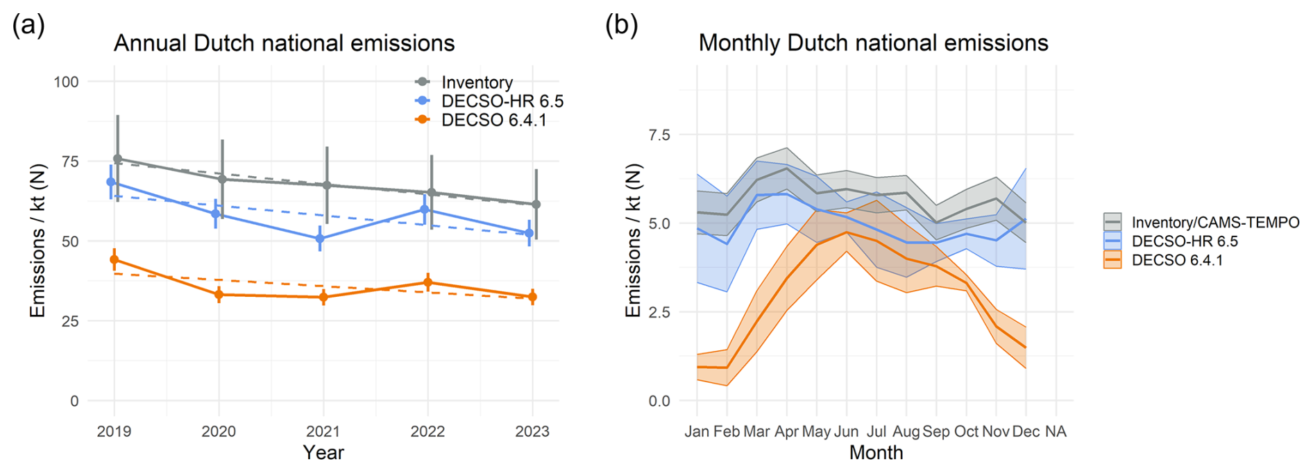
Figure 4 (a) Total annual Dutch emissions from 2019 to 2023 with trend lines shown as dashed lines and (b) mean monthly emissions (averaged from 2019 to 2023) according to the Dutch national emission inventory (combined with CAMS-TEMPO), DECSO 6.4.1 and DECSO-HR 6.5. Error bars and the shaded area both show the 95 % confidence interval.

There is, however, a notably difference in the inter-annual variation between the different emission data: While the inventory emissions decline monotonously from 2019 to 2023, DECSO-HR 6.5 reports a minimum in 2021 and an increase from 2021 to 2022. This might be due to the effects of the COVID pandemic not being captured accurately by the emission inventory. While changes in the activity data, i.e. the economic activity, were presumably accurately captured by national statistics, there are also possible, less obvious effects on the emission factors, for example lower emission factors from road traffic as traffic was less congested. While there were attempts to also include these effects, these certainly lead to higher uncertainties in the inventory emissions that are so far not well understood. These data thus might imply that emission reduction during the pandemic was underestimated by the national inventory, but other explanations are also feasible, for example meteorological conditions.

Despite these differences, fitting a trendline to the emissions from both DECSO-HR 6.5 and the inventory (dashed line in Fig. 4a) led to similar emission trends with a yearly reduction of 3.1 kt (N) for DECSO-HR 6.5 and 3.3 kt (N) for the inventory, showing that emission trends on intermediate timescales of several years agree between the two data sets.

Besides the inter-annual emission trend, we also compared the intra-annual variation of emissions. Therefore, mean monthly emissions from satellite observations were compared to monthly inventory emissions (Fig. 4b). As the Dutch national inventory only produces annual emissions, monthly inventory emissions were estimated by distributing the inventory emissions per GNFR sector using the CAMS-TEMPO temporal profiles (Guevara et al., 2021). This comparison revealed large differences in the temporal profiles. While the inventory emissions were roughly constant throughout the year with higher emissions from stationary combustion and road transport in winter being compensated by higher emissions from agriculture and non-road mobile machinery in summer, DECSO 6.4.1 shows a strong minimum of emissions in winter, with emissions in January being just 20 % of emissions in June (Fig. 4b). This deviation in winter also explains the large deviation in yearly emissions between the inventory and DECSO 6.4.1 in Fig. 4a. The low DECSO emissions in winter were caused by a bias in the TROPOMI NO₂ retrievals for observations with a strong north-western wind in the winter when NO₂ observations were close to zero or even negative. Correction of this bias in DECSO-HR 6.5 (see Sect. 2.1) therefore remedied this winterly mismatch. Monthly emissions according to DECSO-HR 6.5 agree within the uncertainty range with inventory emissions.

Taken together, the improvements introduced with DECSO-HR 6.5 not only provided more spatial information but also improved the match to inventory emissions.

3.3 Quantitative comparison of spatially explicit emissions

After analysing the temporal match of the emission datasets, we next considered their spatial correlation as shown in Fig. 5. Figure 5a shows a difference map for 2019 between the national inventory and DECSO-HR 6.5. In general, this map confirms the good agreement between the two data sets. There are no systematic deviations or biases apparent on a national scale and deviations could only be observed in the Amsterdam/IJmuiden and Rotterdam areas (Fig. 5b). In these areas, DECSO yields overall lower emissions than reported in the inventory. Interestingly, it appears that in these areas there might be an alternating pattern of positive and negative deviations, which will be further discussed below.

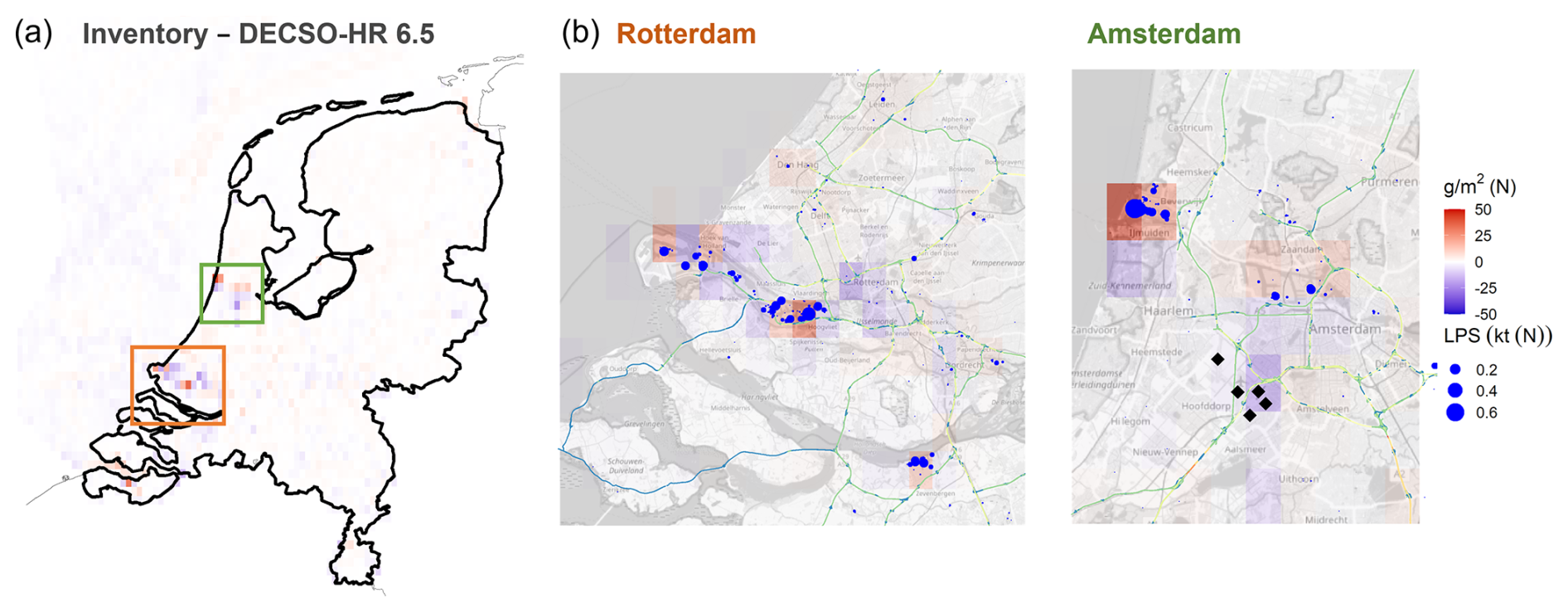
Figure 5 (a) Difference between the annual NO_x emissions according the inventory and DECSO-HR 6.5 per grid cell for 2019. Red colors indicate that the inventory has larger emissions, blue that DECSO results are higher. (b) Zoom-ins on the industrial areas in and around Amsterdam and Rotterdam. Blue circles mark point sources, highways are shown as lines with the color indicating the number of lanes (increasing from blue to red), black diamonds mark the runways of Schiphol airport. Map data © OpenStreetMap contributors 2025. Distributed under the Open Data Commons Open Database License (ODbL) v1.0.

In the zoom-in views of urban areas, also highways and Schiphol airport are indicated as the transport sector is the main source of NO_x emissions in the Netherlands. Schiphol airport (with black diamond's indicating the runways) is clearly visible in the DECSO emission maps (Fig. 3). Considering also the difference maps (Fig. 5b), DECSO-HR 6.5 reports higher emissions than the national inventory over Schiphol airport. This might be caused by the national inventory only reporting emissions for the landing and take-off phase of the flights (LTO) up to 3000 ft (∼914 m) according to international agreements, thereby missing emissions above 3000 ft, which have been estimated at 4 kt (N) over the entire Netherlands (Witt et al., 2024) of which about 2/3 are related to air traffic at Amsterdam Schiphol airport. These emissions will in parts still contribute to satellite observations of column densities. The highway network on the other hand was not very apparent in the emission maps (Fig. 3) or the difference maps (Fig. 5b), indicating that as a diffuse source road traffic will be difficult to spatially isolate in the DECSO emissions.

As these two areas around Rotterdam and Amsterdam have large industrial sides and harbours and consequently high emissions, we hypothesized that the deviation between the two datasets was depending on the intensity of the fluxes. To further explore these deviations, emissions according to DECSO-HR 6.5 were plotted per grid cell as a function of the inventory emissions in that same grid cell (Fig. 6a), which revealed two different behaviours at low and high emissions. At low emissions (below roughly 0.25 kt (N), yellow shading) emissions per grid cells showed on average good correlation (dark blue circles), albeit with some scatter. At larger emissions (blue shading), however, the two datasets started to deviate, with the mean DECSO emissions moving further and further from the unity line. This can be seen even more clearly when considering the difference between the two datasets as a function of inventory emissions (Fig. 6b). The mean deviation was close to 0 at small emissions below 0.25 kt (N) (yellow shading) and started to increase at higher emissions (blue shading). It reached 0.5 kt (N) for grid cells with emissions around 1 kt (N), a deviation of almost 50 % for these highly-emitting grid cells. These deviations at high emissions had a large impact on the total estimated national emissions: Grid cells with an emission larger than 0.5 kt (N) in the emission inventory were responsible for 53 % of the observed deviation between inventory and satellite observations on a national scale in 2019, despite representing only 0.4 % of grid cells.

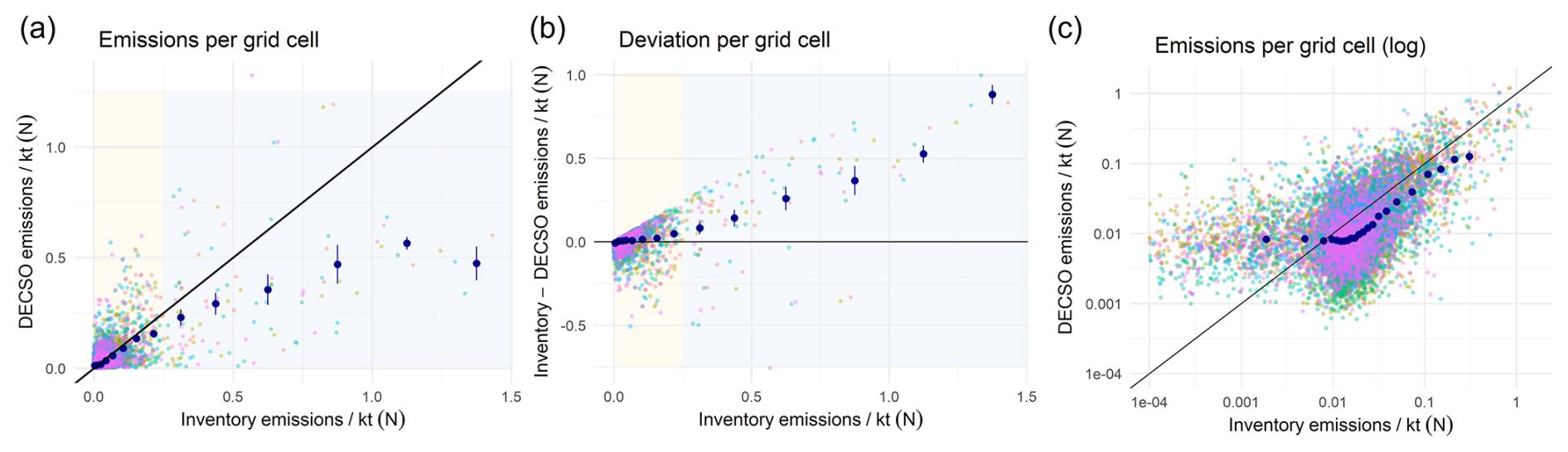
Figure 6 (a) Correlation between the two emission datasets per grid cell. The unity line is shown in black. (b) Difference between the two emission estimates per grid cell as a function of the emission of that grid cell according to the Dutch national emission inventory. (c) Same as (a) but on a log-log scale. Dark blue dots are the average of all grid cells over all years, error bars show standard errors, yellow and blue shadings mark the low and high emission behaviour, respectively.

This leads to the question where these large deviations are coming from, an underestimation by the satellite-derived emissions or an overestimation by the inventory. On the inventory side, these high-emission grid cells relate to areas of high industrial activity whose emissions are registered as large point sources. The quantity of these emissions is being reported by the companies themselves, according to standardized methods and controlled by local environmental authorities (Staats et al., 2025). That means that the location of these emission sources is precisely known leading to neglectable spatial uncertainty. On the other hand, while there are certainly uncertainties in the amount of emissions, there are no records of systematic overreporting of industrial emissions. Looking at satellite-derived emissions, a part of this deviation might be explained by the emissions from large point sources being wrongly allocated to neighbouring grid cells, in other words appearing smeared out over a larger area which might be caused by uncertainties in the wind fields. This would lead to an alternating pattern of over- and underestimated grid cells, as can indeed be seen in Fig. 5b. However, while this fits qualitatively, these alternating pixels do not compensate each other quantitively, meaning that even when adding these grid cells up DECSO reports lower emissions for highly emitting areas than the inventory. In absence of a known ground truth, more research and further independent assessments will be needed to fully understand these deviations.

Figure 6c shows the same data as Fig. 6a but plotted on a double-logarithmic scale in order to better assess grid cells with low emissions, which are dominated by diffuse sources. Here, again, different behaviours can be distinguished. At very low inventory emissions below 0.01 kt (N), the DECSO emissions reached a plateau at around 0.01 kt (N), which is presumably caused by NO_x emissions from soils. The overall contribution of these grid cells to the total emissions is very small with only 3 %, despite representing 22 % of all grid cells. Above 0.01 kt (N) the two data show a good correlation, however with a slight offset towards inventory emissions. This means that also in these low-emitting grid cells the inventory reports on average higher emissions than DECSO, albeit with a very small difference.

Taken together, a good spatial correlation between the two emission data sets was observed, with deviations at both ends of the emission range. Of these two deviations, however, the one at low emissions hat a negligible impact on overall emission levels, while the deviation at high emissions had a major impact.

3.4 Possibilities for emission verification from regional to municipal scale

The high resolution of the DECSO-HR algorithm of 0.05° (about 5 km in the Netherlands) becomes comparable to the size of cities, municipalities and provinces, which might allow comparison and verification of inventory emissions even on these smaller, local scales. This could potentially be very useful, not only for a better understanding of emission sources, but also because emissions at the local scales have a high relevance for policies.

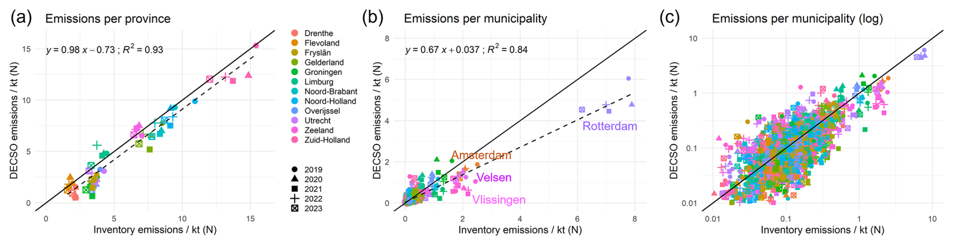
Figure 7 (a) Comparison of annual NO_x emissions according to DECSO-HR 6.5 and the Dutch national emission inventory (a) per province, (b) per municipality on a linear scale, and (c) per municipality on a double-logarithmic scale. Unity is shown as a solid line, while the dashed line represents a linear fit.

Here, we will evaluate these possibilities for the use-case of the Netherlands beginning on the scale of provinces (Fig. 7a), of which there exist 12 in the Netherlands, with populations ranging from 390 000 to 3 800 000 and land areas between 1400 and 5400 km². Comparing the emissions per province according to the inventory and according to DECSO-HR 6.5, we see good agreement between the two data sets. A linear fit revealed a slope of 0.89 with R² of 0.93. That means that a small bias remains, where also on a provincial level the emission inventory reports slightly higher emissions than DECSO-HR 6.5. However, the good correlation supports the possibilities of emission verification by satellite observations also on the regional scale.

Next, we zoom-in closer, looking at the scale of municipalities (in Dutch gemeenten), which can have a size as large as 523 km² and as small as 7 km² with a population of up to 930 000 for the bigger cities but also as small as 1000 (Fig. 7b and c). This analysis reveals even on this finer scale a good correlation, which can visually be better appreciated on a log-log scale (Fig. 7c). Fitting a trendline returned a slope of 0.67 with R² of 0.84. While most of the data points in general follow the unity line with some added scatter, systematic deviations can be observed especially for municipalities with very large emissions, most prominently Rotterdam, Amsterdam, Velsen and Vlissingen. This can be explained by the deviation between DECSO-HR 6.5 and the inventory at high emissions discussed above (Fig. 6), which subsequently leads to a deviation for municipalities with strong industrial sources. Furthermore, emissions in grid cells that are divided between two municipalities are split between these two municipalities based on area, which effectively spreads out the emissions and leads to an underestimation of highly emitting municipalities. To test the impact of the improved resolution on this analysis, it was repeated after aggregating the DECSO data to a cell size of 0.1°. This led to a much worse correlation between the two datasets with a slope of 0.566 and R² of 0.75. Taken together, these analyses showed that while the higher resolution did improve the agreement between inventory and DECSO data on a municipal level, there are still some discrepancies on these spatial scales.

4 Conclusion

In this paper the detailed comparison of two completely independent emission datasets – from a national emission inventory and based on satellite observations – was presented for the use-case of the Netherlands. This comparison was facilitated by the development of DECSO-HR 6.5, a high-resolution version of DECSO that achieves a resolution of 0.05°. It was found that the Dutch national inventory and DECSO-HR 6.5 agreed with respect to general emission levels, the 5-year emission trend and their spatial and seasonal patterns. This good agreement lends credibility to both of these data sets, thereby hopefully also supporting public trust in emission data. On the other hand, we found that both data sets deviated for large point sources and grid cells with high emission intensities. Also both datasets showed differences in their inter-annual variability.

While there are some indications for the reasons behind these differences, they could not be fully explained yet. However, these observations will nevertheless be useful in guiding future research and development of both the national inventory as well as the analysis of satellite observations. For example, the comparison between the two emission data sets already aided in the correction of the winter emissions in the development of DECSO 6.5 (shown in Fig. 4b) by directing development effort towards this phenomenon.

In the long term, these developments will help the two methods to converge and to close the gap between these two independent ways to assess emissions. This will not only further increase their credibility, but it also means that they can be used together to support each other with their individual strengths and weaknesses. These two emission data sets were developed for different use cases and each has its individual pros and cons making them each suitable for the respective purpose, for example monitoring of international policies in case of the national inventory. Nevertheless, as these data sets are approximations of the same real-world emissions they should be consistent with each other and their comparison can reveal shortcomings leading to improvements in either data sets. If satellite observations and emission inventories are consistent with each other, one can fully utilize the quick turnover of satellite observations that can deliver emissions in almost real time, instead of the 2 year lag of inventories. Conversely, the inventories can provide sector information and spatial details that are not attainable by satellite observations. In this way, these two methods can synergies with each other to build a stronger and faster emission monitoring regime.