Validation of TROPOMI and WRF-Chem NO₂ across seasons using SWING+ and surface observations over Bucharest

Nitrogen oxides (NO_x) are key pollutants involved in ozone and particulate matter formation, with strong spatial variability near urban sources. Accurate monitoring of tropospheric nitrogen dioxide (NO₂) is essential for air quality management and relies on validated chemistry transport models and multi-scale observations. This study evaluates the WRF-Chem model v4.5.1, run at 1 km resolution over Bucharest, Romania, using in situ meteorological data and surface chemical measurements, as well as airborne NO₂ columns from 17 SWING+ flights conducted between 2021 and 2022. The model successfully captures key atmospheric processes and NO₂ variability across all but one observation period. Our results indicate that anthropogenic NO_x emissions from CAMS-REG v7.0 are underestimated. Satisfactory agreement with observations is achieved when the emissions are scaled by a factor of 1.5. We also assess TROPOMI tropospheric NO₂ columns v2.4.0 using SWING+ as reference, with WRF-Chem used as an intercomparison platform to account for differences in sampling and vertical sensitivity. TROPOMI biases range from +20 % at low concentrations (10¹⁵ molec. cm⁻²) to −13 % at higher levels (15 × 10¹⁵ molec. cm⁻²). Seasonal diagnostics indicate variability in the bias for low columns, showing a marked positive bias in fall and negative biases in other seasons, whereas the negative bias at higher columns remains stable. Additionally, we provide a detailed treatment of uncertainty estimates and contextualize our findings through a review of recent TROPOMI tropospheric NO₂ validation studies.

1 Introduction

Nitrogen oxides (NO${}_x=\mathrm{NO}+{\mathrm{NO}}_{\mathrm{2}}$) are important trace gases and pollutants in the troposphere. In industrialized areas, they are primarily emitted as NO from fuel combustion associated with anthropogenic activities such as road transport, household heating, power generation, and industry. They also originate from biogenic sources, including bacterial activity in soils and lightning. NO is rapidly converted into NO₂ through photochemical reactions which also contribute to the formation of secondary pollutants including tropospheric ozone (Sillman et al., 1990), nitric acid and nitrate aerosols (Chan et al., 2010). NO_x and secondary pollutants all pose threats to human health and the environment (World Health Organization, 2021; European Environment Agency, 2022). They impair respiratory function, particulate matter contributes to cardiovascular diseases, O₃ damages crops and vegetation, and HNO₃ enhances the eutrophication of water bodies, thereby collectively degrading air and water quality. Moreover, NO_x are reactive species that can exert positive and negative influences on the concentrations of greenhouse gases such as O₃ and CH₄ (Seinfeld and Pandis, 2016), and should therefore be incorporated into climate change assessments.

Global coverage of the daily spatial distribution of NO₂ is thus a crucial component of atmospheric monitoring. It enables the identification of pollution sources, supports the analysis of spatial and temporal trends, and allows to derive top-down emissions (see, e.g.,  van der A et al., 2024; Lin et al., 2024). The current state-of-the-art instrument for this purpose is the TROPOspheric Monitoring Instrument (TROPOMI; Veefkind et al., 2012), a spectrometer-imager onboard the European Space Agency (ESA) polar-orbiting Sentinel-5 Precursor (S-5P) satellite, launched in 2017. TROPOMI follows a series of earlier satellite-borne instruments like the Global Ozone Monitoring Experiment (GOME; Burrows et al., 1999) launched in 1995, the SCanning Imaging Absorption spectroMeter for Atmospheric CHartographY (SCIAMACHY; Bovensmann et al., 1999) launched in 2002, and the Ozone Monitoring Instrument (OMI; Levelt et al., 2006; Boersma et al., 2007) launched in 2004. Across this sequence of instruments, spatial resolution has progressively improved from 40 × 320 km² (GOME), to 30 × 60 km² (SCIAMACHY), 13 × 24 km² (OMI), 3.5 × 7 km² for TROPOMI at its initial resolution, and 3.5 × 5.5 km² since August 2019.

Despite their high relevance, TROPOMI products are subject to limitations and uncertainties arising from the influence of clouds, aerosols, and surface reflection properties on the light path, as well as from uncertainties in the characterization of the a priori vertical profiles of relevant chemical species. Consequently, TROPOMI measurements must be validated against independent observations, preferably with higher spatial and temporal resolution. For instance, the latest Quarterly Validation Report of the S-5P Operational Data Products (Lambert et al., 2025) presents direct comparisons with remote sensing MAX-DOAS instruments globally, showing a positive bias over clean areas (9.5 % for columns below 2 × 10¹⁵ molec. cm⁻²) and a negative bias over highly polluted areas (−38 % for columns above 15 × 10¹⁵ molec. cm⁻²). The overall median bias is −29.4 %, but it can be reduced by about 20 % by smoothing the MAX-DOAS vertical profiles using TROPOMI averaging kernels.

The Small Whiskbroom Imager for atmospheric compositioN monitorinG (SWING) is another type of remote sensing instrument developed at BIRA-IASB to measure tropospheric NO₂ from an aircraft and map its distribution over urban areas with high spatial resolution (Merlaud et al., 2018). An upgraded version, SWING+, was developed and deployed during an airborne measurement campaign over Bucharest, the capital city of Romania, comprising 17 flights conducted in 2021 and 2022. Bucharest concentrates significant anthropogenic activity and represents a relatively understudied environment compared to other polluted cities in Europe. In situ measurements within the city consistently exceeded the World Health Organization guideline annual mean limit of 10 µg m⁻³ for NO₂ (World Health Organization, 2021), by up to a factor of 2 in urban areas and up to a factor of 4 near traffic sites in 2021 and 2022 (Ilie et al., 2023). At the same time, Bucharest is surrounded by predominantly rural areas, resulting in sharp spatial gradients in NO₂ concentrations due to its short atmospheric lifetime (a few hours in urban settings; Laughner and Cohen, 2019). SWING+ measurements are acquired at a high spatial resolution of 0.35 × 0.35 km², making them ideal datasets to resolve the plumes emanating from the city and to evaluate TROPOMI products over the Bucharest area. Moreover, the 17 flights span different seasons, allowing for the analysis of seasonal effects, with higher concentrations expected during colder months and lower concentrations during warmer months (Boersma et al., 2009). A caveat is that SWING+ and TROPOMI acquire measurements with differing vertical sensitivities and at different acquisition times, potentially introducing representation errors in their direct comparison.

In parallel with the measurements, chemical transport models (CTM) provide complementary information on tropospheric chemical levels. They generate three-dimensional chemical concentration fields at selected time steps based on state-of-the-art theoretical knowledge of atmospheric physics and chemistry, thereby filling the spatial or temporal gaps of observational datasets. In this study, the regional Weather Research and Forecasting model coupled with Chemistry version 4.5.1 (WRF-Chem, Grell et al., 2005; Skamarock et al., 2019) is employed to simulate the atmospheric composition around Bucharest with two nested domains. We use resolutions of 1 × 1 km² over a domain of 100 × 100 km² centered on Bucharest, and 5 × 5 km² over a domain of 400 × 600 km² extending mostly over Romania and Bulgaria. We assess the model predictions through comparisons with in situ meteorological and chemical concentration measurements, as well as with airborne tropospheric column measurements of NO₂ from SWING+. Our simulations use the CAMS-REG version 7.0 anthropogenic emission dataset (Kuenen et al., 2022), with an adjustment to NO_x emissions over the city of Bucharest to improve consistency with observations.

Additionally, using a CTM such as WRF-Chem enables a quantitative comparison between SWING+ and TROPOMI products by bridging temporal lags and accounting for the vertical sensitivities of both instruments, using their averaging kernels. This method was applied by Zhu et al. (2016, 2020) for HCHO over the Southern United States and California, and by Poraicu et al. (2023) for NO₂ over the Antwerp region in Belgium. We revisit this intercomparison method in the present study by exploiting the large number of flight measurement days and explicitly propagating measurement errors. Unlike in a direct comparison, the intercomparison may also be affected by model errors. Therefore, we use the assessment of the model against surface meteorological and chemical measurements, as well as airborne SWING+ observations, as a consistency check of model performance and to identify poorly performing simulation days before proceeding to TROPOMI validation.

The paper is organized as follows. In Sect. 2, we present the methodology. We begin by briefly describing the WRF-Chem model, including its parameterizations and the selected datasets for boundary and initial conditions, as well as anthropogenic emissions. We then review the measurement datasets used in this study: in situ data for meteorological variables and surface chemical concentrations, and airborne and satellite-borne NO₂ tropospheric columns. For the latter two, we detail how WRF-Chem outputs are combined with the instruments averaging kernels to account for their vertical sensitivity. We also describe the different steps of our intercomparison method. In Sect. 3, we present the results of our analysis. WRF-Chem surface outputs are first evaluated against in situ measurements, with the analysis performed both by combining all available data and by season. Next, the modeled NO₂ tropospheric columns are evaluated against SWING+ measurements on a day-by-day basis and by season. TROPOMI columns are then validated against the airborne SWING+ data, using WRF-Chem as an intercomparison platform, with comparisons made both by assembling the full set of flight days and seasonally. In Sect. 4, we review previous validation studies of TROPOMI tropospheric NO₂ products and compare them with our own results. Finally, we conclude and summarize our findings in Sect. 5.

2 Methodology

2.1 The WRF-Chem model

2.1.1 Domain and model setup

We employ the Weather Research and Forecasting model coupled with Chemistry (WRF-Chem) version 4.5.1, along with the WRF Pre-processing System (WPS) version 4.5 (Grell et al., 2005; Skamarock et al., 2019). Our simulations use two nested domains centered on Bucharest, Romania. The outer domain covers 400 × 600 km² at a 5 × 5 km² resolution, extending across Romania and Bulgaria, and also covering parts of the Black Sea, Serbia, Moldova, and Ukraine. The inner domain spans 100 × 100 km² at a 1 × 1 km² resolution, with its southern and eastern borders intersecting the border between Romania and Bulgaria (Fig. 1). The vertical grid of the model comprises 44 levels, reaching altitudes up to ca. 20 km.

Figure 1 (a) WRF-Chem nested domains used for our simulations and (b) closeup of the inner domain showing the municipal borders and the in situ measurement stations: ANM (blue dots), MARS (yellow) and RNMCA (red). Details are provided in the text.

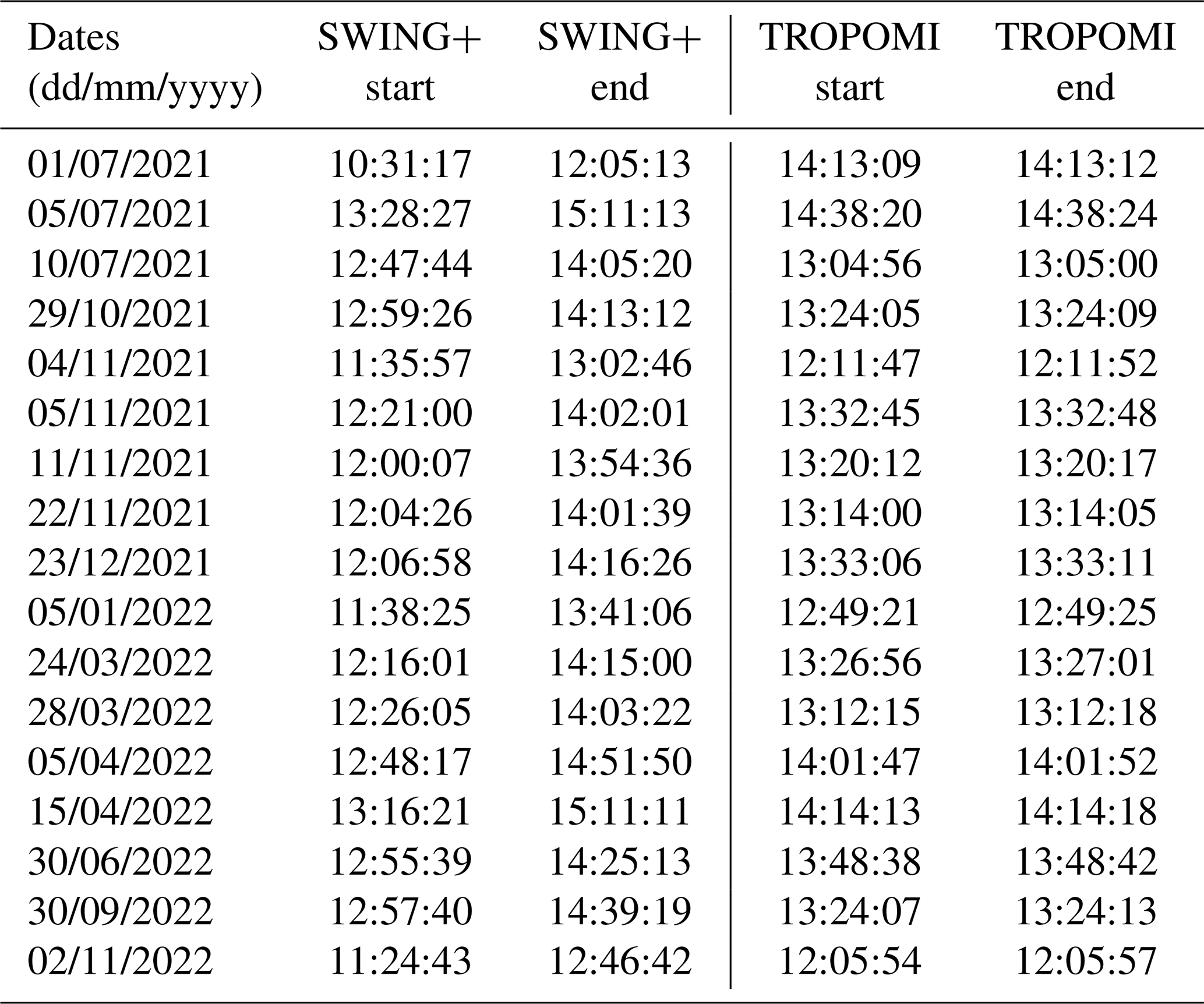
For each of the 17 SWING+ flights, listed in Table 1, we ran a WRF-Chem simulation spanning 54 h, starting at 18:00 UTC two days before the flight day and ending at 00:00 UTC the day after. This setup allows for comparisons with in situ measurements over a two-day period (including the day preceding the flight and the flight day itself), with a spin-up time of 3 or 4 h (18:00 UTC is 20:00 or 21:00 LT in Bucharest, depending on daylight saving time). For comparisons with airborne and satellite measurements, the spin-up time exceeds 37 h.

Table 1 Acquisition start and end times (local time) of the SWING+ and TROPOMI instruments for each flight date over Bucharest.

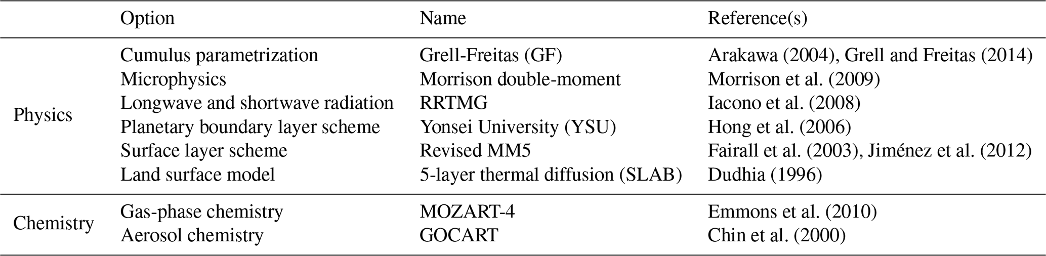
The physics and chemistry schemes and options selected for our simulations are summarized in Table 2. In addition to these choices, external data were used. More specifically, static geographical data were obtained at the highest resolutions available from the WRF users' webpage (https://www2.mmm.ucar.edu/wrf/users/download/get_sources_wps_geog.html, last access: 23 March 2026). Furthermore, we used the 0.25° × 0.25° ERA5 reanalysis data from ECMWF (Hersbach et al., 2023a, b) to provide the boundary and initial conditions for the physical parameters listed in Sect.  S1 in the Supplement. These two datasets were regridded to match our nested domains using the WPS. Boundary and initial conditions for the chemical species are obtained from the 0.95° × 1.25° WACCM6 dataset (Gettelman et al., 2019) and regridded using the mozbc preprocessor, available at the WRF-Chem Tools for the Community webpage (https://www2.acom.ucar.edu/wrf-chem/wrf-chem-tools-community, last access: 23 March 2026).

Arakawa (2004)Grell and Freitas (2014)Morrison et al. (2009)Iacono et al. (2008)Hong et al. (2006)Fairall et al. (2003)Jiménez et al. (2012)Dudhia (1996)Emmons et al. (2010)Chin et al. (2000)

Table 2 Summary of the selected physics and chemistry schemes and options used in the WRF-Chem simulations.

2.1.2 Emissions

We use the CAMS-REG inventory version 7.0 for anthropogenic emissions across the entire domain, with a spatial resolution of 0.05° × 0.1° (Kuenen et al., 2022). This inventory provides emission maps for several chemical species (CH₄, CO, NH₃, NO_x, SO_x, particulate matter, and volatile organic compounds) for each Gridded Nomenclature For Reporting (GNFR) sector, covering the years 2021 and 2022. The list of GNFR sectors, the sectoral distribution of NO_x emissions in 2021 and 2022, and the mapping from the CAMS-REG v7.0 inventory to MOZART-4 chemical species are presented in Sect. S2. The spatial distribution of NO_x emission rates, summed across all GNFR sectors and averaged over the years 2021 and 2022, is shown in Fig. 2a. Here and thereafter, we approximate the Bucharest area using the bounding box shown in Fig. 2, defined by 44.34–44.53° N and 25.96–26.24° E. Within this area, the yearly anthropogenic NO_x emissions are estimated at 32.6 mol km⁻² h⁻¹ in 2021 and 33.6 mol km⁻² h⁻¹ in 2022. These correspond to 4.03 and 4.16 kT yr⁻¹ of NO emissions, respectively. The inventory also includes additional temporal factors (hourly, daily, and monthly) and vertical profiles specific to each sector. For emissions from the GNFR sector L, which pertains to agriculture unrelated to livestock, the monthly factors vary by species. Figure 3 shows the seasonal variation of NO_x emissions over Bucharest during the simulation period. The strongest seasonal variability is associated with stationary combustion sources not related to power generation or industry, such as household energy consumption. The temporal factors are estimated based on energy consumption statistics and traffic count data (Denier van der Gon et al., 2011).

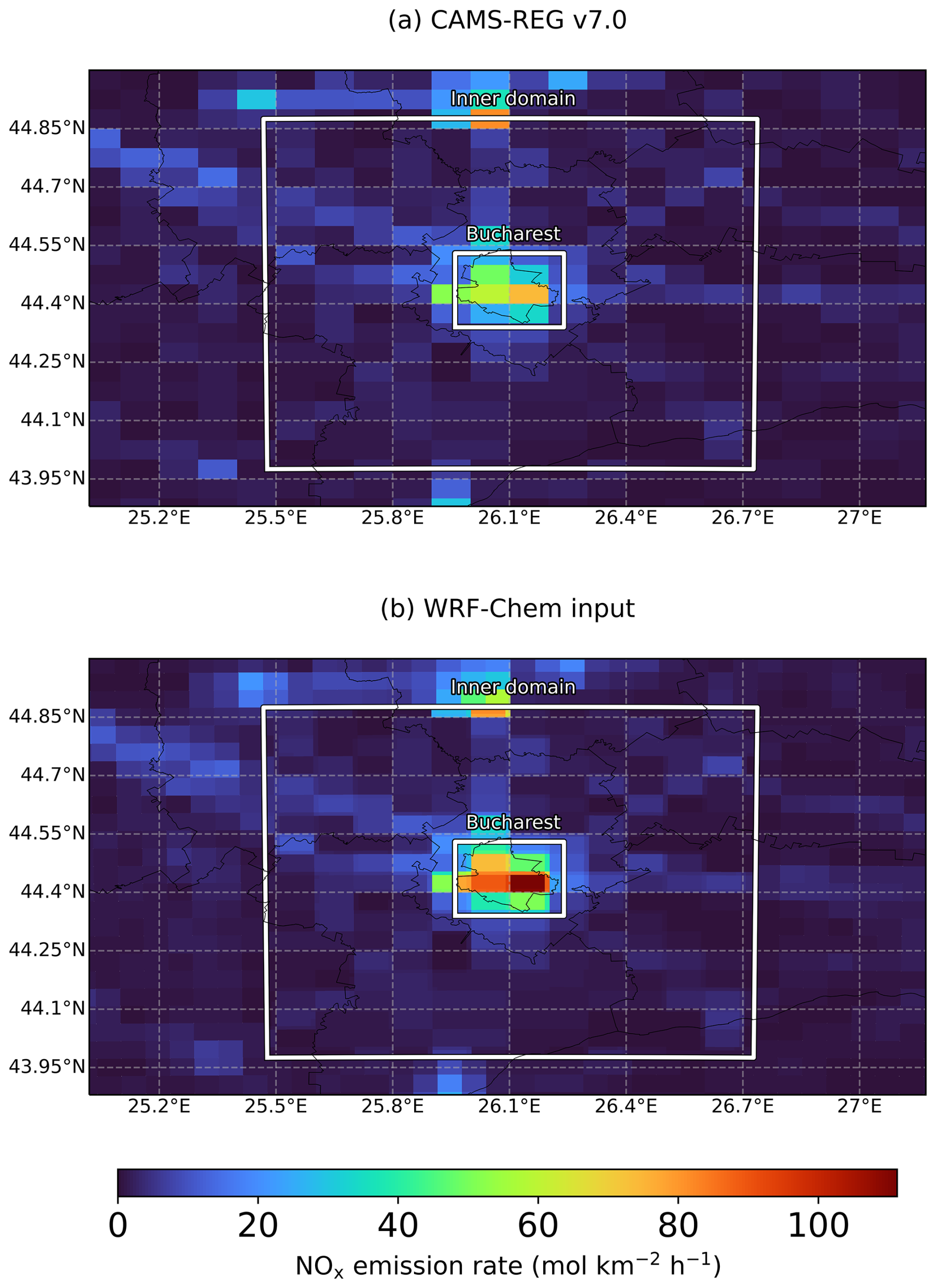
Figure 2 Distribution of NO_x emission rates over the WRF-Chem inner domain, summed across all GNFR sectors and averaged for 2021 and 2022. (a) From the CAMS-REG v7.0 inventory at its native resolution. (b) From the CAMS-REG v7.0 inventory, with the emission factor increased by a factor of 1.5 over the Bucharest box, mapped to the WRF-Chem resolution.

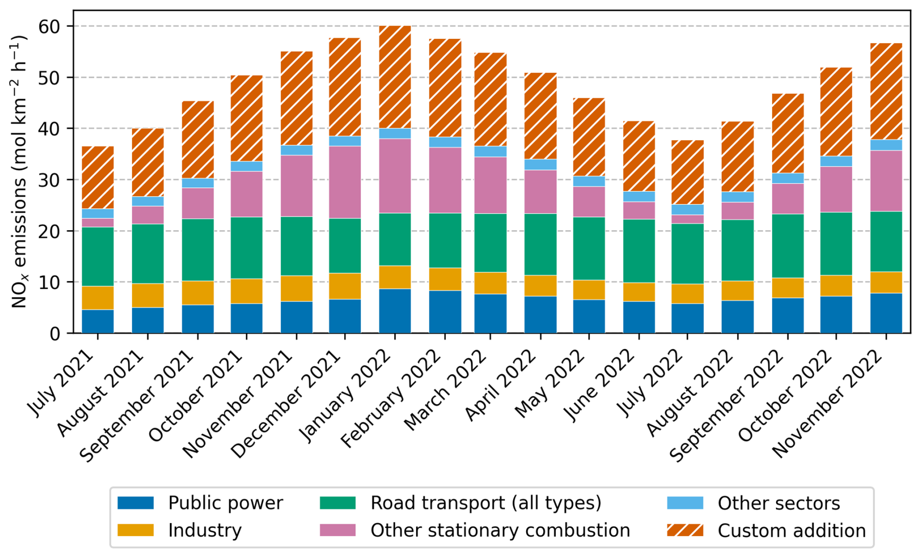
Figure 3 Seasonal distribution of anthropogenic NO_x emissions from CAMS-REG v7.0 over the Bucharest box by sector for the simulation period in 2021–2022, including the custom addition (+50 %, hatched) resulting from the upscaling of total CAMS-REG emissions.

A preliminary evaluation using in situ surface concentrations and airborne column measurements indicated that WRF-Chem NO₂ levels are generally too low over Bucharest when using CAMS-REG emissions. Therefore, we applied a custom adjustment to the CAMS-REG inventory by multiplying the NO_x emissions by a factor of 1.5 within the previously defined Bucharest box. The justification for this crude adjustment will be made clear from the model comparisons with in situ and airborne measurements (Sect. 3.1.2 and 3.2). It brings a 50 % addition (Fig. 3), raising the yearly fluxes to 48.9 mol km⁻² h⁻¹ in 2021 and 50.4 mol km⁻² h⁻¹ in 2022 over Bucharest. We handled the mapping of emissions to match WRF grid cells with a redistribution of the emission mass according to the surface fraction of each WRF grid cell within the corresponding CAMS-REG pixels, preserving the total emitted mass. The resulting map of NO_x emission rates, incorporating the adjustment for Bucharest, as provided to WRF-Chem is presented in Fig. 2b.

Biogenic emissions are computed online by WRF-Chem using the Model of Emissions of Gases and Aerosols from Nature (MEGAN) version 2.04 (Guenther et al., 2006). WRF-Chem input files for the biogenic emissions were generated using the bioemiss preprocessor, available on the WRF-Chem Tools for the Community webpage (https://www2.acom.ucar.edu/wrf-chem/wrf-chem-tools-community, last access: 23 March 2026).

Lightning-NO_x emissions are computed online based on the parametrization of Price and Rind (1992), which distributes flashes based on convective cloud top height.

2.2 Measurements

2.2.1 In situ meteorological measurements

The Măgurele center for Atmosphere and Radiation Studies (MARS), located within the WRF inner domain (yellow pin in Fig. 1b), provides measurements of air pressure, temperature, relative humidity, and solar radiation at 2 m every minute (Carstea et al., 2025). More specifically, the first three aforementioned variables are available only for the first 15 of the 17 SWING+ dates, while radiation is measured for all of them. When available, these data enable the model evaluation over two-day time series for each SWING+ flight, starting at 00:00 LT on the day preceding the flight and ending at 00:00 LT on the day after.

The national meteorological administration, Administraţia Naţională de Meteorologie (ANM), also called MeteoRomania, provides hourly measurements of air pressure, temperature, relative humidity, solar radiation at 2 m, and wind speed at 10 m (https://www.meteoromania.ro/, last access: 15 April 2026, data acquired upon request on 13 March 2024). The network operates 6 stations located within our WRF inner domain (blue pins in Fig. 1b), named after their respective localities: Afumați, Băneasa, Filaret, Oltenița, Titu, and Urziceni. For each meteorological variable, we obtained 21 or 22 measurements per flight day and at each station, with the exception of solar radiation, which was not measured at Titu and was only available for the last 8 SWING+ flight days elsewhere.

2.2.2 In situ surface chemical measurements

Surface concentrations of air pollutants are measured hourly by the national air quality monitoring network in Romania, Rețeaua Națională de Monitorizare a Calității Aerului, or RNMCA for short (https://calitateaer.ro/, last access: 23 March 2026). The network manages 30 monitoring stations in the Bucharest metropolitan area, most of which focus on particulate matter measurements. Of these, 11 stations also monitor key chemical species relevant to our study, including NO, NO₂, and for some of them also O₃. The stations are displayed in Fig. 1b. RNMCA provides information about potential pollution sources in the surroundings of each station, allowing the classification into five categories: urban, urban with traffic influence, urban in an industrial area, suburban, and rural, cf. Table 3. For the model evaluation, we consider two-day series of measurements for each SWING+ overpass. The first data point is recorded at 01:00 LT on the day preceding the flight day, and the last one 47 h later. This results in 48 data points per flight for each chemical species and each RNMCA station, provided that all measurements are available.

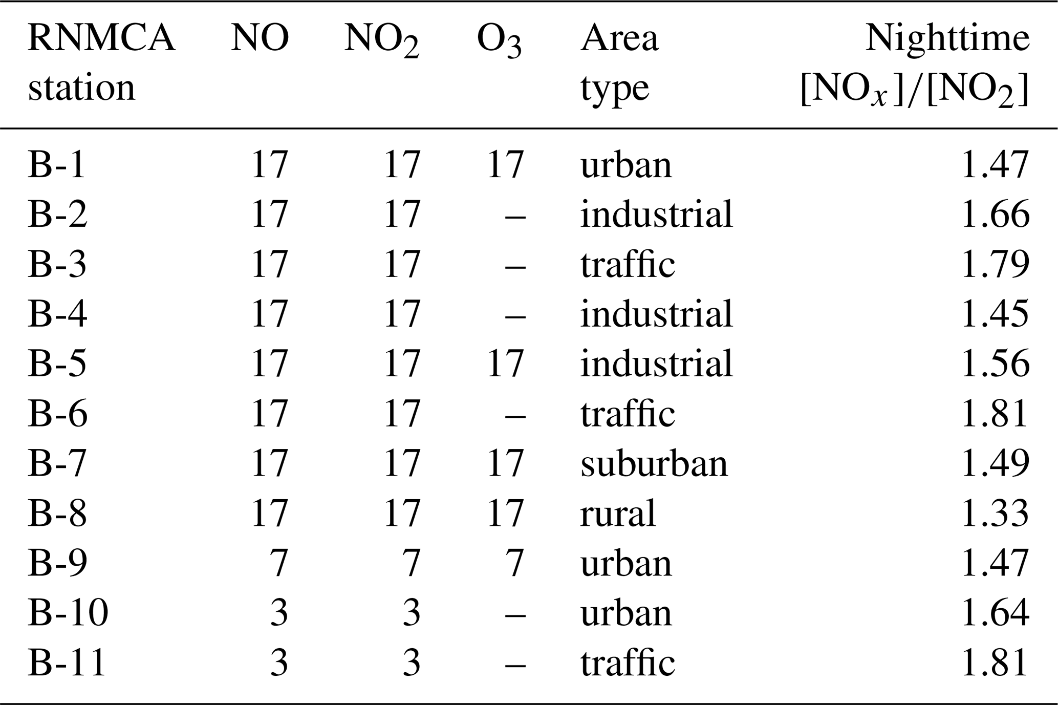
Table 3 List of RNMCA stations in the Bucharest metropolitan area that provide surface concentrations of NO, NO₂, and O₃. For each species, the number of SWING+ flight overpasses for which the RNMCA station provides in situ measurements is indicated, with 17 being the maximum. The NO${}_x/{\mathrm{NO}}_{\mathrm{2}}$ ratio is calculated as the average of the hourly ratios evaluated at night across all two-day measurement series and serves as a criterion for assessing the model representativity at each station.

The chemiluminescence measurement of NO₂, which uses a molybdenum converter, is known to be affected by interference from compounds in the NO_y reservoir (Lamsal et al., 2008). The modeled mixing ratio of NO₂ should therefore account for contributions from PAN, HNO₃, and the sum of alkyl nitrates. The latter includes the (reactive) organic nitrate species, ONIT and ONITR, which are present in the MOZART-4 mechanism. We compute the corrected modeled volume mixing ratio of NO₂, referred to as ${\mathrm{NO}}_{\mathrm{2}}^{*}$, from the WRF-Chem model output following Lamsal et al. (2008):

$$\begin{array}{}\text{(1)}& \begin{array}{rl}\left[{\mathrm{NO}}_{\mathrm{2}}^{*}\right]& =\left[{\mathrm{NO}}_{\mathrm{2}}\right]+\mathrm{0.95}\left[\mathrm{PAN}\right]+\mathrm{0.35}\left[{\mathrm{HNO}}_{\mathrm{3}}\right]+\left[\mathrm{ONIT}\right]\\ & +\left[\mathrm{ONITR}\right].\end{array}\end{array}$$

Hereafter, the measured surface NO₂ will be referred to as ${\mathrm{NO}}_{\mathrm{2}}^{*}$ as well.

Some RNMCA sites are closer to NO_x pollution sources than others and are more likely to show higher NO_x concentrations than the model prediction due to enhanced representation errors. Poraicu et al. (2025) suggested that the measured nighttime NO${}_x/{\mathrm{NO}}_{\mathrm{2}}$ ratio can be used to determine whether a station is well represented by the model. Indeed, away from emission sources, NO_x species are expected to reach the pseudo-steady state (PSS) of their photochemical cycle, which constrains the NO${}_x/{\mathrm{NO}}_{\mathrm{2}}$ ratio:

$$\begin{array}{}\text{(2)}& {\left({\displaystyle \frac{\left[{\mathrm{NO}}_x\right]}{\left[{\mathrm{NO}}_{\mathrm{2}}\right]}}\right)}_{\text{PSS}}=\mathrm{1}+{\displaystyle \frac{J}{k\left[{\mathrm{O}}_{\mathrm{3}}\right]+\mathrm{\dots }}},\end{array}$$

where J is the photolysis rate of NO₂, $k=\mathrm{1.95}\times {\mathrm{10}}^{-\mathrm{14}}$ molec.⁻¹ cm³ s⁻¹ (at 298 K) is the rate constant for the titration of O₃ with NO (Burkholder et al., 2019), and the dots represent contributions from peroxy radicals. At night, J becomes negligible, causing the ratio to decrease and approach 1. However, photochemical equilibrium is far from being achieved near NO_x pollution sources, which primarily emit NO and lead to observed ratios significantly higher than 1. Thus, we select RNMCA stations with relatively low measured NO${}_x/{\mathrm{NO}}_{\mathrm{2}}$ ratios (using ${\mathrm{NO}}_{\mathrm{2}}^{*}$ measured values to represent NO₂ in both the numerator and denominator) during nighttime, in order to exclude the least representative stations. As shown in Table 3, stations influenced by traffic exhibit the largest deviations from the PSS prediction, with nighttime ratios greater or equal to 1.79. As expected, the lowest ratio (1.33) is found for the only rural station. For the model evaluation in Sect. 3.1.2, we will focus on the eight stations not directly exposed to traffic, characterized by a nighttime NO${}_x/{\mathrm{NO}}_{\mathrm{2}}$ ratio below 1.7 (B-1, B-2, B-4, B-5, B-7, B-8, B-9, and B-10). The enhancement of ${\mathrm{NO}}_{\mathrm{2}}^{*}$ concentrations at traffic stations is not specific to our selected dates but was also observed in yearly averages from 2020 to 2022, as reported by Ilie et al. (2023). Note that this distinction does not affect the analysis of O₃ concentrations, as traffic stations do not measure it. Ozone is only monitored at five distinct stations (Table 3).

2.2.3 Airborne SWING+ NO₂ column measurements

SWING (Small Whiskbroom Imager for atmospheric compositioN monitorinG) instruments are compact whiskbroom imagers developed at BIRA-IASB for air quality mapping. They use ultraviolet and visible-light spectrometers, covering a spectral range of 280–550 nm with a resolution of 0.7 nm Full Width Half Maximum (FWHM), to retrieve NO₂ column abundances using the Differential Optical Absorption Spectroscopy (DOAS) technique (Platt and Stutz, 2008). Initially designed for operations onboard an unmanned aerial vehicle (UAV) (Merlaud et al., 2018), SWING instruments have since been deployed on crewed aircraft for validation flights alongside ground-based DOAS instruments and larger airborne imagers over Berlin, Germany (Tack et al., 2019), and over Bucharest and an isolated power plant in Romania (Merlaud et al., 2020). Observations with SWING instruments demonstrated their capability to resolve urban and industrial plumes, ranging from 10¹⁵ to 20×10¹⁵ molec. cm⁻² in Berlin, and up to 80×10¹⁵ molec. cm⁻² in Romania. In both intercomparison studies, Pearson correlation coefficients exceeded 0.9, and linear regression slopes were close to unity with intercepts below 10¹⁵ molec. cm⁻². Over Bucharest, SWING biases were estimated within 28 % (accounting for temporal lags with the satellite overpass; Merlaud et al., 2020), indicating its suitability for TROPOMI tropospheric NO₂ validation, as this falls below the satellite mission requirement of 50 % (Veefkind et al., 2012).

The SWING observations over Bucharest exploited in this study originate from two ESA-funded projects: RAMOS (Nemuc et al., 2023) and QA4EO (Nemuc et al., 2024). Within RAMOS, a custom version of the instrument, named SWING+, was developed at BIRA-IASB and permanently installed on the Britten-Norman 2 (BN-2) aircraft operated by INCAS (National Institute for Aerospace Research). Compared to the original UAV version, SWING+ is enclosed in an aluminum casing, with the scanner deported by 20 cm to exit the aircraft fuselage. The instrument is still relatively compact ($\mathrm{45}\times \mathrm{19}\times \mathrm{15}$ cm³, 3.8 kg).

In contrast to typical field campaigns that are deployed over a few weeks during summer, the flight strategy in RAMOS and QA4EO consisted in flying on a regulatory basis across the year, limited to clear-sky conditions. The BN-2 flew over the city from an altitude of 3 km, and the SWING+ swath was set to 48°, incremented in steps of 6°, with an integration time of 0.5 s. This configuration resulted in a ground resolution of 0.35×0.35 km². Table 1 lists the 17 flights used in this study, operated between July 2021 and November 2022. All dates are weekdays, except for 10 July 2021, which was a Saturday. Flight times were chosen to coincide with TROPOMI overpasses, except for the first date which was the test flight.

SWING+ measurements are filtered based on the DOAS optical depth fit; measurements with root mean square (RMS) residuals greater than $\mathrm{5}\times {\mathrm{10}}^{-\mathrm{3}}$ are rejected. Each vertical column density (VCD, or Ω_S when specifically referring to SWING+) of NO₂ is then obtained by dividing the slant column density (SCD) by an air mass factor (AMF) specific to each measurement. The slant column itself is the sum of a reference slant column density (SCD_ref), estimated only once per flight, and the differential slant column density (DSCD):

$$\begin{array}{}\text{(3)}& \text{VCD}={\displaystyle \frac{\text{SCD}}{\text{AMF}}}={\displaystyle \frac{{\text{SCD}}_{\text{ref}}+\text{DSCD}}{\text{AMF}}}.\end{array}$$

AMFs are calculated with the Vector Linearized Discrete Ordinate Radiative Transfer model (VLIDORT; Spurr, 2008) version 2.7. For radiometrically calibrated instruments such as APEX (Tack et al., 2019), surface reflectance can be retrieved through atmospheric correction of at-sensor radiance. However, for most airborne instruments (e.g., SWING+, AirMAP, Spectrolite; Tack et al., 2019), such calibration is not available. For SWING+, the albedo is therefore derived from MODIS surface properties, providing black-sky albedo at 470 nm (MCD43A3 v006; Schaaf and Wang, 2015) interpolated to each airborne pixel. The a priori profile is a well-mixed NO₂ box profile constrained by the ERA5 planetary boundary layer (PBL) height (Hersbach et al., 2023b), under the assumption that the large majority of NO₂ resides within the PBL. Clouds are not accounted for in the algorithm, as flights were planned and mostly conducted under cloud-free conditions, except for 4 out of the 17 dates¹ (5 July 2021, 5 November 2021, 23 December 2021, and 15 April 2022). Errors in AMF calculations are then mainly driven by surface albedo, NO₂ vertical profiles, and aerosol properties. For the SWING+ campaign, this uncertainty is estimated at 15.2 %, based on a sensitivity analysis by Tack et al. (2017).

SCD_ref represents a residual correction that accounts for the NO₂ amount present in the instrument reference spectrum. The reference spectrum is updated for each flight and calculated as the average of 30 spectra recorded over a clean area. This correction, associated with the average spectrum, was then estimated using interpolated SCD NO₂ data from TROPOMI (Veefkind et al., 2012). SCD_ref values range from 0.5 to 2.1×10¹⁵ molec. cm⁻², with an uncertainty estimated at 100%, yielding an error of 0.2–1.0 ×10¹⁵ molec. cm⁻² after division by the AMF. Averaged per flight day, the DSCD uncertainty ranges from 1.4–2.5 ×10¹⁵ molec. cm⁻², reducing to 0.5–1.6 ×10¹⁵ molec. cm⁻² once divided by the AMF. The combined contributions of the AMF, SCD_ref, and DSCD yield a total VCD uncertainty of 0.9–1.9 ×10¹⁵ molec. cm⁻². Lower uncertainties correspond to lower VCDs observed in spring and summer, while higher uncertainties are associated with elevated columns in fall and winter.

For the evaluation of the WRF-Chem model, SWING+ vertical column densities and averaging kernels are regridded to the model resolution. Measurements falling within the same WRF grid cell and separated in time by less than the model output interval (5 min) are averaged to produce a single regridded SWING+ column. After regridding, the daily average VCD error due to DSCD uncertainty, which is primarily of random origin, decreases to 0.3–0.7 ×10¹⁵ molec. cm⁻². Systematic errors remain unaffected by the regridding. The same process is applied to the averaging kernels, denoted as A_S, which are then used to evaluate the modeled columns, accounting for the instrument vertical sensitivity. More precisely, WRF-Chem NO₂ tropospheric columns Ω_W,S are derived from the modeled NO₂ density field n_W and the regridded kernels by integrating over the troposphere (Trop):

$$\begin{array}{}\text{(4)}& {\mathrm{\Omega }}_{\text{W},\text{S}}=\underset{\text{Trop}}{\int }{A}_{\text{S}}\left(z\right)n_{\text{W}}\left(z\right)\mathrm{d}z.\end{array}$$

The regridding of SWING+ measurements for the purpose of TROPOMI validation is detailed in the next section.

2.2.4 Satellite-borne TROPOMI NO₂ column measurements

The TROPOspheric Monitoring Instrument (TROPOMI) was launched aboard the Sentinel-5 Precursor (S5P) satellite of the European Space Agency in October 2017 to monitor atmospheric composition and air quality (Veefkind et al., 2012). S5P is a near-polar and sun-synchronous satellite with a near-daily overpass. TROPOMI is a nadir-viewing pushbroom imaging spectrometer that covers spectral bands in the ultraviolet, visible, near-infrared, and shortwave infrared regions, enabling the retrieval of key atmospheric trace gases, including NO₂. Its spatial resolution was initially 7 × 3.5 km², and improved to 5.5 × 3.5 km² after August 2019. Its overpass times over Bucharest are listed in Table 1.

The TROPOMI tropospheric NO₂ vertical column density Ω_T is generated through a multi-step retrieval process. First, DOAS is applied to the Level-1b radiance and irradiance spectra to retrieve total slant column densities in the 405–465 nm range, using techniques developed for OMI (van Geffen et al., 2020). Second, the separation of stratospheric and tropospheric contributions is performed using data assimilation in the TM5-MP chemistry transport model (Williams et al., 2017). In the final step, the tropospheric slant column is converted to a vertical column using air mass factors (AMFs), which are computed with the Doubling-Adding KNMI radiative transfer model (de Haan et al., 1987; Stammes, 2001) based on TM5-MP NO₂ vertical profiles. Further details are provided in the TROPOMI NO₂ Algorithm Theoretical Basis Document (van Geffen et al., 2024).

In this study, we evaluate TROPOMI NO₂ retrievals from version 2.4.0, using reprocessed data (RPRO) up to 17 July 2022 and the offline product (OFFL) thereafter (Eskes et al., 2024). This version incorporates an updated surface albedo climatology based on TROPOMI observations. Only measurements with a quality assurance value greater than 0.75 are retained, in accordance with the recommendation. Additionally, only those TROPOMI measurements for which at least 50 % of the pixel area is covered by SWING+ observations are considered in the analysis. The average precision of these TROPOMI measurements is 1.3×10¹⁵ molec. cm⁻².

SWING+ measurements are used here to validate TROPOMI, with WRF-Chem serving as an intercomparison platform that accounts for the acquisition times and vertical sensitivities of both instruments. The validation is carried out in two steps:

1. We assess the bias of WRF-Chem relative to SWING+ and determine the appropriate correction to WRF-Chem columns for each flight. This is realized at the TROPOMI spatial resolution by averaging both SWING+ and the corresponding WRF-Chem columns Ω_W,S over TROPOMI pixels. At this resolution, the random uncertainty on the SWING+ column stemming from the DSCD, presented in the previous section, falls below 10¹⁴ molec. cm⁻². Although model errors arise from both random and systematic sources, they are expected to be correlated from pixel to pixel within the short time window (typically less than 2 h; see Table 1) and small spatial domain (Bucharest surroundings). These correlated errors are therefore treated as systematic and identified with the model bias, which is allowed to vary from one flight day to the next. Any remaining random component of the model error is further reduced through regridding to the TROPOMI resolution.

2. We evaluate another set of WRF-Chem columns, denoted as Ω_W,T, using TROPOMI averaging kernels A_T and the modeled NO₂ density profile n_W averaged over TROPOMI pixels:

   $$\begin{array}{}\text{(5)}& {\mathrm{\Omega }}_{\text{W},\text{T}}=\underset{\text{Trop}}{\int }{A}_{\text{T}}\left(z\right)n_{\text{W}}\left(z\right)\mathrm{d}z,\end{array}$$

   and correct these columns based on the biases evaluated in the first step. The bias-corrected version of Ω_W,T columns, denoted by ${\mathrm{\Omega }}_{\text{W},\text{T}}^{\text{bc}}$, then serve as a reference to evaluate the bias of TROPOMI, combining data from different flight days, either all together or by season.

In both steps, we assume that the biases of the model and the satellite can be captured through linear regression against reference values. Both parametric and robust linear regression methods (Theil–Sen estimator; Theil, 1950; Sen, 1968) are tested, with the latter suppressing the impact of outliers. Importantly, the resulting linear corrections not only adjust mean column magnitudes but also modify spatial gradients to first order, as the bias is estimated as a concentration-dependent quantity. To ensure the quality of the results, a selection of flight days will be made based on the evaluation of the model against SWING+ data. Note that this method generalizes the approach of Poraicu et al. (2023) by extending it to simultaneously address multiple flight days. In their study, WRF-Chem biases relative to the airborne instrument APEX and to TROPOMI were subtracted to infer the bias of TROPOMI with respect to APEX, one flight date at a time.

3 Results

3.1 Model evaluation using in situ measurements

3.1.1 Meteorological observations

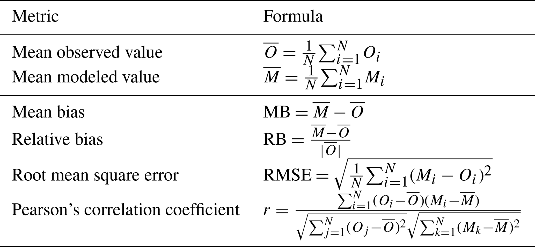
In this section, we present the results of the model evaluation for the surface values of physical parameters measured at the MARS and ANM stations. The analysis combines the observed and modeled physical parameters from all 17 flight dates, over the corresponding two-day periods at MARS and the flight days for the ANM stations (see Fig. 4). Details about the synoptic parameters specific to individual SWING+ flight days that could be critical for the evaluation of the NO₂ column, such as the modeled wind direction over the city during the flight time, will be discussed in Sect. 3.2. Throughout this study, we use the statistical metrics defined in Table 4.

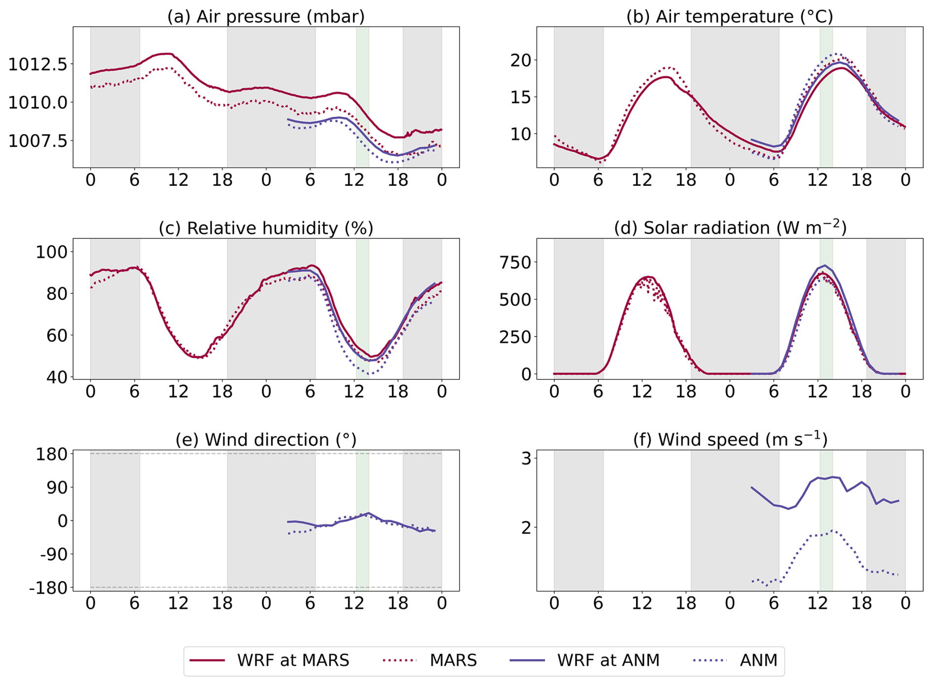
Figure 4 Surface meteorological measurements from MARS and ANM and comparison with WRF-Chem. The horizontal axes represent local time in hours. Each plot focuses on a specific meteorological parameter and includes all 17 one or two-day time series from the various stations, when available, averaged into a single time series. Some points were excluded from the plots when the number of available station-date pairs fell below 95 % of the maximum, as this was considered unrepresentative visually, though the data is still included in the main text analysis. Gray and green windows indicate the averaged nighttime and SWING+ flight hours from the measurement dates, respectively.

Table 4 Statistical metrics used to evaluate the model. The formulas are written for N observed values O_i and the corresponding modeled data M_i, with $i=\mathrm{1},\mathrm{\dots },N$.

The model mean bias (MB) for air pressure is 1.0 mbar at MARS, 0.4 mbar at the ANM stations, and overall negligible in terms of relative biases. The corresponding root mean square error (RMSE) are 1.2 and 0.9 mbar, respectively. Both measurement datasets show a perfect correlation coefficient of 1.00. The air temperature measurements indicate model biases of −0.4 °C at MARS and 0.1 °C at the ANM stations. The daytime underestimation and nighttime overestimation of temperature were reported in a previous study using the WRF model over Bucharest (Iriza et al., 2017). The model RMSE reach 2.3 and 2.4 °C, respectively. The correlation remains excellent overall, with Pearson's coefficients of 0.98 and 0.97. The MB of the model for relative humidity reach 2.1 % at MARS and 5.4 % at the ANM stations. RMSEs are an order of magnitude higher, 11.5 % and 14.2 %, respectively. High correlations, with values of 0.86 and 0.85, are calculated at the corresponding sites. Solar radiation is well reproduced by the model according to MARS measurements: the MB of 9.2 W m⁻² is negligible, the RMSE is 66.7 W m⁻², and the correlation is close to 1 (0.97). Generally, fewer fluctuations are observed on the second day, see Fig. 4d, as it was selected as the flight day due to favorable weather conditions. The good model performance is further confirmed with the ANM measurements, despite an increase in bias and error: the MB is 36.5 W m⁻², the RMSE is 69.8 W m⁻², and the correlation coefficient is equal to 0.99. The ANM measurements indicate an overestimation of the modeled wind speed by 1.0 m s⁻¹, in line with former WRF evaluations over urban areas (Kim et al., 2013; Feng et al., 2016; Poraicu et al., 2023). The wind direction is biased by 15.7°. Evaluating both components of the modeled horizontal wind field, U and V, the RMSE is 1.5 m s⁻¹ and we find a Pearson's correlation coefficient of 0.64.

3.1.2 Surface chemical concentrations

We compare surface concentration measurements from the RNMCA network with WRF-Chem for NO, ${\mathrm{NO}}_{\mathrm{2}}^{*}$, and O₃ at the model lowest vertical level. Figure 5 displays the model performance for the different types of stations. Each plot includes measurements from the 17 two-day time series, averaged into a single time series. Therefore, the discussion of seasonality is deferred to a later part of this section.

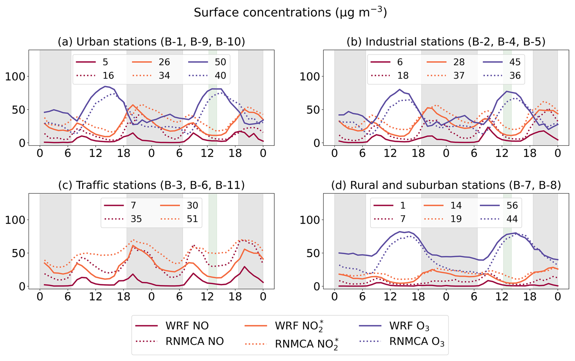
Figure 5 Comparison of surface NO, ${\mathrm{NO}}_{\mathrm{2}}^{*}$, and O₃ measurements from the RNMCA network with WRF-Chem model outputs. Units of the vertical and horizontal axes are µg m⁻³ and hours (local time). Each plot focuses on a specific set of RNMCA stations based on location and includes all 17 two-day time series, when available, averaged into a single time series. For each series, we indicate the mean value in the legend. Gray and green windows indicate the averaged nighttime and SWING+ flight hours from the measurement dates, respectively.

The model generally underestimates NO and ${\mathrm{NO}}_{\mathrm{2}}^{*}$ levels while overestimating O₃, in line with the strong titration effect of NO_x on ozone near pollution sources. The underestimation of ${\mathrm{NO}}_{\mathrm{2}}^{*}$ is significantly reduced when moving from traffic stations (−21 µg m⁻³) to suburban and rural stations (−5 µg m⁻³). This aligns with the discussion on station representativeness in Sect. 2.2.2 and further supports the exclusion of traffic stations when selecting representative sites. We therefore present in Table 5 the statistical metrics used to evaluate the 17 two-day time series, focusing only on non-traffic stations. Another table is presented in Sect. S3, comparing simulations with and without the 1.5 scaling factor applied to NO_x emissions. In the unscaled case, the underestimation of NO and ${\mathrm{NO}}_{\mathrm{2}}^{*}$, and the corresponding overestimation of O₃ levels, are slightly more pronounced, by a few percent.

The negative bias in daytime ${\mathrm{NO}}_{\mathrm{2}}^{*}$ levels in WRF-Chem is similar to the reported underestimation by Poraicu et al. (2023). However, WRF-Chem simulations over Europe have shown an important nighttime overestimation of ${\mathrm{NO}}_{\mathrm{2}}^{*}$ (Poraicu et al., 2023; Kuhn et al., 2024), which is not observed here. Our results also contrast with those from the Land-Use Regression model (Talianu et al., 2025), which reported daytime positive biases of 8 %–30 % during a period within 2022 and 2023, using a comparable set of measurements over Bucharest.

Several factors may explain this discrepancy. While an underestimation of emissions remains a possibility, comparisons with NO₂ column measurements in the following sections suggest that the factor of 1.5 applied to the CAMS-REG inventory is well-justified. However, other factors could also contribute to the model underestimation:

• Poor representativeness of measurements: Even at non-traffic stations, nighttime NO${}_x/{\mathrm{NO}}_{\mathrm{2}}$ ratios remain significantly higher than 1 (see Table 3).

• Limited resolution of anthropogenic emissions: The CAMS-REG inventory is too coarse to accurately capture the spatial heterogeneity of the city, leading to an underestimation of NO_x pollution levels near hotspots.

• Overestimated surface wind: As seen in Sect. 3.1.1, the model overestimates horizontal wind speed, which enhances the advection of clean air from surrounding rural areas, diluting NO_x concentrations.

• Excessive vertical mixing: Turbulence in the boundary layer could further contribute to the dilution of NO_x species. Unfortunately, the lack of ceilometer data prevents us from diagnosing potentially overestimated vertical mixing.

Table 5 Statistical metrics calculated for each species and period of the day. Values are obtained from non-traffic RNMCA stations and flight hours refer to the SWING+ acquisition times.

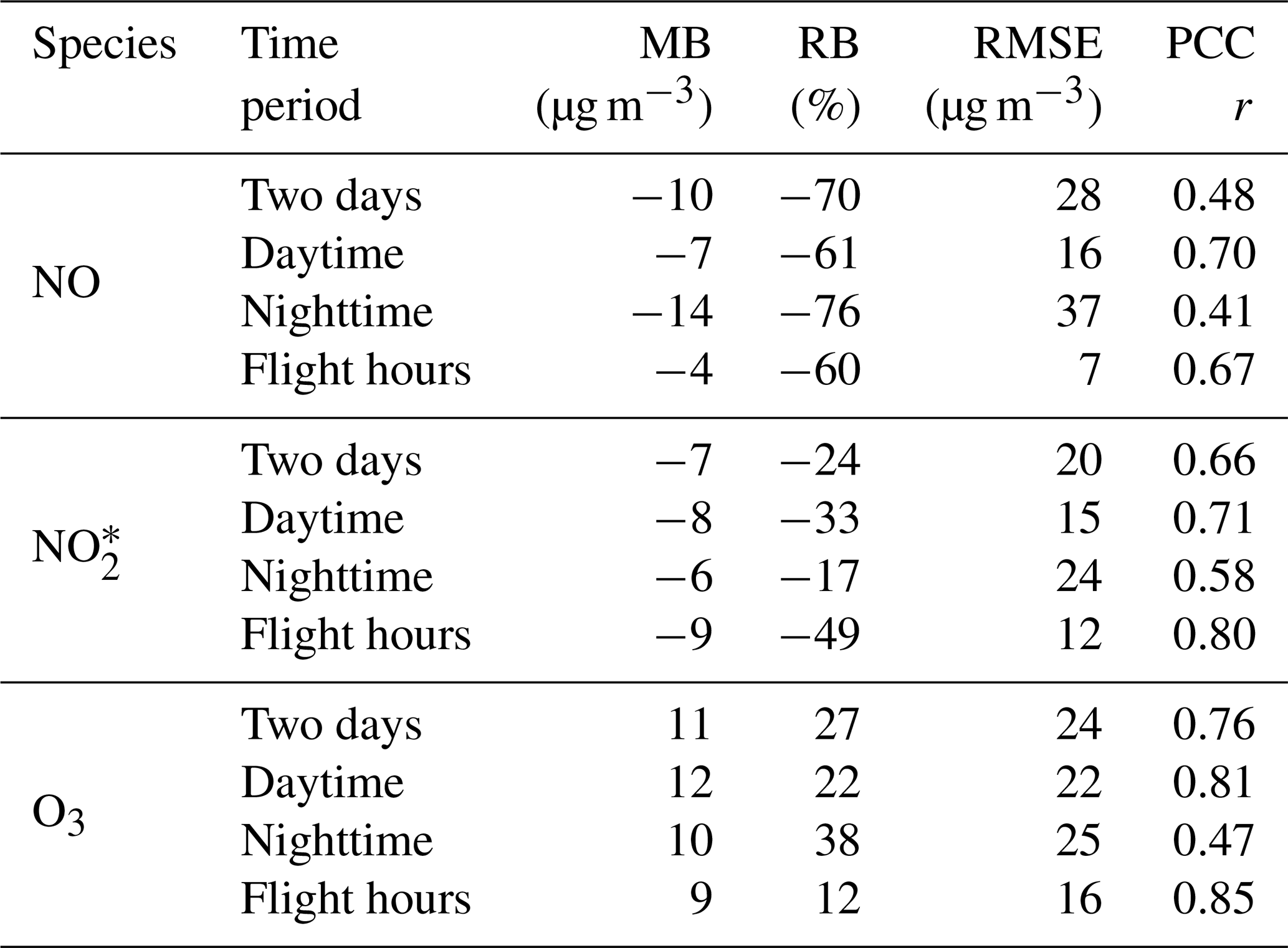
The model generally captures well the diurnal cycle of the measurements. The rush hour peak in the morning and the evening peak in NO_x are observed in both the measured and modeled concentrations. As pointed out by Poraicu et al. (2023), a rush hour peak in the late afternoon is not always identifiable, which is expected due to the counterbalancing effects of chemical sink and boundary layer development. The daytime ozone buildup and plateau are well reproduced by the model. Slight delays in these patterns may occur, but the overall correlation is satisfactory. During daytime, we report in Table 5 correlation coefficients of 0.70, 0.71, and 0.81 for NO, ${\mathrm{NO}}_{\mathrm{2}}^{*}$, and O₃, respectively. Notably, if we restrict the time window to flight hours for ${\mathrm{NO}}_{\mathrm{2}}^{*}$, in anticipation of the SWING+ measurements analysis, the correlation increases to 0.80.

The two-day simulation periods may be grouped according to the meteorological seasons. Figure 6 compares the measured values at non-traffic RNCMA stations with the corresponding modeled outputs, separated by season: summer (June–August), fall (September–November), winter (December–February), and spring (March–May).

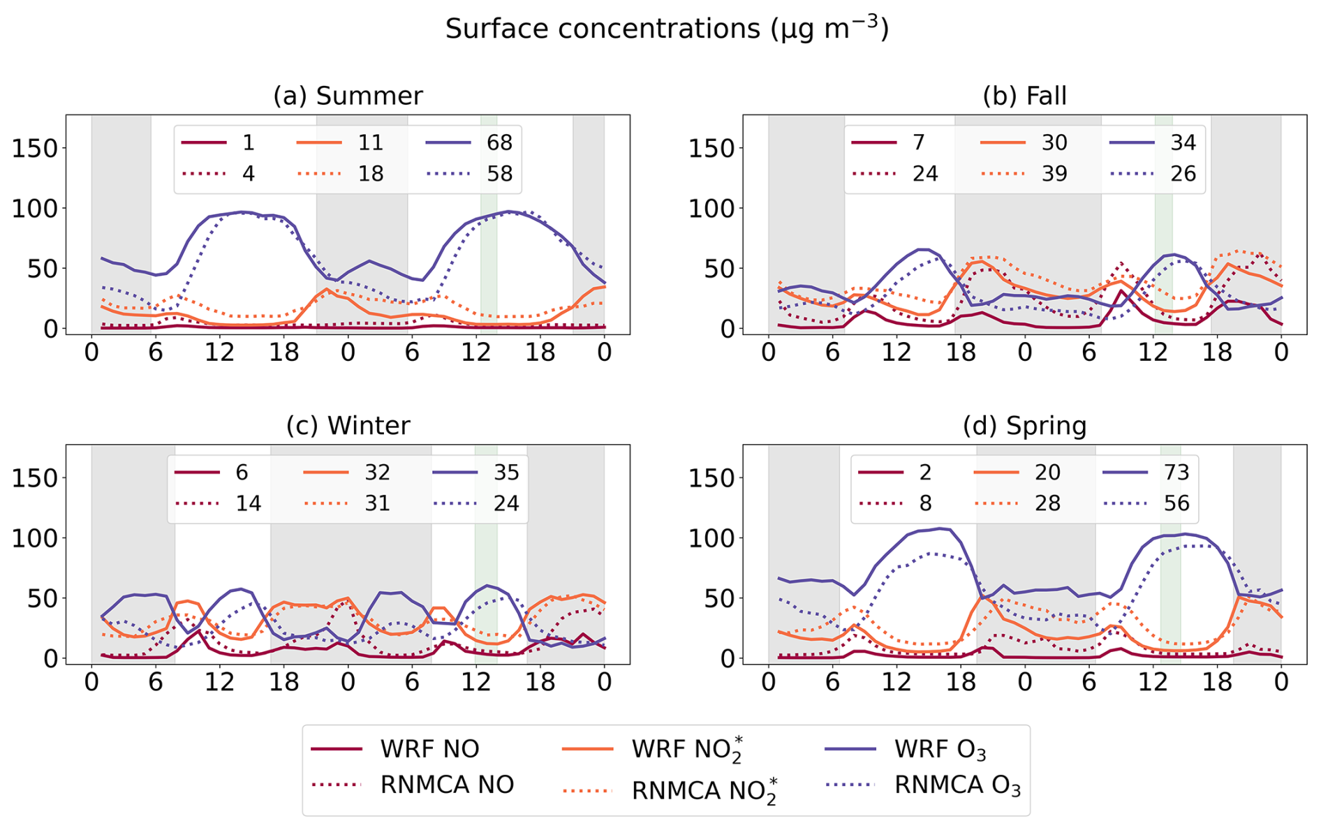
Figure 6 Comparison of surface RNMCA measurements from non-traffic stations with WRF-Chem model outputs. Units of the vertical and horizontal axes are µg m⁻³ and hours (local time). Each plot is the averaged curve of series of two-days on a specific meteorological season: summer (4 series), fall (7 series), winter (2 series), and spring (5 series). For each two-day series, we indicate the mean value of the surface concentration in the legend. Gray and green windows indicate the averaged nighttime and SWING+ flight hours from the measurement dates, respectively.

NO peaks are sharper during cold months. This is due to lower sun exposure in winter, which reduces the generation of ozone and peroxy radicals, both of which are sinks for NO, thereby increasing its lifetime as well as the time needed to reach photochemical steady state between NO and ${\mathrm{NO}}_{\mathrm{2}}^{*}$. As in the previous analysis, we find that NO levels are generally underestimated by the model across all seasons. In particular, the model does not simulate enough nighttime accumulation during the colder months. The second day of the winter runs shows the best daytime agreement, relative to other seasons. However, because the winter analysis is based on only two time series, it is difficult to draw definitive conclusions regarding which season is best reproduced by the model. Daytime correlation values remain consistent across seasons, ranging from 0.60 in winter to 0.68 in fall. Note that in summer, measurements are close to the detection limit.

Similarly to NO, surface levels of ${\mathrm{NO}}_{\mathrm{2}}^{*}$ are generally underestimated. The best agreement is found in winter, where nighttime values appear to be particularly well reproduced. The diurnal evolution during this season is also well captured, though with greater variation. The morning rush hour peak is visible in the modeled values for fall and spring but is too flat during summer. Daytime correlation coefficients range from 0.59 in summer to 0.73 in winter.

Ozone is consistently overestimated across all seasons, both during day and night. As expected, months with higher sun exposure exhibit a more significant O₃ buildup, generated from the oxidation of carbon monoxide and volatile organic compounds in presence of NO_x and ultraviolet radiation. This seasonal variability is present in both the measured and modeled values (in value ranges comparable to those observed in the WRF-Chem simulations of Maco et al., 2019). Notably, a good agreement is found at the summer daytime maxima. Daytime correlation is lower in winter, with a coefficient of 0.49, while in other seasons, it ranges from 0.75 to 0.79.

3.2 Model evaluation against airborne column measurements

For each flight, column comparisons are assessed using the statistical metrics of Table 4. The results vary significantly from one date to the next. Therefore, we will first provide a detailed analysis only for the two flight days with the highest correlation coefficient, 11 November 2021 and 30 June 2022, before presenting a summary encompassing all flight days.

3.2.1 Flight on 11 November 2021

The temporal series and maps in Fig. 7 illustrate the model capability to reproduce tropospheric NO₂ columns on our best-performing date. The observed and modeled NO₂ levels are very similar, and the synchronicity of the peaks and dips in the time series leads to an excellent correlation coeffcient of 0.94. The maps clearly show a plume emanating from the city and transporting NO₂ in the North-West direction in both cases. This is a satisfactory result considering the coarse resolution of the emission inventory.

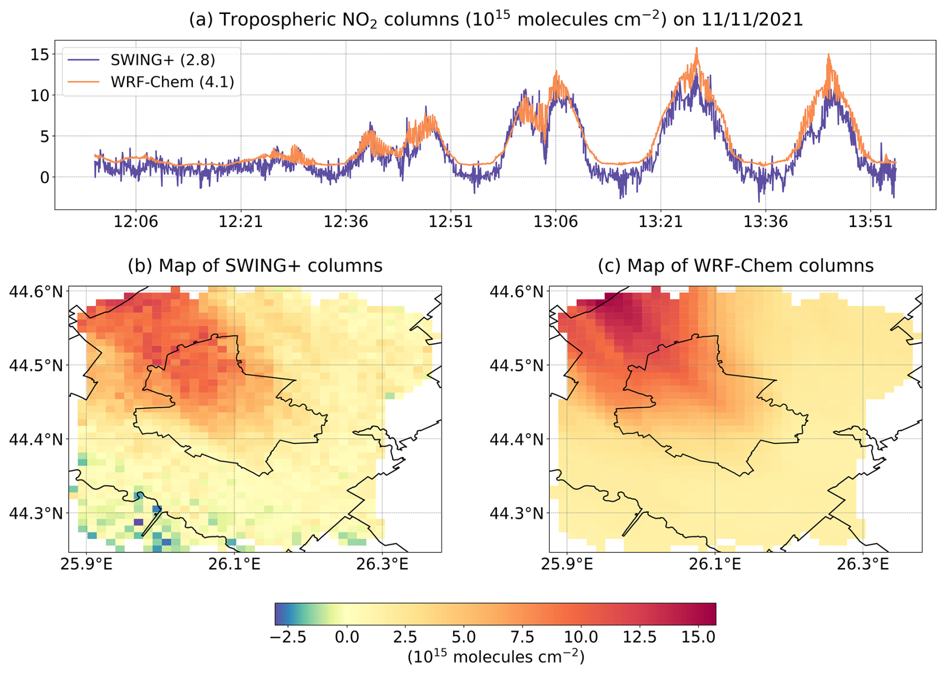
Figure 7 Tropospheric NO₂ columns on Thursday 11 November 2021, presented as a temporal series of SWING+ and WRF-Chem values plotted against local time, with mean values in parentheses in (a), and corresponding maps in (b) and (c).

The calculated RMSE is equal to 1.7×10¹⁵ molec. cm⁻², mainly due to an overestimation, both in the background values and at the plume peaks. The relative bias (RB) is relatively high (43 %), partly due to the large number of small values, including negative ones, in the SWING+ measurements. Note that negative values may result from a calibration offset combined with random errors in the background values. For this flight, only 2.3 % of the measurements are negative and within the bounds of the error bar.

3.2.2 Flight on 30 June 2022

Figure 8 presents the model evaluation on 30 June 2022. The first part of the airborne measurements shows abnormally high background values away from the plume emanating from the city (cf. dotted area in the subfigures). Those high values are not captured by the model and are likely due to a stabilization delay of the SWING+ instrument. Specifically, since the SWING+ instrument is not thermally stabilized, its spectral resolution changes as the temperature decreases during the flight ascent. These variations affect the accuracy of the NO₂ measurements. For this reason, we exclude the first measurements, up to 13:24 LT, from our analysis.

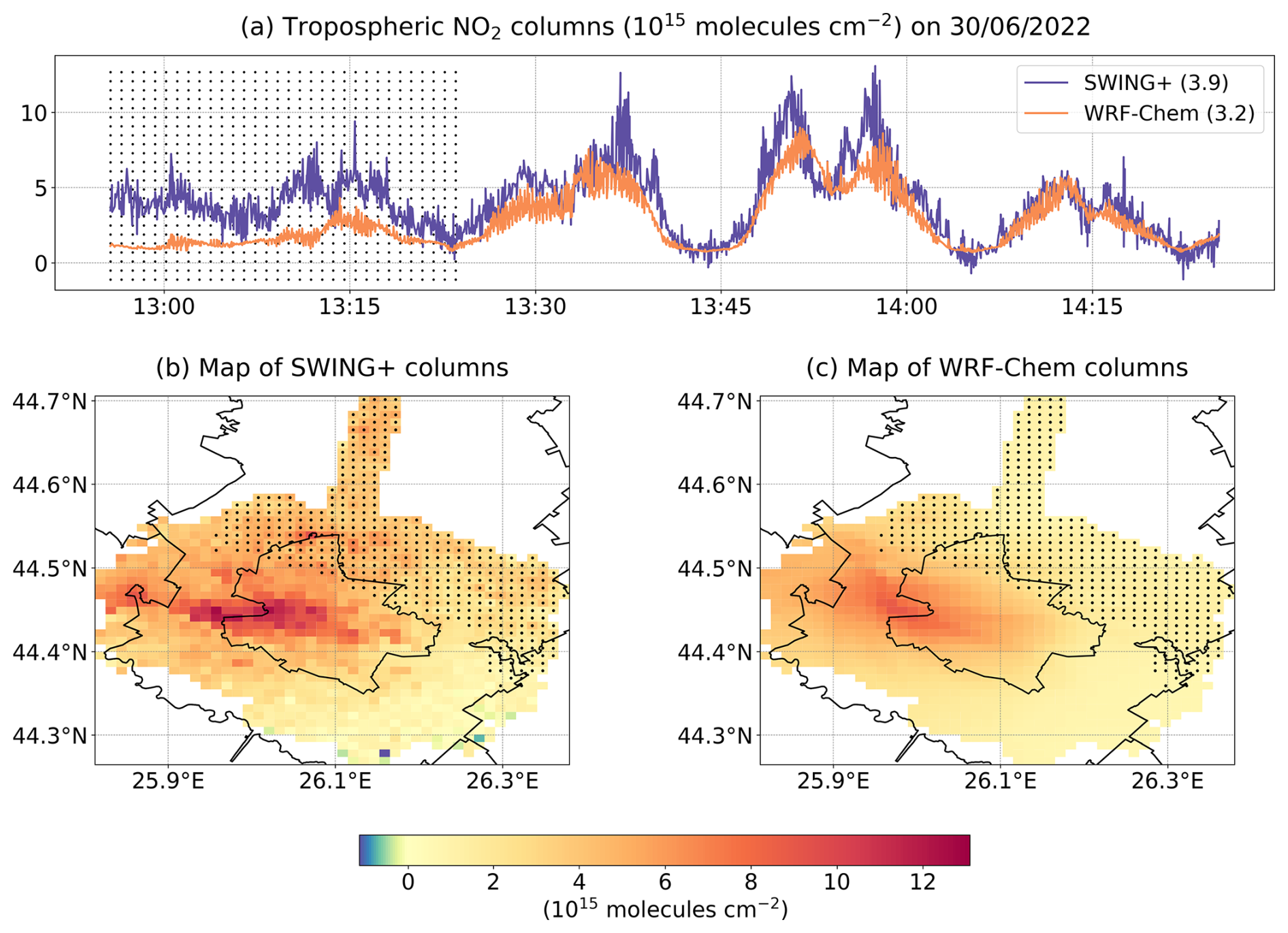
Figure 8 Tropospheric NO₂ columns on Thursday 30 June 2022, presented as a temporal series of SWING+ and WRF-Chem values plotted against local time, with mean values in parentheses in (a), and corresponding maps in (b) and (c). Dotted values, acquired from 12:55 to 13:24 LT, are excluded from the analysis for reasons explained in the text.

Thereafter, the modeled columns correlate very well with the measurements, with a Pearson's coefficient of 0.89. This time, however, the model tends to underestimate the measurements, with a small RB of −18 % and an error of 1.5×10¹⁵ molec. cm⁻². This latter metrics is dominated by small columns associated with the background, where the model slightly overestimates the measurements, similarly to what was found for 11 November 2021, though to a lesser extent.

3.2.3 Summary for all flights

Table 6 presents the evaluation of NO₂ columns from WRF-Chem against SWING+ measurements using the statistical metrics from Table 4, for each separate flight. It also provides statistics per season and for the entire dataset. For two dates, namely 10 July 2021 and 30 June 2022, we truncate data associated with the beginning of the flight for reasons explained in Sect. 3.2.2. Inspection of both datasets, conducted independently of each other, indicated that selecting 13:24 LT as the start time was appropriate, instead of the time reported in Table 1. In Sect. S3, Table S4 provides the comparison statistics (similar to Table 6) for runs with and without the factor of 1.5 applied to CAMS-REG v7.0 NO_x emissions. Equivalents of Figs. 7 and 8 for the other flight dates, simulated with upscaled emissions, are presented in Sect. S4.

Table 6 Evaluation of tropospheric NO₂ columns from WRF-Chem against SWING+ measurements, regridded to the resolution of the model, for each flight day. For dates marked with a dagger (†), measurements have been truncated to start at the time of 13:24 LT. The last rows assembles data by season or for all dates combined, excluding the worst-performing one, 22 November 2021, when marked with an asterisk (*).

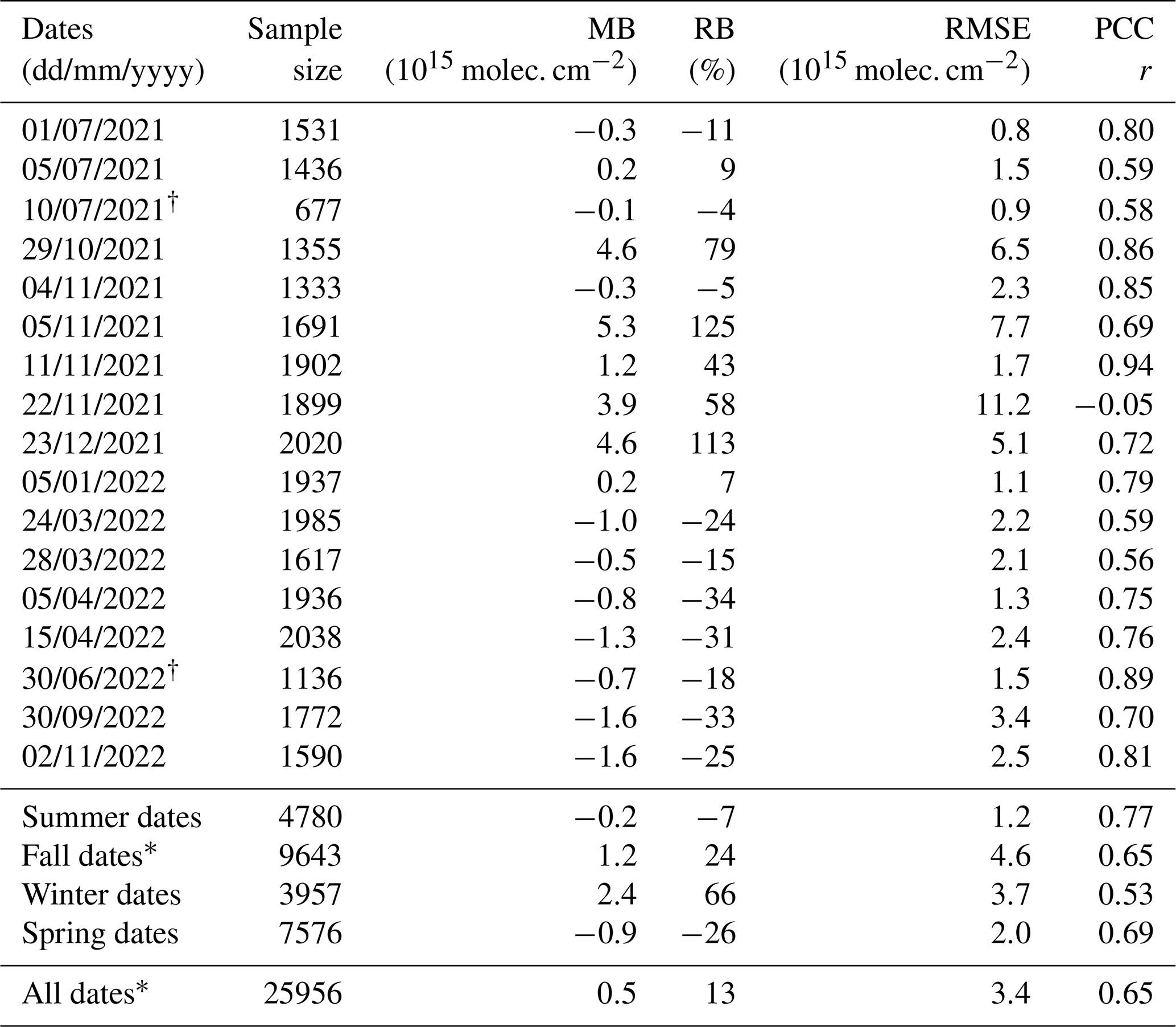
The specific case of 22 November 2021 stands out as an outlier due to its large RMSE (11.2×10¹⁵ molec. cm⁻²) and a correlation coefficient close to 0 (−0.05). A detailed inspection of the model meteorological performance for that day, in comparison with ANM measurements, reveals that it fails to accurately reproduce a change in surface wind direction just before SWING+ begins recording. The observations indicate a transition from westerly to easterly winds occurring between 05:00 and 09:00 LT. In contrast, the model simulates this transition beginning around 08:00 and completing near 13:00, resulting in a delay of approximately three to four hours. This issue justifies the omission of this flight from further analyses.

The comparable numbers of days with either positive (7) or negative (10) biases in Table 6 suggest a balanced model behavior on average. The small overall bias across all selected dates (MB of 0.5×10¹⁵ molec. cm⁻² and RB of 13 %), along with the underestimation in surface ${\mathrm{NO}}_{\mathrm{2}}^{*}$ found in Sect. 2.2.2 (MB of −8 µg m⁻³ and RB of −33 %), provides a retrospective justification for increasing the CAMS-REG anthropogenic NO_x emissions by a factor of 1.5, as proposed in Sect. 2.1.2.

The small overall model bias against SWING+ reflects compensating seasonal biases of opposite sign, indicating that a temporally varying scaling factor for NO_x emissions may be more realistic. However, while finer, day-specific adjustments based on the column evaluations in Table 6 could be considered, they would likely introduce abrupt and potentially unrealistic temporal variations in emissions, e.g., in November 2021, when the mean model bias ranges from −5 % to +125 % across different days. This variability may reflect the fact that, in addition to emission uncertainties, the model daily performance (e.g., chemistry and transport) on a limited set of days can strongly influence seasonal statistics, particularly in winter and fall, whereas spring and summer appear more consistent.

The RMSE exceeds 5×10¹⁵ molec. cm⁻² on only three of the selected dates and remains at or below 2.5×10¹⁵ molec. cm⁻² for 12 dates. The RB lies within ±50 % for 13 dates, and within ±25 % for 9 dates, making them comparable to the results obtained by Poraicu et al. (2023). Correlation coefficients range from 0.56 to 0.94, with 10 dates above 0.75 and a satisfactory overall value of 0.65 for the compilation of all selected dates.

The seasonal statistics in Table 6 show an underestimation of NO₂ columns during summer and spring, and an overestimation during winter and fall. The model underestimation in summer and spring is consistent with the underestimation of the observed surface concentrations during daytime (Sect. 3.1.2). These discrepancies may result from emission errors, inaccuracies in vertical mixing and/or oxidant levels, and possibly issues related to other model species. The surface measurements indicated a close agreement with the model during the first hours of daytime in fall and an overestimation in winter before the underestimation sets in (see Fig. 6). This does not appear in the comparison with SWING+ data in Table  6. One possible explanation is that the model lifts NO₂ species too far from the surface, at altitudes where SWING+ is more sensitive.

3.3 TROPOMI validation

3.3.1 Correcting WRF-Chem bias using SWING+

We first compare SWING+ measurements Ω_S with WRF-Chem outputs Ω_W,S, accounting for SWING+ averaging kernels and acquisition times, but this time at TROPOMI spatial resolution. Specifically, we use a linear regression, denoted by LR₁, to predict the SWING+ column value from a given WRF-Chem column Ω_W,S, as defined in Eq. (4):

$$\begin{array}{}\text{(6)}& {\text{LR}}_{\mathrm{1}}\left({\mathrm{\Omega }}_{\text{W},\text{S}}\right)={\mathit{\alpha }}_{\mathrm{0}}+{\mathit{\alpha }}_{\mathrm{1}}{\mathrm{\Omega }}_{\text{W},\text{S}},\end{array}$$

where α₀ and α₁ are scalar values to be determined through separate linear regressions for each flight day. This is because the comparisons of WRF-Chem with SWING+ data show significant variations across different flight dates. Additionally, we exclude the flight of 22 November 2021 from the present analysis due to the lack of correlation between the model and the flight data (cf. Sect. 3.2).

We adopt the Theil–Sen estimator (Theil, 1950; Sen, 1968) for all selected dates (implemented via scipy.theilslopes along with a custom code to bootstrap the associated uncertainties). This method offers greater robustness to outliers and improved accuracy in error estimation compared to parametric methods such as ordinary and weighted least squares (Wilcox, 2010). A comparison of these three methods applied to our datasets is provided in Sect. S5. The results of the Theil–Sen regression for the selected flight dates are shown in Fig. 9. As expected from the results presented in Sect. 3.2, both intercepts and slopes vary significantly across the different flights, along with their associated uncertainties.

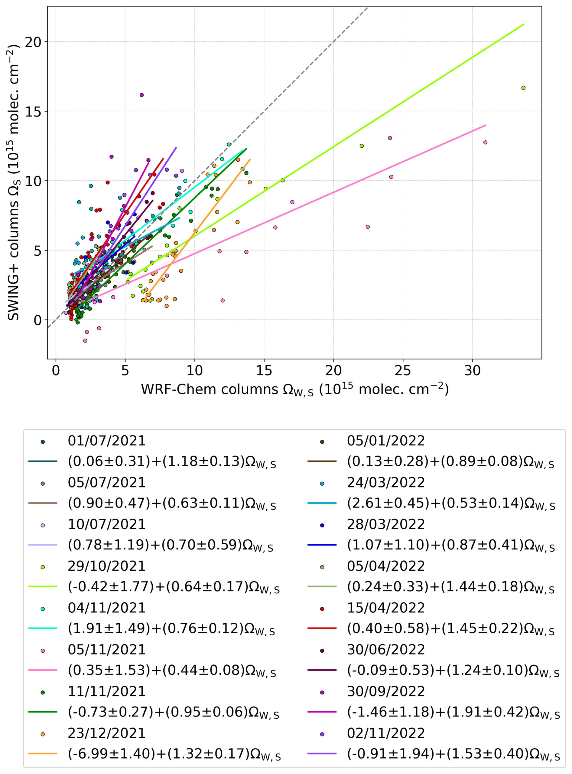
Figure 9 Scatter plot of SWING+ and WRF-Chem column values for our selection of 16 flight days. For each date, Theil–Sen estimators are used to determine the linear relationship LR₁, along with associated uncertainties on the fitted coefficients.

The WRF-Chem tropospheric columns used for comparison with TROPOMI, denoted Ω_W,T, are constructed using TROPOMI averaging kernels and calculated at the satellite acquisition times, as defined in Eq. (5). However, these are likely biased, just like Ω_W,S, so we define a bias-corrected version of the column, ${\mathrm{\Omega }}_{\text{W},\text{T}}^{\text{bc}}$, based on the model evaluation against SWING+ data, as derived in the previous step:

$$\begin{array}{}\text{(7)}& {\mathrm{\Omega }}_{\text{W},\text{T}}^{\text{bc}}={\text{LR}}_{\mathrm{1}}\left({\mathrm{\Omega }}_{\text{W},\text{T}}\right)={\mathit{\alpha }}_{\mathrm{0}}+{\mathit{\alpha }}_{\mathrm{1}}{\mathrm{\Omega }}_{\text{W},\text{T}}.\end{array}$$

These bias-corrected columns can then be directly compared to the TROPOMI measurements, Ω_T, since they are evaluated at the same time and account for TROPOMI vertical sensitivity through the term α₁Ω_W,T. Note that the constant term, α₀, was evaluated while accounting for SWING+ vertical sensitivity. However, correcting this term is not feasible without additional knowledge of the true atmospheric vertical profile. Nevertheless, its contribution to the overall expression is expected to be minor, as explained in Appendix A.

3.3.2 Evaluation of TROPOMI bias

By combining datasets from different flight days, either collectively or by season, we can assess the TROPOMI columns Ω_T against the bias-corrected WRF-Chem columns ${\mathrm{\Omega }}_{\text{W},\text{T}}^{\text{bc}}$, using a linear regression denoted by LR₂:

$$\begin{array}{}\text{(8)}& {\text{LR}}_{\mathrm{2}}\left({\mathrm{\Omega }}_{\text{W},\text{T}}^{\text{bc}}\right)={\mathit{\beta }}_{\mathrm{0}}+{\mathit{\beta }}_{\mathrm{1}}{\mathrm{\Omega }}_{\text{W},\text{T}}^{\text{bc}},\end{array}$$

where β₀ and β₁ are scalar parameters. Unlike in Sect. 3.3.1, this linear regression involves two datasets that both contain random errors. TROPOMI measurements are affected by instrument precision, with an average uncertainty of ${\mathit{\sigma }}_{\text{T}}=\mathrm{1.3}\times {\mathrm{10}}^{\mathrm{15}}$ molec. cm⁻² across all selected dates. The average uncertainty of the bias-corrected dataset is limited by the precision of the regression method used to produce it and is estimated at ${\mathit{\sigma }}_{{\text{LR}}_{\mathrm{1}}}=\mathrm{0.5}\times {\mathrm{10}}^{\mathrm{15}}$ molec. cm⁻².

Because most of the random uncertainty is due to the TROPOMI columns,² the Theil–Sen estimator remains applicable in this context. We compare this approach to other parametric alternatives in Sect. S5. Among them, the orthogonal distance regression with weights (implemented via scipy.ODRPACK,  Boggs et al., 1992) accounts explicitly for errors on both axes, together with possible heterogeneity (heteroscedasticity). As shown in Sect. S5, it produces similar regression results to the Theil–Sen method and performs slightly better in terms of mean absolute deviation of the fit. We interpret this result as evidence that outliers do not significantly influence the orthogonal regression. Therefore, we choose this parametric method based on its better fit performance, while noting that both approaches yield consistent results and thus reinforce each other. The resulting scatter plot is shown in Fig. 10.

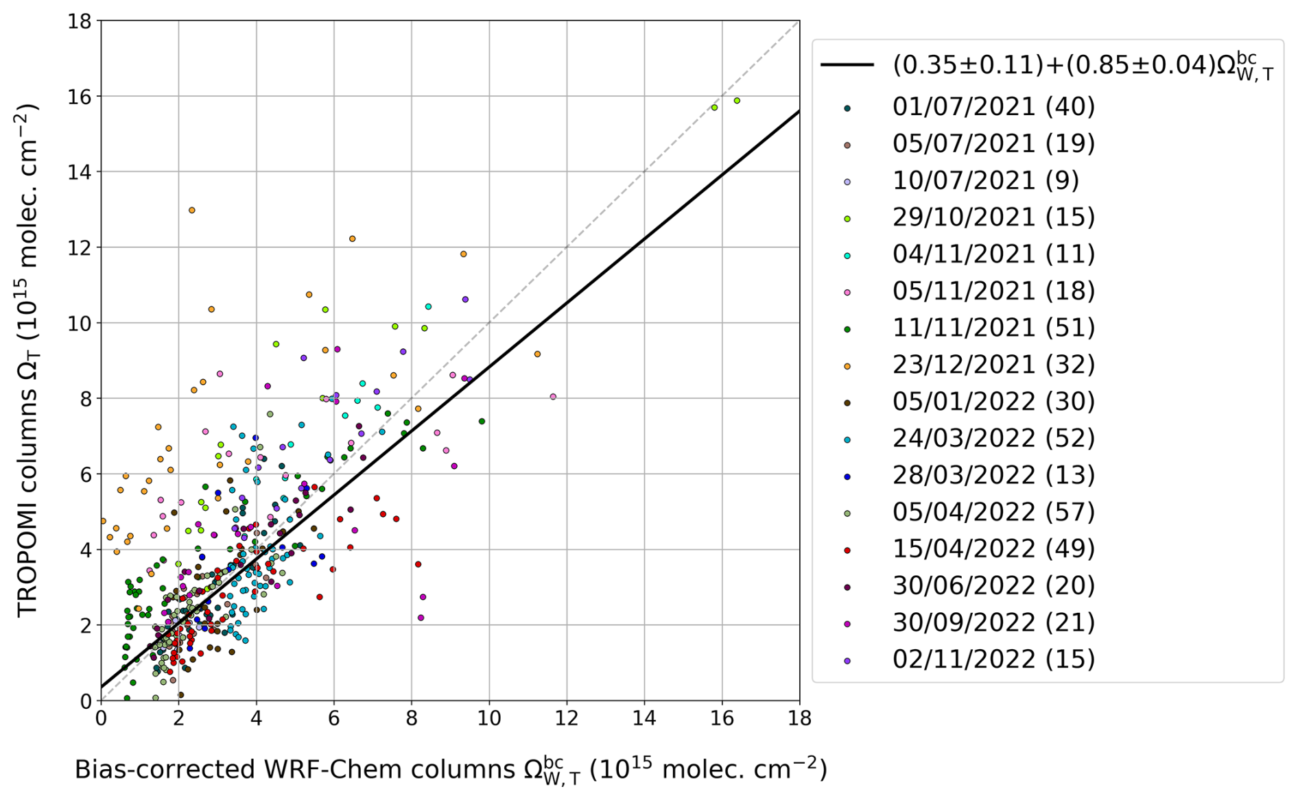
Figure 10 Scatter plot of 452 TROPOMI and bias-corrected WRF-Chem column values for all flight days (except 22 November 2021). Weighted orthogonal distance regression estimators are used to determine the linear relationship LR₂, along with associated uncertainties on the fitted coefficients. For each date, the number of columns is displayed in parentheses.

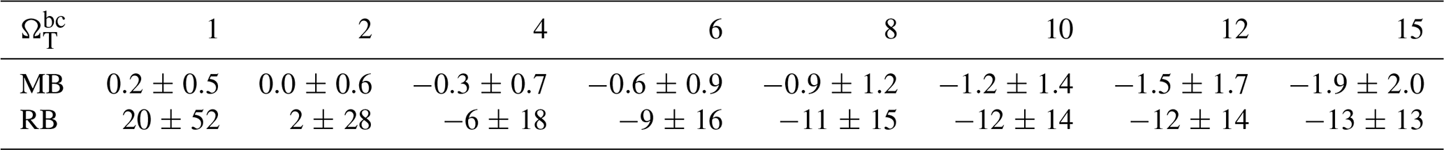
For different values of the bias-corrected column ${\mathrm{\Omega }}_{\text{T}}^{\text{bc}}$ in the range $(\mathrm{1}-\mathrm{15})\times {\mathrm{10}}^{\mathrm{15}}$ molec. cm⁻², the regression line LR₂ allows to estimate the bias in TROPOMI measurements:

$$\begin{array}{}\text{(9)}& {\mathrm{\Omega }}_{\text{T}}-{\mathrm{\Omega }}_{\text{T}}^{\text{bc}}={\text{LR}}_{\mathrm{2}}\left({\mathrm{\Omega }}_{\text{T}}^{\text{bc}}\right)-{\mathrm{\Omega }}_{\text{T}}^{\text{bc}}={\mathit{\beta }}_{\mathrm{0}}+({\mathit{\beta }}_{\mathrm{1}}-\mathrm{1}){\mathrm{\Omega }}_{\text{T}}^{\text{bc}}\pm {\mathit{\sigma }}_{\text{b}}.\end{array}$$

Before substituting numerical values into this expression, we first summarize the sources of uncertainty that contribute to the bias estimation, captured in σ_b.

The bias-corrected WRF-Chem columns ${\mathrm{\Omega }}_{\text{W},\text{T}}^{\text{bc}}$ carry the random uncertainty of the SWING+ columns σ_S,rand because LR1 propagates it through the regression. This random error is therefore reflected in the uncertainties of LR₂, as displayed in the legend of Fig. 10. However, the systematic component of the SWING+ measurement error, denoted σ_S,syst, was not included. We incorporate it now into the evaluation of TROPOMI bias, in addition to the random uncertainty already present from the evaluation of the regression LR₂, denoted as ${\mathit{\sigma }}_{{\text{LR}}_{\mathrm{2}}}$:

$$\begin{array}{}\text{(10)}& {\mathit{\sigma }}_{\text{b}}=\sqrt{{\mathit{\sigma }}_{{\text{LR}}_{\mathrm{2}}}^{\mathrm{2}}+{\mathit{\beta }}_{\mathrm{1}}^{\mathrm{2}}{\mathit{\sigma }}_{\text{S},\text{syst.}}^{\mathrm{2}}}.\end{array}$$

The uncertainty ${\mathit{\sigma }}_{{\text{LR}}_{\mathrm{2}}}$ is determined from the uncertainties in the regression parameters β₀ and β₁, whereas σ_S,syst arises from uncertainties associated with the reference slant column and the air mass factors used in the computation of the SWING+ vertical column density (Sect. 2.2.3). The error in the residual slant column is indeed purely systematic, and for simplicity, the AMF uncertainty is likewise assumed to be systematic, without a random component. Finally, we express the main result of this section as:

$$\begin{array}{}\text{(11)}& \begin{array}{rl}{\mathrm{\Omega }}_{\text{T}}-{\mathrm{\Omega }}_{\text{T}}^{\text{bc}}& =\mathrm{0.35}-\mathrm{0.15}{\mathrm{\Omega }}_{\text{T}}^{\text{bc}}\\ & \pm \sqrt{(\mathrm{0.51}{)}^{\mathrm{2}}-\mathrm{0.01}{\mathrm{\Omega }}_{\text{T}}^{\text{bc}}+(\mathrm{0.13}{\mathrm{\Omega }}_{\text{T}}^{\text{bc}}{)}^{\mathrm{2}}},\end{array}\end{array}$$

with ${\mathrm{\Omega }}_{\text{T}}^{\text{bc}}$ in units of 10¹⁵ molec. cm⁻². Bias estimates for various column values ${\mathrm{\Omega }}_{\text{T}}^{\text{bc}}$ are presented in Table 7. Details on how to obtain the numerical expression for the error from Eq. (10) are provided in Appendix B.

Table 7 TROPOMI mean biases, $\text{MB}={\mathrm{\Omega }}_{\text{T}}-{\mathrm{\Omega }}_{\text{T}}^{\text{bc}}$ (10¹⁵ molec. cm⁻²), and relative biases, $\text{RB}=({\mathrm{\Omega }}_{\text{T}}-{\mathrm{\Omega }}_{\text{T}}^{\text{bc}})/{\mathrm{\Omega }}_{\text{T}}^{\text{bc}}$ (%), for various column values ${\mathrm{\Omega }}_{\text{T}}^{\text{bc}}$ (10¹⁵ molec. cm⁻²) within the range of applicability of our results, roughly $(\mathrm{1}-\mathrm{15})\times {\mathrm{10}}^{\mathrm{15}}$ molec. cm⁻².

We can further invert the linear relation LR₂ to estimate a bias-corrected column ${\mathrm{\Omega }}_{\text{T}}^{\text{bc}}$ for a given TROPOMI measurement Ω_T, in 10¹⁵ molec. cm⁻²:

$$\begin{array}{}\text{(12)}& \begin{array}{rl}{\mathrm{\Omega }}_{\text{T}}^{\text{bc}}& =-\mathrm{0.42}+\mathrm{1.18}{\mathrm{\Omega }}_{\text{T}}\\ & \pm \sqrt{(\mathrm{0.61}{)}^{\mathrm{2}}-\mathrm{0.04}{\mathrm{\Omega }}_{\text{T}}+(\mathrm{0.19}{\mathrm{\Omega }}_{\text{T}}{)}^{\mathrm{2}}}.\end{array}\end{array}$$

Similar to the previous expression, the uncertainty has been calculated to account for the systematic error in the SWING+ product, in addition to the uncertainty arising from the precision of the linear regression method.

We reproduce the linear regression for the selected dates grouped by season in Fig. 11. Our first remark is that the results for winter are of lower quality than in other seasons, due to the small size of the dataset, which covers only two dates (23 December 2021 and 5 January 2022) for a total of 62 columns. The flight day of 23 December 2021 shows less convincing results (Table 6) and is characterized by consistently high modeled background values (see Sect. S4), which may be due to inaccurate initial or boundary conditions for NO_x, oxidant concentrations, and/or heterogeneous chemistry on aerosols. When focusing on the most reliable of the two dates, 5 January 2022, we find that the resulting fit matches well the general relationship of Fig. 10. Therefore, we consider this date alone to provide a more robust basis for the winter analysis presented in the next paragraph. Note that excluding 23 December 2021 from the general analysis in Fig. 10 does not significantly affect the result. The resulting regression line becomes $(\mathrm{0.21}\pm \mathrm{0.10})+(\mathrm{0.87}\pm \mathrm{0.04}){\mathrm{\Omega }}_{\text{W},\text{T}}^{\text{bc}}$, which remains consistent with the original fit within the estimated uncertainties.

Remarkably, the summer scatter plot shows very little bias, with a value of $-\mathrm{0.1}\times {\mathrm{10}}^{\mathrm{15}}$ molec. cm⁻², and no apparent dependence on the column value. Taking into account SWING+ systematic errors, at low column densities of 2 × 10¹⁵ molec. cm⁻², we find relative biases of $-\mathrm{6}\pm \mathrm{25}\mathit{\%}$ (summer), 50 ± 38 % (fall), $-\mathrm{15}\pm \mathrm{44}\mathit{\%}$ (winter), and $-\mathrm{14}\pm \mathrm{24}\mathit{\%}$ (spring). For high column values of 10¹⁶ molec. cm⁻² (even though this is slightly outside the range of applicability for summer, winter, and spring), we estimate the relative biases to be $-\mathrm{1}\pm \mathrm{17}\mathit{\%}$ (summer), 0 ± 16 % (fall), $-\mathrm{15}\pm \mathrm{29}\mathit{\%}$ (winter), and $-\mathrm{18}\pm \mathrm{14}\mathit{\%}$ (spring).

Due to partial cloudiness on 4 flight dates (5 July 2021, 5 November 2021, 23 December 2021, and 15 April 2022), a sensitivity analysis was performed by repeating the analysis shown in Figs. 10 and 11, excluding these dates (Sect. S5). Only minor differences are observed, except in winter, which has already been discussed.

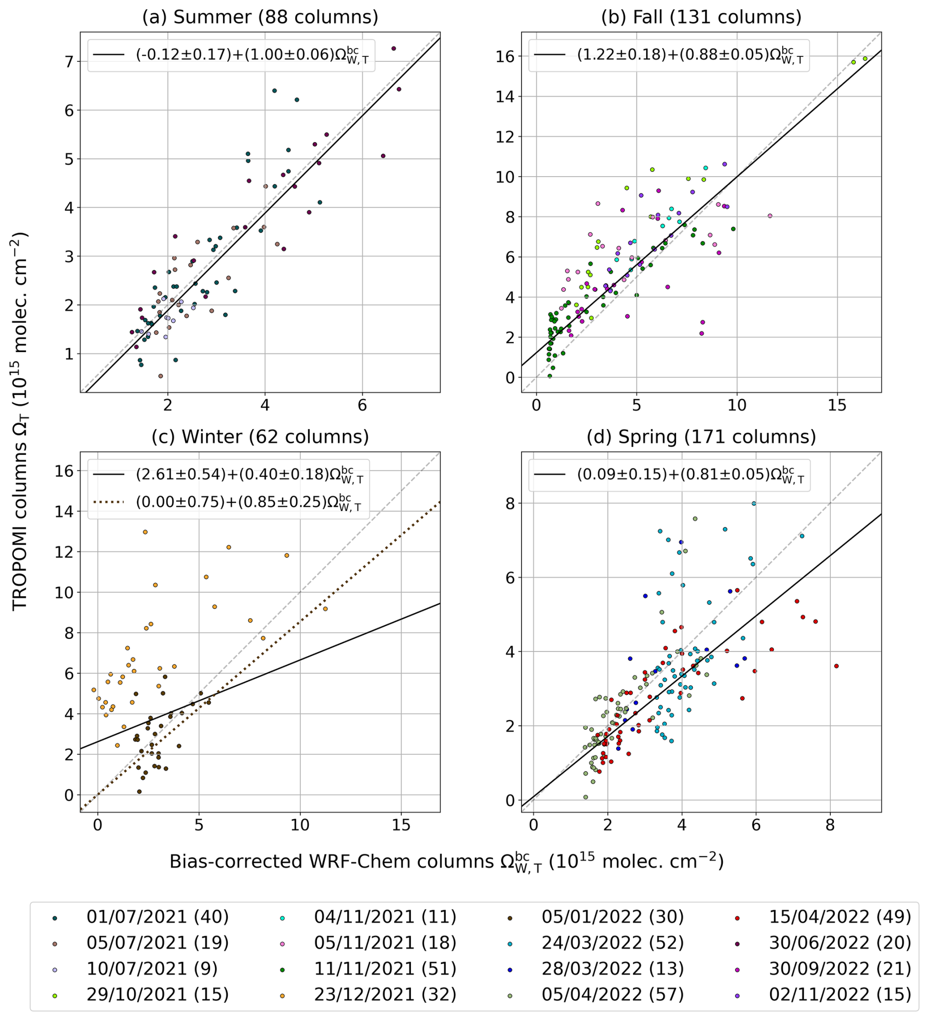
Figure 11 Seasonal scatter plots of TROPOMI versus bias-corrected WRF-Chem column values for the selected flight days: (a) summer, (b) fall, (c) winter, and (d) spring. Weighted orthogonal distance regression estimators are used to determine the seasonal linear relationships (solid lines), as well as the day-specific regression for 5 January 2022 during winter (dotted line), including the associated uncertainties on the fitted coefficients. For each time period, the number of columns is displayed in parentheses.

4 Review of TROPOMI tropospheric NO₂ validation

Tables 8 and 9 summarize literature results on the validation of TROPOMI tropospheric NO₂ products. The studies span from 2019 to 2025, cover several TROPOMI product versions, and focus primarily on populated regions in North America, Europe, and China, while also including less-studied environments such as Kinshasa (Yombo Phaka et al., 2023). Table 8 compiles results from studies that employed Pandora column measurements from the Pandonia Global Network (Herman et al., 2009) and MAX-DOAS instruments (Hönninger et al., 2004), while Table 9 presents comparisons with airborne measurements, including our own results using SWING+. Overall, the reported relative biases are predominantly negative across both low and high column abundances. Most biases fall within the ±50 % acceptance range set by TROPOMI requirements (van Geffen et al., 2024). Note that, compared to the previous section, we have reduced the column concentration range by raising the lower bound from 10¹⁵ to 4×10¹⁵ molec. cm⁻², with an upper bound placed at 15×10¹⁵ molec. cm⁻². This adjustment reflects the fact that most of the referenced studies were conducted in polluted urban environments, typically more polluted than Bucharest and its surrounding rural regions, with NO₂ columns generally much higher than 10¹⁵ molec. cm⁻². Results from Chan et al. (2020), Verhoelst et al. (2021), and Lambert et al. (2025), which do not fit our table format, are discussed separately below.

Griffin et al. (2019)Zhao et al. (2020)Judd et al. (2020)Douros et al. (2023)Dimitropoulou et al. (2020)Cai et al. (2022)van Geffen et al. (2022)Douros et al. (2023)Yombo Phaka et al. (2023)

Table 8 Compilation of past studies evaluating TROPOMI tropospheric NO₂ against reference columns: Ω_P (Pandora) and Ω_MD (MAX-DOAS), in units of 10¹⁵ molec. cm⁻². The validation method used is either a direct comparison (a) or a comparison accounting for recalculated air mass factors (b). From the regressions, percentage relative biases (RB) at low (4 × 10¹⁵ molec. cm⁻²) and high (15 × 10¹⁵ molec. cm⁻²) column values are calculated.

Griffin et al. (2019)Judd et al. (2020)Tack et al. (2021)Lange et al. (2023)Poraicu et al. (2023)Johnson et al. (2023)

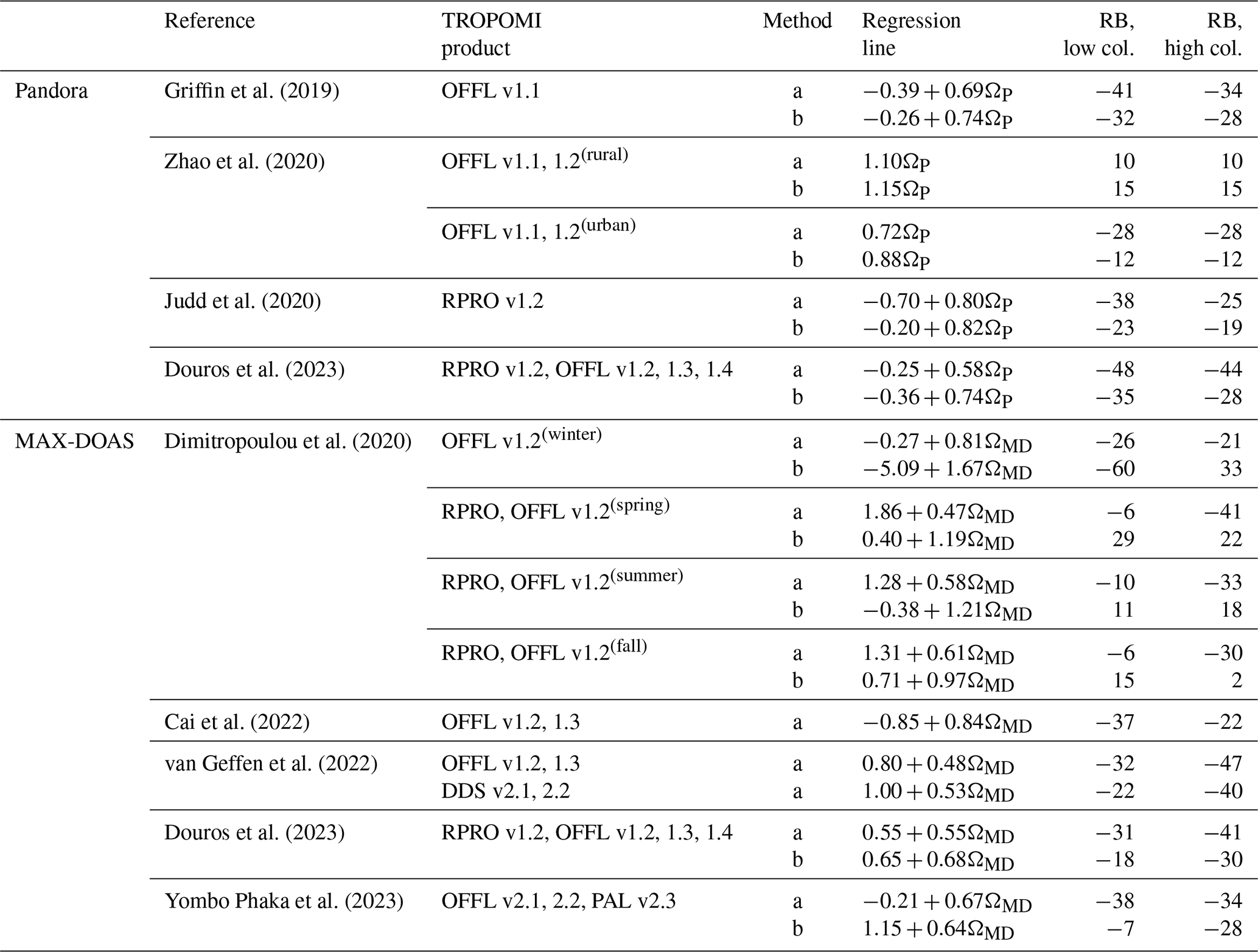
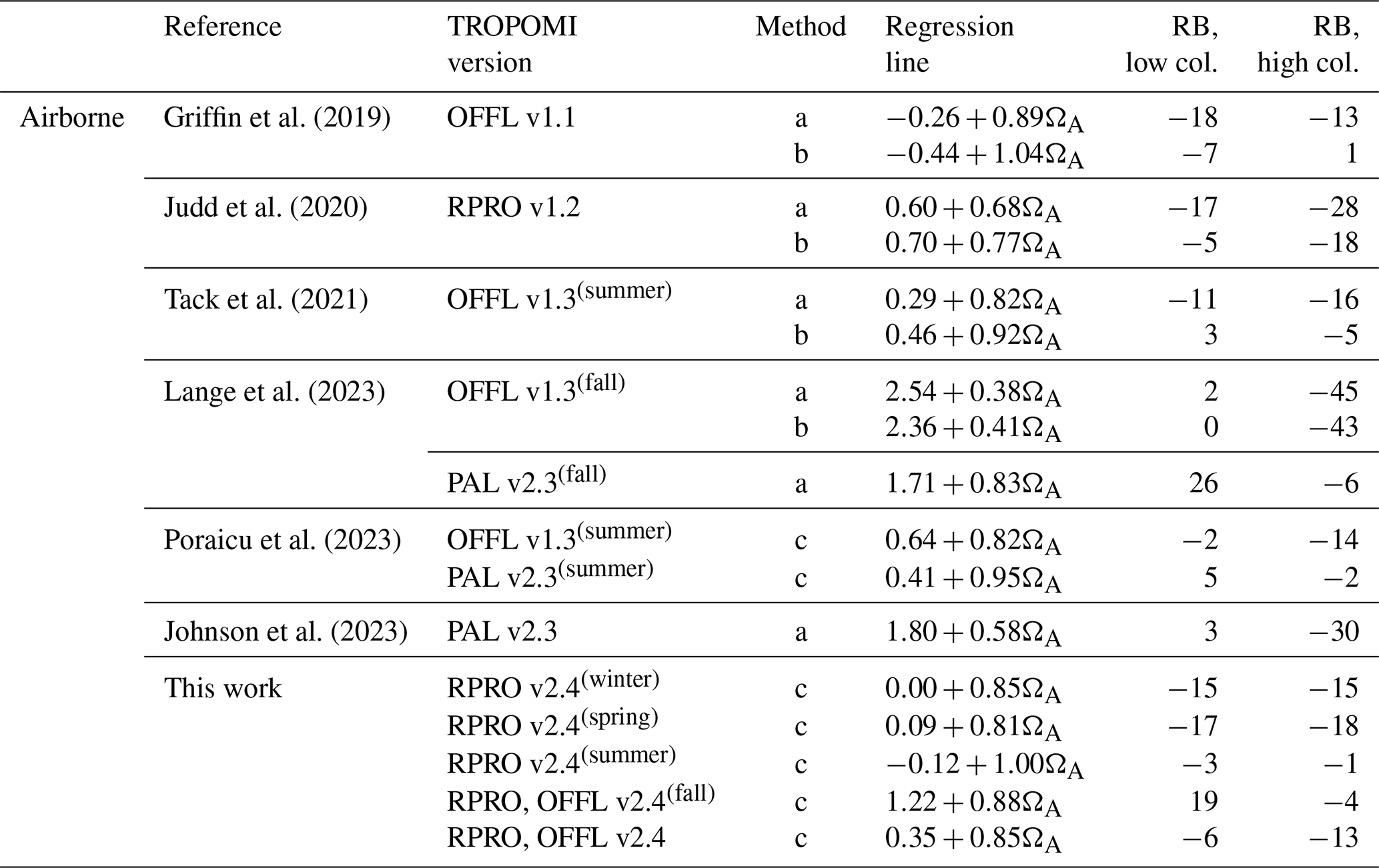
Table 9 Same as for Table 8, except that airborne measurements are used for validation. The validation method used is either a direct comparison (a), a comparison accounting for recalculated air mass factors (b), or denotes the use of WRF-Chem combined with TROPOMI averaging kernels as detailed in Sect. 2 (c).

The reported studies span TROPOMI product versions from v1.1 to v2.8, with Lambert et al. (2025) using v2.4, the version adopted in this work. We summarize the changes following van Geffen et al. (2024), which guides our treatment of the different products. Versions v1.2 and v1.3 introduced only minor refinements with negligible impact on column values with respect to v1.1; we group these together. A major update came with v1.4, which improved the cloud retrieval algorithm and led to higher NO₂ columns, especially in polluted regions. Since Douros et al. (2023) used v1.4 for only four months in a three-year analysis that otherwise relies on products from earlier product versions, we will compare their results with those from the v1.1–1.3 group. Further updates from v2.2 to v2.4 included improvements to the surface albedo, which enhanced radiative closure and reduced low biases in vegetated regions such as the Amazon basin. Versions v2.4 to v2.8 maintained a stable retrieval framework with only minor adjustments. Given the overall consistency of later versions in urban settings, we group versions v2.1 through v2.8 together for comparison.

For v1.1 to v1.3, direct comparisons with Pandora, MAX-DOAS, and airborne measurements, indicate a median bias of −17.5 % for low columns (4 × 10¹⁵ molec. cm⁻²) and −28 % for high columns (15 × 10¹⁵ molec. cm⁻²). These results align with those of Verhoelst et al. (2021), who reported biases ranging from −15 % to −56 % in direct comparisons with MAX-DOAS across multiple sites worldwide. Similarly, Douros et al. (2023), who also analyze the v1.4 product, find negative biases for both column ranges, with biases ranging from −31 % to −48 % for both Pandora and MAX-DOAS comparisons.

Several studies recalculated the air mass factor (AMF) for versions v1.1 to v1.4 using alternative a priori profiles in place of those from the TM5-MP model (Williams et al., 2017). For example, Griffin et al. (2019) and Zhao et al. (2020) used GEM-MACH profiles (Moran et al., 2010; Pendlebury et al., 2018); Judd et al. (2020) used NAMCMAQ (Stajner et al., 2011); and Tack et al. (2021); Douros et al. (2023); Lange et al. (2023) used CAMS profiles (Colette et al., 2025). In addition, Chan et al. (2020) and Dimitropoulou et al. (2020) employed vertical profiles derived directly from MAX-DOAS observations. These adjustments generally lead to less negative, or more positive biases. For low columns, the median bias across these studies is −6 %, and for high columns, −11.5 %. Chan et al. (2020) also noted that improving the AMF reduced the bias by up to 17 %. In most of the reported studies, recalculating the AMF reduces the bias, with reductions of 6 % to 20 % observed in half of the cases.

The same aircraft campaign and TROPOMI product version (v1.3) were used by Tack et al. (2021) and Poraicu et al. (2023). Tack et al. (2021) reported results based on direct comparisons and using CAMS-based AMFs, while Poraicu et al. (2023) aligned with our approach, employing the WRF-Chem model as an intercomparison platform and incorporating TROPOMI averaging kernels. The improvement relative to direct comparison is more pronounced when CAMS-based AMFs are used. Specifically, applying CAMS AMFs and the model-based method reduces the low-column bias from −11 % to 3 % and −2 %, respectively. For high columns, the bias improves from −16 % to −5 % and −14 %.

We now turn to the evaluation of TROPOMI products v2.1 to v2.8. Median biases reported in Table 8 for direct comparisons relative to MAX-DOAS are −30 % for low columns and −37 % for high columns. These values closely match those reported by Lambert et al. (2025): −29 % for polluted stations (3 to 14 × 10¹⁵ molec. cm⁻²) and −38 % for extremely polluted stations ($>\mathrm{15}\times {\mathrm{10}}^{\mathrm{15}}$ molec. cm⁻²). Yombo Phaka et al. (2023) recalculated TROPOMI columns using vertical profiles derived from MAX-DOAS measurements and found a bias reduction of 31 % and 6 % of low and high columns, respectively. Similarly, Lambert et al. (2025) noted that applying TROPOMI averaging kernels to MAX-DOAS vertical profiles leads to a bias reduction by up to 20 %.

Direct comparisons with aircraft campaigns indicate that biases for high columns have decreased with newer TROPOMI product versions. Using version v1.3, median biases are −14 % for low columns and −22 % for high columns. In contrast, for more recent versions (v2.3), we find similar low-column biases (−14.5 %), but improved performance for high columns, with a median bias of −18 %. This suggests that product upgrades have slightly improved performance in polluted conditions. However, incorporating WRF-Chem and TROPOMI averaging kernels has a stronger impact, reducing the biases in version v2.3 to 5 % and −2 % for low and high column values, respectively, as shown by Poraicu et al. (2023). Our summertime results using v2.4 are similar, with very small biases for low and high columns (Table 9). Considering all seasons, overall biases are −6 % for low columns and −13 % for high columns in our work.

Finally, we assess the seasonal dependence of the TROPOMI bias. In our study, low-column biases range from −17 % to 19 % across seasons, while high-column biases range from −1 % to −18 %. Our summer results (−3 % and −1 % for low and high columns, respectively) agree well with the aircraft-based analysis for the PAL v2.3 product of Poraicu et al. (2023), with differences of 8 % or less. Our fall results (19 % and −4 %) are consistent with those of Dimitropoulou et al. (2020) using recalculated AMF, with differences within 6 %. They are also in line with Lange et al. (2023), showing positive biases for low columns. However, for high columns in fall, both our study and Lange et al. (2023) report negative biases, a feature captured by Dimitropoulou et al. (2020) only when using the original AMF. In contrast, winter and spring results show weaker consistency with Dimitropoulou et al. (2020). However, differences in methodology (notably the use of dual-scan MAX-DOAS observations) and in the TROPOMI product version limit direct comparability. This underscores the need for further validation studies, particularly in winter and spring, where comparable aircraft campaigns are lacking.

5 Conclusions

This study presents an evaluation of tropospheric NO₂ over Bucharest, combining high-resolution WRF-Chem simulations with multiple observational datasets. We assess the WRF-Chem performance against in situ meteorological and surface concentration measurements, as well as airborne column observations from SWING+, while independently validating TROPOMI tropospheric NO₂ products using a model-based intercomparison framework. This joint analysis provides insight into both the modeling capabilities and satellite product validity over a complex and understudied urban environment.

Comparison against surface meteorological variables shows that WRF-Chem reproduces key features of regional meteorology. Across 17 two-day periods, surface pressure, temperature, relative humidity, and solar radiation are well represented, with mean biases within 1 mbar, 0.5 °C, 6 %, and 37 W m⁻², respectively. Temporal correlation coefficients are higher than 0.95 for pressure, temperature, and radiation, and higher than 0.85 for relative humidity. Wind speed exhibits a positive bias of 1.0 m s⁻¹, consistent with previous WRF-Chem studies (Kim et al., 2013; Feng et al., 2016; Poraicu et al., 2023), while wind direction shows a mean bias below 16°. The temporal correlation for the horizontal wind vector is generally weaker (r=0.64). On 22 November 2021, a mismatch in wind direction appeared to negatively impact the modeled NO₂ column evaluation. Aside from this case, the model successfully captures the meteorological conditions required to support atmospheric chemistry assessments, using a common configuration and set of parameterizations.

Modeled surface concentrations of NO and NO₂ exhibit consistent daytime underestimations, concomitant with an overestimation of O₃. When restricting the comparison to non-traffic sites, the mean bias remains within −8 µg m⁻³ for both NO and NO₂, accounting for potential interference from NO_y reservoir species. Temporal correlations exceed 0.70 for NO and NO₂, and reach 0.81 for O₃, successfully capturing the diurnal and seasonal cycles of all three species. This agreement is improved for NO and NO₂ during colder months, and for O₃ during warmer periods.

WRF-Chem performs generally well against airborne SWING+ measurements of the tropospheric NO₂ column. Across 16 selected flight days, it exhibits a mean bias of 0.5 × 10¹⁵ molec. cm⁻² (13%), with correlation coefficients exceeding 0.75 in 9 cases. Seasonal patterns emerge: summer and spring flights show model underestimation of −7 % and −26 %, respectively, while fall and winter show positive biases of 24 % and 66 %. The spring and summer underestimations of NO₂ columns are reminiscent of the surface underestimations observed during flight hours. However, a discrepancy arises in fall and winter, as the surface and SWING+ instruments exhibit opposite biases. Finally, we point to model improvements that could help reconcile surface and column levels, beyond correcting the emission inventory, and should be evaluated using more observational data. In particular, vertical mixing (especially in fall and winter) and processes affecting oxidant levels (e.g., volatile organic compounds and their photochemical oxidation) will require further attention.

The underestimation of WRF-Chem NO and NO₂ daytime surface levels, along with the small positive bias for NO₂ modeled column magnitudes across different flight dates, supports an empirical upscaling of CAMS-REG v7.0 anthropogenic NO_x emissions over Bucharest. It is also consistent with the documented low bias in CAMS-REG road-traffic NO_x emissions in European cities with respect to independent urban inventories, estimated at approximately −35 % (Hohenberger et al., 2025). The factor of 1.5 was sufficient for our purpose of validating TROPOMI. However, for a more in-depth assessment of the CAMS-REG inventory, different temporal profiles could be tested (e.g., Guevara et al., 2021), and the overall magnitude could be adjusted seasonally using mass-balance inversion techniques (e.g., Cooper et al., 2017; Poraicu et al., 2023).

TROPOMI tropospheric NO₂ columns v2.4.0 (RPRO + OFFL) are validated using bias-corrected model columns, with SWING+ serving as the reference and TROPOMI averaging kernels applied to the model profiles. The linear relationship expressing the original TROPOMI column, Ω_T, in terms of its bias-corrected counterpart, ${\mathrm{\Omega }}_{\text{T}}^{\text{bc}}$, is given by ${\mathrm{\Omega }}_{\text{T}}=\mathrm{0.35}+\mathrm{0.85}{\mathrm{\Omega }}_{\text{T}}^{\text{bc}}$, in units of 10¹⁵ molec. cm⁻². Relative biases vary with column magnitude, ranging from 20 % at 10¹⁵ molec. cm⁻² to −13 % at 15 × 10¹⁵ molec. cm⁻². A careful treatment of uncertainties from SWING+ observations and the regression method shows that relative bias errors are large at low column values (approximately 50 %), but decrease to within 20 % for columns above 4 × 10¹⁵ molec. cm⁻² and within 15 % for columns exceeding 8 × 10¹⁵ molec. cm⁻². Seasonal analysis reveals greater variability in biases at the low column values (2 × 10¹⁵ molec. cm⁻²), ranging from −15 % in winter to 50 % in fall. In contrast, higher column values (10¹⁶ molec. cm⁻²) exhibit more consistent negative biases, ranging from −18 % in spring to 0 % in fall.

Overall, our results are in agreement with findings from other validation studies in the literature, particularly when considering the associated uncertainties and the methodology employed. Our literature review, focusing on studies over polluted areas, indicates that reported TROPOMI biases for tropospheric NO₂ columns are predominantly negative. For example, median biases range between −30 % and −37 % for NO₂ tropospheric columns of 4–15 ×10¹⁵ molec. cm⁻² across studies using similar TROPOMI product versions (v2.1–v2.3). Good agreement is found with seasonal studies comparing TROPOMI with aircraft (summer) and MAX-DOAS (fall) measurements, with differences relative to our results below 10 %. The scarcity of seasonal studies and the differences in methodology, however, limit the comparability and highlight the need for more dedicated validation campaigns, particularly in winter and spring. This review also underscores that recalculating air mass factors or applying TROPOMI averaging kernels often reduces the biases by approximately 5 % to 20 %, regardless of the version of the TROPOMI products used.

Appendix A: Reference columns and vertical profiles

In Sect. 3.3.1, we introduced the vertical profile n_W modeled with WRF-Chem, where z is the vertical coordinate. We can write a general equation to relate it to the true atmospheric profile, denoted by n:

$$\begin{array}{}\text{(A1)}& n\left(z\right)=\mathit{\delta }n\left(z\right)+\mathit{\alpha }{n}_{\text{W}}\left(z\right),\end{array}$$

where α is an unknown scalar parameter, and δn represents the deviation from linearity. Unlike n and n_W, the function δn may take negative values. At this stage, Eq. (A1) remains too general to be directly informative.

Formally, integrating the profiles n and n_W over the troposphere (Trop), using the airborne instrument averaging kernels A_S, defines the bias-exempt and modeled tropospheric columns, Ω_S and Ω_W,S, respectively:

$$\begin{array}{}\text{(A2)}& {\mathrm{\Omega }}_{\text{S}}=\underset{\text{Trop}}{\int }{A}_{\text{S}}\left(z\right)n\left(z\right)\mathrm{d}z,{\mathrm{\Omega }}_{\text{W},\text{S}}=\underset{\text{Trop}}{\int }{A}_{\text{S}}\left(z\right)n_{\text{W}}\left(z\right)\mathrm{d}z.\end{array}$$

When a linear regression is performed on the datasets Ω_S and Ω_W,S, we estimate the parameters α₀ and α₁ that define the regression line for the estimated values, LR₁:

$$\begin{array}{}\text{(A3)}& {\text{LR}}_{\mathrm{1}}\left({\mathrm{\Omega }}_{\text{W},\text{S}}\right)={\mathit{\alpha }}_{\mathrm{0}}+{\mathit{\alpha }}_{\mathrm{1}}{\mathrm{\Omega }}_{\text{W},\text{S}}.\end{array}$$

These parameters can now be used to constrain Eq. (A1) through the following relations:

$$\begin{array}{}\text{(A4)}& \underset{\text{Trop}}{\int }{A}_{\text{S}}\left(z\right)\mathit{\delta }n\left(z\right)\mathrm{d}z={\mathit{\alpha }}_{\mathrm{0}},\mathit{\alpha }={\mathit{\alpha }}_{\mathrm{1}}.\end{array}$$

Together with our detailed knowledge of the modeled profile n_W, this allows us to construct reference, or bias-corrected, columns for comparison with another instrument for which a bias must be estimated.

For the satellite instrument, these new modeled columns are denoted ${\mathrm{\Omega }}_{\text{W},\text{T}}^{\text{bc}}$ in the main text and are defined using the satellite averaging kernels A_T:

$$\begin{array}{}\text{(A5)}& \begin{array}{rl}{\mathrm{\Omega }}_{\text{W},\text{T}}^{\text{bc}}& =\underset{\text{Trop}}{\int }{A}_{\text{T}}\left(z\right)n\left(z\right)\mathrm{d}z=\underset{\text{Trop}}{\int }{A}_{\text{T}}\left(z\right)\mathit{\delta }n\left(z\right)\mathrm{d}z+{\mathit{\alpha }}_{\mathrm{1}}\\ & \underset{\text{Trop}}{\int }{A}_{\text{T}}\left(z\right)n_{\text{W}}\left(z\right)\mathrm{d}z.\end{array}\end{array}$$

The first term in the expression above can be expanded around α₀, while the second corresponds to the definition of Ω_W,T, as introduced in the main text:

$$\begin{array}{}\text{(A6)}& \begin{array}{rl}{\mathrm{\Omega }}_{\text{W},\text{T}}^{\text{bc}}& ={\mathit{\alpha }}_{\mathrm{0}}+\underset{\text{Trop}}{\int }\left[A_{\text{T}}\left(z\right)-A_{\text{S}}\left(z\right)\right]\mathit{\delta }n\left(z\right)\mathrm{d}z+{\mathit{\alpha }}_{\mathrm{1}}{\mathrm{\Omega }}_{\text{W},\text{T}}\\ & ={\text{LR}}_{\mathrm{1}}\left({\mathrm{\Omega }}_{\text{W},\text{T}}\right)+\underset{\text{Trop}}{\int }\left[A_{\text{T}}\left(z\right)-A_{\text{S}}\left(z\right)\right]\mathit{\delta }n\left(z\right)\mathrm{d}z.\end{array}\end{array}$$

Unfortunately, the last integral cannot be evaluated without more precise knowledge of n, and thus δn. In general, if the model performs well, δn remains small in absolute value, and the extra integral can be neglected. In this specific case, we are further helped by the structure of the integrand: the kernel difference A_T−A_S places greater weight on altitudes above the aircraft, where the true and modeled NO₂ concentrations, and therefore δn, are relatively low compared to those in the boundary layer over polluted urban areas. As a result, the contribution of the extra integral to the overall expression is further suppressed. We therefore expect this term to be minor, and make the following approximation in the main text:

$$\begin{array}{}\text{(A7)}& {\mathrm{\Omega }}_{\text{W},\text{T}}^{\text{bc}}={\text{LR}}_{\mathrm{1}}\left({\mathrm{\Omega }}_{\text{W},\text{T}}\right).\end{array}$$

As a side remark, if δn is small in absolute value from the ground to the troposphere, then α₀ should also be small. However, this assumption is stronger than what is required in the main text.

Appendix B: Errors in TROPOMI bias estimation

In Sect. 3.3.1, we estimate the bias of TROPOMI and its associated uncertainty, denoted by σ_b. We explain that this uncertainty is the quadrature sum of the random component from the linear regression, ${\mathit{\sigma }}_{{\text{LR}}_{\mathrm{2}}}$, and the propagated systematic error from the SWING+ measurements, σ_S,syst multiplied by the slope β₁. For clarity, we repeat its expression here:

$$\begin{array}{}\text{(B1)}& {\mathit{\sigma }}_{\text{b}}=\sqrt{{\mathit{\sigma }}_{{\text{LR}}_{\mathrm{2}}}^{\mathrm{2}}+{\mathit{\beta }}_{\mathrm{1}}^{\mathrm{2}}{\mathit{\sigma }}_{\text{S},\text{syst}}^{\mathrm{2}}}.\end{array}$$

The linear regression LR₂ presented in Fig. 10 led to the estimation of the intercept and slope parameters, ${\mathit{\beta }}_{\mathrm{0}}=\mathrm{0.35}\times {\mathrm{10}}^{\mathrm{15}}$ molec. cm⁻² and β₁=0.85, with respective uncertainties ${\mathit{\sigma }}_{{\mathit{\beta }}_{\mathrm{0}}}=\mathrm{0.11}\times {\mathrm{10}}^{\mathrm{15}}$ molec. cm⁻² and ${\mathit{\sigma }}_{{\mathit{\beta }}_{\mathrm{1}}}=\mathrm{0.04}$. Additionally, the covariance between these two estimated parameters must be taken into account: ${\mathit{\sigma }}_{{\mathit{\beta }}_{\mathrm{0}}{\mathit{\beta }}_{\mathrm{1}}}=-\mathrm{0.004}\times {\mathrm{10}}^{\mathrm{15}}$ molec. cm⁻². The regression line was used to predict the TROPOMI column based on a given bias-corrected column ${\mathrm{\Omega }}_{\text{T}}^{\text{bc}}$, which we denote in this section as Ω for clarity (in 10¹⁵ molec. cm⁻²). The uncertainty of the predicted value is given by:

$$\begin{array}{}\text{(B2)}& \begin{array}{rl}{\mathit{\sigma }}_{{\text{LR}}_{\mathrm{2}}}\left(\mathrm{\Omega }\right)& =\sqrt{{\mathit{\sigma }}_{{\mathit{\beta }}_{\mathrm{0}}}^{\mathrm{2}}+\mathrm{2}{\mathit{\sigma }}_{{\mathit{\beta }}_{\mathrm{0}}{\mathit{\beta }}_{\mathrm{1}}}\mathrm{\Omega }+{\mathit{\sigma }}_{{\mathit{\beta }}_{\mathrm{1}}}^{\mathrm{2}}{\mathrm{\Omega }}^{\mathrm{2}}}\\ & =\sqrt{(\mathrm{0.11}{)}^{\mathrm{2}}-\mathrm{0.01}\mathrm{\Omega }+(\mathrm{0.04}\mathrm{\Omega }{)}^{\mathrm{2}}}.\end{array}\end{array}$$

For predictor columns Ω equal to 10¹⁵ and 10¹⁶ molec. cm⁻², the resulting errors are 0.03 × 10¹⁵ and 0.42 × 10¹⁵ molec. cm⁻², respectively.

As explained in Sect. 3.3.1, we assume that the systematic error of SWING+ arises from the total errors on the reference slant column densities and air mass factors, propagated to the vertical column density Ω. These components were presented in Sect. 2.2.3. The first, denoted here as σ_S,ref, averages to 0.58 × 10¹⁵ molec. cm⁻² when considering all dates included in the TROPOMI validation analysis, weighted by the number of columns per date. The second component, σ_S,AMF, is a relative error of 15.2% on the column Ω, consistently applied across all dates.

$$\begin{array}{}\text{(B3)}& \begin{array}{rl}{\mathit{\sigma }}_{\text{S},\text{syst}}\left(\mathrm{\Omega }\right)& =\sqrt{{\mathit{\sigma }}_{\text{S},\text{ref}}^{\mathrm{2}}+{\mathit{\sigma }}_{\text{S},\text{AMF}}(\mathrm{\Omega }{)}^{\mathrm{2}}}\\ & =\sqrt{(\mathrm{0.58}{)}^{\mathrm{2}}+(\mathrm{0.15}\mathrm{\Omega }{)}^{\mathrm{2}}}\end{array}\end{array}$$

This leads to systematic errors of 0.60 × 10¹⁵ and 1.61 × 10¹⁵ molec. cm⁻² for predictor columns Ω equal to 10¹⁵ and 10¹⁶ molec. cm⁻², respectively. Multiplying by β₁, we find the corresponding errors propagated to the predicted values: 0.51 × 10¹⁵ and 1.37 × 10¹⁵ molec. cm⁻², respectively.

Combining the previous expressions, we obtain the following equation, as presented in the main text:

$$\begin{array}{}\text{(B4)}& {\mathit{\sigma }}_{\text{b}}\left(\mathrm{\Omega }\right)=\sqrt{(\mathrm{0.51}{)}^{\mathrm{2}}-\mathrm{0.01}\mathrm{\Omega }+(\mathrm{0.13}\mathrm{\Omega }{)}^{\mathrm{2}}}.\end{array}$$

The errors on the predicted values are 0.52 × 10¹⁵ and 1.44 × 10¹⁵ molec. cm⁻² for Ω equal to 10¹⁵ and 10¹⁶ molec. cm⁻², respectively. Note that most of the error originates from the propagated systematic uncertainty associated with the SWING+ measurements.