Identifying regions that can constrain anthropogenic Hg emissions uncertainties through modelling

Anthropogenic mercury (Hg) emissions are a major contributor to global Hg pollution. However, limitations in emission inventories and modeling approaches impede accurate quantification of Hg emissions and Hg ecosystem inputs, complicating the evaluation of mitigation policies. This study investigates how uncertainties in anthropogenic emissions, compared to chemistry and meteorology modeling uncertainties, affect model performance in model-observation comparisons, and explores strategies to evaluate emission uncertainties. We performed modeling experiments using four global anthropogenic emission inventories, which differ in Hg emissions by up to 630 Mg in Asia, 259 Mg in South America, and 252 Mg in Africa. We employed two different chemical schemes and two meteorological datasets. Inventory differences were the primary driver of differences across modeled total gaseous mercury concentrations in the Northern Hemisphere, resulting in ranges of up to 0.47 ng m⁻³ in China and 0.32 ng m⁻³ in India. These differences influenced Root Mean Square Error scores in gaseous elemental mercury model–observation comparisons, ranging from 0.03 to 0.17 in Asia, 0.14 to 0.27 in the Arctic, and 0.02 to 0.14 in the USA in an annual mean. A signal-to-noise ratio (SNR) analysis identified regions such as the eastern US, Greenland, Arctic Russia, and parts of Asia and South America as valuable for constraining anthropogenic emissions at hemispheric scales. The existing Southern Hemisphere network offers limited constraints on emissions but provides possible insights into Hg chemistry. These findings highlight the need for an expanded monitoring network and improved emission inventories to reduce uncertainties and strengthen global Hg policy evaluation.

1 Introduction

Once mercury (Hg) is emitted into the atmosphere from human activities, it initiates a cycle of pollution in which Hg can circulate through the oceans, land, and air (Gustin et al., 2020). Estimating and projecting anthropogenic Hg emissions is of crucial importance for both scientific understanding and practical applications (e.g., policy-making) associated with harmful impact mitigation. There are several global (AMAP/UNEP, 2019; Muntean et al., 2018; Streets et al., 2019; Zhang et al., 2016), national and subnational (Zhang et al., 2015; Huang et al., 2017; Wu et al., 2016; Liu et al., 2019; Bich Thao et al., 2021; Zhang et al., 2023) anthropogenic Hg emissions inventories. Those constructing these inventories typically quantify and locate Hg-emitting activities, and then apply activity-specific emission factors to result in estimates of emissions in a bottom-up approach. Such inventories are comprehensive and have been used in studies with various scientific objectives (Shah et al., 2021; Mulvaney et al., 2020; Bruno et al., 2023; Feinberg et al., 2024a). However, significant uncertainty in emission inventories is introduced by estimates and assumptions related to activity data and emission factors, the use of proxy data, poor data, and data gaps (Zhang et al., 2023; Zhao et al., 2015). The uncertainty of anthropogenic Hg emissions is estimated to be especially large for regions where artisanal and small-scale gold mining (ASGM) activities occur (Dlamini, 2022; Kosai et al., 2023). This is because ASGM often occurs in unregulated or informal contexts, and there is additional uncertainty about the total amount of gold production (Yoshimura et al., 2021). Estimates of emissions from coal-fired power, cement, non-ferrous and gold industrial plants, and waste incineration also vary substantially (Cinnirella and Pirrone, 2013; Guo et al., 2023; Wang et al., 2021). Emissions estimates from these sectors depend on the Hg concentration and characteristics of the raw material and fuels used, the type of air pollution control device combination applied, and its Hg removal efficiency, all of which are likely to vary significantly between different sources (Yang et al., 2016; Kogut et al., 2021; Kwon and Selin, 2016; UNEP, 2017a; Joy and Qureshi, 2023; Wu et al., 2010; Agarwalla et al., 2021). Evaluating bottom-up methods across continental areas is challenging because of the presence of local emission sources and atmospheric variability, requiring more frequent and extensive network observations.

Designed to address Hg pollution, the Minamata Convention on Mercury aims to protect human health and the environment from anthropogenic Hg emissions and releases. One of its key provisions is the evaluation of its effectiveness. The Multi-Compartment Hg Modeling and Analysis Project, an international collaborative effort, utilizes diverse modeling approaches to examine spatial and long-term changes in environmental Hg (Dastoor et al., 2025). One of the scientific efforts aimed at informing the effectiveness evaluation of the Minamata Convention on Mercury has applied both statistical analyses and process-based modeling techniques to examine trends in mercury monitoring data (Feinberg et al., 2024b). The use of chemical transport models can complement observations, providing a more thorough and detailed understanding of Hg pollution (UNEP, 2010). The level of agreement between the model simulations and the observed Hg levels is a topic of scientific (Travnikov et al., 2017) and policy interest. Numerous instances can be found in the literature in which model-observation comparison studies have offered new perspectives on the Hg cycle (Shah et al., 2021; Feinberg et al., 2022; Ariya et al., 2004; Fisher et al., 2012; Dastoor et al., 2015) and assessed the model capacity to simulate it (Feinberg et al., 2024a; Wu et al., 2005; Lindberg et al., 2007; Gabay et al., 2020; Qureshi et al., 2011). Observational studies further reveal that model projections can align closely with observations in some regions, while diverging significantly in others (Ahmed et al., 2023; Pacyna et al., 2016). Intercomparison studies performed by Travnikov et al. (2017) and Bieser et al. (2017) show differences among models in simulated Hg deposition and atmospheric concentrations, even when the same anthropogenic Hg emission inventories are used. Differences in how models treat key processes, such as oxidation pathways and deposition mechanisms can lead to these model-model differences. Despite the identification of these differences, it is often difficult to identify the driving factors behind them (e.g. uncertainties in emissions, chemical processes, or high variability in Hg levels).

The overall dynamics of a global Hg model are complex, and identifying why a model did not match observations in an intercomparison exercise by pointing to a specific model component is difficult (Subir et al., 2012). Model projections are subject to uncertainty arising from various sub-components of the models: emissions input characteristics (Kwon and Selin, 2016; Zyśk et al., 2015; Ryaboshapko et al., 2007; Simone et al., 2016; De Simone et al., 2017; Bullock et al., 2009), how chemistry mechanisms are or are not treated (Holmes et al., 2010; Zhang et al., 2019; Ariya et al., 2015), and meteorological fields (Matthias et al., 2013). In general, in Hg studies, anthropogenic emissions and other model uncertainties, as well as seasonal and inter-annual variations of Hg levels are discussed and evaluated separately. However, models used for the investigation of emissions uncertainties are also subject to other model uncertainties, and therefore identifying the interactions between different sources of uncertainty is necessary. These model limitations limit the application of models as tools for evaluating Hg mitigation policies and emphasize the need for comprehensive observational networks, improved process representation, and emissions estimations.

Here, we conduct a modeling study that is designed to identify independent signals of anthropogenic emission uncertainties, in the context of other model process uncertainties. Our goal is to identify the extent to which the anthropogenic emissions component of a global model contributes to its ability to reproduce observations, and we apply this analysis to detect areas where additional measurements would improve the evaluation of anthropogenic emission uncertainties. For the representation of anthropogenic emissions uncertainties, we use four different anthropogenic emission estimates. We use the chemical transport model (CTM) GEOS-Chem, which allows in-depth analysis and provides a testbed for comparing the different sources of potential error. Sources of error we evaluate, in addition to multiple estimates of anthropogenic emissions, include two different Hg oxidation schemes, and two different meteorological datasets. Finally, we calculate a signal-to-noise ratio (SNR) measure to identify regions where measurements could better contribute to reducing specific uncertainties.

2 Methods

2.1 Anthropogenic emission inventories

The emission estimation methods for the constructed global Hg emission inventories used in this study are detailed in the literature (Muntean et al., 2018; Streets et al., 2019; Zhang et al., 2016; Steenhuisen and Wilson, 2022, 2019). Table 1 outlines the global Hg emission inventories considered in this analysis, detailing grid resolution, years of emission inventory, sectoral aggregation used, estimation of uncertainties, and chemical speciation. Chemical speciation refers to the breakdown of chemical forms of emitted Hg into three forms, i.e., gaseous elemental mercury (GEM or Hg⁰), gaseous oxidized mercury (GOM or Hg²⁺), and particulate-bound mercury (PBM or Hg_p) (Gustin et al., 2021). The dominant form of Hg in the atmosphere is Hg⁰ (>95 %) (Mao et al., 2016), which is the predominant form in the gaseous phase and facilitates global transport. None of the inventories provide information on intra-annual variation of monthly emissions. The AMAP/GMA inventory (AMAP/UNEP, 2019; Steenhuisen and Wilson, 2022, 2019) was developed based on national activity data and national/regional information on emission factors and the efficiency of air pollution control technology. The inventory is built by compiling and geolocating emission point (stacks) sources, as well as identifying the diffuse shares of 21 emission (industry) sectors. The diffuse emissions account for 62.1 % of the total emissions, and the spatial proxies used to distribute ASGM emissions significantly affect the sector representation. The EDGAR (Muntean et al., 2018) emissions from area (diffuse), line (road and water ways) and point sources are calculated as country-wide totals. EDGAR relies on activity data, emission factors, and control measures information from many data sources such as agencies (e.g. the International Energy Agency (IEA) (IEA, 2026), the United States Geological Survey (USGS) (USGS, 2015), specialized organizations, treaties, and extended scientific literature (UNFCCC, 2015; FAO, 2015; EMEP/EEA, 2013; Artisanal Gold Council, 2010; Cement Sustainability Initiative, 2016; Zhao et al., 2008; Xu et al., 2014) among others. EDGAR includes road, inland waterways and international shipping as Hg emission sources. The STREETS inventory (Streets et al., 2019) uses IEA data (IEA, 2026) for the fossil fuel combustion sector and considers the use of flue gas desulfurization (FGD) systems in the power sector. For the ASGM sector, the activity levels reported by GMA (AMAP/UNEP, 2013) were adopted as anchor points for the year 2010 year, using a proxy approach, the emissions for 2010–2015 were estimated. The STREETS inventory obtained data from UNEP (UNEP, 2017b) and USGS (UNFCCC, 2015) for industrial metal production and production and use of Hg in commercial products, respectively. The global WHET Hg emission estimate (Zhang et al., 2016) is based on the STREETS inventory (and EDGAR for ASGM emissions) and includes updated country-specific estimates for China, India, the US, and Western Europe. The WHET global Hg emission estimate takes into account the application of air pollution control devices (e.g. FGD) in the coal combustion sector in the US that shifts the speciation in emissions. This speciation change in the US is extrapolated to all other countries in North America, Western Europe, and Oceania and was derived by Zhang et al. (2015) for China. WHET also takes into account the decline in emissions from the use and disposal of commercial products based on Horowitz et al. (2014).

Steenhuisen and Wilson (2022)Muntean et al. (2014, 2018)Streets et al. (2009, 2019)Zhang et al. (2016)

Table 1 Overview of Hg anthropogenic emission inventories used in this study. The uncertainty ranges refer to reported uncertainties in global total anthropogenic Hg emissions for each inventory, as provided by the original sources.

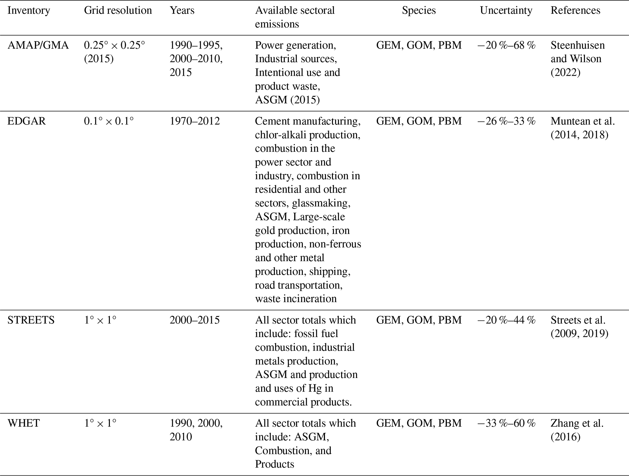
Figure 1 shows the latitudinal profiles of the annual anthropogenic Hg emissions (Mg yr⁻¹) and the spatial distribution of the TGM emissions range from the different inventories. Figure 2 presents the differences in emissions (Mg yr⁻¹) among the four different inventories by species and continent (in approximation using box masks). The percentage of emissions located in the Northern Hemisphere varies from 77.6 % to 88.5 % for the different inventories. There are multiple regions in Northern Canada, Alaska, the Sahel, northern Russia, and Australia where some inventories document zero emissions, and others report emissions. A comparison of inventories reveals large differences in Asia in terms of GOM and PBM emissions. Differences in GEM emissions are also pronounced in Asia, South America, and Africa. The overall chemical composition ratio GEM : (GOM + PBM) ranges between 1.83 and 4.57 for the different inventories.

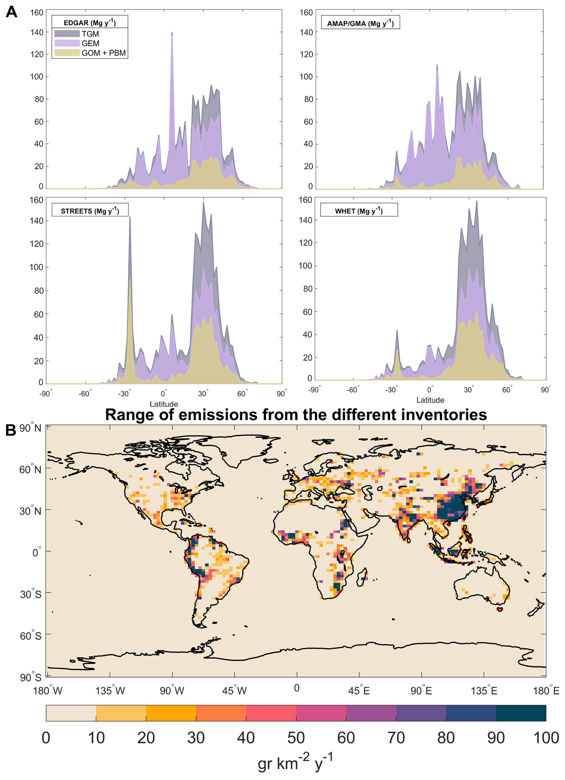
Figure 1 Panel (a) shows the latitudinal profile of annual Hg anthropogenic emissions (Mg yr⁻¹) and panel (b) the spatial distribution of the range of TGM emission from the different inventories and global emission estimates (g km⁻² yr⁻¹). The inventories correspond to different representative years: EDGAR (2012), AMAP/GMA (2015), STREETS (2013–2015), and WHET (2010).

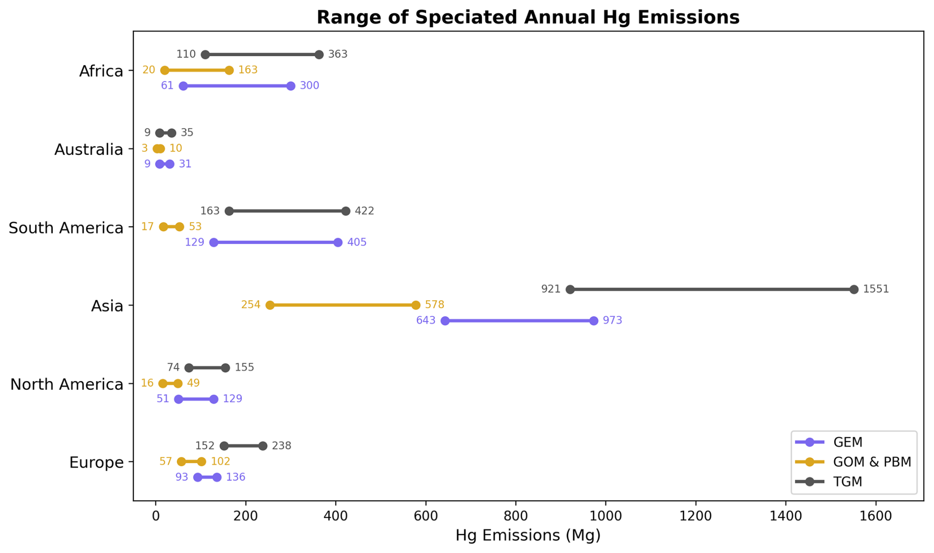
Figure 2 Range of speciated annual Hg emissions (in Mg) by continent, based on estimates from four different inventories. The inventories correspond to the following representative years: EDGAR (2012), AMAP/GMA (2015), STREETS (2013–2015), and WHET (2010).

2.2 Model and simulations

We used the GEOS-Chem model (v 12.8.01) (https://geoschem.github.io/, last access: 22 April 2024) for the Hg simulation (Horowitz et al., 2017) to estimate the effect of different uncertainties in modeling results at a horizontal resolution of 2° latitude by 2.5° longitude and 47 vertical levels. GEOS-Chem is driven by the assimilated meteorological MERRA-2 dataset and is parallelized using OpenMP. The simulations included three Hg tracers: GEM, GOM, and PBM. Both primary emissions and secondary re-emissions from soil and snow are included (Selin et al., 2008). The snow re-emissions are tied to solar radiation, and the re-emission rate used is based on the study of Durnford and Dastoor (2011). Legacy Hg reemissions from the ocean were archived from the MITgcm model (Horowitz et al., 2017), and monthly Br fields were taken from full-chemistry GEOS-Chem simulations (Schmidt et al., 2016), respectively. Surface–atmosphere Hg exchange processes, including soil, snow, and ocean re-emissions, are included in GEOS-Chem but are prescribed independently of the anthropogenic emission inventory used in each simulation. As a result, differences among anthropogenic emission inventories do not propagate into inventory-specific legacy re-emissions. This modeling choice allows isolation of the atmospheric uncertainty attributable to inventories of direct anthropogenic emissions. The atmospheric GEM oxidation mechanism considers gas-phase Br as the primary oxidant in the troposphere and stratosphere, and second-stage oxidation of HgBr by a number of radical oxidants (Horowitz et al., 2017). For half of the simulations, we used an alternative GEM oxidation mechanism (Selin et al., 2008) where the predominant oxidants are OH and O₃. More advanced chemical mechanisms have since been developed which incorporate the oxidation of Hg⁰ of both OH and Br, followed by oxidation by O₃ in a second-step (Castro et al., 2022; Shah et al., 2021; Saiz-Lopez et al., 2020, 2025). Nevertheless, by conducting two sets of simulations with radically different chemistry schemes (Br vs. OH/O₃), we can identify which regions of the atmosphere are most affected by chemical uncertainties. The model also calculates spatial fields of wet deposition of GOM and PBM consisting of scavenging in wet convective updrafts and rainout and washout in large-scale precipitation (Liu et al., 2001) and dry deposition of all three species. GEOS-Chem uses a formulation consistent with a resistance-based GEM dry deposition (Wesely, 1989).

Table 2 Simulations performed with the GEOS-Chem model (v 12.08.01).

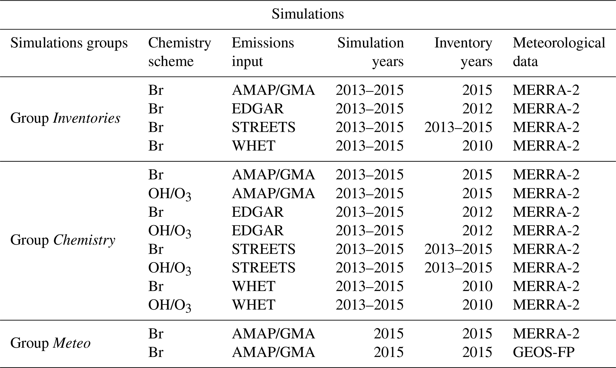
Our model experiments (Table 2) are designed in three groups to compare the magnitudes of model uncertainties driven by anthropogenic emissions, chemistry, and meteorological data. Each group was constructed by varying one input while holding others constant to isolate its influence on model output. To assess anthropogenic emissions uncertainty, we conducted the Inventories simulations, consisting of four simulations with the Br oxidation scheme, each utilizing a different inventory of anthropogenic emissions. To evaluate chemistry uncertainty, the Chemistry simulations comprise eight simulations. This group includes four simulations using the Br oxidation scheme, each with a different inventory of anthropogenic emissions, as well as four simulations utilizing the OH/O₃ oxidation scheme, which are also based on different inventories of anthropogenic emissions. These simulations aim to highlight potential differences resulting from the selection of chemical mechanisms, clarifying their contribution to modeled atmospheric processes. The output variables from each set of simulations were averaged to obtain their means, which were then compared to represent the chemistry uncertainty. A 2-year spin-up period was used for the Inventories and Chemistry simulations and the results from the third, fourth, and fifth years, 2013, 2014, and 2015, were used for the analysis as a multi-annual mean (2013-2015). For the Meteo simulations group, we ran the model twice for the year 2015 using the Br oxidation scheme and the AMAP/GMA emission inventory, each time based on a different meteorological dataset: MERRA-2 and GEOS-FP.

2.3 Measurements

GEM observations are obtained from the compilations of Travnikov et al. (2017) (courtesy of Hélène Angot) and AMAP/UNEP (AMAP/UNEP, 2019). The wet deposition flux observations are compiled by Travnikov et al. (2017) (courtesy of Hélène Angot), Sprovieri et al. (2017), AMAP/UNEP (AMAP/UNEP, 2019) and Fu et al. (2016). In this study, only observations collected between 2013 and 2015 are included.

2.4 SNR as a measure for extracting a model's uncertainty effect size under intra-annual variability

SNR compares the level of a signal of interest with the level of background noise (Welvaert and Rosseel, 2013). There is a substantial body of research that has used the SNR measure in atmospheric sciences (Acosta Navarro and Toreti, 2023; Doi et al., 2022; Yu et al., 2020; Hamilton and Hart, 2023; Hasselmann, 1979; Falkena et al., 2022). In our study, the SNR is used to identify regions where the model-observation studies are suitable for the evaluation of anthropogenic emissions uncertainty. In this case, the signal is defined as the range (maximum minus minimum) of the model output variable across all simulations within a group (e.g., Inventories, Chemistry, or Meteo). The noise is quantified by first calculating the temporal standard deviation of the model output for each individual simulation, and then averaging those standard deviations across all simulations in the group. This average represents the typical intra-annual variability used in the denominator of the SNR. A high SNR indicates a large signal (high propagated uncertainty to modeling results) compared to the noise (relatively small intra-annual variability). We apply SNR to modeled atmospheric Hg concentrations and wet deposition output to extract the signal due to anthropogenic emissions and other model uncertainties in the presence of intra-annual variability. We use the SNR as defined by the following equation:

$$\begin{array}{}\text{(1)}& \begin{array}{rl}\mathrm{SNR}& ={\displaystyle \frac{\mathrm{range}\mathrm{across}\mathrm{simulations}\mathrm{in}\mathrm{a}\mathrm{group}}{\mathrm{average}\mathrm{of}\mathrm{temporal}\mathrm{SDs}\mathrm{within}\mathrm{each}\mathrm{simulation}}}\\ & ={\displaystyle \frac{\max \left(x_i\right)-\min \left(x_i\right)}{\frac{\mathrm{1}}{n}\sum _{i=\mathrm{1}}^n{\mathit{\sigma }}_t\left(x_i\right)}}\end{array}\end{array}$$

where x_i is the output variable from simulation i, σ_t(x_i) is the temporal standard deviation for that simulation and n is the number of simulations in the group.

The range within each of the three simulation groups provides a representation of the uncertainties that arise from emissions, chemistry, and meteorology, respectively. We used the mean annual daily standard deviation (SD) as a direct measure of GEM, and weekly SD for wet deposition intra-annual variability. We used a weekly time frame for wet deposition because observation samples were collected on a weekly basis.

3 Results

3.1 SNR of major Hg modeling uncertainties

3.1.1 Stations' locations

We analyzed GEM data from 34 monitoring stations (Figs. 3, A1 and A5) aggregated in 6 wider regions and compared them with the variability in modeling results for the three different simulation groups (Inventories, Chemistry, and Meteo). The variability in the model output resulting from the emission input set is larger in four of the six regions (Asia, the United States, Europe, and the Arctic Circle) compared to the variability caused by chemistry or meteorology input sets. The effect of the meteorological data choice does not lead to considerable differences in the modeled GEM in any region.

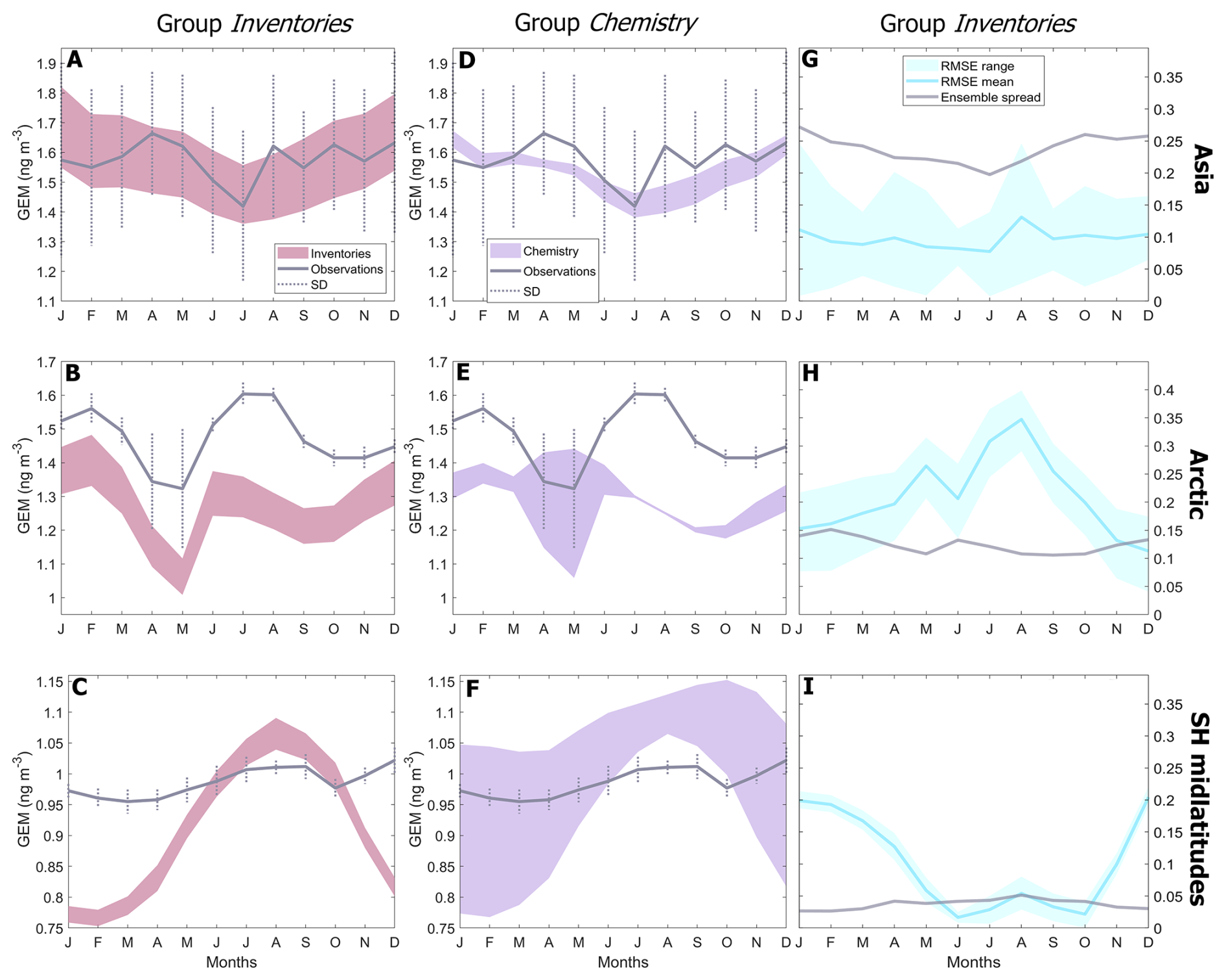
Figure 3 Seasonal variation of GEM (monthly averages and their SD among stations) for stations located in the Arctic, Asia and Southern Hemisphere mid-latitudes. The range of the simulated GEM is depicted in pink (a–c) and purple (d–f), respectively for the Inventories simulations group and Chemistry, respectively. The third column (g–i) shows the calculated RMSE range and mean, and the group range.

In Asia (Fig. 3a, d and g), the impact of the Hg oxidation pathway on modeled GEM is minimal, while the Inventories simulations group shows a range of up to ≈0.3 ng m⁻³. However, the range of the modeled GEM is not as pronounced as the variability in the observed GEM between different stations and days. Based on the inventories used in this study, Asia is the region with the largest emissions, contributing 51.5 %–68.9 % to global anthropogenic Hg emissions. The high level and spatial and temporal variability of observed GEM (Fig. 3a and g) indicate numerous continuous and episodic high-emitting sources.

In the Arctic, the range of simulated GEM in the Inventories simulations group is below the observations' range. A possible explanation is that, as the Arctic is primarily a receptor region, the long-range transport of Hg to the Arctic may be underestimated, or that sources contributing to Arctic Hg may be underestimated in current emission inventories. Several studies point to Asia, Europe, and North America as the main contributors to Hg concentrations in the Arctic (Dastoor et al., 2022; Durnford et al., 2010). As can be seen in Table 2, the annual GEM emission estimates differ by 330.5 Mg in Asia, 43.2 Mg in Europe, and 78 Mg in North America. In addition to the diversity in anthropogenic emissions inventories that lead to a wide range of RMSE for the Inventories simulations group, the RMSE reaches its highest point during the summer months. Although the model captures most of the seasonal effects, it is not capable of simulating the peak in GEM levels during the summer. A considerable amount of literature has been published on the maximum GEM concentration levels observed in summer, which are attributed to snow and sea ice melt and oceanic Hg reemissions (Angot et al., 2016a; Araujo et al., 2022; Huang et al., 2025; Yue et al., 2023).

In the Southern Hemisphere (SH midlatitudes, Antarctica and Australia regions), the chemistry scheme used to simulate GEM contributes more variability than the emissions inventory used (Fig. 3c and f). Recent findings indicate an atmospheric Hg lifetime of 3 to 6 months (Shah et al., 2021; Horowitz et al., 2017; Zhang and Zhang, 2022), which means that Hg emissions remain in the hemisphere of origin (Driscoll et al., 2013). A previous study of Hg source-receptor relationships using GEOS-Chem (Corbitt et al., 2011) found that extra-tropical sources have a particularly strong influence on regions within their own hemisphere. The anthropogenic emission inventories used in this study account for only 11.5 % to 22.4 % of global emissions located in the Southern Hemisphere, partially explaining their limited influence on model error analysis. The SH mid-latitude region includes Cape Point, Amsterdam Island, and Bariloche sites. Cape Point and Amsterdam Island are marine sites greatly influenced by the ocean (Angot et al., 2014; Schneider et al., 2023; Slemr et al., 2020). Given that 81 % of the Southern Hemisphere surface is ocean (Schneider et al., 2023), air–sea exchange processes are an extremely important component in the Hg cycle in this hemisphere (Bieser et al., 2020). The choice of Hg oxidation scheme leads to a significant impact in the modeled GEM in the Southern Hemisphere, as a result of the different distributions of Hg(0) oxidation and the chemical lifetime of tropospheric GEM.

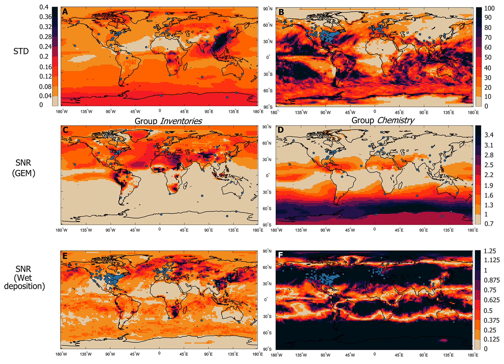
Figure 4 Spatial distribution of the daily monthly averaged SD of GEM (ng m⁻³) (a) and annual weekly-averaged SD of wet deposition (ng m⁻²) (b). SNR of GEM and wet deposition when using: different inventories (c, e) and different chemistry schemes (d, f).

3.1.2 Global

Model error signals can be obscured by noise in model-observation comparisons. To identify the extent of model error signals embedded in the background “noise” of natural variability, we examine the SNR. Figure 4a illustrates the global annual daily-averaged SD of simulated GEM for the group Inventories. The model estimated a markedly high intra-annual variability of GEM in areas characterized by exceptionally high emission levels, such as South and East Asia, which is also observed on a monthly basis through observations (Fig. 3g). A high intra-annual variability of GEM is found in Antarctica and generally in more southern latitudes as corroborated by the Fig. A1 and several publications (Angot et al., 2016a, b, c; Temme et al., 2003; Dommergue et al., 2013, 2010; Sprovieri et al., 2002). The global map in Fig. 4b displays the annual weekly-averaged SD of wet deposition. SD of wet deposition is high over the oceans and is also evident in some regions of eastern North America and South America.

The results obtained using the SNR analysis of the GEM model outputs for the Inventories and Chemistry simulations groups are illustrated in Fig. 4c and d. For the Group Meteo, the Fig. A4 shows SNR greater than 1 for GEM only over the equatorial western part of South America. The SNR patterns for simulation groups Inventories and Chemistry are largely anti-correlated, with values exceeding 1 in one group typically corresponding to lower values in the other. Annually averaged GEM measurements in the Northern Hemisphere provide an optimal and independent constraint for evaluating uncertainties in anthropogenic emission inventories, distinct from other uncertainty signals considered in this study. The US Atmospheric Mercury Network (AMNet), particularly the eastern zone, constitutes one of the most reliable monitoring systems for the Hg emission inventory assessment using GEM measurements. However, even though there are numerous stations located in areas with high SNR during winter months, the monitoring networks remain spatially limited, resulting in insufficient coverage of areas with high SNR, including Greenland, the Mediterranean Sea, Arctic Russia as well as regions in South America, and Africa. In contrast, relatively continuous GEM measurements in the mid- and high-latitude regions of the Southern Hemisphere are better suited to isolate and assess uncertainties in the chemical mechanisms, as these regions exhibit low SNR for anthropogenic emissions and pronounced impact of chemical scheme choices (Fig. 4d).

Figure 4e and f depict the results derived from the SNR analysis applied to the wet deposition model outputs for the Inventories and Chemistry simulations groups. Figure A4 presents the SNR for wet deposition in the Group Meteo, indicating a moderate signal strength in wet deposition in the Southern Hemisphere. The SNR measure illustrates that wet deposition measurements are less sensitive to the change in anthropogenic emissions within the Inventories simulations group (Fig. 4e), as compared to GEM measurements (Fig. 4c). Nonetheless, there exist specific regions where the SNR attains a value of 1, with some of these locations also coinciding with monitoring stations (East Asia). On the other hand, the SNR pattern of the ensemble Chemistry reveals strong signals throughout the globe except in the subtropical areas. Several studies have identified errors or gaps in the chemical mechanisms related to the atmospheric oxidation of GEM, which is a critical precursor to both wet and dry deposition processes (Wang et al., 2014; Skov et al., 2004). The SNR for wet deposition in the group Meteo indicates a wider moderate SNR in wet deposition throughout North America, Europe, and South Asia.

3.1.3 Seasonality

Figure 5 presents the SNR pattern over the globe for different seasons. While the SNR is consistent over seasons in some regions, in others, the SNR demonstrates seasonal variation, controlled by seasonal patterns such as meteorological conditions and atmospheric chemistry. The Mediterranean Sea, eastern US, and eastern Russia do not show significant seasonal changes in the SNR, making them ideal regions for observationally-based emission evaluation throughout the year. For the Arctic and northern Eurasia, the winter months have a higher SNR. Winter is the most promising period to evaluate emission uncertainties through GEM background concentrations in the Arctic, as it is not influenced by local chemical processes that could introduce sources of noise (e.g. AMDEs; Steffen et al., 2008; Skov et al., 2020). In the central and western US, the decrease in SNR in autumn is likely due to increased GEM anomalies caused by meteorological factors (Xu et al., 2022). In Europe and central Eurasia, the response of modeled GEM on emissions uncertainty is higher during the winter. However, the model results suggest low SD of GEM during the summer resulting in a high SNR (Fig. 5c).

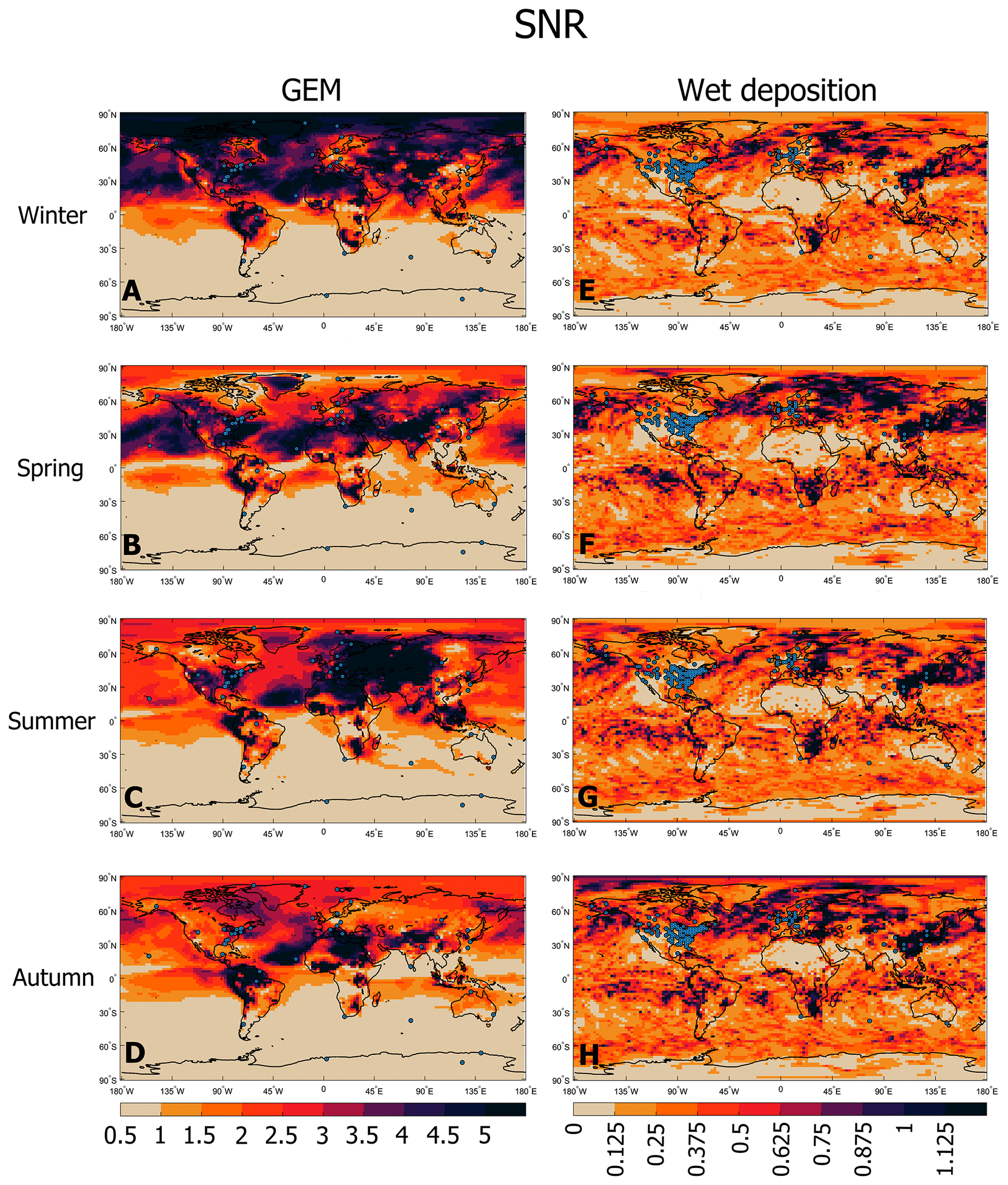
Figure 5 Seasonality of SNR of: GEM (a–d) and wet deposition (e–h) for the Group Inventories.

Even intra-annually, the signal of emissions uncertainties rarely exceeds the noise (Fig. 5e–h) in modeled wet deposition. In particular, Australia and South America have very low SNR values. The low signal and high variability of modeled wet deposition indicate that they hamper the evaluation of emissions uncertainties or even hide anthropogenic emissions effects on wet deposition. The exception is in northeast Asia, where the detection capability of emissions uncertainty on modeled wet deposition appears to be >1 throughout the year. In contrast to the SNR based on the modeled GEM, the SNR based on the wet deposition is greater than 1 in spring and autumn in the Arctic (Fig. 5f and h). The extended spatial spread of SNR greater than 1 in the Arctic during the autumn results from a low SD of wet deposition of Hg. This means that measuring wet deposition and assessing emissions in autumn could give insights into the northern hemispheric background Hg. In the springtime, in the Arctic and in Central North Russia, isolating the emissions uncertainty signal in spring is more efficient.

3.2 Discussion

CTMs are typically evaluated based on their performance in simulating atmospheric Hg concentrations and deposition. In contrast, this study focuses on assessing how modeling choices affect the robustness of CTMs when used to evaluate anthropogenic Hg emission inventories. As the bottom-up method for Hg emission estimation suffers from various uncertainties and the current anthropogenic Hg inventories differ by substantial amounts, independent constraints from observations could shed light on primary anthropogenic Hg emissions uncertainties. Our simulations generate insight into which sites could provide or not the most relevant constraints on primary anthropogenic Hg emissions.

This modeling experiment reveals that different regions of the world exhibit varying levels of sensitivity to model components, such as emissions and atmospheric chemistry. The large differences in anthropogenic emissions estimates for Asia dominate the variability in modeled GEM. However, when considering aggregated monitoring sites across Asia, the resulting discrepancy in modeled GEM may not always be easily constrained by model-observation comparisons using the current observation sites. The reason is that, in this case, the range of the model results falls within the range of GEM measurement variability (Fig. 3a), which partly reflects spatial aggregation of heterogeneous monitoring locations. The spatial SNR patterns shown in Fig. 4c highlight subregional differences. For example, central China and Central Asia exhibit relatively high SNR values, whereas eastern China shows lower SNR. While the largest absolute uncertainties in anthropogenic Hg emissions occur in Asia and South America, our analysis identifies regions where background observations are most effective at isolating emission signals from other sources of variability, which is a distinct but complementary objective.

Based on our modeling results, we show that current SH monitoring networks are not ideal to help evaluate anthropogenic emissions uncertainties, but they could be instrumental in addressing uncertainties related to chemical processes. Current observations in the SH are insufficient to evaluate anthropogenic emissions uncertainties due to distances from areas with positive SNR (apart from the Nieuw Nickerie and Manaus sites) and their limited spatial coverage (Fig. 4c). The majority of GEM observation sites in the SH are located in areas where chemistry uncertainty and intra-annual variability completely impede detection signals of anthropogenic emissions uncertainty. For instance, when analyzing the annual averaged results for the SH mid-latitudes and Antarctica, the response of the model across different emission inventories remains below 0.06 and 0.04 ng m⁻³ range of GEM, respectively. The low sensitivity to the different inventories in conjunction with up to 0.2 ng m⁻³ intra-annual variability of GEM leads to very low SNR across much of the Southern Hemisphere monitoring network. However, this result should not be interpreted solely as evidence of a true physical insensitivity of Southern Hemisphere Hg concentrations to anthropogenic emissions. The weak emissions SNR may also reflect limitations in currently available anthropogenic Hg emission inventories for the Southern Hemisphere, where emissions from ASGM and industrial sources are known to be poorly constrained (AMAP/UNEP, 2019). Future studies could address this point using new emissions inventories that have been published after these simulations were completed (Qiu et al., 2025; Muntean et al., 2024; Cui et al., 2025; MacFarlane et al., 2022). In this context, a low SNR may arise from an under-representation or misallocation of anthropogenic emissions in the input data. Improved bottom-up emission estimates and enhanced observational coverage in the Southern Hemisphere could therefore improve the ability of monitoring networks to constrain anthropogenic Hg emissions uncertainties.

The chemistry and meteorological data model settings and the intra-annual Hg variability have less impact on model-simulated Hg concentrations and wet deposition in Europe, the USA, and the Arctic. The model and the observations agree that the SD of GEM for the Arctic Circle (Fig. 3h), USA (Fig. A1i), and Europe (Fig. A1h) monitoring systems is low (smaller than 0.09 ng m⁻³) for any month of the year. Distinguishing emissions uncertainty signals over intra-annual variability of GEM in the sites of the Arctic Circle is feasible, as the former is more than twice as large as the latter. In winter, SNR exceeds the value of 5.5 in both Greenland sites. Similarly, sites that could help constrain the uncertainties of anthropogenic emissions are those in South Europe and the East US. While the SNR analysis identifies regions such as the Arctic and specifically Arctic Russia, Greenland, as theoretically optimal for isolating anthropogenic Hg emission signals – particularly during winter – these findings should be interpreted in the context of substantial real-world constraints. Harsh environmental conditions, including extreme cold, prolonged darkness, snow and ice cover, and limited accessibility, pose significant operational challenges for sustained monitoring in the Arctic. In addition, strengthening monitoring coverage in remote areas such as Greenland and Arctic Russia faces logistical, infrastructural, and geopolitical constraints.

Studies of Hg emissions and atmospheric processes that are performed using a single model present advantages but also limitations. One advantage of employing one model is that it allows a controlled and consistent framework to systematically evaluate specific uncertainties, such as those arising from emission inventories, chemical mechanisms, or meteorological datasets. With this approach, it is possible to focus on specific sources of modeling uncertainty and derive more accurate conclusions within a specific, invariant model architecture. Additionally, an experiment with a single model often reduces computational costs and complexity, facilitating performing a group of simulations within a consistent modeling environment. Despite its benefits, this method entails certain limitations. A single model inherently reflects the biases and limitations of its design, such as its specific treatment of Hg chemistry or resolution constraints. Such biases may result in overconfidence in findings, which might not apply to other models. On the other hand, multi-model studies enable exploration of the diversity of outcomes, which commonly improve the robustness of the analysis of uncertainty and confidence in predictions. To address this issue, our study incorporated two fundamentally different chemistry schemes, representing distinct oxidation pathways (Br and OH/O₃-based chemistry), within the same modeling framework. Using these different chemical schemes allowed us to cover a broad range of chemical uncertainties and reduce the potential for bias linked to dependence on a single chemical mechanism. Future studies could conduct similar analysis using other global mercury models (Dastoor et al., 2025), as well as updated Hg chemistry schemes (Saiz-Lopez et al., 2025; Shah et al., 2021).

One limitation of the present analysis is that inventory-dependent re-emissions are not represented. The modeled response to anthropogenic emission differences likely underestimates the full influence of emissions on atmospheric Hg. Such an approach is beyond the scope of the present work and would complicate attribution of modeled atmospheric differences to specific sources of uncertainty. Therefore, our results should be interpreted as a lower-bound estimate of the relative importance of anthropogenic emission uncertainties compared to chemistry and meteorology. Additionally, the Meteo simulations are intended to assess sensitivity to commonly used assimilated meteorological datasets within the GEOS-Chem framework rather than to represent the full range of meteorological model uncertainty.

To effectively reduce anthropogenic Hg emission estimate uncertainties and support global Hg policy goals, the design of Hg monitoring networks could better target regions with high SNR of anthropogenic emissions uncertainties and minimal overlapping signals from multiple other sources (e.g., chemistry, and meteorology). The eastern US, Greenland, and Arctic Russia (Fig. 4c), are ideal locations for year-round monitoring to evaluate the potential uncertainties of anthropogenic Hg emission inventories. Such regions with high SNR can effectively minimize background noise and isolate clear signals of anthropogenic Hg emissions. For example, the whole Arctic's high SNR during winter months (Fig. 5) makes it an excellent location for studying Northern Hemisphere background Hg concentrations, independent of other chemical or meteorological errors in modeling results (Figs. 4d and A4). Additionally, regions like Eurasia, northern Canada, and central North America show high SNR during specific seasons (Fig. 5), making them key areas for detecting emissions uncertainty, particularly in seasons when Hg transformation or deposition processes are more stable.

Key regions for intensive monitoring include high-emission regions such as Asia, South America, and Africa, where ASGM and industrial activities prevail. With China and India producing high industrial, and coal combustion Hg emissions, Asia is the biggest emitter (AMAP/UNEP, 2019). Identifying and quantifying such sources of high emission remains a major challenge, and an enhanced strategy and dense monitoring are needed to reduce associated uncertainties. Monitoring stations could be densely distributed in these regions to capture the full range of emissions and their shifts in space and time (Fig. 2a, d and g) and better estimate anthropogenic Hg emissions. The main sources of emissions in South America and Africa are ASGM, fuel combustion, and industrial activities (AMAP/UNEP, 2019), and targeted monitoring strategies are necessary to address the significant uncertainties in Hg emissions from these activities. Large portions of the globe remain undersampled, including parts of Africa, South America, and Asia. Measurements in these areas are important for improving the understanding of Hg sources. Expanding the global monitoring network would complement observations in high-emission and high-SNR regions and strengthen model–observation comparisons used to evaluate Hg emissions and atmospheric processes. In addition, tailored wet deposition monitoring in regions like Asia and South Africa, where emission estimates vary widely, is essential to constraining emissions, as the high SNR suggests strong potential to constrain model uncertainties (Fig. 3e). Although enhanced wet deposition monitoring in regions such as South Africa may be informative from a modeling perspective, such recommendations must be considered alongside regional climatology. Much of southern Africa is characterized by arid or semi-arid conditions and recurrent droughts, limiting the feasibility and interpretability of continuous wet deposition measurements.

In addition to high-emission zones, remote receptor regions, such as the Arctic, are instrumental in capturing long-range Hg transport and deposition. The Arctic, as a receptor region, is of considerable importance in understanding global Hg transport, especially from major emitting regions such as Asia, Europe, and North America. However, current modeling underestimates GEM in this region (Fig. 3b, e and h), making it imperative to enhance monitoring efforts in Greenland and Arctic Russia (Fig. 4c). Monitoring in these remote locations will provide baseline data to shed light on the causes of model-observation discrepancies as well as anthropogenic emission uncertainties.

Observations should be consistently used in model–observation comparison studies with CTMs such as GEOS-Chem to ensure that the monitoring network provides actionable insights for policy-makers and the Minamata Convention on Mercury. In this way, refinement of Hg emission estimates would be possible, especially in regions where significant discrepancies exist between observed and modeled data. The benefits of using inverse modeling techniques (Song et al., 2015) are also important in constraining emission inventories based on observations. Inverse modeling refines Hg emission estimates by adjusting model inputs to better match observations like GEM or wet deposition. Using models such as GEOS-Chem, emissions are iteratively optimized to minimize differences between simulations and observations. This top-down approach is especially useful to identify and correct inventory biases. Therefore, strengthening the monitoring network would not only enhance our understanding of the Hg global distribution and deposition but also provide critical data to guide future policy interventions aimed at reducing global Hg emissions.

For the Hg modeling community, this study points to the importance of addressing both emissions and other model uncertainties simultaneously rather than in isolation. The complex interactions between emission inputs, chemical processes, and meteorological data require models to be tested holistically. As demonstrated in this work, emission uncertainties could mask the impacts of other model errors regarding Hg wet deposition (Central America, Fig. 4c and d), and vice versa. Therefore, to minimize overall uncertainty, model developers and users should not only improve the accuracy of emission input data but also refine the representation of key atmospheric processes within models, such as Hg oxidation and deposition mechanisms. This dual approach is essential because, as shown in this study, uncertainties in emissions and chemistry can interact and amplify total model uncertainty in complex ways.

4 Conclusion

This study offers a better understanding of the role of anthropogenic Hg emission uncertainties in the performance of global Hg models, underscoring the need for more precise emission inventories and monitoring strategies for their evaluation. We have demonstrated that differences among emission inventories, particularly in high-emission regions like Asia, can introduce significant differences in modeled GEM concentrations, especially in the NH, with regional discrepancies across modeling results reaching up to 0.47 ng m⁻³. Our findings indicate that the chemistry scheme is the prevailing factor influencing Hg concentrations in the Southern Hemisphere, exerting a greater impact than anthropogenic emissions input. These findings demonstrate that intercomparison studies should include region-specific evaluations, recognizing that model accuracy may vary geographically based on different driving factors, rather than focusing only on global model performance. This important effect of anthropogenic emission uncertainties in modeling results leads to a range of RMSE scores in model-observations comparisons that could provide incomplete information about the NH distribution of Hg. Our findings identify high SNR regions, such as Greenland and the eastern US, Arctic Russia, and parts of Asia and South America, that can provide reliable observational data to help constrain anthropogenic emission uncertainties and improve model accuracy. The Hg modeling community can improve the reliability of simulations by incorporating more accurate and region-specific anthropogenic Hg emission inventories into models. Trends in atmospheric Hg concentrations, Hg deposition fluxes, changes in national emissions reports provided by Parties, and insights derived from modeling approaches are primary indicators for the effectiveness evaluation under the Minamata Convention (United Nations Environment Programme, 2023). Accurate and consistent emission inventories are essential components in mercury studies, acting as a basis for explaining observed atmospheric trends, verifying reported emissions reductions, and supporting modeling efforts with greater accuracy. The analysis indicates that current uncertainties in emission inventories, particularly in Asia, South America, and Africa, present a significant barrier to reliably assessing progress under the Convention's effectiveness evaluation framework. On a wider level, the results of this study are encouraging collaborative efforts for the refinement of emission inventories and improvement of the accuracy of global Hg models to support policy interventions aimed at mitigating Hg pollution.

Appendix A

Table A1 Bounding coordinates that were used to calculate the anthropogenic Hg emissions by continent.

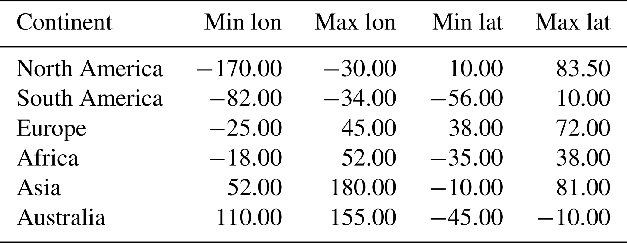
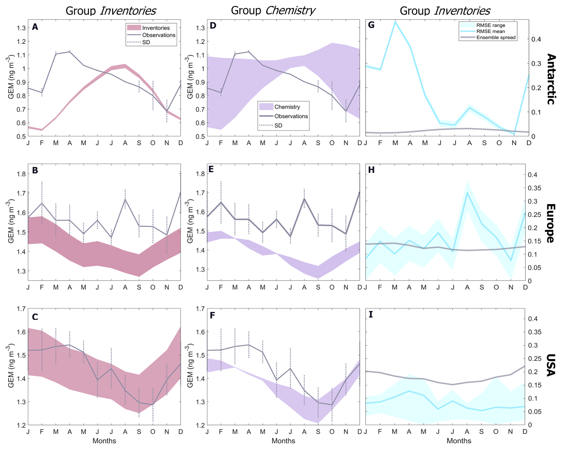
Figure A1 Seasonal variation of GEM (monthly averages and their SD among stations) for stations located in the Antarctic, Europe, and the USA. The range of the simulated GEM is depicted in pink (a–c) and purple (d–f), respectively for the Inventories simulations group and Chemistry respectively. The third column (g–i) shows the calculated RMSE range and mean and the group range.

Figure A2 Range of the daily annual mean Hg concentrations for the group of simulations Inventories.

Figure A3 Range of the weekly Hg wet deposition for the group of simulations Inventories.

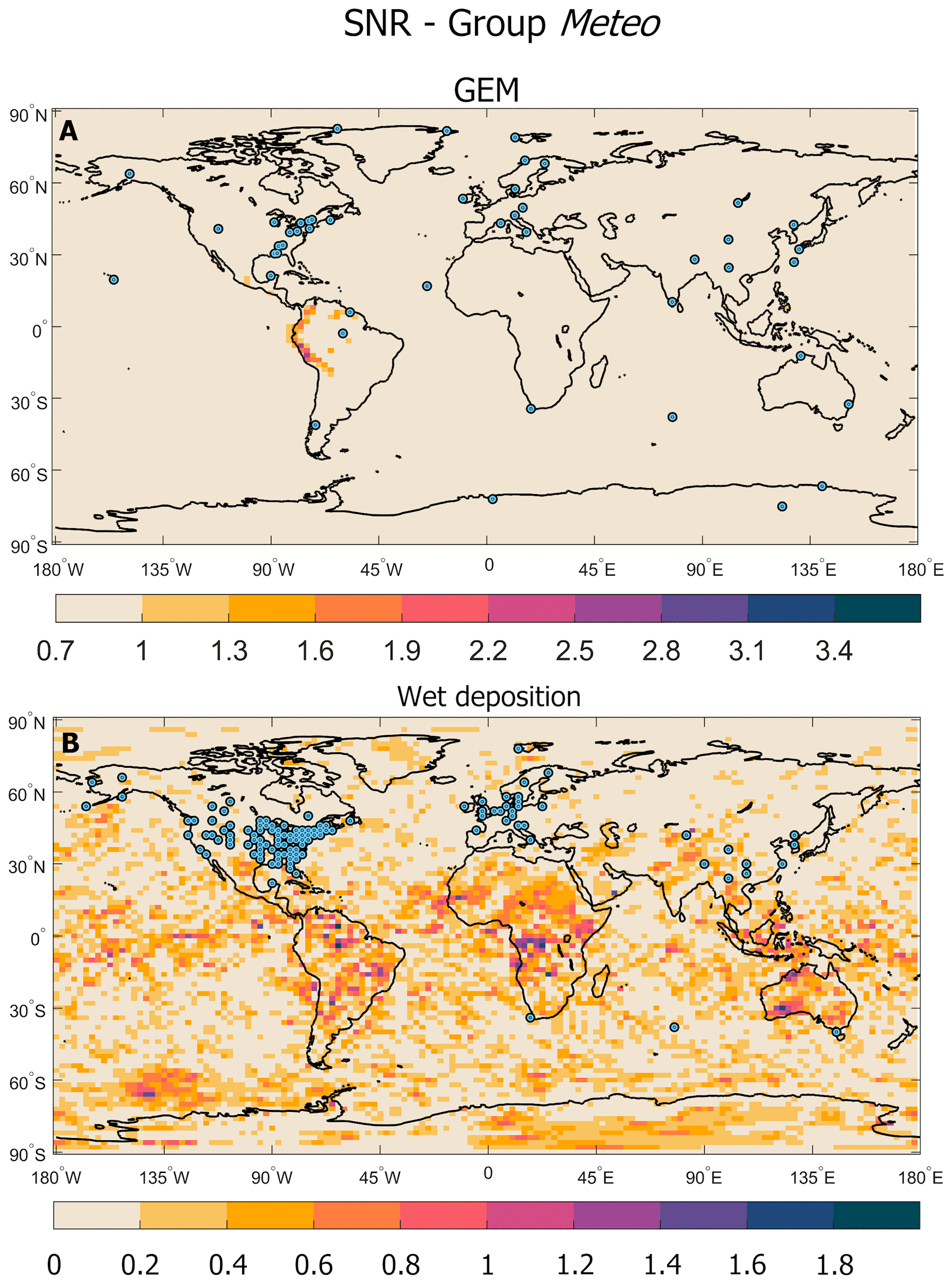
Figure A4 SNR of (a) GEM and (b) wet deposition for the group of simulations Meteo.

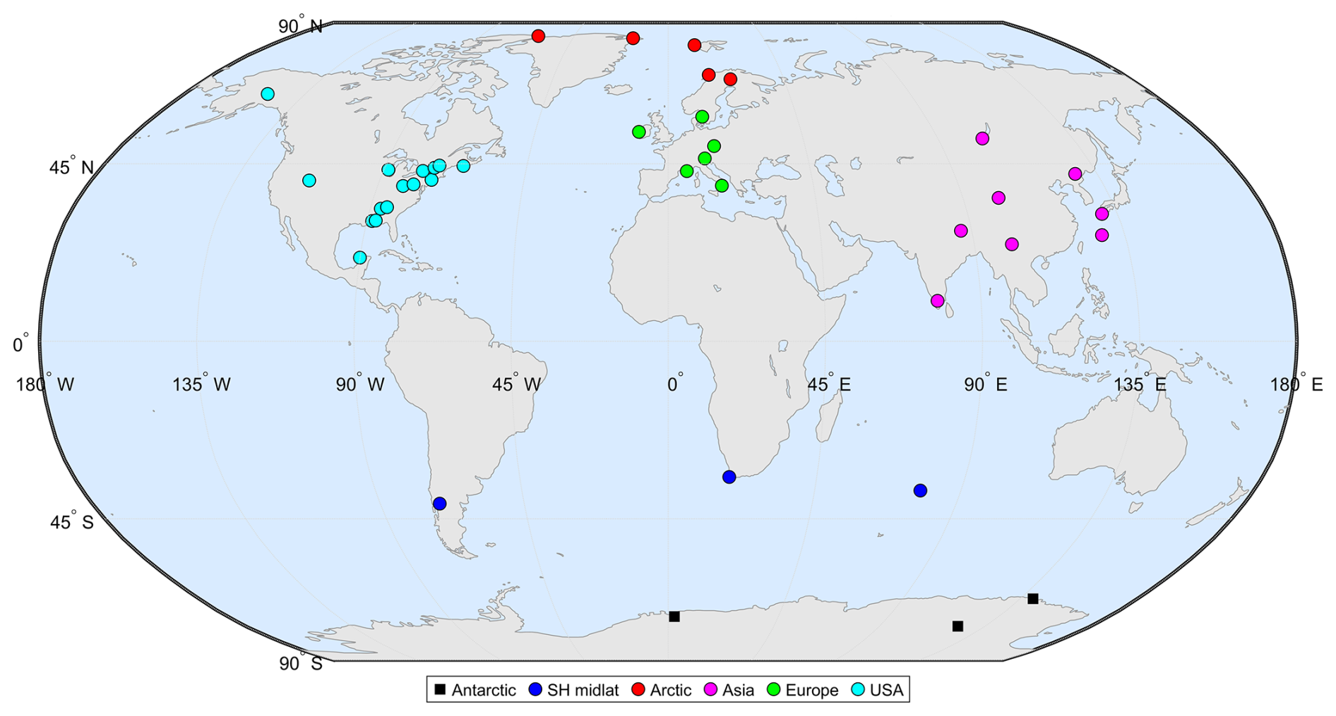
Figure A5 Geographic distribution of categorized GEM monitoring stations used in this study for analysis. Stations are grouped into six regions: Antarctic, Southern Hemisphere midlatitudes, Arctic, Asia, Europe, and USA.