the Creative Commons Attribution 4.0 License.
the Creative Commons Attribution 4.0 License.
 | 15 Apr 2026
14C-based separation of fossil and non-fossil CO2 fluxes in cities using relaxed eddy accumulation: results from tall-tower measurements in Zurich, Paris, and Munich
Ann-Kristin Kunz
Samuel Hammer
Patrick Aigner
Laura Bignotti
Lars Borchardt
Julian Della Coletta
Lukas Emmenegger
Markus Eritt
Xochilt Gutiérrez
Josh Hashemi
Rainer Hilland
Christopher Holst
Armin Jordan
Natascha Kljun
Richard Kneißl
Changxing Lan
Virgile Legendre
Ingeborg Levin
Benjamin Loubet
Matthias Mauder
Betty Molinier
Susanne Preunkert
Michel Ramonet
Stavros Stagakis
Andreas Christen
Relaxed eddy accumulation (REA) measurements for 14CO2 enable the estimation of fossil fuel (ff) CO2 fluxes in urban areas. This work is based on 252 REA ffCO2 flux measurements conducted on tall towers in the cities of Zurich, Paris, and Munich. The ffCO2 fluxes were compared to net eddy covariance CO2 fluxes to quantify the role of non-fossil (nf) CO2 fluxes. While the measurements in Zurich and Paris were limited by small signal-to-noise ratios, improvements in the REA setup, the 14CO2 measurement precision, the sampling strategy, and the source strength increased the significance of the results in Munich. Large nfCO2 fluxes observed in Munich from the direction of a brewery demonstrate the efficacy of the partitioning approach and illustrate the complexity of urban atmospheric measurement data. Excluding these measurements potentially influenced by large anthropogenic nfCO2 fluxes, the error-weighted average ffCO2 CO2 flux ratio in Munich was approximately 47 % in summer and 76 % in winter, with the majority of measurements taken between 07:00 and 19:00 local time. Regional excess concentrations had much lower ffCO2 contributions (<63 % in winter and <28 % in summer, in all three cities), demonstrating fundamental differences between local and regional CO2 fluxes. The combination of 14CO2 observations and the REA method is a sophisticated approach that challenges the limits of current analytical capabilities, while providing unique opportunities for quantifying ffCO2 and nfCO2 fluxes.
- Article
(8736 KB) - Full-text XML
- BibTeX
- EndNote


Cities are hotspots for fossil fuel (ff) CO2 emissions and are at the heart of emission reduction efforts. To guide and monitor the pathways of cities towards climate neutrality, measuring and modeling urban ffCO2 emissions is essential. While total CO2 fluxes can be measured using the eddy covariance (EC) method, direct observations of fossil or non-fossil CO2 are lacking. However, a separation of the two components is important because, in addition to ffCO2 emissions, biospheric and human respiration fluxes play a substantial role in the urban carbon budget (e.g. Kellett et al., 2013; Miller et al., 2020; Wu et al., 2022; Stagakis et al., 2025). Several studies have attempted to separate ffCO2 and nfCO2 fluxes. Wu et al. (2022) combined CO2 fluxes from EC measurements and CO fluxes from flux-gradient measurements to estimate turbulent ffCO2 fluxes on a tower in Indianapolis 30 m above ground level, assuming a constant CO ffCO2 flux ratio. The latter was determined from CO and 14CO2 concentration measurements of flask samples collected weekly at the measurement site and an upwind background station, following Levin et al. (2003). Hilland et al. (2025) proposed a linear mixing model to separate biospheric, road traffic, and stationary combustion CO2 fluxes using simultaneous tall-tower EC measurements of CO2 and co-emitted species (CO and NOx), as well as sector-specific, constant flux ratios determined from a bottom-up emission inventory. Other studies used 14CO2 observations to separate fossil and non-fossil CO2 enhancements relative to a background concentration (e.g., Levin et al., 2003; Turnbull et al., 2015; Miller et al., 2020). In this case, surface emissions can be estimated using atmospheric transport models or the Radon-Tracer-Method, for example (Levin et al., 2003; Maier et al., 2024b). The source area thereby depends on the choice of the background station and includes a large region beyond the city boundaries if a tropospheric or continental clean air background site is used (Turnbull et al., 2015). To our knowledge, all previous studies estimating urban ffCO2 emissions relied on bottom-up information, inverse modeling results, or assumed constant proxy ffCO2 ratios, despite the fact that ratios such as CO ffCO2 vary significantly with fuel carbon content and combustion conditions (Turnbull et al., 2015; Maier et al., 2024a).
We overcome these limitations using 14CO2 relaxed eddy accumulation (REA) measurements, as first described in Kunz et al. (2025a). On a tall tower over the city, air is conditionally collected during one hour in two separate reservoirs (an updraft and a downdraft reservoir) using fast-switching sampling valves. The valves respond to a 20 Hz vertical wind signal from a 3D ultrasonic anemometer. Transfer of the collected air to portable glass flasks enables 14CO2 and CO2 measurements in a subsequent laboratory analysis, and thus the estimation of ffCO2 concentration differences between updraft and downdraft samples. Combined with net CO2 fluxes measured by open-path or closed-path EC, this novel approach enables the estimation of ffCO2 fluxes for the respective, hour-long sampling periods.
In Kunz et al. (2025a), the REA flask sampling system was described and its performance was analyzed in detail. It was shown to meet high technical requirements, e.g., fast and accurate switching between updraft and downdraft sampling, while maintaining a constant flow rate in sampling and non-sampling modes. For the estimation of ffCO2 fluxes, uncertainties due to the sampling procedure were negligible compared to the analytical 14CO2 uncertainty in the lab. Analysis of concentration differences between updraft and downdraft flask samples collected during a pilot application at a tall tower in Zurich, Switzerland, showed that separation of fossil and non-fossil components of the CO2 concentration differences is feasible, but often limited by a low signal-to-noise ratio of the 14CO2 difference. Since then, the REA system has been further improved and operated on two tall towers in Paris, France, and Munich, Germany, for another 9 months each.
This paper presents and analyzes the ffCO2 fluxes obtained from a total of 252 discrete hour-long 14CO2 REA measurements conducted on three tall EC towers in Zurich, Paris, and Munich. After a brief presentation of the methods (Sect. 2) and the measurement campaigns (Sect. 3), the following questions are addressed:
- Q1.
To what extent do 14CO2 REA measurements enable the separation of local fossil and non-fossil CO2 fluxes in an urban area? (Sect. 4.1, 4.2, 4.3)
- Q2.
- Q3.
How does the composition of surface fluxes in the vicinity of the tall tower compare to the composition of regional CO2 concentration enhancements? (Sect. 4.5)
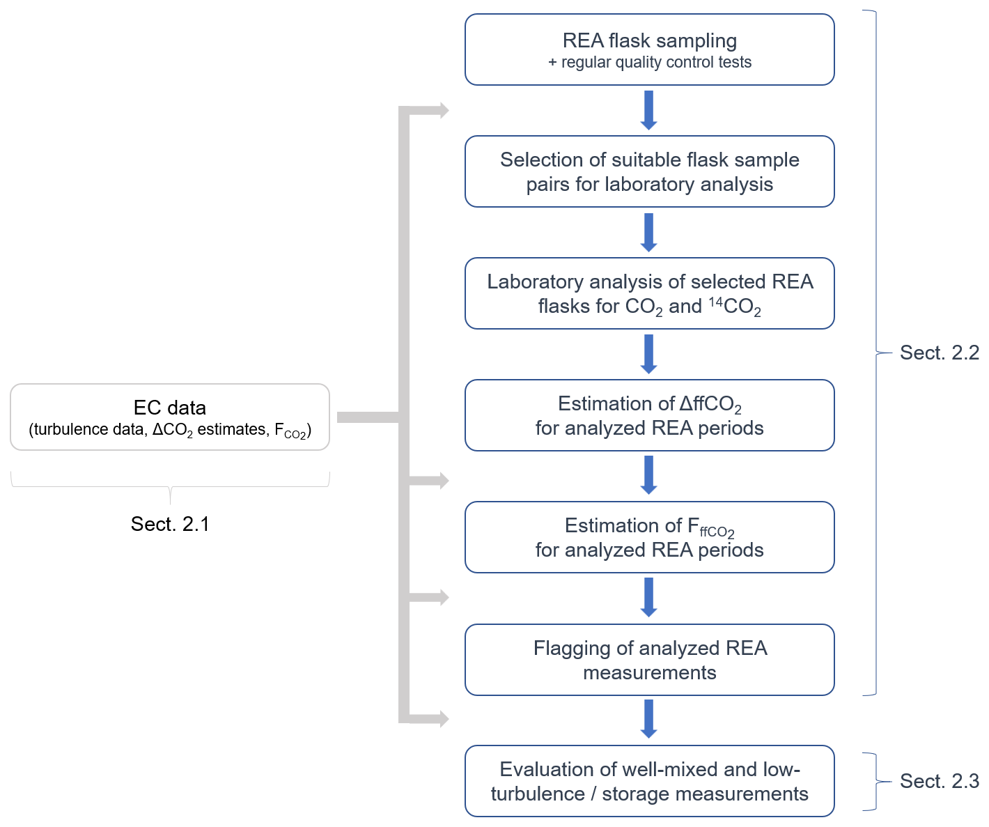
Figure 1Overview of the REA measurement and analysis procedure. ΔCO2 and ΔffCO2 denote the concentration differences between updraft and downdraft REA flask samples. is the 14C-based ffCO2 flux. “Well-mixed” and “low-turbulence/storage” measurements are two categories, in which the analyzed REA measurements considered in this study were divided based on several flagging criteria.
This study analyzes the contributions of fossil and non-fossil sinks and sources to net CO2 fluxes measured successively on three different urban tall towers for about nine months each. While the net CO2 fluxes were measured continuously by the well-established EC method (e.g., Aubinet et al., 2012b), the partitioning of individual, hour-long measurements is based on REA measurements for 14CO2 (Kunz et al., 2025a). Figure 1 provides an overview of the individual steps involved in the REA measurements and analysis.
In addition to CO2, the flask samples were also analyzed for CO, CH4, N2O, SF6, H2, δ(O2 N2), δ18O, and δ13C. Moreover, the MGA7 provided continuous flux measurements of CO, CH4, NO, and NO2. These measurements are of great value, e.g., for a future analysis of proxy ffCO2 flux ratios needed for estimating continuous ffCO2 fluxes based on proxy measurements. However, a multi-species analysis is beyond the scope of this work.
2.1 Net CO2 fluxes from eddy covariance measurements
Net turbulent CO2 fluxes were computed from high-frequency CO2 measurements of a closed-path (MGA7, MIRO Analytical AG, Wallisellen, Switzerland) and an open-path gas analyzer with a co-located 3D sonic anemometer (IRGASON, Campbell Scientific, Inc., Logan, UT, USA). To remove erroneous spikes caused by instrument malfunction or obstructions in the path of the IRGASON gas analyzer (e.g., animals, dirt, rain, snow), the 20 Hz CO2, H2O, and vertical wind measurements of the IRGASON were despiked using a modification of the Median Absolute Deviation (MAD) method described by Mauder et al. (2013). To this end, measurements where the median absolute deviation was outside the upper and lower limits defined by Mauder et al. (2013) were removed; however, observations in which three or more consecutive outliers occurred were kept. The latter was necessary to retain peaks in concentrations caused by the intermittent nature of emission signals in the urban environment, which flask measurements have exemplarily proven to be real. The 10 Hz measurements of the MGA7 were upsampled to 20 Hz using a nearest-neighbor approach with a search window of 50 ms. The upsampled MGA7 data was then synchronized with the IRGASON data directly based on the high-frequency CO2 time series of the two instruments by finding the time lag of maximum correlation, as in Hilland et al. (2025). Erroneous time lags for periods with poor correlation between the CO2 time series (correlation coefficient <0.5), e.g., due to low IRGASON signal strength during a rain event, were linearly interpolated. The median time lag was 4.15 s in Zurich, 10.45 s in Paris, and 37.30 s in Munich. See Appendix D for details. The fluxes were then computed using the software EddyPro (Version 7.0.9, Licor Inc., Lincoln, NE, USA) with a 30 min averaging period, coordinate rotation via double rotation (Wilczak et al., 2001), time lag compensation through covariance maximization, and detrending via block average (Rebmann et al., 2012). High-pass filtering effects were corrected according to Moncrieff et al. (2004). For low-pass filtering effects, the correction by Moncrieff et al. (1997) was used for the IRGASON and the correction by Fratini et al. (2012) for the MGA7. Random errors of the turbulent flux estimates were calculated after Finkelstein and Sims (2001), and storage fluxes were estimated from concentrations and based on a single-point profile. Quality control flags of 0 (high quality), 1 (intermediate quality) or 2 (poor quality) were assigned to all flux estimates according to Mauder and Foken (2004), checking the assumptions of stationarity and well-developed turbulence. In addition, EddyPro outputs a large set of variables for each 30 min averaging period, including friction velocity u*, standard deviation of vertical wind velocity σw, and molar volume of ambient air va. Details on the EddyPro outputs in general and the processing of the IRGASON and MGA7 data in particular can be found in LI-COR (2021) and Hilland et al. (2025), respectively.
To estimate the mean CO2 fluxes during the specific, typically 60 min long REA flask sampling periods (Sect. 2.2), the 30 min EC fluxes were averaged, weighted by the fraction of the EC averaging period during which REA samples were collected. This means that each 60 min flux includes two to three 30 min fluxes (usually two, since most REA measurements were scheduled at the hour). The uncertainty of the 60 min flux was estimated by error propagation of the respective 30 min random uncertainty estimates. Any additional uncertainties arising from the measurement instrument or data processing options used were not considered. For quality control purposes, the maximum of the 30 min quality control flags, denoted QC in the following, was considered. Since the CO2 concentration measurements of the MGA7 showed a better agreement with the flask concentration differences measured between updraft and downdraft samples than the IRGASON measurements (Appendix E), and since the spectral-corrected fluxes of the two instruments showed very good agreement (Appendix D), the fluxes calculated from the MGA7 measurements were used when available, otherwise the fluxes calculated from the IRGASON were used. Information on which EC data set was used is provided for each REA measurement in Kunz et al. (2025b).
2.2 14C-based separation of fossil and non-fossil CO2 fluxes from relaxed eddy accumulation measurements
2.2.1 REA sampling and flux calculation
Fossil and non-fossil components of the CO2 flux measurements were separated by 14CO2 analysis of flask sample pairs conditionally collected using the REA flask sampling system described in detail in Kunz et al. (2025a). In summary, depending on the 20 Hz vertical wind measurements of the IRGASON's 3D ultrasonic anemometer (Sect. 2.1), air was collected through two co-located inlets with two fast-response valves into two separate reservoirs: one for updrafts, and one for downdrafts. After a sampling period of, e.g., 60 min, it was checked whether sufficient air has accumulated for a subsequent CO2 and 14CO2 analysis in the laboratory. If so, the accumulated air was transferred by an extended automated 24-port flask sampler into two 3 l glass flasks that could be analyzed in the laboratory (denoted as “successful” REA measurement in the following). Updraft and downdraft were thereby defined with respect to the mean vertical wind velocity , excluding a range of wind speeds centered around and scaled by the standard deviation of the vertical wind σw (scaling factor δ). This so-called deadband with half-width δ⋅σw was intended to increase the concentration difference and to reduce the number of valve switchings (Rinne et al., 2021). and σw were either calculated from the 30 min period before sampling start (pre-set deadband) or dynamically adjusted using a 15 min backward-looking averaging interval (dynamic deadband). The latter lead to a more equally distributed sampling of updrafts and downdrafts and was therefore better suited for changes in vertical wind statistics during the sampling period. The calculated fluxes are independent of the method used to compute the deadband, since this is taken into account in the β coefficient (see below) (Pattey et al., 1993). See Kunz et al. (2025a) for technical details on the REA sampling.
Due to the costs and logistics associated with flask sample analysis, only a limited number of successful REA measurements could be analyzed. The selected REA flask samples were analyzed for CO2 in the ICOS (Integrated Carbon Observation System) Flask and Calibration Laboratory in Jena, Germany, and for 14CO2 in the ICOS Central Radiocarbon Laboratory in Heidelberg, Germany. Based on these measurements, the ffCO2 differences between updraft and downdraft samples, in the following denoted as ΔffCO2, were estimated (Appendix A1, Kunz et al., 2025a). Under stationary and well-developed turbulence, the ffCO2 flux can then be estimated according to Eq. (1):
is the mean molar air density in mol m−3. The proportionality factor β depends on the joint probability distribution of variations of the vertical wind velocity and the gas concentration and on the deadband width (e.g., Pattey et al., 1993; Milne et al., 1999; Fotiadi et al., 2005b). Values <0.1 or >1 indicate non-ideal sampling conditions for REA measurements (Grönholm et al., 2008; Hensen et al., 2009; Osterwalder et al., 2016). Due to the availability of co-located EC measurements of net CO2 fluxes (Sect. 2.1), these measured CO2 fluxes were used to calculate β for each sampling period individually:
ΔCO2 is the CO2 concentration difference between updraft and downdraft flask samples measured in the laboratory and is the net CO2 flux measured by EC (Sect. 2.1). Assuming scalar similarity between CO2 and 14CO2, Eq. (2) can be inserted into Eq. (1):
Accordingly, the fossil contribution to the net CO2 flux equals the ΔffCO2 ΔCO2 ratio of the REA flask samples. The uncertainty of the ffCO2 flux was derived according to Gauss' law of error propagation from Eq. (3). For ΔCO2 and ΔffCO2, only the measurement uncertainties from the laboratory analysis were considered, as uncertainties due to the sampling process, e.g., a time lag between a change in vertical wind and a switching of the fast-response sampling valves, are negligible compared to the 14CO2 measurement uncertainty (Kunz et al., 2025a). The uncertainty of was estimated using the random uncertainty estimate from EddyPro (Sect. 2.1). Additional uncertainties, e.g., due differences between IRGASON and MGA7 measurements, differences between different EC data processing options, due to the assumption of scalar similarity or due to turbulent sampling error in the REA flask concentration differences, were considered less relevant and not taken into account.
It is important to note that Eq. (3) describes the turbulent fluxes at the measurement height. These fluxes only represent the surface fluxes if changes in the storage below the measurement height are negligible and there is no mean vertical advection. While this is usually the case during well-mixed, convective conditions (i.e., in the afternoon), significant storage fluxes can occur, particularly in the morning hours during the transition from low-turbulence, nighttime conditions to well-developed turbulence, when the depth of the atmospheric boundary layer increases and built-up CO2 is vented from the layer below the measurement height (e.g., Stull, 1988; Crawford and Christen, 2014). A storage correction, as it is recommended and commonly applied in EC measurements (e.g., Aubinet et al., 2012b; Crawford and Christen, 2014), would require knowledge of both the storage flux and the ffCO2 CO2 ratio of the storage fluxes. However, the magnitude of the storage flux in cities, especially in the morning, is associated with significant uncertainties (Crawford and Christen, 2014). The ffCO2 contribution to the storage fluxes equals the ratio of the flux averages over the period during which CO2 accumulated below the measurement height. For negative storage fluxes, i.e., the venting of CO2 which accumulated prior to the measurement period, the ffCO2 CO2 ratio will therefore not necessarily equal the surface flux ratio during the measurement period. Consequently, a meaningful, observation-based storage flux correction for the REA measurements is not feasible. Thus, the presented fluxes are not corrected for changes in storage. While REA measurements during or after low-turbulence conditions therefore do not reflect the surface fluxes during the sampling period, the measured ffCO2 CO2 ratio still provides information about the average relative contribution of fossil fuel emissions in the time period since the layer below the measurement height became decoupled prior to the start of the REA measurement – usually a nocturnal accumulation under low-wind conditions. Therefore, measurements with low turbulence and/or storage fluxes are analyzed separately. The criterion used in this study to flag the corresponding measurements is described in Sect. 2.2.4.
2.2.2 REA system improvements
As the 14CO2 differences between updraft and downdraft samples collected in Zurich and Paris were often close to or smaller than the detection limit in the laboratory analysis, the REA system was modified, as suggested in Kunz et al. (2025a). To enable the use of a larger deadband width, larger pumps were installed in the REA system before the campaign in Munich. This was necessary because a larger deadband width reduces the proportion of time during which air is collected and therefore increases the required sampling flow rate needed to collect enough air for laboratory analysis. In addition, the option for hyperbolic relaxed eddy accumulation (HREA, Bowling et al., 1999) was added. In HREA, air is only collected if both vertical wind velocity fluctuations and fluctuations in the scalar concentration are above a certain threshold, which is characterized by the hole size H (similar to δ and a pre-set or dynamic deadband in normal REA). This maximizes the concentration differences between updraft and downdraft reservoirs, as only the eddies that contribute the most to the vertical flux are sampled, and is recommended for REA applications where sampling differences are close to the detection limit (Vogl et al., 2021).
2.2.3 Quality control of the REA system
To ensure high quality measurement data, the performance of the REA flask sampling system was tested regularly (for details, see Kunz et al., 2025a). To examine biases between updraft and downdraft sampling, a pair of quality control flasks was sampled about once a month by continuously collecting air through both updraft and downdraft lines without switching the valves. Simultaneously, a third flask was sampled through a separate line directly into the flask sampler, bypassing the reservoirs where updrafts and downdrafts accumulate. If the system was operating as intended, the concentrations of the three quality control samples should agree within the WMO compatibility goal of 0.1 ppm for CO2 (WMO recommendation for compatibility of measurements of greenhouse gases and related tracers, Tans and Zellweger, 2014).
To verify the correct switching between updraft sampling, downdraft sampling, and no sampling, the measured CO2 concentration differences between the updraft and downdraft REA flask pairs were compared to the CO2 in situ measurements of the IRGASON and the MGA7. For this purpose, the high-frequency gas densities were converted to dry molar fractions and averaged over the respective actual sampling times, as described in Kunz et al. (2025a).
To detect technical problems as early as possible, automated leak and critical component tests were carried out daily in the Paris and Munich campaigns. The results of the quality control flask measurements are given in Appendix E.
2.2.4 Flagging of analyzed REA measurements
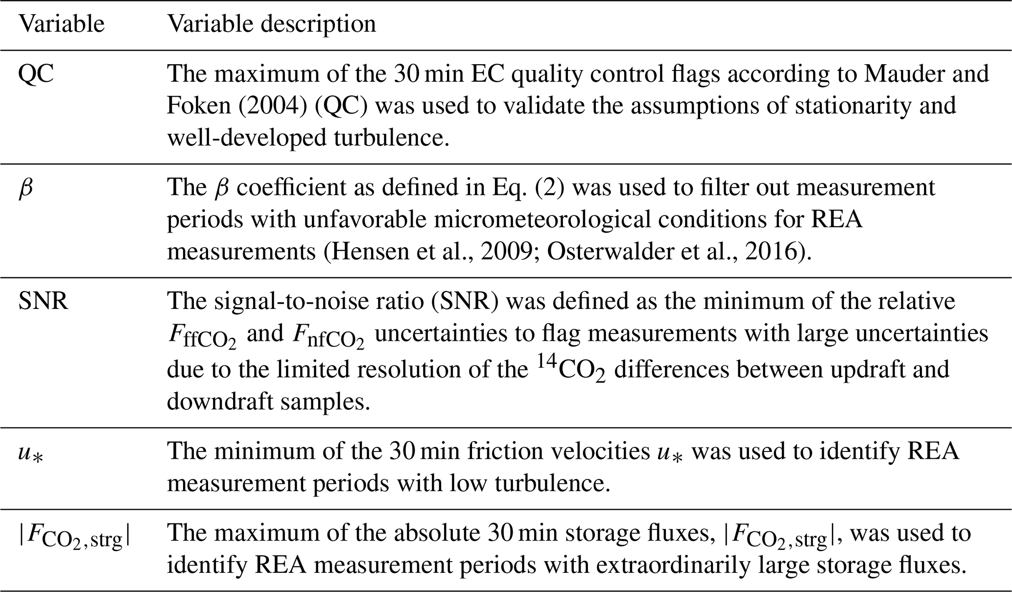
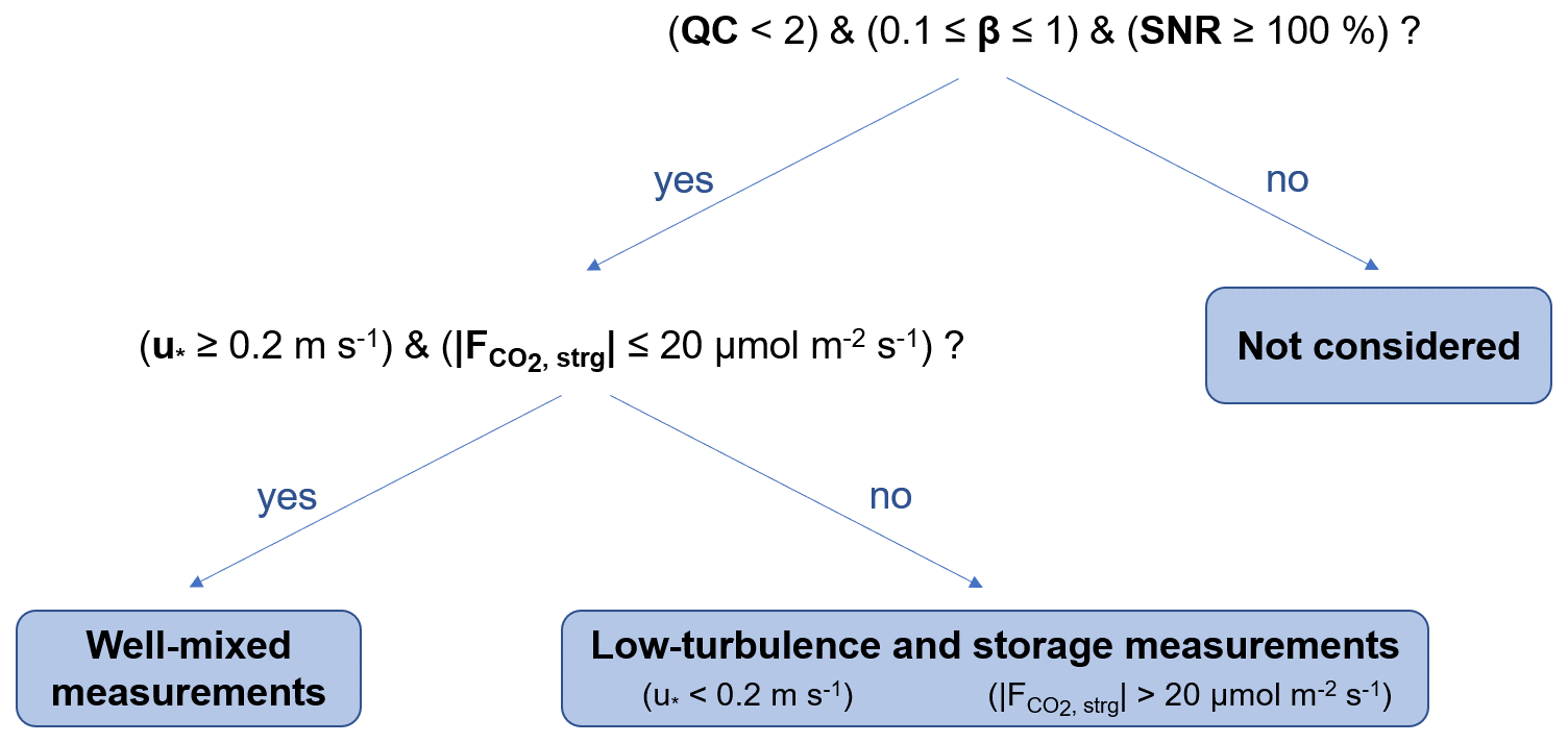
Besides technical requirements, REA is like any other turbulent flux measurement technique restricted to certain micrometeorological conditions, e.g., stationarity and well-developed turbulence (Rinne et al., 2021). Moreover, and in contrast to the EC technique, REA measurements cannot be processed retrospectively, e.g., cannot be corrected for changes in the mean vertical wind velocity. Therefore, additional criteria are necessary (Fotiadi et al., 2005a). Several criteria have already been considered in the selection of suitable flask samples during the campaigns (Kunz et al., 2025a). However, due to the limited number of good sampling conditions in the urban environment, the refinement of EC processing options, and the addition of further criteria after the measurement campaign, the analyzed sampling periods were not always ideal for REA measurements. For analysis of the results, the measurements were characterized based on five flagging criteria (Table 1, see Appendix B for details). Based on these criteria, the analyzed REA measurements were classified into three categories (Fig. 2). “Well-mixed measurements” are assumed to best represent the surface fluxes during the sampling period. These measurements are the most valuable for answering our research questions and were analyzed in the most detail. In contrast, “low-turbulence and storage measurements” are probably not representative of the surface fluxes during the sampling period due to insufficient turbulence or changes in storage below the measurement height (Sect. 2.2.1). However, the relative ffCO2 contributions were investigated to characterize the integrated fluxes before and during the sampling period. Measurements with QC =2, β<0.1, β>1 or SNR <100 % were not considered further in this study.
Mauder and Foken (2004)(Hensen et al., 2009; Osterwalder et al., 2016)Table 1Flagging criteria for analyzed REA measurements. See Appendix B for details.
2.3 Analysis of well-mixed REA measurements
2.3.1 Flux footprints and mean land cover fractions
To analyze the flux source areas during the individual REA measurements, flux footprints were derived for each 30 min averaging interval using the flux footprint model of Kljun et al. (2015). Inputs were turbulence data from eddy covariance measurements (ICOS Ecosystem Thematic Centre et al., 2025a, b, c; Ecosystem Thematic Centre, 2025), boundary layer height ERA5 reanalysis estimates from the Copernicus Climate Change Service (Hersbach et al., 2024), measurement heights and tower coordinates, and roughness length and displacement height derived from building and vegetation height maps. Details on the flux footprints are provided in Molinier and Kljun (2024).
For the 30 min time periods during which well-mixed REA measurements were taken, aggregated footprints were calculated. These aggregated footprints were combined with the WorldCover product provided by the European Space Agency (https://esa-worldcover.org, last access: 12 December 2025) to derive comparable mean land cover fractions using the same data source for each city. The flux footprints were also used to identify measurements which were potentially influenced by emissions from a district heating plant in Zurich and a brewery in Munich by calculating the expected flux contributions from the corresponding areas of interest (Appendix F).
2.3.2 Determination of mean ffCO2 CO2 flux ratios and evaluation of the significance of average nfCO2 flux components
To generalize and quantify the results from the individual REA measurements, the mean ffCO2 CO2 flux ratios and the mean magnitude of the nfCO2 fluxes were determined for each city. Due to the small number of measurements, it was not possible to fully account for the spatial and temporal variability. We distinguished between summer and winter measurements, and excluded measurements which were potentially influenced by large point-source emissions. In this work, “summer” refers to the period from July to October, and “winter” to the period from November to April (inclusive). This seasonal division of the measurement campaigns aligns roughly with the shift between European summer and winter time and with the change in local emissions due to heating degree days, and is consistent with other studies conducted in the same location during the same period (Hilland et al., 2025). If ffCO2 and CO2 fluxes were perfectly linearly correlated, the mean ffCO2 CO2 ratios would be best described by the slope of an error-weighted total least squares regression line (Maier et al., 2024a). Due to generally low correlations of the observed REA fluxes, however, was determined as the error-weighted mean of the individual ffCO2 CO2 ratios. To minimize the uncertainty, the individual values were calculated directly from the flask measurements as ΔffCO2 ΔCO2, i.e., completely independent of the EC flux measurements (compare Eq. 3). % indicates a negative nfCO2 flux, i.e., photosynthetic uptake, while % is physically unreasonable and only observed if ΔffCO2 is slightly negative within its measurements uncertainties. In addition, the mean and variability of the nfCO2 fluxes were examined. A z-test was used to evaluate whether the observations were significantly different from % or FnfCO2=0 µmol m−2 s−1 (significance level of 0.05), i.e., completely fossil CO2 fluxes, taking into account the mean measurement uncertainties. To meet the assumption of normal distribution, only measurements with relative ΔCO2 uncertainties ≪1 were considered (most, but not all, of these samples were already excluded by the consideration of the signal-to-noise ratio as defined in Sect. 2.2.4). See Appendix H for details.
2.3.3 Analysis of regional CO2 concentration enhancements
While the REA flask measurements aimed to analyze turbulent ffCO2 fluxes at the urban neighborhood scale, the absolute flask concentrations also contain information about the fossil and non-fossil CO2 enhancements compared to clean background air and thus about the composition of CO2 fluxes in a broader continental region, including other urban areas and regional emission sources. Following Levin et al. (2003), we calculated the ffCO2 excess from the mean CO2 and Δ14C values of the up- and downdraft REA sample pairs, using the corresponding concentration measurements at the European marine background station Mace Head on the western coast of Ireland as background concentrations, and assuming that the biogenic Δ14C signature equals the background concentration (see Appendix A2). Second-order effects, such as 14C-enriched heterotrophic respiration and nuclear contamination (Maier et al., 2023), were not considered because the necessary concentration footprints were only available until the end of 2023, and the corrections are negligible for our analysis. For details and an evaluation of these corrections on the Zurich measurements, we refer to Maier et al. (2023) and Appendix A2. The mean ffCO2 CO2 ratios of the excess concentrations thus represent the average contributions of ffCO2 emissions to the CO2 fluxes on the trajectories between Mace Head and the three measurement sites.
To assess the performance and to analyze the results of REA 14C measurements for different urban environments, the REA system as well as the EC systems (IRGASON and MGA7) were successively installed and operated for nine months each on three tall towers in the cities of Zurich, Paris, and Munich. The measurements were conducted as part of the ICOS Cities project (https://www.icos-cp.eu/projects/icos-cities, last access: 1 February 2026), at the same time and place as the studies by Lan et al. (2024), Stagakis et al. (2025), and Hilland et al. (2025). At each site, the gas inlets for updraft and downdraft sampling and the inlet for the MGA7 measurements were mounted on a mast on top of a high-rise building or tower about 20 cm apart from the ultrasonic anemometer and the open-path CO2 sensor of the IRGASON (Appendix C). The data logger, flask sampler, and the MGA7 were located in a climate controlled room. The intake line of the MGA7 was set up in the same way as the flask sampling lines. REA samples were typically collected over 60 min, starting every other hour. Since increased stability at night is unfavorable for REA measurements (Fotiadi et al., 2005a), flasks were sampled during the day only. To ensure reliable measurements from the open-path gas analyzer, samples collected during periods of low signal strength, i.e., rain events, were discarded. With growing experimental experience, the logger program, REA system, and selection criteria were progressively updated, while the overall methodology remained consistent across the three cities. A documentation and version history of the logger program is publicly available at https://doi.org/10.5281/zenodo.13926681 (Kunz et al., 2024). Despite non-idealities in the EC measurement setups, e.g., unfavorably long intake lines for the MGA7, spectral analysis and comparisons between the IRGASON and MGA7 data showed good quality of the EC flux measurements (Appendix D). In addition, the regular quality control tests of the REA system demonstrated an overall good performance of the REA hardware (Appendix E). Figure 3 shows the locations of the three measurement sites, along with the 10 %–80 % source areas for the well-mixed REA measurements. An overview of the site-specific data is provided in Table 2. For better readability, we refer to the three sites by their respective city names.
Table 2Site-specific data from the three REA measurement campaigns in Zurich, Paris, and Munich. δ and H are the scaling factors for the deadband width (REA) and the hole size (HREA), respectively. “Pre-set” and “dynamic” indicate whether the latter was fixed at the beginning of the sampling period or continuously adjusted based on the standard deviation of the vertical wind velocity. The numbers of successful samples and the numbers of successful samples selected and analyzed for 14C are listed; here, “successful” measurements refer to measurements in which enough sample air for laboratory analysis was collected in both the updraft and downdraft reservoirs. Land cover fractions within the aggregated footprints of the well-mixed REA measurements are given for the three main land cover types.
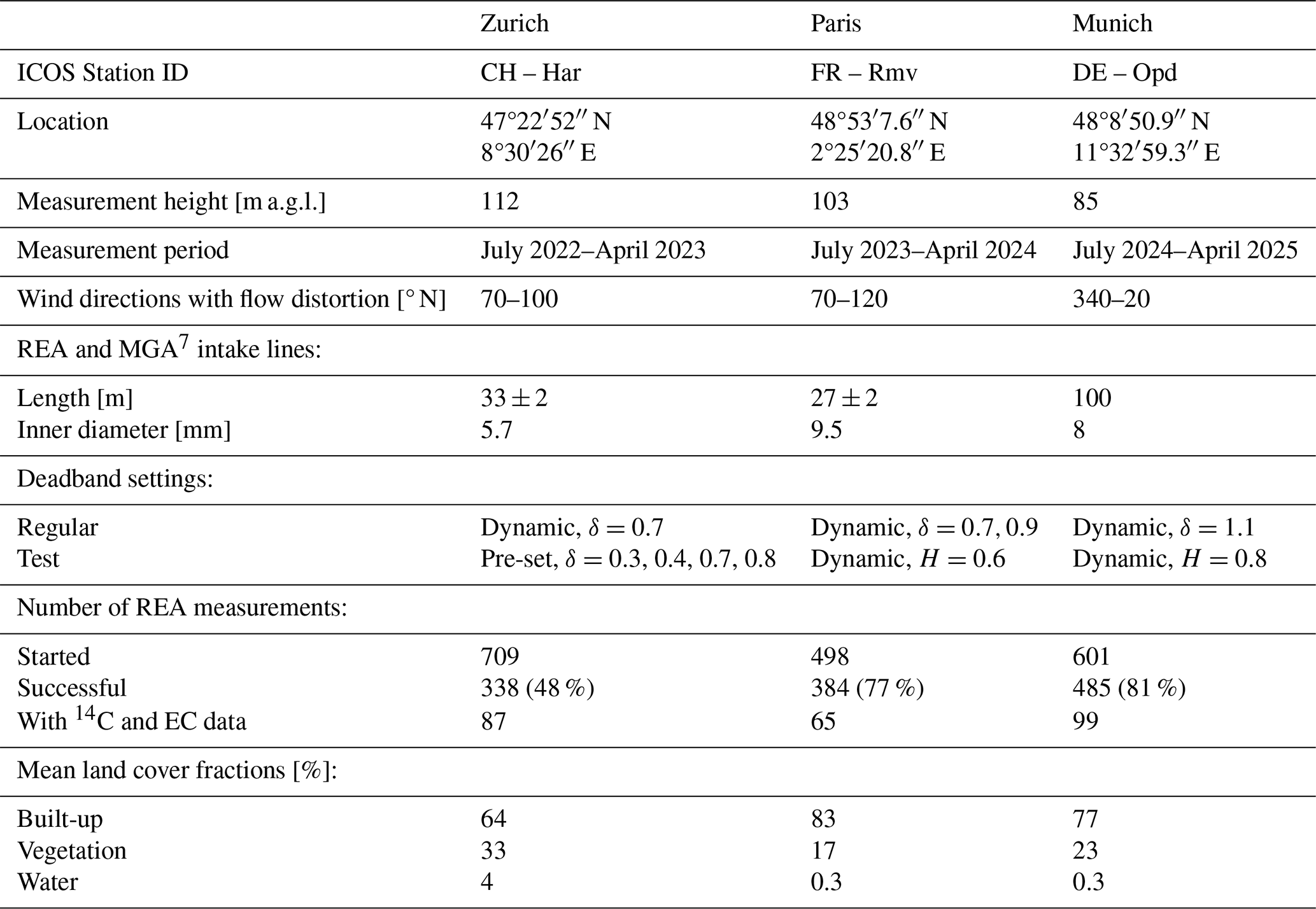
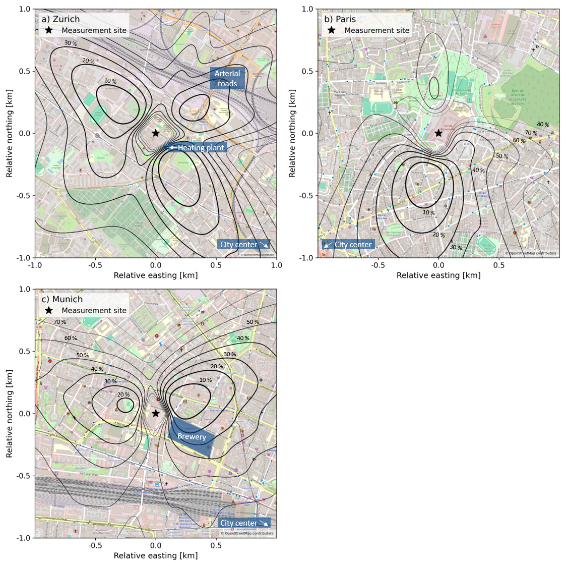
Figure 3Locations of the measurement sites in Zurich, Paris, and Munich, and aggregated flux footprints of the well-mixed REA measurements according to Kljun et al. (2015) (black contour lines). The depicted areas contributed an average of 10 %–80 % to the fluxes observed during REA measurements under well-mixed conditions. Map data from © OpenStreetMap contributors 2025. Distributed under the Open Data Commons Open Database License (ODbL) v1.0, https://www.openstreetmap.org/copyright.
3.1 Zurich – Hardau
In Zurich, the REA and EC measurements were conducted on an antenna of 16.5 m height on top of a 95.3 m high-rise building, i.e., approximately 112 m above ground level at the site Zurich – Hardau (ICOS Station ID “CH-Har”, Table 2, Fig. C1). The building, called Hardau II, is located roughly 1.5 km northwest of the city center of Zurich, Switzerland (Fig. 3a). It is surrounded by three similar buildings of lower height (66, 76, and 85 m). Apart from that, the average building height within a 1.5 km radius is 13.3±8 m. Located to the north are an industrial sector, railway lines, and busy arterial roads, to the west is a residential, green area with a cemetery, and to the southeast is an urban sector and the city center. Within the average flux footprint of the well-mixed REA measurements, about 64 % of the surface area is covered by built-up areas, 33 % by vegetation, and 4 % by water (Lake Zurich). The largest point source in the immediate vicinity, located 145 m southeast, is a district heating plant that uses natural gas.
During the first REA measurements in July 2022, different deadband settings (δ=0.3, 0.4, 0.7, and 0.8 with pre-set deadband) and averaging times (45, 60, 75 min) were tested (Table 2). With the pre-set deadband, in about 75 % of the REA measurements at least one of the reservoirs did not collect sufficient air to fill a flask. Therefore, a dynamic deadband with δ=0.7 was implemented and has been used since the end of August 2022. This was better suited for variable wind conditions and increased the percentage of successful measurements to 75 %. Unfortunately, all samples collected between November 2022 and February 2023 had to be discarded due to a leak in the REA sampler, which was detected retrospectively. More details on the Zurich measurements are given in Kunz et al. (2025a).
3.2 Paris – Romainville
In Paris, the REA and EC systems were installed on an active telecommunications tower about 5 km northeast from the city center at the site Paris-Romainville (ICOS Station ID “FR-Rmv”, Table 2). The IRGASON and the gas inlets were mounted on a pylon, approximately 9 m above a wide (∼ 30 m) platform (Fig. C1). Due to the massive structure of the tower, flow distortion effects were observed between 70 and 120° N. The tower is located on a small hill in a densely urbanized area (Fig. 3b). The average flux footprint of the well-mixed measurements was clearly dominated by built-up areas, with only 17 % of the area being vegetated.
Between July 2023 and April 2024, 66 of 384 successful and 498 scheduled REA measurements were analyzed in the laboratory. One sample was rejected due to abnormal 12C currents during 14C analysis at the accelerator mass spectrometer (AMS), as well as implausible measurement results, leaving 65 REA measurements with 14C and EC data (Table 2). To minimize wind distortion effects, no samples were collected from wind directions between 70 and 120° N. For the vast majority of the analyzed samples, the mean wind direction was between 180 and 225° N. The deadband was initially scaled with δ=0.7, as in Zurich, but was increased to δ=0.9 in October 2023 due to very small concentration differences between updrafts and downdrafts. With a pump speed of about 7 L min−1, this was the maximum possible deadband width to collect sufficient air during a 60 min sampling period. Since the concentration differences were still close to the detection limit, the option for HREA was implemented in the logger program (Sect. 2.2) at the beginning of April 2024. To test the HREA method, nine samples were collected with H=0.6. Due to technical problems with the MGA7 in 2023, only EC measurements of the IRGASON are available for 2023. Between November 2023 and January 2024, the MGA7 was dismantled for repairs and no REA measurements were conducted.
3.3 Munich – Oberpostdirektion
From July 2024 to April 2025, REA measurements were carried out on a mast of an active telecommunications tower about 1.5 km northwest of the city center of Munich at the site Munich-Operpostdirektion (ICOS Station ID “DE-Opd”, Table 2). The tower has three platforms up to a height of 59 m and a mast on top, on which the IRGASON and the gas inlets were mounted at a height of 85 m (Fig. C1). In addition, two mid-cost sensor systems, which are based on the Non-Dispersive InfraRed CO2 sensors GMP343, Vaisala Oyj, Vantaa, Finland, measured the CO2 concentration at heights of 85 and 48 m (part of the Munich mid-cost network ACROPOLIS (Aigner et al., 2026)). The tower is located in an area with many residential houses and other buildings (Fig. 3c). To the southeast is the central railway station and behind it the historic city center. The largest point source, located approximately 200 m to the southeast, is a brewery. Vegetation accounted for approximately 23 % of the average flux footprint area of the well-mixed REA measurements.
Due to lack of space, the MGA7 and the REA sampler were placed in the basement of the tower, requiring inlet lines of 100 m length. During the maintenance of the REA system prior to its installation in Munich, larger flushing pumps were installed (Sect. 2.2). The sampling flow rate was increased to approximately 11 L min−1. With the increased flow rate, less time was needed to collect enough air for laboratory analysis, so a larger deadband (δ=1.1) could be used. For summer afternoons with predominantly small CO2 fluxes, a hyperbolic deadband with hole size H=0.8 was used to increase the signal-to-noise ratio.
4.1 Flagging of analyzed REA measurements
The quality of a collected REA data set strongly depends on site-specific conditions such as flux strength or micrometeorological conditions, technical settings such as the deadband, and the data and knowledge available during the campaign for the selection of suitable flask samples adapted to the scientific question. In our case, the largest number of high-quality ffCO2 flux data could be collected in Munich.
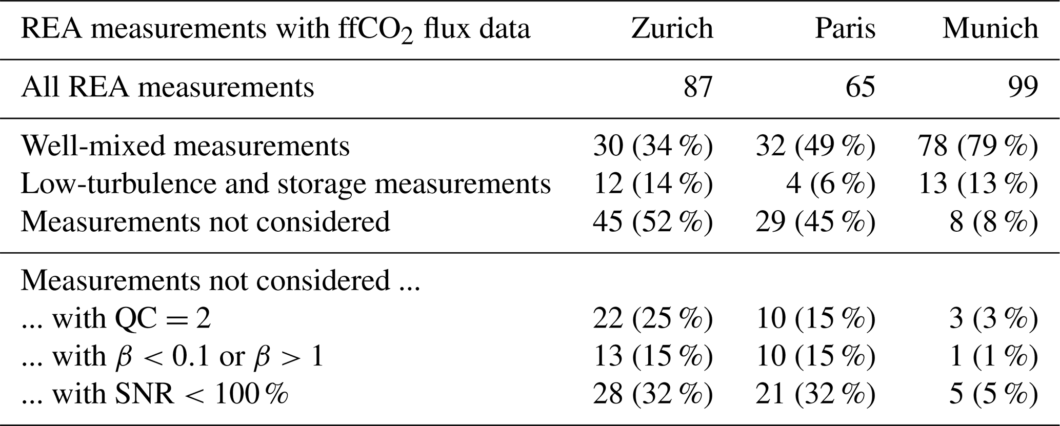
Table 3Number of well-mixed measurements, low-turbulence and storage measurements, or measurements not considered further (Fig. 2). In brackets, the percentages of the total number of REA measurements with ffCO2 flux data are provided. For the measurements not considered further, the individual numbers and percentages for each flagging criterion are also given. These measurements may be affected by multiple criteria. Quality control flag QC, beta coefficient β, and signal-to-noise ratio SNR are defined as in Table 1.
In Zurich, only 30 out of 87 REA measurements with 14C and EC data were flagged as well-mixed measurements (Table 3). Twelve samples were selected knowing that with m s−1 or µmol m−2 s−1 the measurements probably did not represent the surface fluxes during the sampling period. Most of these measurements with low-turbulence or storage flag were taken in the early morning and analyzed to obtain information on the composition of the nocturnal CO2 fluxes. As it was initially decided to relax the stationarity requirements due to the intermittent nature of CO2 fluxes in urban environments, 25 % of the periods did not meet the stationarity or well-developed turbulence criteria. The β criterion was not considered in the selection of the flasks, but only 15 % of the measurements were affected. Excluding measurements with β<0.1, β>1 and QC =2, β was 0.44±0.14 for a dynamically adjusted deadband width of 0.7σw. This is slightly higher than the value of 0.39, which would be expected for a normally distributed timeseries with δ=0.7 (Fotiadi et al., 2005b), but in good agreement with experimental data (e.g., Pattey et al., 1993; von der Heyden et al., 2022) (see Appendix B2). The main limitation of the Zurich REA measurements was a signal-to-noise ratio of <100 %, caused by the small Δ14C differences between updraft and downdraft samples compared to the mean measurement uncertainty of the Zurich samples of 1.8 ‰ (Δ notation according to Stuiver and Polach, 1977). In Paris, low-turbulence and storage measurements were usually not selected for laboratory analysis. The β coefficient for δ=0.7 was 0.40±0.20, i.e., slightly smaller than in Zurich and in good agreement with theoretical expectations for normally distributed time series. Unfortunately, increasing δ to 0.9 did not increase the concentration differences. For the selected measurements, β was even slightly larger on average (0.46±0.17, see Appendix B2). As in Zurich, the main limitation of the measurements in Paris was a low signal-to-noise ratio. In Munich, the proportion of suitable measurements was significantly improved. The concentration differences were generally increased by a larger deadband width and HREA. The β coefficient was 0.34±0.07 for a deadband with δ=1.1 and 0.26±0.06 in the case of HREA with H=0.8, i.e., as expected much smaller than in Zurich and Paris (Appendix B2). At the same time, the Δ14C measurement uncertainties were reduced by a new AMS from 2.1±0.3 ‰ (Zurich samples with old AMS) to 1.2±0.1 ‰, so that samples with SNR >100 % could be selected. As in Zurich, low-turbulence and storage samples collected in the morning were deliberately selected to analyze the ffCO2 CO2 ratio of nocturnal integrated fluxes. In all three cities, storage flux estimates for the well-mixed measurements were on average less than 5 % of the absolute CO2 fluxes, which justifies the neglect of storage flux corrections for the selected measurement periods. An overview of all REA measurements and their corresponding flags can be found in Kunz et al. (2025b).
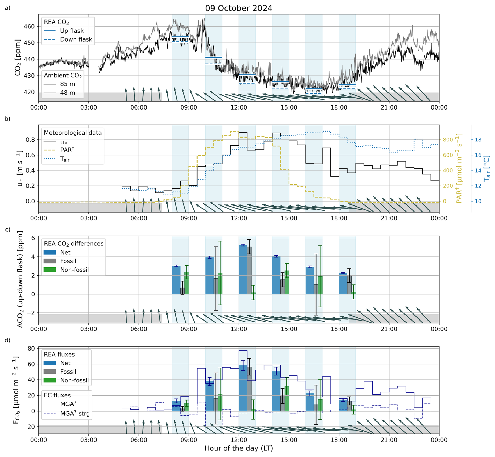
Figure 4Visualization of EC and REA measurements on 9 October 2024 in Munich. Sampling periods of the six REA measurements are highlighted in blue. Arrows at the bottom of the plots indicate the mean horizontal wind direction and wind speed over 30 min. Day and night times are indicated by the gray bar. (a) CO2 in situ measurements of the GMP343 at 85 m (= REA sampling height) and 48 m together with CO2 concentrations of the updraft and downdraft flask samples. (b) 30 min averages of friction velocity u*, photosynthetically active radiation PAR and air temperature Tair (†PAR was approximated by 1.7 µmol J−1 times the average incoming shortwave radiation). (c) CO2 concentration differences between updraft and downdraft flask samples ΔCO2 and their fossil and non-fossil components derived from the respective 14CO2 measurements. (d) Continuous CO2 flux and CO2 storage flux estimates from EC measurements of the MGA7 with 30 min averaging period. Blue bars indicate the mean net CO2 fluxes during the REA sampling periods, gray and green bars the respective fossil and non-fossil components derived from the flask concentration differences.
4.2 Example diurnal course
On 10 October 2024, favorable micrometeorological conditions enabled repeated REA measurements in Munich throughout the day. All six flask pairs sampled between 08:00 and 19:00 local time (LT = UTC+2) were analyzed for 14CO2. The exemplary analysis of the measured ffCO2 and nfCO2 fluxes demonstrates the successful separation of net EC CO2 fluxes using REA for 14CO2 and its benefits. However, the analysis also highlights the challenges and limitations in interpreting and generalizing the data, which arise from the observed variability in the CO2 flux composition, the overall sparse data coverage, and the large measurement uncertainties.
The CO2 concentration of ambient air, as measured by the two mid-cost sensor systems at 48 m above ground level (Fig. 4a), followed the typical diurnal CO2 cycle of a warm and sunny summer day (e.g., Stull, 1988; Lan et al., 2020). During night, the CO2 concentration increased and a vertical concentration gradient with highest values close to the surface developed. As vertical mixing was suppressed ( m s−1, see Fig. 4b), this can be attributed to surface emissions accumulating within the stable nocturnal boundary layer. After sunrise, friction velocity, temperature, and radiation increased (Fig. 4b). As the radiative heating of the surface generates convective turbulent vertical motions, the vertical concentration gradient diminished. The CO2 concentration decreased at both heights first rapidly due to the entrainment of fresh air from higher altitudes, then more slowly as the depth of the atmospheric boundary layer stabilized and changes in CO2 concentration were primarily driven by the surface fluxes.
The net CO2 flux, on the contrary, did not follow the typical, traffic-dominated, bimodal diurnal cycle that might be expected in the urban environment. Instead, it peaked around noon (Fig. 4d). Accordingly, the net CO2 concentration differences between the sampled updraft and downdraft flasks were also largest during the measurement between 12:00 and 13:00 (Fig. 4c). However, the 14C-based ΔffCO2 estimates (Fig. 4c) provide additional information on the composition of the measured fluxes. At noon and in the evening, the net CO2 differences, and thus also the net CO2 fluxes, were entirely caused by fossil fuel emissions. Consequently, the ffCO2 flux was equal to the net EC-based CO2 flux, while the nfCO2 flux was approximately zero. It should be noted that does not necessarily mean that there was no biospheric activity, but only that the positive fluxes (respiration + biofuels) were approximately equal to the photosynthetic uptake. In the morning and in the afternoon, on the other hand, the ΔffCO2 ΔCO2 ratio, and thus also the ratio, varied between 23 % and 43 %, indicating positive nfCO2 fluxes of about 10 to 30 µmol m−2 s−1. For an urban environment, nfCO2 fluxes of 30 µmol m−2 s−1 are extraordinarily large. As shown in Sect. 4.3.2, such high nfCO2 fluxes were repeatedly observed from the southeast, indicating emissions from a real nfCO2 source and an appropriate measurement principle capable of detecting such signals. For the REA measurements in the early morning, it is important to recall that the EC and REA data represent the turbulent fluxes and are not corrected for changes in storage below the measurement height (Sect. 2.2.1). This is particularly relevant for the measurement at 08:00, where m s−1 and the CO2 concentration at 48 m was higher than at 85 m. Due to low turbulence, the measurement may not reflect the surface fluxes at the actual time of sampling. Indeed, the ffCO2 CO2 flux ratio of 22 ± 23 % is much lower than expected during the morning rush hour. Although the measurement at 10:00 was flagged as well-mixed, the decrease in CO2 concentration, the negative storage flux estimate, and the relatively high nfCO2 contribution (neglecting uncertainties) also indicate a storage contribution, i.e., mixed-up near-surface accumulation from the previous night. This highlights that the 20 µmol m−2 s−1 threshold flags only the most extreme storage flux measurements, and that the flagging is not unambiguous, especially given the high uncertainty in the storage flux estimates in the morning. Since storage fluxes are usually largest in the morning, the well-mixed measurements were additionally analyzed for differences between measurements taken before and after 11:00 LT (Sect. 4.3.3). Unfortunately, the ΔffCO2 uncertainties for the REA measurements at 10:00 and 16:00 were unusually high due to technical issues during the 14CO2 AMS measurements in the subsequent lab analysis.
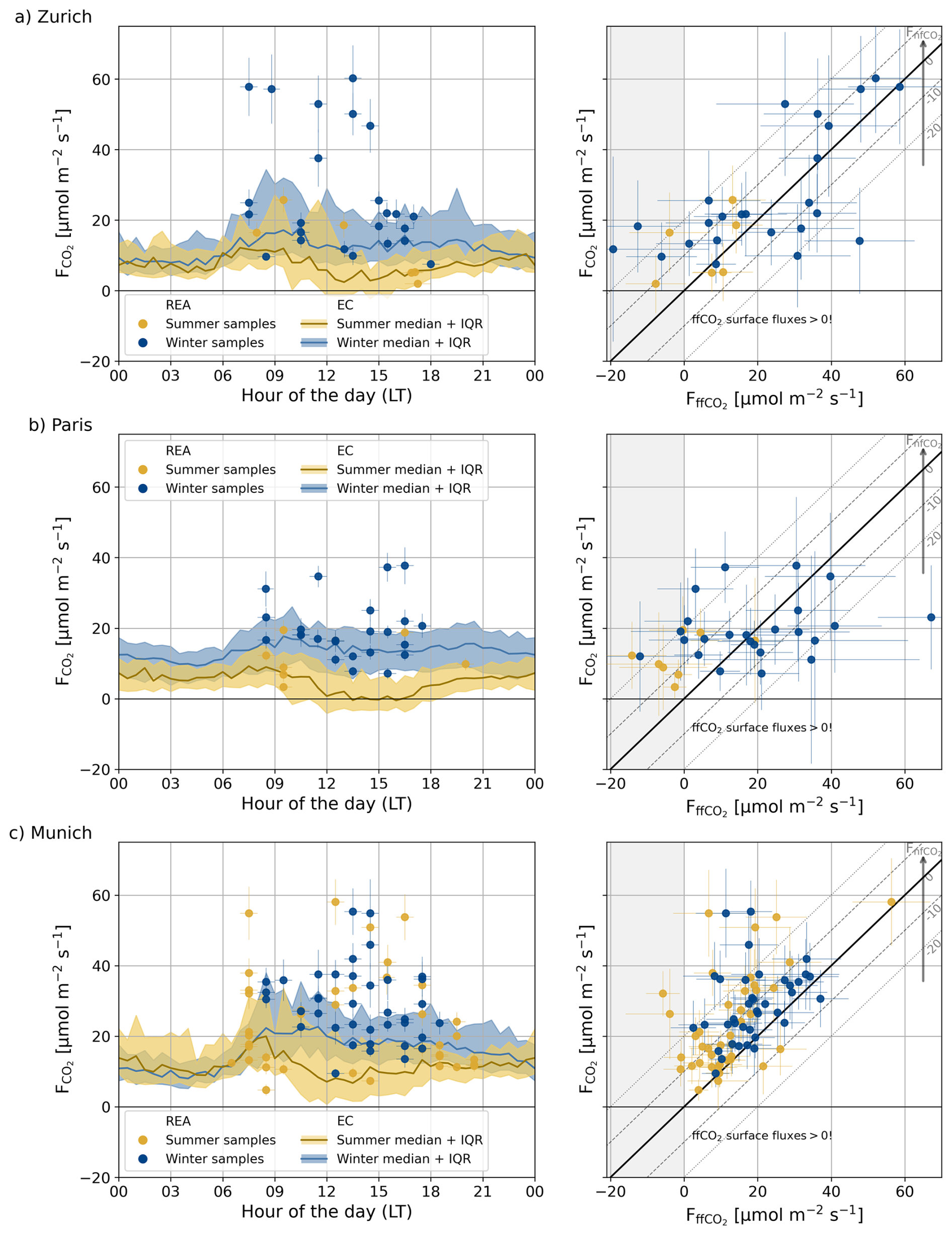
Figure 5Overview of all REA measurements in Zurich, Paris, and Munich with well-mixed conditions. Left: Net CO2 flux during the REA sampling periods over the hour of the day. Error bars in x-direction indicate the length of the REA sampling period (mostly 60 min), error bars in y-direction the uncertainty of . The yellow and blue lines and shaded areas represent the medians and the interquartile ranges (IQR) of the continuous IRGASON CO2 fluxes (see Appendix D for details). Right: CO2 fluxes during the REA sampling periods compared to the 14C-based ffCO2 fluxes. The areas with are shaded gray because the physical ffCO2 fluxes at the surface are positive. The magnitude of the nfCO2 flux is indicated by the parallel dashed lines and the axes on the right. Error bars in x-direction represent uncertainties, error bars in y-direction represent uncertainties.
4.3 Partitioning of net CO2 fluxes under well-mixed conditions
4.3.1 Overview of sampling times and ffCO2 vs. CO2 fluxes from all three cities
A qualitative analysis of the observed ffCO2 fluxes from the well-mixed REA measurements, in relation to net CO2 fluxes and the time of day (Fig. 5), shows that due to the selection of samples with large SNR the dataset is biased towards high fluxes. While the large CO2 fluxes clearly differed in composition between the three sites, the separation of smaller fluxes was limited by measurement uncertainties, particularly in Zurich and Paris.
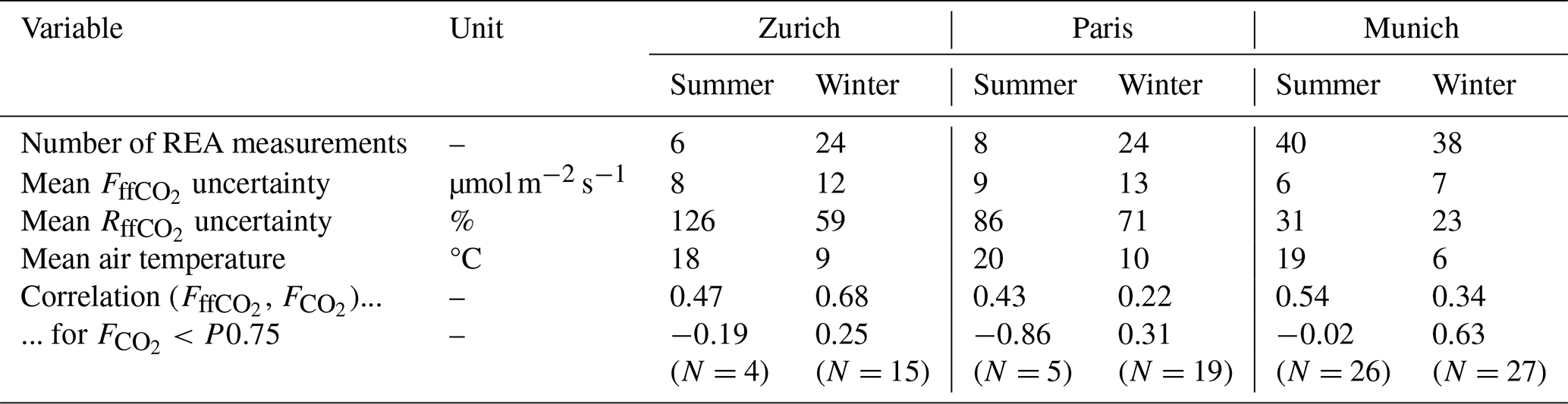
The continuous EC measurements showed that the CO2 fluxes were, on average, as expected higher in winter than in summer, especially during the day, pointing at increased emissions and reduced photosynthetic uptake. The differences were most pronounced in Paris, where in summer the median turbulent flux between 12:00 and 17:00 LT was approximately zero. This means that in 50 % of the considered time periods, negative CO2 fluxes, i.e., photosynthesis, were larger than positive CO2 fluxes through respiration and anthropogenic emissions. Seasonal differences are also evident in the REA ffCO2 measurements. In Zurich and Paris, ffCO2 fluxes were, on average, much smaller in summer than in winter. However, the representativity of the results is limited by the small number of well-mixed measurements, particularly in summer. It should also be noted that negative ffCO2 surface fluxes are unreasonable and are attributed to the limited resolution of small 14CO2 differences between updraft and downdraft samples (the error bars indicate the 1σ uncertainties). Nevertheless, the measurements are shown here, because they have a significant nfCO2 component (SNR >100 %). The fact that far fewer negative ffCO2 flux data points were measured in Munich than in Zurich and Paris highlights the improvement in the REA measurements in Munich. In Munich, the difference between summer and winter measurements was much smaller, despite comparable mean air temperatures during the REA measurements to those in Zurich and Paris (Table 4). This could be related to the relatively large proportion of buildings in the footprint of the Munich tower that are heated by district heating.
Compared to the median CO2 fluxes, the fluxes during the selected REA sampling periods were often exceptionally high. This indicates that the dataset is biased towards high fluxes, caused by the systematic selection of flask pairs with large CO2 concentration differences to increase the potential ffCO2 signal. In Zurich, all of the analyzed fluxes that exceeded the 75th percentile of the continuous EC fluxes (denoted as P0.75 in the following) were measured in winter and were almost entirely due to fossil fuel emissions. In Paris, there were only five REA measurements with . As in Zurich, they were measured in winter, but they were not as clearly dominated by fossil fuel emissions as the large winter fluxes measured in Zurich. In Munich, turbulent fluxes >P0.75 were analyzed in both summer and winter, and most had a significant positive nfCO2 component. Thus, while the large fluxes represent relatively rare conditions, the high signal-to-noise ratio (which was the main reason for analyzing them) allows observation of differences in the composition of the fluxes between the three cities (cf. Sect. 4.3.2 and 4.3.3).
REA measurements conducted in Zurich and Paris when CO2 fluxes were below P0.75 showed positive and negative nfCO2 components of up to ±45 µmol m−2 s−1. However, the uncertainties were large and there were very few summer measurements, as most of the measurements were flagged because of SNR <100 %, β<0.1 or β>1. In Munich, on the contrary, the uncertainties were much smaller (see Table 4) and, except for a few measurements, all measurements showed positive nfCO2 components. This means that respiration and biofuel emissions were generally larger than photosynthetic uptake. The latter is consistent with the observations from the continuous EC measurements that the net CO2 fluxes were highest in Munich and mostly positive throughout the year.
The correlation between the ffCO2 and CO2 fluxes was largest (0.68) for the Zurich winter measurements (Table 4). However, no clear correlation was observed when only the measurements with were considered. This could be caused by a large biospheric signal, a large temporal or spatial variability and/or an insufficient signal-to-noise ratio. To investigate the cause more closely, spatial patterns and expected effects of measurement uncertainties are discussed in Sect. 4.3.2 and 4.3.3.
Table 4Mean uncertainties of the ffCO2 fluxes and the ffCO2 CO2 flux ratios of the REA measurements under well-mixed conditions in Zurich, Paris, and Munich. In addition, the Pearson correlation coefficients of the ffCO2 and CO2 fluxes and the mean air temperatures during the sampling periods are given. P0.75 denotes the 75th percentile of the continuous EC CO2 fluxes.
4.3.2 Spatial flux patterns and influence from large point-source emissions
Extraordinarily large CO2 fluxes analyzed in Zurich and Munich showed different compositions (Sect. 4.3.1). While the Zurich fluxes were mostly fossil, the Munich fluxes contained a surprisingly large nfCO2 component. Based on the mean wind directions and modeled flux footprints, we found that these measurements were likely affected by fossil fuel emissions from a district heating plant in Zurich and non-fossil emissions from a fermentation process in a brewery in Munich, respectively. The conclusive results indicate high quality of the REA and EC measurements, and the footprint analysis. Moreover, these point-source influenced measurements highlight the challenges involved in interpreting atmospheric observations in a complex urban environment.
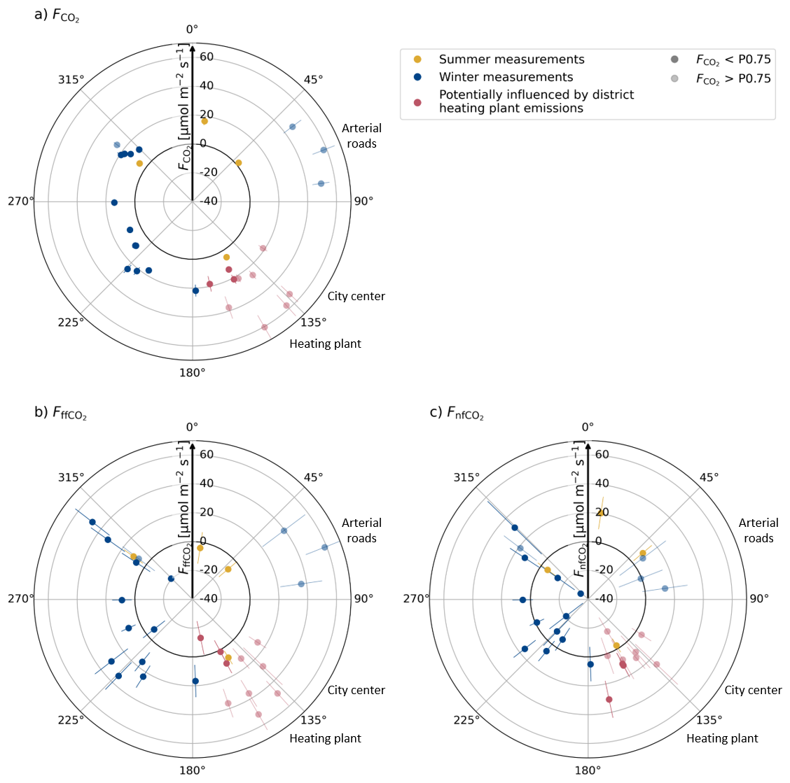
Figure 6Net CO2 fluxes (a), ffCO2 fluxes (b), and nfCO2 fluxes (c) with respect to the mean wind directions during the measurement intervals in Zurich with well-mixed conditions. The error bars represent the respective flux uncertainties. Measurements potentially influenced by emissions from a district heating plant to the southeast are indicated in red. P0.75 denotes the 75th percentile of the continuous EC CO2 fluxes at the respective hour of the day of the respective season. Indicated are also the directions of the arterial roads, the city center, and the district heating plant.
In Zurich, the net CO2 fluxes observed with wind from the west were generally smaller than those with wind from the east (Fig. 6a). The CO2 fluxes >P0.75, which were clearly dominated by fossil fuel emissions (Fig. 6b), were observed from about 70 and 135° N. This is consistent with the high proportion of vegetated areas in the west, in contrast to the city center, a district heating plant, and arterial roads in the east (Sect. 3.1). Based on analysis of the flux footprints and the operating times of the district heating plant, we identified 10 measurements from the southeast that were potentially influenced by emissions from the district heating plant. See Appendix F for details.
In Paris, measurements were primarily taken during south-southwesterly wind. Due to the sparse data coverage, no spatial patterns could be investigated. There is no evidence of any distinct point-source emissions that could have affected the REA measurements. For completeness, the corresponding directional figures for Paris are shown in Appendix G.
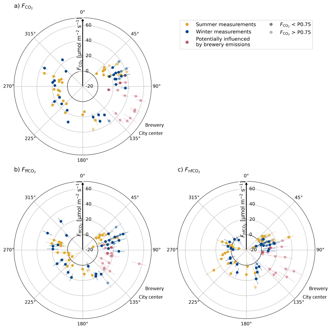
Figure 7Net CO2 fluxes (a), ffCO2 fluxes (b), and nfCO2 fluxes (c) with respect to the mean wind directions during the measurement intervals in Munich with well-mixed conditions. The error bars represent the respective flux uncertainties. Measurements potentially influenced by emissions from a district heating plant to the southeast are indicated in red. P0.75 denotes the 75th percentile of the continuous EC CO2 fluxes at the respective hour of the day. Indicated are also the directions of the brewery and the city center.
In Munich (Fig. 7), the highest CO2 fluxes were measured when the wind came from southeast-east. Located in this direction are a brewery, the central railway station, and the historic city center (∼0.3, 1, and 2 km horizontal distance, respectively, see Sect. 3.3). Striking are the large nfCO2 fluxes of up to 50 µmol m−2 s−1. The fact that biospheric and human respiration fluxes are typically much smaller (e.g., Wu et al., 2022; Stagakis et al., 2023b, 2025) indicates a non-respiratory anthropogenic nfCO2 source. Footprint analyses of the respective measurements, using the model of Kljun et al. (2015), showed that the brewery was within the peak area of the flux footprint (Appendix F). Therefore, we assume that the large nfCO2 emissions from the southeast-east resulted from a fermentation process (Elshani et al., 2018; Olajire, 2020). As there is no information available regarding operating times or the temporal emission profile of the brewery, all measurements with a substantial flux contribution from the brewery area, as estimated from the flux footprints, were considered to be potentially influenced by these large non-fossil point-source emissions (see Appendix F). Apart from measurements from the southeast, all nfCO2 fluxes >20 µmol m−2 s−1 were measured in the early morning. As discussed in Sect. 4.2, this could indicate an unaccounted contribution from storage fluxes, further supported by the uncertainties in the distinction between low-turbulence/storage and well-mixed conditions (Sect. 4.4).
The measurements provide confidence in the EC and REA measurements as well as in the footprint analysis, and could be used to validate or refine bottom-up emission estimates of the respective point sources. Non-fossil CO2 emissions from fermentation processes in breweries, for example, are usually not included in emission inventories. For the characterization of the usually smaller CO2 fluxes and the analysis of the biospheric nfCO2 fluxes, however, these measurements need to be excluded.
4.3.3 Mean ffCO2 CO2 ratios and mean nfCO2 fluxes
When the measurements potentially influenced by the large CO2 emissions from a district heating plant and a brewery near the measurement sites in Zurich and Munich were excluded, the error-weighted mean ffCO2 CO2 flux ratios of the well-mixed measurements were approximately 50 % or less in summer and 80 % to 90 % in winter. In Zurich and Paris, however, the significance and representativeness of the results were limited by the small number of measurements. In Munich, on the contrary, average nfCO2 contributions were significantly greater than zero, particularly in the early morning in summer. This highlights the improvements achieved in the REA measurements and the importance of considering nfCO2 fluxes in cities.
Table 5Error-weighted mean ffCO2 CO2 flux ratio and error-weighted mean nfCO2 flux of the well-mixed REA measurements, excluding measurements in Zurich and Munich, which were potentially influenced by identified point-source emissions, and four measurements with ΔCO2<0.4 ppm. N is the number of samples. Stars indicate that, given the number of measurements and mean measurement uncertainties, the results are significantly different from % or µmol m−2 s−1, respectively (, , ).
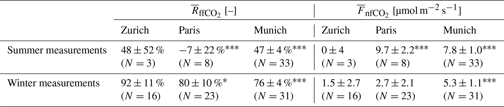
In Zurich, no significant average nfCO2 signal (p-values >0.05) was observed. In summer, the mean ffCO2 CO2 flux ratio was 48±52 % and the mean absolute nfCO2 flux was 0±4 µmol m−2 s−1. The significance of the results was mainly limited by the small number of well-mixed measurements (N=3). In winter, the mean ffCO2 contribution of the Zurich samples was 92±11 %. To resolve the presumably small mean nfCO2 component, many more measurements and/or smaller measurement uncertainties would have been necessary (see Appendix H).
In Paris, the eight selected summer samples showed mostly non-fossil CO2 contributions. The negative mean ffCO2 ratio could be explained by the ffCO2 flux uncertainties (compare Fig. 5), but a larger ffCO2 contribution was expected. Note that most of the measurements were conducted in the early morning. Therefore, storage fluxes cannot be ruled out. However, due to the small number of samples, a further subdivision of the measurements into morning and afternoon measurements, for example, was not feasible. Similar to the Zurich measurements, the Paris measurements were generally more successful in winter than in summer due to larger signals. The mean ffCO2 contribution in winter was 80±10 %, meaning that, on average, about 20 % of the observed CO2 emissions were due to positive nfCO2 fluxes.
In Munich, the higher data quality and greater number of measurements enabled the detection of significant nfCO2 contributions in both summer and winter. The larger nfCO2 fluxes observed in summer compared to winter were primarily attributed to the measurements taken in the early morning during summer. When only 18 summer measurements taken after 11:00 LT were considered, was 64±6 % and was 5.6±1.3 µmol m−2 s−1, which is much smaller than for the early-morning measurements and comparable to the winter measurements. In winter, no significant differences were observed between measurements taken before and after 11:00 LT. This could be explained by larger respiratory fluxes and nfCO2 dominated storage fluxes in the morning (Sect. 4.4) and larger photosynthetic uptake, i.e., negative nfCO2 fluxes in the afternoon. This temporal variability is larger in summer than in winter. With the reduced measurement uncertainties, about 50 to 100 REA measurements are sufficient to identify average nfCO2 fluxes of the order of 10 % or 3 µmol m−2 s−1 at a 0.05 significance level (Appendix H).
Overall, it is remarkable that the mean nfCO2 contributions are positive in all three cities, both in summer and in winter. Only a few measurements show a significant negative nfCO2 flux. This contrasts with various studies that estimated negative nfCO2 fluxes in urban areas, particularly during the warm growing season but also during the cold dormant season (e.g., Wu et al., 2022; Miller et al., 2020). The positive nfCO2 fluxes in our study could be explained, for example, by the low proportion of vegetated area within the flux footprints. However, the differences in between the three cities could not be attributed to the respective average vegetated area, which was slightly larger in Zurich than in Paris and Munich (Table 2). It should be noted that the observed nfCO2 fluxes include human respiration. According to bottom-up estimates for 2022, the mean annual human respiration fluxes within a 2×2 km2 square around the measurement sites are about 2.5 µmol m−2 s−1, or 10 % of the net CO2 fluxes in all three cities (Dröge et al., 2024). For comparison, the estimated human respiration flux in the footprint of the study by Wu et al. (2022) was only 0.22 µmol m−2 s−1. Human respiration could therefore account for a significant proportion of the observed nfCO2 fluxes. Moreover, due to the small number of analyzed samples and the systematic selection of samples with presumably large concentration differences, the results may be biased toward periods with positive nfCO2 fluxes. As a further analysis, a 1:1 comparison of the REA fluxes with the emission inventories and biospheric models, taking into account the respective flux footprints, could be useful. As the example of the high nfCO2 fluxes from the direction of a brewery in Munich shows, the measurements could also be influenced by other anthropogenic nfCO2 point sources. In Munich, for instance, there are also other, more distant breweries. Based on our flux footprint analysis, we excluded all measurements where one of these breweries could have impacted the measured flux. However, excluding these measurements had no significant impact on the results (not shown here). Consistent with the aforementioned studies, our measurements underscore the importance of nfCO2 fluxes in urban areas.
4.4 Low-turbulence and storage measurements
Although the low-turbulence and storage samples were collected under very different conditions, i.e., in different cities, with variable contributions from surface and storage fluxes, at different times of the year, etc., the ffCO2 CO2 flux ratios were mostly <70 % and larger during cold temperatures than during warm temperatures (Fig. 8). As the low-turbulence and storage measurements are assumed to contain information about the fluxes prior to the measurement period, the increased nfCO2 contribution in the morning measurements is most likely due to reduced traffic emissions at night, as well as no heating emissions and increased biospheric respiration, particularly in summer.
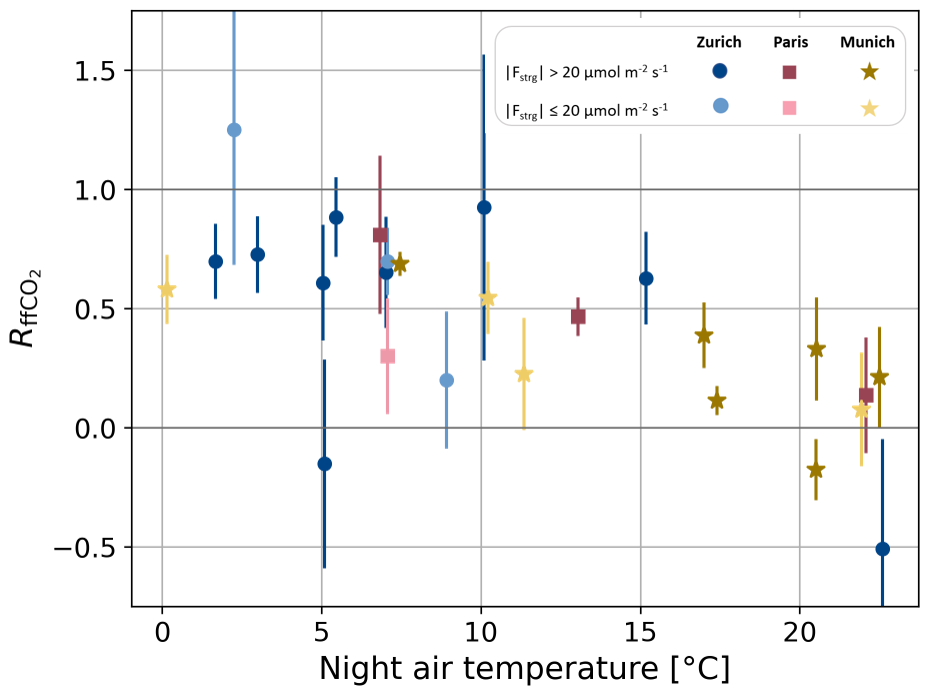
Figure 8ffCO2 CO2 flux ratios () of the low-turbulence and storage measurements taken before 11:00 UTC. The colors indicate whether µmol m−2 s−1 (storage flag) or µmol m−2 s−1 (low-turbulence flag only). The error bars represent the measurement uncertainties. The x-axis shows the mean air temperature between 00:00 and 06:00 UTC on the respective days.
In Zurich, the error-weighted mean ffCO2 CO2 flux ratio of the samples with night-time temperatures <10 °C was 68±7 %. This indicates that the surface fluxes, as well as the accumulation of CO2 in the stable nocturnal boundary layer, were primarily caused by fossil fuel emissions, e.g., due to building emissions, traffic, or industrial processes. However, there was also a substantial nfCO2 contribution of about 30 % or more in winter. The samples collected in Munich with night temperatures >10 °C showed a much lower mean ffCO2 CO2 ratio of 16±4 %.
The results are in good agreement with other studies. Moriwaki et al. (2006) attributed the nocturnal build-up of CO2 in a suburban canopy layer in winter to the subsidence of (fossil) building emissions. Wu et al. (2022) observed nocturnal ffCO2 CO2 flux ratios in Indianapolis of ∼66 % in winter and ∼33 % in summer. In general, nocturnal net ecosystem exchange is found to be much larger in summer than in winter (e.g., Crawford and Christen, 2015; Stagakis et al., 2025).
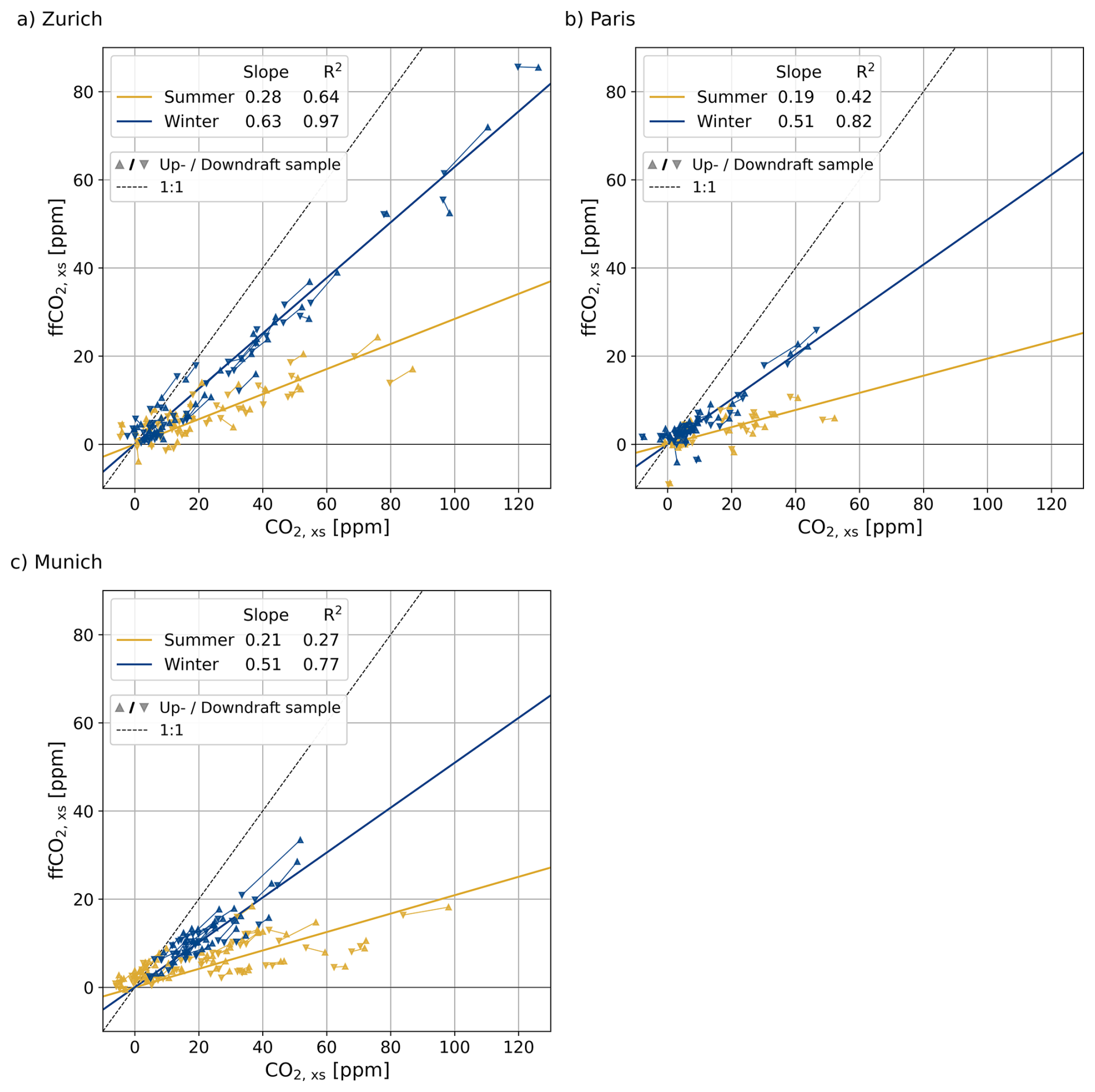
Figure 9CO2 and ffCO2 excess concentrations (“xs”) of the REA flask samples compared to concentration measurements at the European marine background station Mace Head. The pairs of updraft and downdraft measurements are connected by a line. For each site, the slope and the coefficient of determination R2 of a linear regression through the origin for the summer and winter measurements are given. For clarity, the uncertainties of about 1 ppm are omitted, but are considered in the orthogonal regression.
4.5 Comparison with regional CO2 enhancements
While the concentration differences between updraft and downdraft samples, which were used to calculate the turbulent ffCO2 fluxes (Eq. 3), were typically about 1 ppm, with a maximum of 14 ppm, the CO2 and ffCO2 enhancements compared to the background concentrations were significantly larger, especially in Zurich (median/maximum CO2 enhancement of 14/123 ppm). Moreover, the regional CO2 and ffCO2 enhancements were much more correlated than the local turbulent fluxes and showed a clear difference between summer and winter (Fig. 9). For the summer samples, the mean ffCO2 CO2 ratio obtained from orthogonal regression was 28 % for Zurich, 19 % for Paris, and 21 % for Munich, indicating that about 80 % of the net CO2 enhancements in summer were due to non-fossil CO2 emissions. For the winter samples, the average ratio was 63 % for Zurich, 51 % for Paris and 51 % for Munich, i.e., still much lower than the typical ffCO2 flux contributions in the flux footprints (compare Sect. 4.3.3).
The results illustrate that the absolute CO2 concentrations at the measurement site were primarily driven by the background concentration (between 413 and 435 ppm) and the regional CO2 fluxes integrated along the path from the marine background station to the urban area. In comparison to the local CO2 emissions, the regional fluxes were much more dominated by non-fossil CO2 emissions, in this case presumably biospheric respiration. The results agree well with those of Turnbull et al. (2015), who found that the ffCO2 enhancements measured in the city of Indianapolis with respect to a continental background station were two to three times higher than when a local background station directly upwind of the city was used. With a continental background, the ffCO2 enhancements accounted for only about 50 % of the net CO2 enhancement, whereas the local CO2 enhancement could be almost entirely explained by the ffCO2 contribution. Therefore, the CO2 fluxes analyzed in this paper represent only the local urban emissions and differ significantly from the net emissions in the surrounding area. When analyzing CO2 concentrations, the choice of the background station is of great importance and must be adapted to the scientific question.
5.1 Potentials and limitations of 14CO2 REA measurements for CO2 flux partitioning in cities (Q1)
This study demonstrates the successful implementation of the REA method for 14CO2 measurements as a powerful technique for a purely observation-based separation of fossil and non-fossil CO2 fluxes. The efficacy of the partitioning approach is demonstrated by observations of extraordinarily large nfCO2 fluxes in Munich, which could be attributed to non-fossil anthropogenic emissions from a brewery. Moreover, the Munich measurements show that with an improved technical setup and an adapted flask sampling and selection strategy, average nfCO2 fluxes of the order of 10 % or 3 µmol m−2 s−1 can be identified with a reasonable number of measurements (50 to 100). The primary contributor to the overall flux partitioning uncertainty was the current 14CO2 measurement precision in the laboratory. At the given CO2 source strengths within the flux footprints of the chosen measurement sites, the signal-to-noise ratios were often below 100 %. Situations with large fluxes are therefore favorable for the uncertainty-limited REA measurements and were preferentially selected for sample analysis. This systematic sample selection can introduce biases in the retrieved flux partitioning compared to the mean CO2 fluxes. Due to the complex, heterogeneous nature of urban environments, the micrometeorological requirements, and the costs and logistics associated with 14CO2 analyses, the 14C-based separation of ffCO2 and nfCO2 fluxes is limited to a small number of time periods and cannot be easily generalized.
5.2 Indications for large point source emissions and typical fossil and non-fossil CO2 flux compositions (Q2)
In Zurich and Munich, sectorial high ffCO2 or nfCO2 fluxes indicated significant fossil and non-fossil anthropogenic CO2 sources. Based on the respective flux footprints, these observations were potentially influenced by emissions from a district heating plant in Zurich and a brewery in Munich, respectively. Excluding the measurements potentially influenced by the identified large point-source emissions, the mean ffCO2 CO2 flux ratios of the analyzed winter measurements from the remaining urban emission mix were about 80 % to 90 % at each of the three measurement sites, with average nfCO2 fluxes of about 2 µmol m−2 s−1 in Zurich and Paris and 5 µmol m−2 s−1 in Munich. In Zurich and Paris, however, the average nfCO2 components were within the uncertainties of the partitioning approach. In Munich, on the contrary, average nfCO2 contributions were significantly larger than zero, especially in summer in the early morning and during conditions of low turbulence and/or changes in storage below the measurement height.
5.3 Compositions of local vs. regional CO2 fluxes (Q3)
While the mean ffCO2 CO2 flux ratios were about 80 % in winter and 50 % in summer, the CO2 concentration enhancements compared to marine background concentrations were in all three cities on average <63 % in winter and <28 % fossil in summer. This illustrates the locality of the urban flux footprint characterized by ffCO2 emissions compared to the significantly larger continental concentration footprint, where biogenic fluxes dominate. A thorough selection of background stations is of great importance for the interpretation of urban CO2 concentration enhancements.
Despite the limited representativity and comparatively large measurement uncertainties, the observation of substantial non-fossil CO2 fluxes underlines the necessity of separating fossil and non-fossil CO2 fluxes in cities. To maximize the number of high quality REA measurements, we recommend to clearly define the flagging criteria and research questions prior to the measurement campaign, specifying time periods, spatial directions, and micrometeorological conditions of interest. For this purpose, a near real-time metric for identifying measurements affected by storage fluxes could enable a more targeted selection or avoidance of such samples, depending on the scientific question at hand. To further increase the concentration differences between updraft and downdraft samples, and thereby the SNR, increasing the deadband width or measuring at lower heights below the inertial sublayer, closer to a particular source, could be considered. However, this would require a thorough evaluation of the statistical significance of the resulting shorter sample periods and the representativeness of the smaller footprints (see also Kunz et al., 2025a). For an independent validation of emission inventories, the REA measurements could be used for a 1:1 comparison with hourly bottom-up estimates or as input (with uncertainties) to inversion models. As shown by Stagakis et al. (2023a), the assimilation of CO2 flux observations from urban EC towers with very high spatiotemporal resolution information from urban bottom-up surface flux models has great potential for model optimization. A multi-species analysis, including MGA7 and flask measurements of co-emitted species such as CO, could allow for further attribution of emission sources and estimation of a continuous ffCO2 flux record (e.g., Maier et al., 2024b; Hilland et al., 2025; Juchem et al., 2025).
The extraordinarily large ffCO2 and nfCO2 fluxes observed from the directions of a district heating plant in Zurich and from a brewery in Munich show that to compare tall-tower measurements with bottom-up estimates or to integrate them into inversion models, inventory approaches should be able to represent large point-source emissions (both fossil and non-fossil) and their emission characteristics with high temporal resolution and three-dimensional spatial accuracy. It should also be noted that the EC method and flux footprint models rely on the assumption of stationary and horizontally homogeneous turbulent mixing. However, large point-source emissions are often associated with buoyancy fluxes and plume rise. These inhomogeneities in the turbulent mixing limit the applicability of the EC method for adequately quantifying large point-source emissions. Since emissions from large power plants and industrial facilities are generally better known than those from residential buildings, traffic, and human respiration, for example, (Super et al., 2020), it should generally be attempted to exclude atmospheric measurements affected by large point sources by analyzing wind direction, times of day, or other proxies. To this end, knowledge of the location and operating times of large emitters is essential. If the general urban mix is to be analyzed, a location without large point sources within the tower footprint should be selected, if possible.
To estimate ffCO2 concentrations, measured atmospheric Δ14C (Δ notation according to Stuiver and Polach, 1977) and CO2 concentrations are considered as the sum of a background (bg), a fossil fuel (ff), a biofuel (bf), a nuclear (nuc), a stratospheric (strato), a respiratory (resp), a photosynthetic (photo), and an oceanic (oc) component (Turnbull et al., 2016; Maier et al., 2023):
Here, Δ14C has been abbreviated by Δ14 and i = bg, ff, bf, nuc, strato, resp, photo, oc. Although not all components from Eqs. (A1) and (A2) are known, the budget equations allow, under certain assumptions, the calculation of ffCO2 differences between updraft samples and downdraft samples from REA measurements as well as between individual measurements and a background concentration. This section shows the equations and values used in this study, while detailed derivations and justifications of the assumptions can be found in the relevant literature.
A1 Concentration differences between updraft and downdraft REA samples
Combining Eqs. (A1) and (A2) and assuming that REA sample pairs differ only in their fossil fuel, non-fossil emissions (biofuel and respiration), and photosynthesis components, the difference in cff between updraft and downdraft sample can be estimated via:
We follow Maier et al. (2023) to account for the second-order effects of non-fossil 14CO2 fluxes and assume that (a) the 14CO2 signature of photosynthetic fluxes equals the mean of the updraft and downdraft flasks, (b) respiration fluxes are enriched by 25±12 ‰ compared to the mean atmospheric signature in the respective summer (July–September), and (c) that the CO2 concentration difference between updraft and downdraft flasks resulting from respiration and biofuels can be roughly accounted for with 5±5 ppm as an upper limit. Table A1 shows the assumptions and values for , , and Δcnf used for the Zurich, Paris, and Munich measurements. Details and an analysis of the corresponding uncertainties can be found in Kunz et al. (2025a).
Table A1Variables used to estimate ffCO2. denote the Δ14C values of fossil fuels (ff), photosynthetic (photo) and non-fossil emissions (nf) CO2, and flask measurements (meas). denotes the mean of the updraft and downdraft samples, which is different for each REA sampling. The atmospheric signature during CO2 uptake of the biosphere is estimated by the mean value in summer (July to September 2022/2023/2024 in the case of the Zurich/Paris/Munich campaign). Also given are the specific values derived for the measurement campaigns in each city.
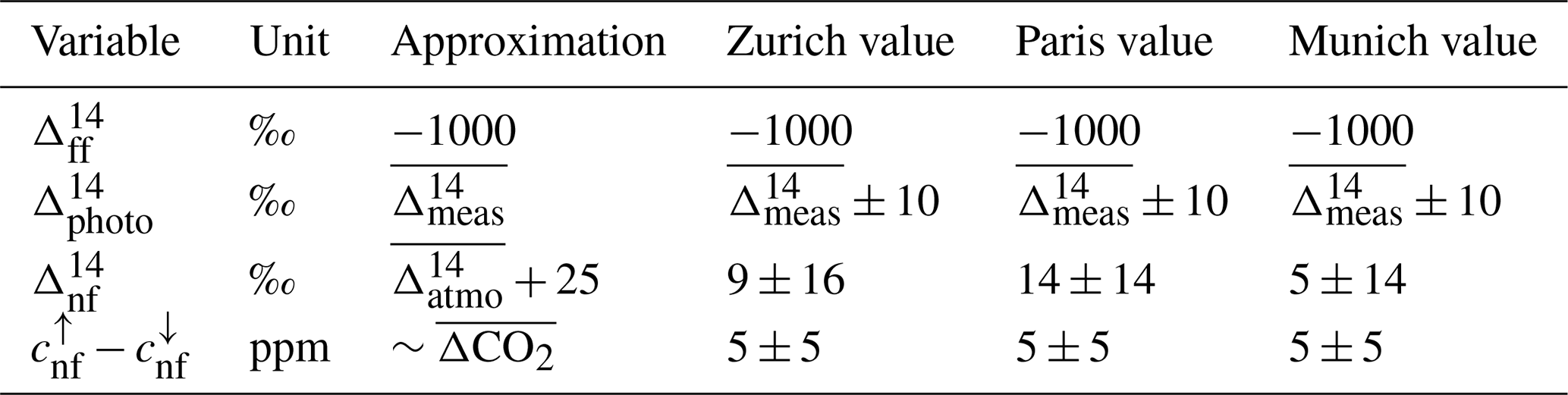
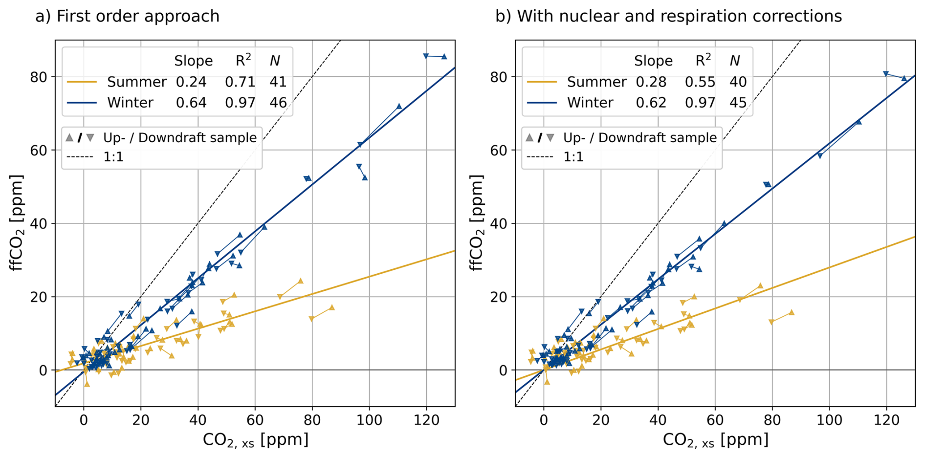
Figure A1Comparison of concentration enhancements of the Zurich REA samples with respect to MHD (a) without corrections and (b) with corrections for nuclear contamination and 14C-enriched respiration in the ffCO2 estimation. R2 is the coefficient of determination of the orthogonal regression, N the number of samples considered.
A2 Concentration differences between REA flasks and a marine background station
Approximating by , the ffCO2 concentration compared to clean background air can be calculated from Eqs. (A1) and (A2) according to Maier et al. (2023):
As described in detail in Maier et al. (2023), the background concentrations can be estimated from measurements at the ICOS station Mace Head (MHD) on the western coast of Ireland. Nuclear contributions can be modeled using a dedicated Jupyter notebook from the ICOS Carbon Portal (https://www.icos-cp.eu/data-services/tools/jupyter-notebook, last access: 20 September 2025). Respiratory concentrations can be obtained using the Vegetation Photosynthesis and Respiration Model (VPRM, Mahadevan et al., 2008) in combination with the Stochastic Time-Inverted Lagrangian Transport model (STILT, Lin et al., 2003). However, STILT simulations require meteorological input fields, which are to date only available until the end of 2023. Therefore, the nuclear and respiratory corrections (last two terms in Eq. A4) were neglected in our analysis (Levin et al., 2003). Figure A1 compares the Zurich results with and without the corrections. The slopes of the linear regressions differ about 4 %. Part of this difference is due to the exclusion of one summer and one winter sample that could have been affected by a revision of a nuclear facility. For a qualitative comparison of local ffCO2 REA fluxes and regional ffCO2 concentration enhancements, however, the nuclear and respiratory corrections are considered negligible.
B1 Stationarity and well-developed turbulence
As with any turbulent trace gas flux measurement method, stationarity and and well-developed turbulence are prerequisites for taking REA measurements (Rinne et al., 2021). We use the 0-1-2 quality control flagging scheme according to Mauder and Foken (2004), which labels “0” as high quality fluxes, “1” as medium quality fluxes, and “2” as poor quality fluxes, based on the steady state test and the developed turbulence test (Foken and Wichura, 1996). For the usually 60 min long REA measurements, the maximum of the 30 min EC averaging periods is considered.
B2 β coefficients
Figure B1 shows the CO2 flux with respect to the product of the air density ρ, the standard deviation of the vertical wind velocity σw, and the CO2 difference between updraft and downdraft flasks of all REA flask samples collected in Zurich, Paris, and Munich. The high correlation between the EC-based and the REA-based shows the high quality of both measurement methods. According to Eq. (2), the slope of a linear fit corresponds to the β coefficient. If the vertical wind velocity w were normally distributed and the regression on the CO2 concentration were linear, β would depend only on the deadband width δ. Then all data points with the same δ would fall on a line with a slope of β=0.627 for δ=0 and smaller slopes for larger δ (Grönholm et al., 2008). Deviations from this line indicate deviations from a Gaussian distribution. Since differences between individual measurements were found to be larger than differences between different scalars (Grönholm et al., 2008; Pattey et al., 1993), this is taken into account by calculating β for each sampling period individually according to Eq. (2). However, Eq. (2) is unstable for ΔCO2 close to zero, and β<0.1 or β>1 indicate non-ideal sampling conditions for REA measurements, e.g., due to skewness and kurtosis of the w time series or a linear drift leading to an unequal distribution of sampling times into the updraft and the downdraft reservoirs (Fotiadi et al., 2005a; Grönholm et al., 2008). Following Hensen et al. (2009) and Osterwalder et al. (2016), we only analyze measurements with .
Table B1β coefficients determined from the well-mixed measurements (including measurements with SNR <100 %) from a linear regression of and ΔCO2 (“Fit”, see Fig. B1) compared to the mean and standard deviation of the individually calculated β values (Eq. 2). In addition, the expected values for a normally distributed w and CO2 timeseries are given (Fotiadi et al., 2005b, no value for H=0.8 found in the literature). N denotes the number of samples considered.
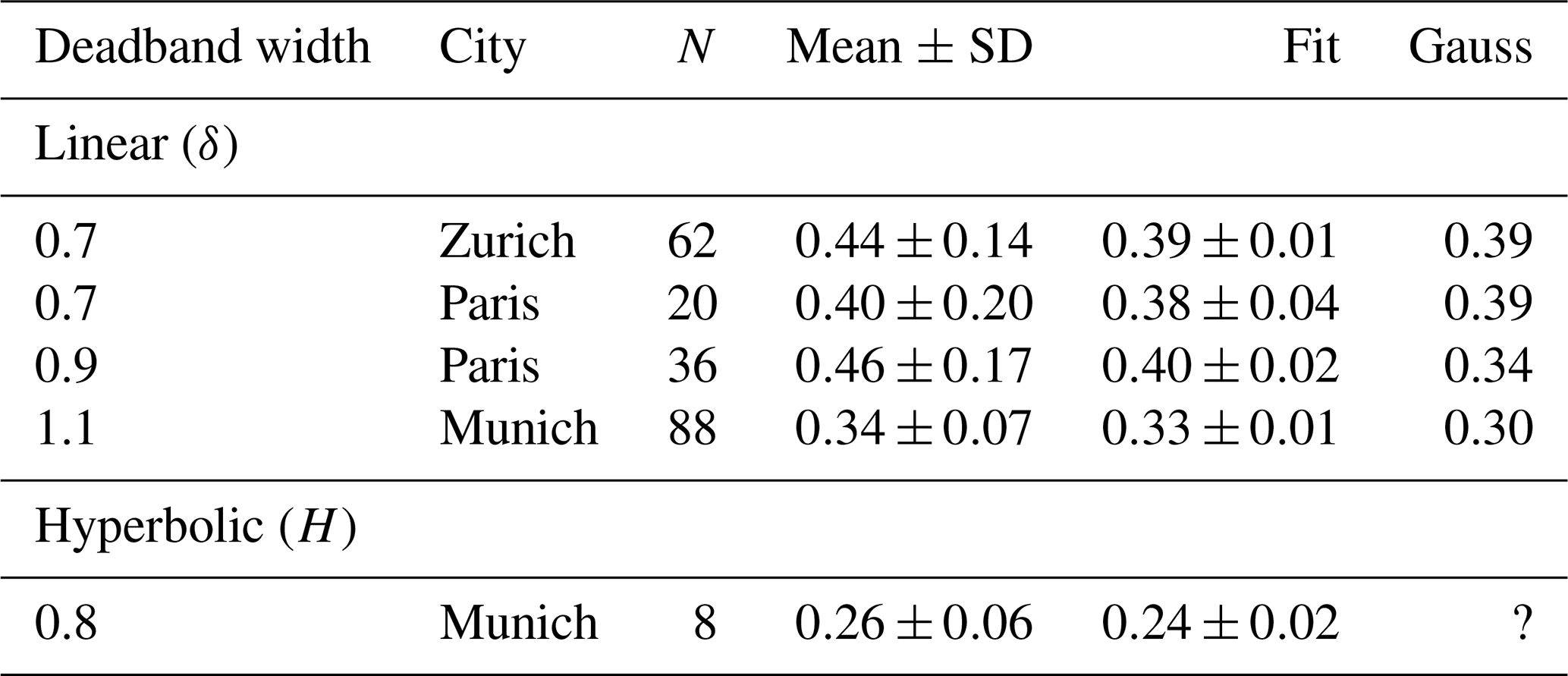
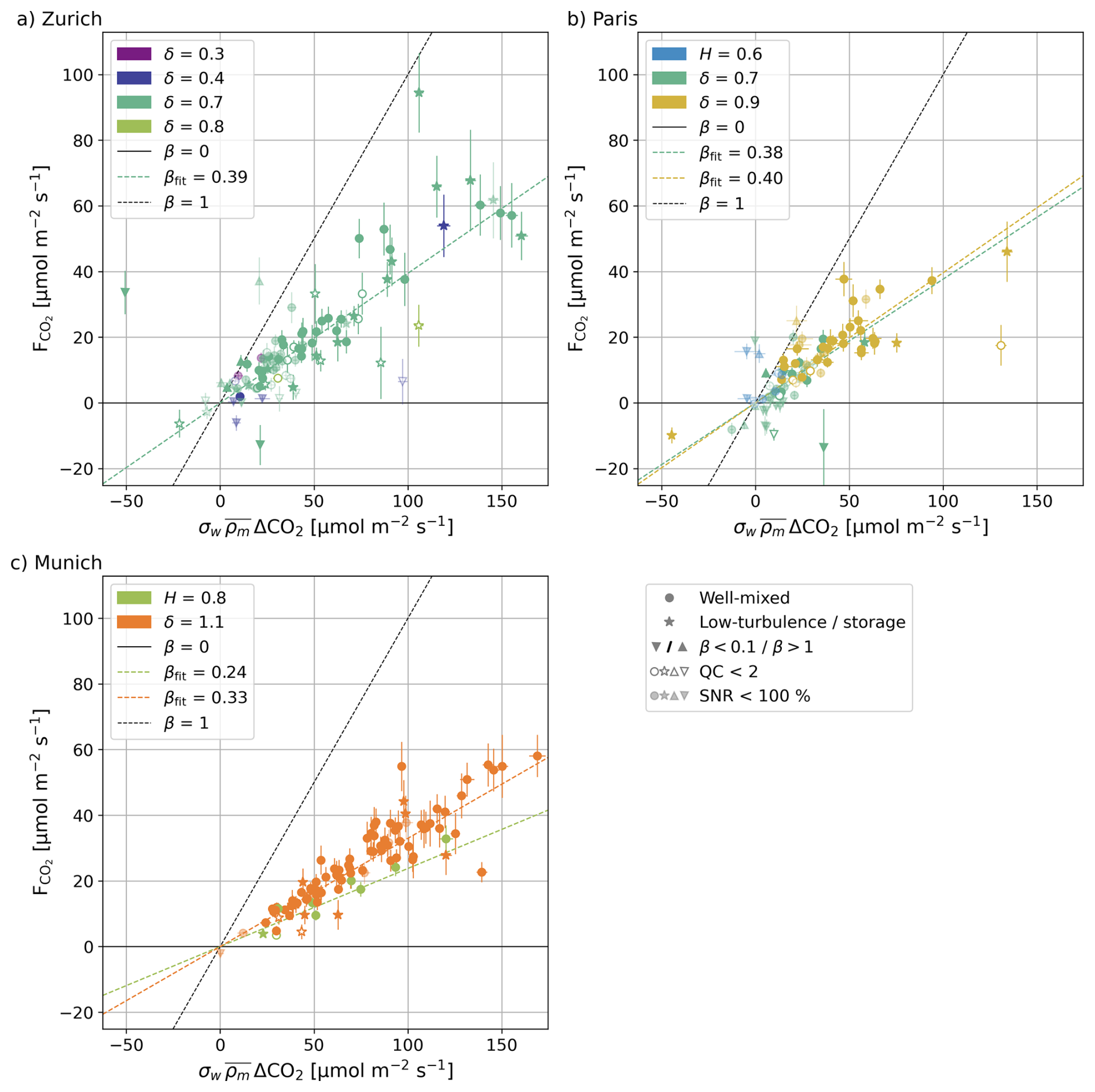
Figure B1CO2 flux vs. the standard deviation of the vertical wind velocity σw times the mean molar air density and the CO2 concentration difference between updraft and downdraft flasks of all REA flask samples collected in Zurich, Paris, and Munich. The colored dashed lines correspond to a linear regression of the well-mixed measurements (including measurements with SNR <100 %, only if N>5) with slope βfit.
B3 Signal-to-noise ratio
The calculation of fluxes based on REA measurements from Eq. (1) requires that the concentration difference between updraft and downdraft samples is greater than the measurement uncertainty. Otherwise, it is unclear whether the flux was actually small or whether it was a measurement error (Fotiadi et al., 2005a). In our case of separating net CO2 fluxes into fossil and non-fossil components, we consider the relative uncertainties of both ffCO2 and nfCO2 fluxes and discard samples only if both are >100 %, otherwise the results would be biased toward large ffCO2 fluxes. For this purpose, we define the signal-to-noise ratio (SNR) as the minimum of the relative uncertainties of the ffCO2 and the nfCO2 fluxes. Examples are shown in Fig. B2.
B4 Friction velocity and storage fluxes
During or after time periods of low turbulence, the measurement system may be decoupled from the surface so that the eddy flux is no longer representative of the local surface flux (Aubinet et al., 2012a). Instead, the measured flux will also contain non-turbulent flux components. These components can be caused by changes in storage below the measurement height or by turbulence generated at elevated layers by high wind shear, for example (low-level jets e.g., Prabha et al., 2007). The composition of these non-turbulent fluxes will be largely determined by the surface fluxes prior to the measurement period. For example, the ffCO2 CO2 ratio of a storage flux during the break up of the nocturnal boundary layer in the morning will approximately reflect the ffCO2 CO2 ratio of the integrated nocturnal CO2 emissions. Due to reduced anthropogenic emissions at night, this nocturnal ratio is assumed to be lower than the ffCO2 CO2 ratio of the surface fluxes during the measurement period (e.g., morning rush hour). Consequently, the mean ffCO2 CO2 ratio of the integrated nocturnal CO2 emissions is assumed to be smaller than the measured ffCO2 CO2 ratio. To identify the measurement periods of low turbulence and/or changes in the storage below the measurement height, we consider two quantities: the friction velocity u* and the storage flux estimated from the EC measurements.
As the assumption of well-developed turbulence for EC is often not fulfilled during periods of low friction velocity, u* is commonly used as criterion to filter EC fluxes (Aubinet et al., 2012a). Although friction velocities tend to be greater in cities due to enhanced mechanical forcing, for example, the use of a u* filter has also proved useful in many urban studies (e.g., Wu et al., 2022; Vogel et al., 2024; Hilland et al., 2025). As the continuous EC CO2 fluxes showed a systematic decrease in flux magnitude at m s−1 (Hilland et al., 2025), these periods were flagged. Since u* also becomes small during strong convective events, the u* criterion was only applied to periods with stability parameter (this threshold was chosen based on the stability range where the footprint model by Kljun et al. (2015) is applicable).
Although storage fluxes, i.e., changes in the mean CO2 concentrations within the air volume below the measurement height, are mostly negligible at higher u*, a storage flux correction is usually applied and recommended for EC flux measurements (Crawford and Christen, 2014). Since we cannot apply such a storage correction to the REA ffCO2 fluxes (see Sect. 2.2), measurements with large storage fluxes were flagged. The threshold was set to µmol m−2 s−1 (Fig. B3), which is relatively large compared to the median value of the continuous EC measurements of about 3 µmol m−2 s−1. Due to the limited number of analyzed REA samples and the large uncertainties in storage flux estimation, only the most extreme measurements were flagged. The resulting uncertainties are discussed in the text, and the results are analyzed with respect to differences between measurements taken before and after 11:00 LT (for Munich only, due to the small number of measurements in Zurich and Paris, see Sect. 4.3.3).
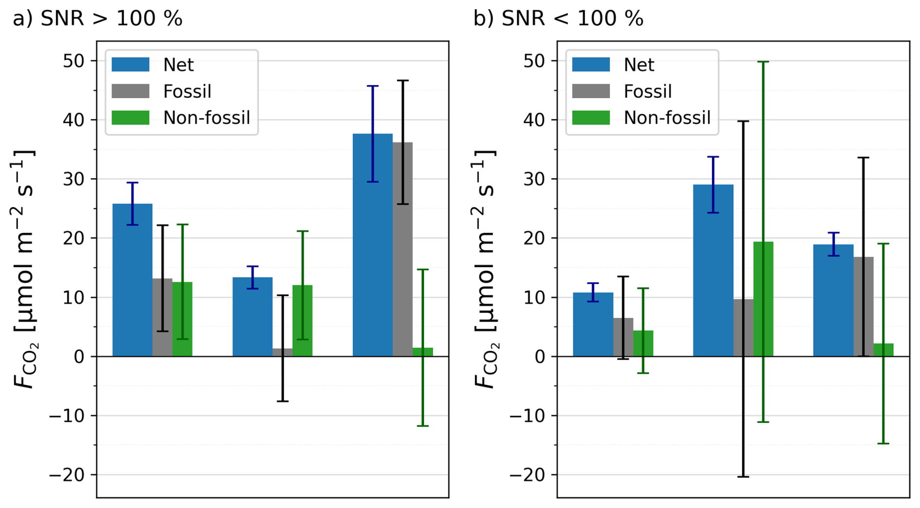
Figure B2Three examples of REA measurements with signal-to-noise ratio SNR >100 % (a) and SNR <100 % (b). SNR is defined as the minimum of the relative uncertainties of the ffCO2 and the nfCO2 fluxes.
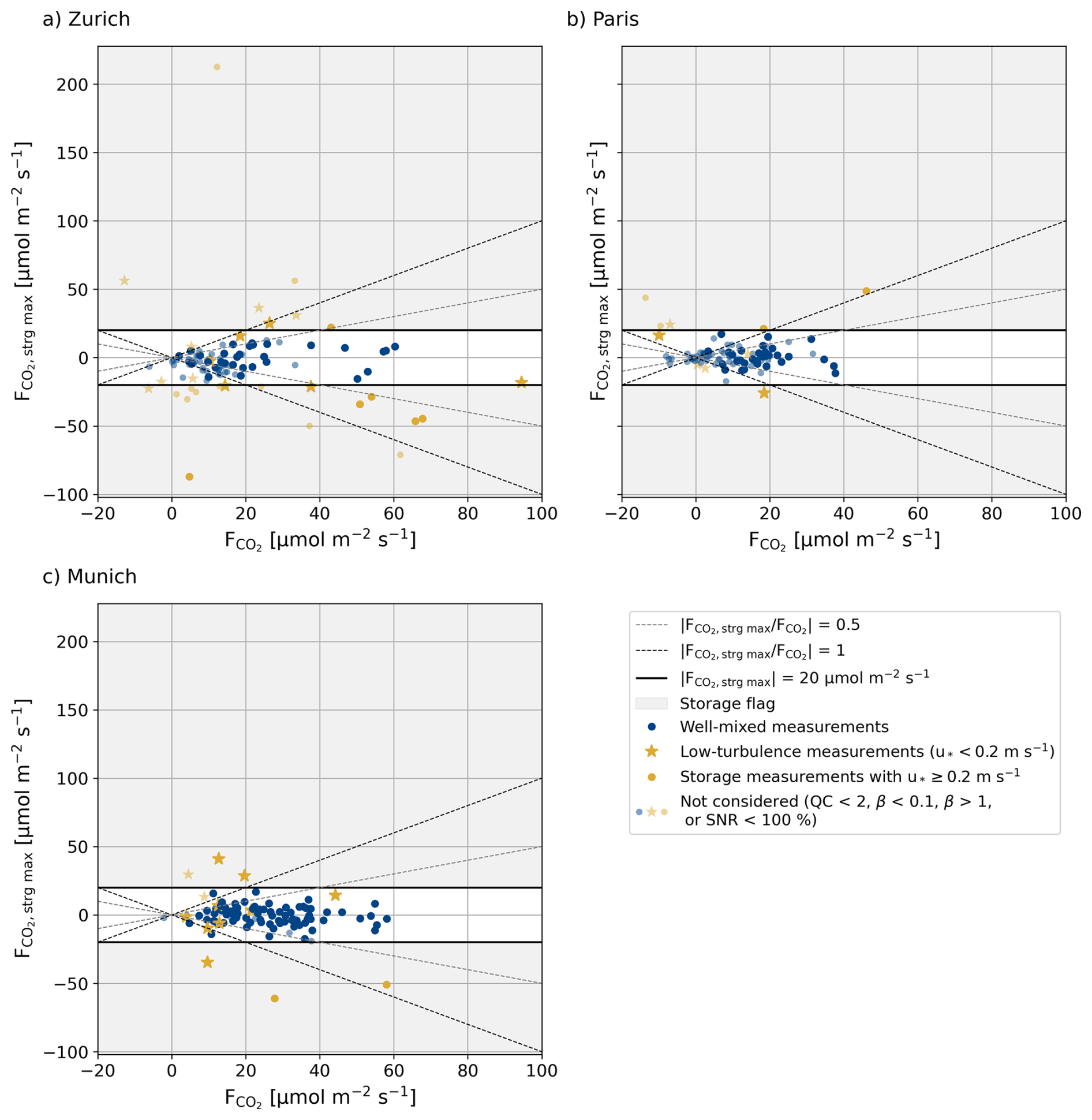
Figure B3Maximum of the 30 min storage flux estimates with respect to the mean absolute CO2 fluxes during the REA measurement periods. Measurements with µmol m−2 s−1 were flagged as storage measurements and analyzed together with the low-turbulence measurements ( m s−1).
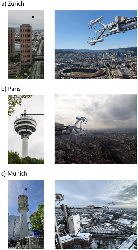
Figure C1Photos of the measurement sites in Zurich, Paris, and Munich. The black arrows indicate the height at which the IRGASON and the gas inlets (two REA inlets with fast-response valves for updrafts and downdrafts, one inlet for REA quality control tests, one inlet for MGA7 measurements) were mounted. Pictures from Roland Vogt (University of Basel), Pekka Pelkonen (ICOS RI), Pedro Henrique Herig Coimbra (INRAE), and Reiter Antennenbau-Energietechnik GmbH.
Table D1 shows the time periods covered by IRGASON measurements, used for the presentation of median net CO2 fluxes in Fig. 5. Considered were only the high and medium quality data with QC <2, m s−1, CO2 signal strength ≥90 %, and wind directions without flow distortion effects (compare Table 2). Due to later deployments and outages, the overall data coverage from MGA7 measurements is poorer. However, for most of the REA measurements, MGA7 data is available and used for the calculation of ffCO2 fluxes (Sect. 2.2).
Figure D1 shows the average normalized spectra and co-spectra of the IRGASON and the MGA7 against normalized frequency. For reference, the theoretical slopes according to Kaimal et al. (1972) are shown. In each city, the low-frequency, i.e., large energy-carrying eddies, are well captured by the MGA7. The slopes of the (co-) spectra agree well with the theoretical expectations of and , respectively. For high normalized frequencies, the impact of spectral attenuation in the intake line of the MGA7 is visible. However, these losses were corrected by applying high frequency spectral corrections according to Fratini et al. (2012). The large contribution of high frequencies observed in the IRGASON data in Paris may be related to the proximity of a strong electromagnetic source (antenna), which may be the reason for the increase the observed IRGASON noise (personal correspondence with the manufacturer). Fortunately, the IRGASON noise was not correlated to the sonic velocity, and was hence mostly filtered out by the covariance computation itself, which showed comparable and spectra. Applying high frequency corrections according to Moncrieff et al. (1997), the CO2 fluxes of the IRGASON and the MGA7 agreed well in all three cities (r2>0.89, RMSE <2.5 µmol m−2 s−1, mean bias <1.2 µmol m−2 s−1). The median time lags between the raw high-frequency CO2 measurements of the IRGASON and the MGA7 caused by clock drift and the travel time of the sample air to the MGA7 instrument (Sect. 2.1) was 4.15 s in Zurich, 10.45 s in Paris, and 37.30 s in Munich. The mean correlation between the two time lag corrected CO2 concentration time series was 0.83 in Zurich, 0.76 in Paris, and 0.83 in Munich.
Table D1Measurement periods and number (percentages) of retained measurements after quality control and filtering of the continuous CO2 flux measurements from the IRGASON instrument.
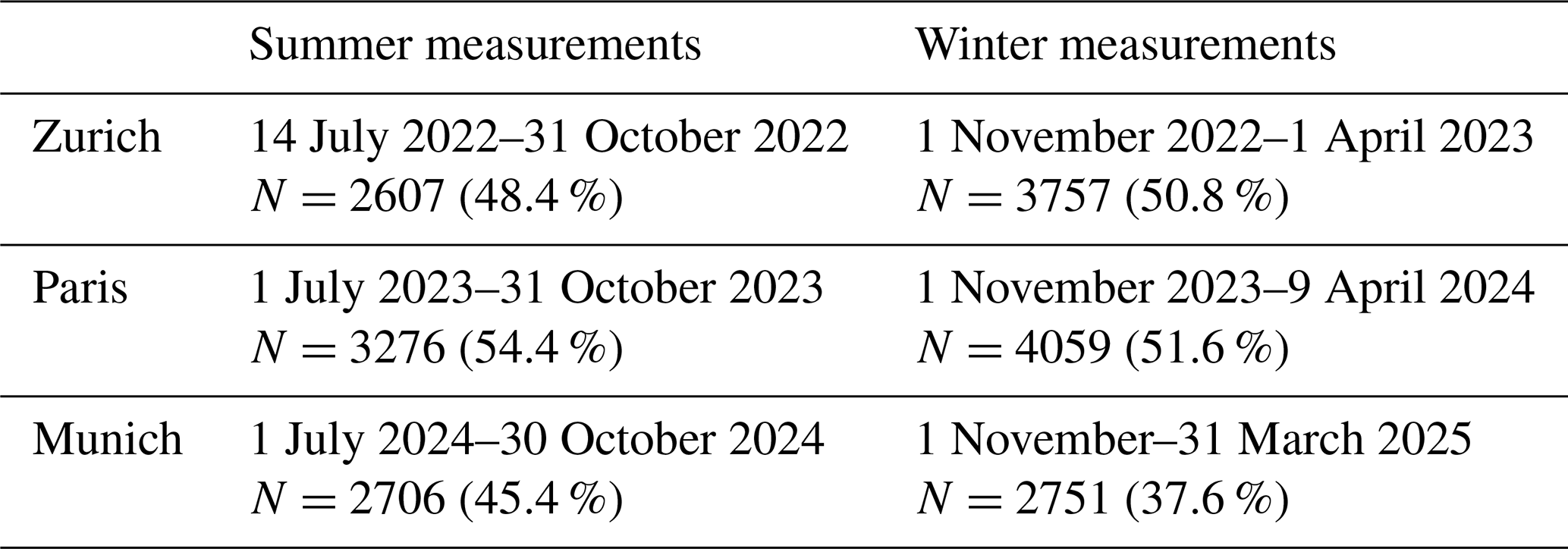
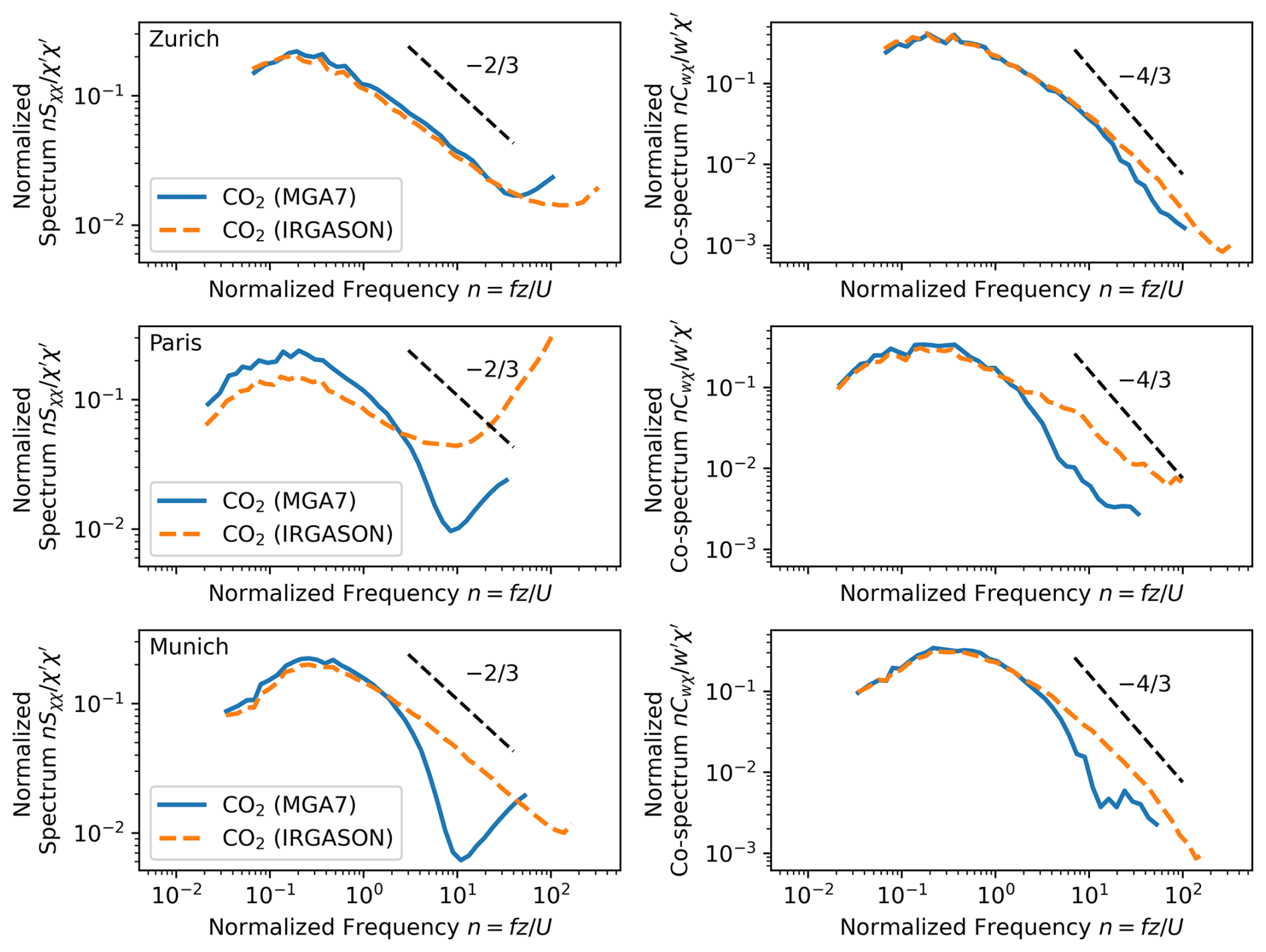
Figure D1Average normalized spectra and co-spectra against normalized frequency and theoretical slopes according to Kaimal et al. (1972).
In all three cities, quality control tests conducted approximately once a month showed an overall good agreement between the CO2 concentration of flasks sampled through the updraft and, in parallel, through the downdraft lines without switching of the valves (Table E1). The CO2 difference between these quality control flask pairs and air samples collected simultaneously through a third intake line directly into the flask sampler was slightly higher (±0.1 ppm on average). This difference can be partly attributed to the fact that with direct sampling, the weighting of the CO2 concentration over the sampling period is not completely homogeneous, leading to larger deviations if the CO2 concentration has a large variability or a trend (Levin et al., 2020; Kunz et al., 2025a). It can therefore be assumed that biases between updraft and downdraft sampling are negligible.
For the analyzed REA sample pairs, the measured CO2 differences between updraft and downdraft samples agree well with the CO2 difference estimates from both concurrent and continuous open-path IRGASON and closed-path MGA7 measurements (Table E1). As discussed in Kunz et al. (2025a), a 0.2±0.3 ppm difference between flask and IRGASON measurements in Zurich could be partly attributed to the fact that the IRGASON CO2 dry molar fractions were derived from a CO2 density output that does not properly account for high-frequency fluctuations in air temperature in the sensing path, because the ambient temperature measured by an EC100 slow-response temperature probe was used in the conversion of the absorption measurements to CO2 density. Since 13 April 2024 (end of Paris measurements), an updated logger program records the CO2 measurements using a fast-response temperature of the ultrasonic anemometer. In addition, as an open-path gas analyzer, the IRGASON is much more susceptible to weather conditions and obstructions in the path than the MGA7. The slightly smaller ΔCO2 estimates from the MGA7 in Munich may be due to high-frequency attenuation caused by the long intake lines affecting the MGA7 (100 m vs. approximately 30 m in Zurich and Paris). Nevertheless, the overall good agreement between flask and in situ measurements indicates that the system was operating as intended and that uncertainties due to the sampling process are negligible. Due to the slightly better agreement between high-precision CO2 flask measurements and the MGA7 than with the IRGASON, the MGA7 flux measurements were used when available; otherwise the fluxes calculated from the IRGASON data were used. Overall, the CO2 flux estimates from both instruments agreed well (see Appendix D). As shown in Kunz et al. (2025a) for the Zurich measurements, the ffCO2 flux uncertainties are dominated by the 14C measurement precision.
Table E1Means and standard deviations of the CO2 differences between quality control flasks sampled without switching of the valves (all-valves-open tests) through the updraft (), the downdraft () and a direct line (CO2,qc direct). Furthermore, the CO2 concentration ΔCO2 between updraft and downdraft flasks collected during the actual REA measurements are compared to estimates from the 20 Hz in situ measurements of the IRGASON and the MGA7. For the latter, only IRGASON measurements with CO2 signal strength >90 % and only MGA7 measurements with good spectral fit of the CO2 laser are considered.
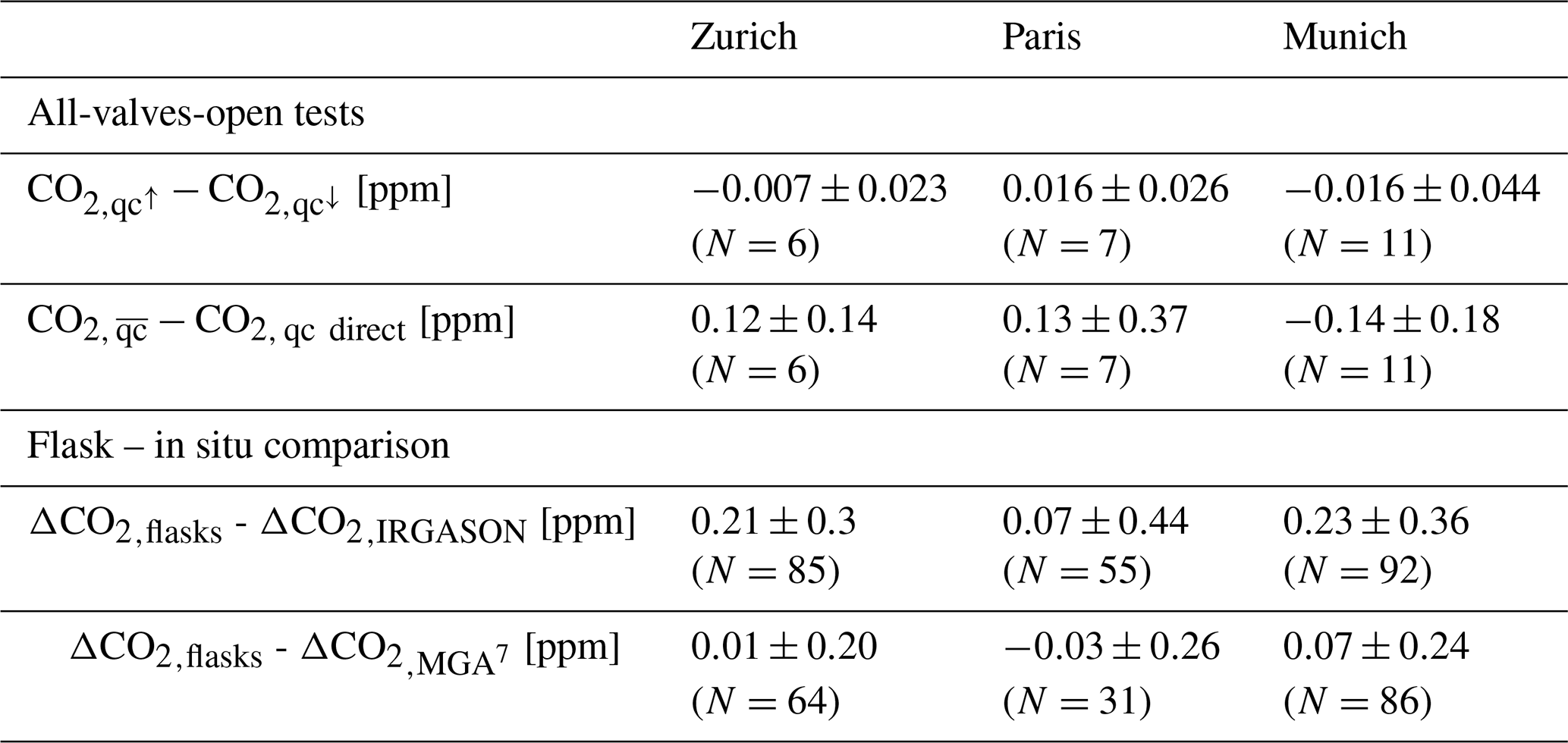
In Zurich, emissions from a district heating plant (natural gas) are likely to have influenced the REA measurements when the district heating plant was operating and within the peak area of the flux footprint (Sects. 3.1 and 4.3.2). To identify the potentially affected REA measurements, the flux contributions from a 40×40 m2 area centered around the chimney of the district heating plant were estimated based on the footprint model by Kljun et al. (2015) (Fig. F1a, left). For this purpose, two 30 min footprints were averaged for each REA measurement. There were three measurements in which the modeled footprint was in the direction of the district heating plant, but the contribution from the considered area was zero due to the finite distance of the peak contribution from the measurement site and the immediate proximity of the district heating plant to the tower (∼150 m) (Fig. F1a, right). Since the footprint model does not account for the explicit height of the point emissions (chimney of ∼ 30 m) nor plume rise due to hot emissions, and since CO2 spikes observed in the continuous concentration measurements indicate an influence from the point source, we assume that these three measurements could nevertheless have been influenced by the district heating plant. The operating times of the three burners of the district heating plant are known with a temporal resolution of 5 min.
Due to uncertainties and limitations in the footprint modeling, we also attempted to investigate the potential flux contribution from the district heating plant based on 13CO2 observations. 13C generally enables a distinction between CO2 from natural gas, which is used in the district heating plant and has a 13C signature (in δ notation) of about −40 ‰ (Tans, 1981; Widory and Javoy, 2003), and that from liquid and solid fuel or biogenic fluxes with δ13C ‰ (Tans, 1981; Widory and Javoy, 2003; Bakwin et al., 1998). However, the Zurich REA flasks were not analyzed for 13CO2 by the high-precision ICOS Flask and Calibration Laboratory, but as a by-product of the 14C extraction at the ICOS CRL, with an order of magnitude lower precision of about 0.2 ‰. Thus, although the potentially influenced samples showed influence from an isotopically lighter source, this was not significant within the measurement uncertainties, and an unambiguous gas source attribution was not possible. A contribution from a gas source is therefore likely, but cannot be clearly attributed to individual measurements. Flagging of measurements with a potential contribution from emissions from the district heating plant was therefore based on footprint data alone.
Analogously, all Munich REA measurements in which the flux footprint contribution from the area where the brewery is located was >3.5 %, were considered to be potentially influenced by emissions from the brewery (Fig. F1b). In Munich, neither the operating times nor the exact location of the emission source is known.
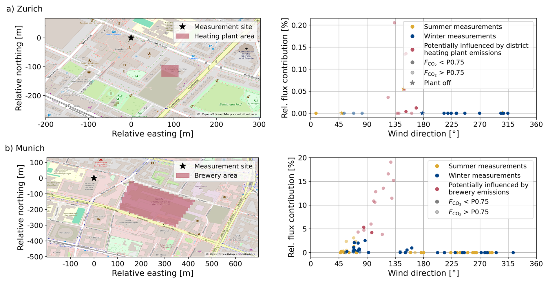
Figure F1Relative flux contributions from the areas where the district heating plant (Zurich) and the brewery (Munich) are located based on the flux footprints of the well-mixed REA measurements. Map data from © OpenStreetMap contributors 2025. Distributed under the Open Data Commons Open Database License (ODbL) v1.0, https://www.openstreetmap.org/copyright.
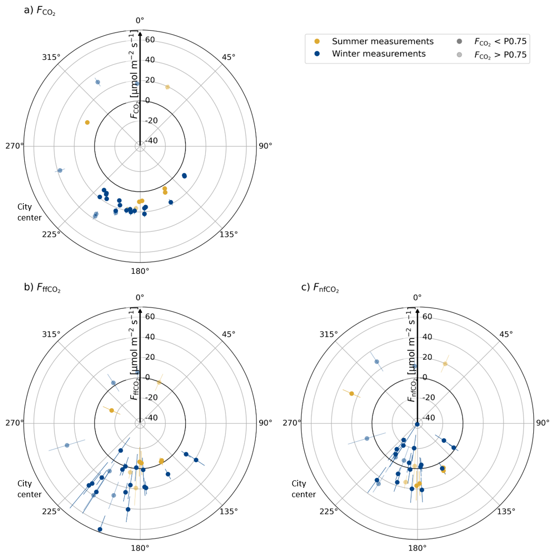
Figure G1Net CO2 fluxes (a), ffCO2 fluxes (b), and nfCO2 fluxes (c) with respect to the mean wind directions during the measurement intervals in Paris with well-mixed conditions. The error bars represent the respective flux uncertainties. P0.75 denotes the 75th percentile of the continuous EC CO2 fluxes at the respective hour of the day. Indicated is also the direction of the city center.
Since the relatively large positive and negative nfCO2 fluxes observed in Zurich and Paris for fluxes <30 µmol m−2 s−1 could not be sufficiently explained by temperature, radiation or other variables, it was investigated to what extent the results could be caused by measurement uncertainties alone and whether the available data sets show a significant difference to the naive assumption of purely fossil fluxes in the city. For this purpose, a z-test was used to calculate the probability of measuring the observed error-weighted mean ffCO2 CO2 ratios and mean nfCO2 flux under the null hypotheses of entirely fossil fluxes, i.e., % or µmol m−2 s−1, given the mean measurement uncertainties (Table 4). The null hypothesis was rejected if the p-value was less than the significance level of 0.05. Since the z-test assumes a normal distribution of the observed variables, measurements with ΔCO2 less than the measurement uncertainty of about 0.04 ppm were excluded to avoid extreme values in the ffCO2 CO2 ratio. In addition, we determined the minimum effect, i.e., the minimum deviation from the null hypothesis that would be required to correctly reject the null hypothesis at a 0.05 significance level and 80 % power. Smaller deviations from % or µmol m−2 s−1 could not be detected with the given number of samples and measurement uncertainties. The number of samples required to detect an assumed difference in the mean ffCO2 CO2 ratio of 10 % or an assumed mean nfCO2 flux of 3 µmol m−2 s−1 was also determined. Note that a constant ffCO2 CO2 ratio is not compatible with a constant nfCO2 flux. However, both are possible conceptual models that are analyzed here. Tables H1 and H2 show the results for the well-mixed measurements, divided into summer and winter measurements.
The results show that for the Paris summer measurements and for the Munich measurements the mean ffCO2 CO2 flux ratios were significantly different from 100 % (p-values <0.05), with about 20 % non-fossil contribution in winter and 50 % (Munich) and 100 % (Paris) non-fossil contribution in summer. The small fossil component in Paris is surprising and not yet fully understood. In Zurich, no significant average nfCO2 component was observed. While the small number of samples and the large measurement uncertainties in Zurich and Paris required a minimum non-fossil contribution of more than 20 % in winter and more than 40 % in summer to reject the null hypothesis/more than 300 measurements to detect a mean nfCO2 contribution of 10 % at a power of 80 %, the minimum effect was reduced to 8 % in Munich and the required number of samples to about 90 summer measurements and 50 winter measurements, respectively. Similarly, the mean nfCO2 fluxes were significantly different from zero for the Paris summer samples and the Munich samples. With the current setup, i.e., as in Munich, mean nfCO2 fluxes of 3 µmol m−2 s−1 can be determined with about 40 to 50 measurements, which is close to the number of samples collected in this study.
Table H1Analysis of the ffCO2 CO2 ratios of the well-mixed measurements, excluded those likely influenced by large point source emissions and four measurements with ΔCO2<0.4 ppm. N denotes the number of measurements, the error-weighted mean ffCO2 CO2 ratio, and the mean measurement uncertainty of the ratios. The p-values describe the probabilities of observing the measured mean ratio under the assumption (null hypothesis) that % and that deviations are solely due to measurement uncertainty. In addition, the minimum deviation from % required to reject the null hypothesis at a significance level of 0.05 (minimum effect) and the number of samples required to detect a deviation from the null hypothesis of 10 % at significance level of 0.05 and a power of 80 % (N10) is given.
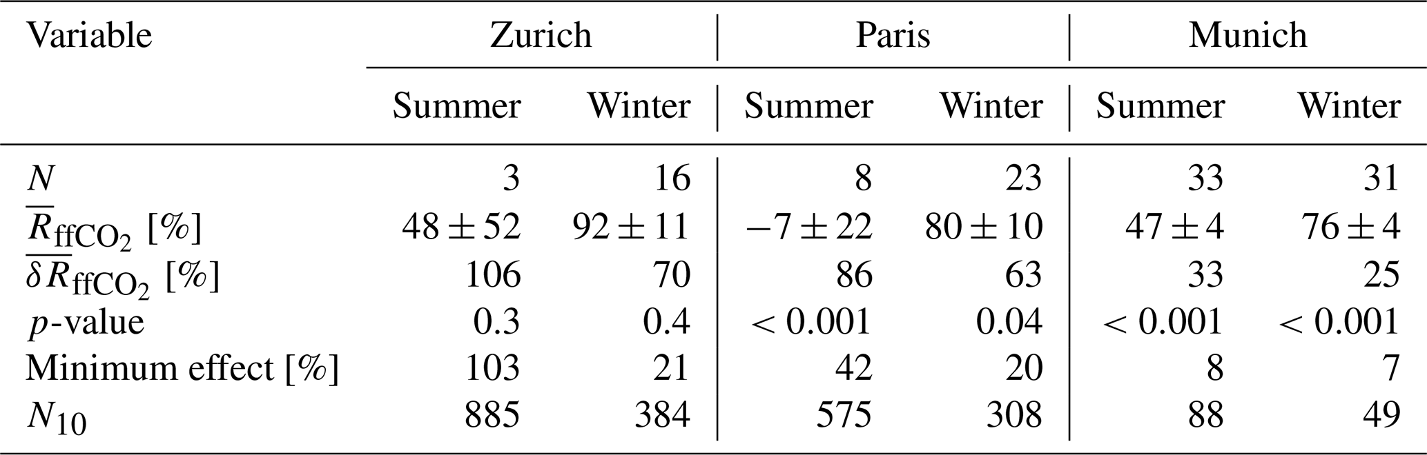
Table H2Analysis of the nfCO2 fluxes of the well-mixed measurements, excluded those likely influenced by large point source emissions and four measurements with ΔCO2<0.4 ppm. N denotes the number of measurements, the error-weighted mean nfCO2 flux, and the mean measurement uncertainty of the nfCO2 fluxes. The p-values describe the probabilities of observing the measured mean flux under the assumption (null hypothesis) that and that deviations are solely due to measurement uncertainty. In addition, the minimum deviation from required to reject the null hypothesis at a significance level of 0.05 (minimum effect) and the number of samples required to detect a deviation from the null hypothesis of 3 µmol m−2 s−1 at significance level of 0.05 and a power of 80 % (N3) is given.
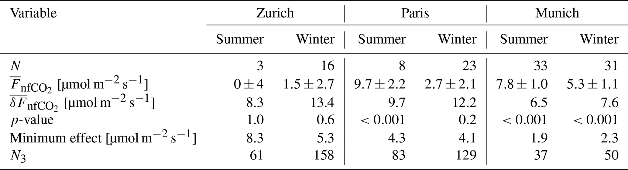
The raw data, the processed, quality-controlled fluxes, and the footprints used in this analysis are available from the ICOS Cities carbon portal https://citydata.icos-cp.eu/portal/ (last access: 1 April 2026). Flags and comments on the individual REA measurements are provided in https://doi.org/10.5281/zenodo.17183700 (Kunz et al., 2025b).
LBo, ME, RK, and VL designed and built the REA flask sampler, and helped with its installation, maintenance, and setup improvements during the three measurement campaigns. AC wrote the logger programs. AC and SH acquired funding and managed the project. LE, BL, MR, JC, CH, and MM managed the installations of the three measurement sites. SS, LBi, and CL oversaw the IRGASON measurements in Zurich, Paris, and Munich, respectively, and helped, e.g., with updates of the logger program. RH operated the MGA7 in all three cities, processed the EC data for the REA sample selection, and provided the final EC flux data used in this study. PA provided data from the midcost-sensors and helped with the installation in Munich. XG and JDC were responsible for the flask measurements at the ICOS Flask and Calibration Laboratory and the ICOS Central Radiocarbon Laboratory, AJ and SP for the corresponding data processing and quality control. BM produced the footprint and surface-cover analysis based on the model of NK. AK operated the REA system, performed the analysis, and wrote the manuscript, with conceptual and methodological input and supervision from AC, SH, and NK. All authors reviewed and contributed to the manuscript.
The contact author has declared that none of the authors has any competing interests.
Publisher's note: Copernicus Publications remains neutral with regard to jurisdictional claims made in the text, published maps, institutional affiliations, or any other geographical representation in this paper. The authors bear the ultimate responsibility for providing appropriate place names. Views expressed in the text are those of the authors and do not necessarily reflect the views of the publisher.
The authors have received funding from ICOS Cities, a.k.a. the Pilot Applications in Urban Landscapes – Towards integrated city observatories for greenhouse gases (PAUL) project, from the European Union's Horizon 2020 research and innovation program under grant agreement no. 101037319. The TUM authors are partly supported by the ERC Consolidator Grant CoSense4Climate (grant no. 101089203). Additional support was provided by internal funds and staff at the Universities of Heidelberg, Freiburg, and the Max Planck Institute for Biogeochemistry in Jena, as well as by the Swedish Strategic Research Area “ModElling the Regional and Global Earth system”, MERGE, funded by the Swedish government. Financial support from ICOS Switzerland (ICOS-CH) Phase 3 and Phase 4 (Swiss National Science Foundation, grants 20FI20_198227, 20FI-0_229655) is also acknowledged. We thank the following people for their contributions to this work: Felix Baab and Dirk Redepenning (University of Freiburg, Germany) for building the hardware at the REA inlet and logistics; Roland Vogt (University of Basel, Switzerland) and Carsten Jahn (KIT, Germany) for negotiations and installations at the Zurich and Munich sites; Pascal Rubli and Andrea Fischer (EMPA, Switzerland), Sophie Emberger (ETHZ, Switzerland), Sophie Bevini, Laura Bouillon, Ingrid Chanca, Lorna Foliot, Cécile Gaudry, and Guillaume Nief (LSCE, France), and Christian Becker and Klaus Kürzinger (TUM, Germany) for regular maintenance and logistics related to the REA flask sampler in Zurich, Paris, and Munich, respectively; Steffen Knabe and the entire staff of the ICOS Flask and Calibration Laboratory in Jena and the ICOS Central Radiocarbon Laboratory in Heidelberg for measuring the test and REA flasks; Hannes Juchem (University of Heidelberg) for providing CO2 background concentration data from Mace Head; Matthias Zeeman (University of Freiburg, Germany) for managing the data infrastructure. We would also like to thank Kenneth Davis and the anonymous reviewer for their comments and suggestions, which helped to improve the paper. DeepL was used for grammar and spell checking.
This research has been supported by the EU Horizon 2020 (grant no. 101037319).
This open-access publication was funded by the University of Freiburg.
This paper was edited by Thomas Karl and reviewed by Kenneth Davis and one anonymous referee.
Aigner, P., Chen, J., Böhm, F., Chariot, M., Emmenegger, L., Frölich, L., Grange, S., Kühbacher, D., Kürzinger, K., Laurent, O., Makowski, M., Rubli, P., Schmitt, A., and Wenzel, A.: ACROPOLIS: Munich urban CO2 sensor network, Atmos. Meas. Tech., 19, 745–773, https://doi.org/10.5194/amt-19-745-2026, 2026. a
Aubinet, M., Feigenwinter, C., Heinesch, B., Laffineur, Q., Papale, D., Reichstein, M., Rinne, J., and van Gorsel, E.: Nighttime Flux Correction, in: Eddy Covariance, edited by: Aubinet, M., Vesala, T., and Papale, D., Springer, Dordrecht, 133–158, https://doi.org/10.1007/978-94-007-2351-1_5, 2012a. a, b
Aubinet, M., Vesala, T., and Papale, D. (Eds.): Eddy Covariance, Springer, Dordrecht, https://doi.org/10.1007/978-94-007-2351-1, 2012b. a, b
Bakwin, P. S., Tans, P. P., White, J. W. C., and Andres, R. J.: Determination of the isotopic (13C/12C) discrimination by terrestrial biology from a global network of observations, Global Biogeochem. Cy., 12, 555–562, https://doi.org/10.1029/98GB02265, 1998. a
Bowling, D. R., Delany, A. C., Turnipseed, A. A., Baldocchi, D. D., and Monson, R. K.: Modification of the relaxed eddy accumulation technique to maximize measured scalar mixing ratio differences in updrafts and downdrafts, J. Geophys. Res., 104, 9121–9133, https://doi.org/10.1029/1999JD900013, 1999. a
Crawford, B. and Christen, A.: Spatial variability of carbon dioxide in the urban canopy layer and implications for flux measurements, Atmos. Environ., 98, 308–322, https://doi.org/10.1016/j.atmosenv.2014.08.052, 2014. a, b, c, d
Crawford, B. and Christen, A.: Spatial source attribution of measured urban eddy covariance CO2 fluxes, Theor. Appl. Climatol., 119, 733–755, https://doi.org/10.1007/s00704-014-1124-0, 2015. a
Dröge, R., Denier van der Gon, H., Perrussel, O., David, L., Aigner, P., Kuehbacher, D., Chen, J., Hinderer, J., Brunner, D., and Constantin, L.: Final version of high-resolution city emission inventory for GHGs and co-emitted species for 2018, 2020 and 2022, ICOS ERIC – Carbon Portal, https://doi.org/10.18160/0GEF-R5XX, 2024. a
Ecosystem Thematic Centre: ETC NRT Fluxes from Oberpostdirektion, 2023-01-05–2025-05-25, ICOS Cities, https://hdl.handle.net/11676/CTRT8e-iMrXMpADFNC87AVlp, 2025. a
Elshani, A., Pehlivani, K., Kelmendi, B., and Cacaj, I.: Possibility and determination of the use of CO2 produced by the production of beers, Journal of Pharmaceutical Sciences and Research, 10, 1229–1230, 2018. a
Finkelstein, P. L. and Sims, P. F.: Sampling error in eddy correlation flux measurements, J. Geophys. Res., 106, 3503–3509, https://doi.org/10.1029/2000JD900731, 2001. a
Foken, T. and Wichura, B.: Tools for quality assessment of surface-based flux measurements, Agr. Forest Meteorol., 78, 83–105, https://doi.org/10.1016/0168-1923(95)02248-1, 1996. a
Fotiadi, A., Lohou, F., Druilhet, A., Serça, D., Saïd, F., Laville, P., and Brut, A.: Methodological Development of the Conditional Sampling Method. Part II: Quality Control Criteria of Relaxed Eddy Accumulation Flux Measurements, Bound.-Lay. Meteorol., 117, 577–603, https://doi.org/10.1007/s10546-005-4497-x, 2005a. a, b, c, d
Fotiadi, A. K., Lohou, F., Druilhet, A., Sera, D., Brunet, Y., and Delmas, R.: Methodological Development of the Conditional Sampling Method. Part I: Sensitivity to Statistical and Technical Characteristics, Bound.-Lay. Meteorol., 114, 615–640, https://doi.org/10.1007/s10546-004-1080-9, 2005b. a, b, c
Fratini, G., Ibrom, A., Arriga, N., Burba, G., and Papale, D.: Relative humidity effects on water vapour fluxes measured with closed-path eddy-covariance systems with short sampling lines, Agr. Forest Meteorol., 165, 53–63, https://doi.org/10.1016/j.agrformet.2012.05.018, 2012. a, b
Grönholm, T., Haapanala, S., Launiainen, S., Rinne, J., Vesala, T., and Rannik, U.: The dependence of the beta coefficient of REA system with dynamic deadband on atmospheric conditions, Environ. Pollut., 152, 597–603, https://doi.org/10.1016/j.envpol.2007.06.071, 2008. a, b, c, d
Hensen, A., Nemitz, E., Flynn, M. J., Blatter, A., Jones, S. K., Sørensen, L. L., Hensen, B., Pryor, S. C., Jensen, B., Otjes, R. P., Cobussen, J., Loubet, B., Erisman, J. W., Gallagher, M. W., Neftel, A., and Sutton, M. A.: Inter-comparison of ammonia fluxes obtained using the Relaxed Eddy Accumulation technique, Biogeosciences, 6, 2575–2588, https://doi.org/10.5194/bg-6-2575-2009, 2009. a, b, c
Hersbach, H., Bell, B., Berrisford, P., Biavati, G., Horányi, A., Muñoz Sabater, J., Nicolas, J., Peubey, C., Radu, R., Rozum, I., Schepers, D., Simmons, A., Soci, C., Dee, D., and Thépaut, J.-N.: ERA5 hourly data on single levels from 1940 to present, Copernicus Climate Change Service (C3S) Climate Data Store (CDS), https://doi.org/10.24381/cds.adbb2d47, 2024. a
Hilland, R., Hashemi, J., Stagakis, S., Brunner, D., Constantin, L., Kljun, N., Kunz, A.-K., Molinier, B., Hammer, S., Emmenegger, L., and Christen, A.: Sectoral attribution of greenhouse gas and pollutant emissions using multi-species eddy covariance on a tall tower in Zurich, Switzerland, Atmos. Chem. Phys., 25, 14279–14299, https://doi.org/10.5194/acp-25-14279-2025, 2025. a, b, c, d, e, f, g, h
ICOS Ecosystem Thematic Centre, Bignotti, L., Loubet, B., Depuydt, J., Buysse, P., Coimbra, P., Fortineau, A., Nief, G., Ramonet, M., Stagakis, S., Christen, A., Hilland, R., and Nicolini, G.: ETC L2 Fluxes from Romainville, 2022-12-31–2024-12-31, ICOS Cities, https://hdl.handle.net/11676/TwGCXiTNxEpW-Iq_r8esdE5v, 2025a. a
ICOS Ecosystem Thematic Centre, Holst, C., Lan, C., Jahn, C., Christen, A., Hilland, R., Stagakis, S., and Nicolini, G., Mauder, M.: ETC L2 Fluxes from Oberpostdirektion, 2022-12-31–2024-12-31, ICOS Cities, https://hdl.handle.net/11676/WNOldo0yJzYBwDyrywI3oQaX, 2025b. a
ICOS Ecosystem Thematic Centre, Stagakis, S., Vogt, R., Christen, A., Hilland, R., and Nicolini, G.: ETC L2 Fluxes from Hardau, 2021-12-31–2024-12-31, ICOS Cities, https://hdl.handle.net/11676/Lg2RRHAdsLee0lsF-9KsTC-r, 2025c. a
Juchem, H., Maier, F., Levin, I., Jordan, A., Pöhler, D., Rosendahl, C., Della Coletta, J., Preunkert, S., and Hammer, S.: Challenges and benefits of using NOx as a quantitative proxy for fossil fuel CO2 in an urban area based on radiocarbon measurements, Atmos. Chem. Phys., 25, 18373–18388, https://doi.org/10.5194/acp-25-18373-2025, 2025. a
Kaimal, J. C., Wyngaard, J. C., Izumi, Y., and Coté, O. R.: Spectral characteristics of surface–layer turbulence, Q. J. Roy. Meteor. Soc., 98, 563–589, https://doi.org/10.1002/qj.49709841707, 1972. a, b
Kellett, R., Christen, A., Coops, N. C., van der Laan, M., Crawford, B., Tooke, T. R., and Olchovski, I.: A systems approach to carbon cycling and emissions modeling at an urban neighborhood scale, Landscape Urban Plan., 110, 48–58, https://doi.org/10.1016/j.landurbplan.2012.10.002, 2013. a
Kljun, N., Calanca, P., Rotach, M. W., and Schmid, H. P.: A simple two-dimensional parameterisation for Flux Footprint Prediction (FFP), Geosci. Model Dev., 8, 3695–3713, https://doi.org/10.5194/gmd-8-3695-2015, 2015. a, b, c, d, e
Kunz, A.-K., Borchardt, L., Christen, A., Della Coletta, J., Eritt, M., Gutiérrez, X., Hashemi, J., Hilland, R., Jordan, A., Kneißl, R., Legendre, V., Levin, I., Preunkert, S., Rubli, P., Stagakis, S., and Hammer, S.: Flask data and logger program supporting the manuscript ”A relaxed eddy accumulation flask sampling system for 14C-based partitioning of fossil and non-fossil CO2 fluxes” (v1.0.0-pre), Zenodo, https://doi.org/10.5281/zenodo.13926681, 2024. a
Kunz, A.-K., Borchardt, L., Christen, A., Della Coletta, J., Eritt, M., Gutiérrez, X., Hashemi, J., Hilland, R., Jordan, A., Kneißl, R., Legendre, V., Levin, I., Preunkert, S., Rubli, P., Stagakis, S., and Hammer, S.: A relaxed eddy accumulation flask sampling system for 14C-based partitioning of fossil and non-fossil CO2 fluxes, Atmos. Meas. Tech., 18, 5349–5373, https://doi.org/10.5194/amt-18-5349-2025, 2025a. a, b, c, d, e, f, g, h, i, j, k, l, m, n, o, p, q
Kunz, A.-K., Hammer, S., Aigner, P., Bignotti, L., Borchardt, L., Chen, J., Della Coletta, J., Emmenegger, L., Eritt, M., Gutiérrez, X., Hashemi, J., Hilland, R., Holst, C. C., Jordan, A., Kljun, N., Kneißl, R., Lan, C., Legendre, V., Levin, I., Loubet, B., Mauder, M., Molinier, B., Preunkert, S., Ramonet, M., Stagakis, S., and Christen, A.: Data supporting the manuscript “14C-based separation of fossil and non-fossil CO2 fluxes in cities using relaxed eddy accumulation: results from tall-tower measurements in Zurich, Paris, and Munich”, https://doi.org/10.5281/zenodo.17183700, Zenodo [data set], 2025b. a, b, c
Lan, C., Mauder, M., Stagakis, S., Loubet, B., D'Onofrio, C., Metzger, S., Durden, D., and Herig-Coimbra, P.-H.: Intercomparison of eddy-covariance software for urban tall-tower sites, Atmos. Meas. Tech., 17, 2649–2669, https://doi.org/10.5194/amt-17-2649-2024, 2024. a
Lan, L., Ghasemifard, H., Yuan, Y., Hachinger, S., Zhao, X., Bhattacharjee, S., Bi, X., Bai, Y., Menzel, A., and Chen, J.: Assessment of Urban CO2 Measurement and Source Attribution in Munich Based on TDLAS-WMS and Trajectory Analysis, Atmosphere, 11, 58, https://doi.org/10.3390/atmos11010058, 2020. a
Levin, I., Kromer, B., Schmidt, M., and Sartorius, H.: A novel approach for independent budgeting of fossil fuel CO2 over Europe by 14CO2 observations, Geophys. Res. Lett., 30, https://doi.org/10.1029/2003GL018477, 2003. a, b, c, d, e
Levin, I., Karstens, U., Eritt, M., Maier, F., Arnold, S., Rzesanke, D., Hammer, S., Ramonet, M., Vítková, G., Conil, S., Heliasz, M., Kubistin, D., and Lindauer, M.: A dedicated flask sampling strategy developed for Integrated Carbon Observation System (ICOS) stations based on CO2 and CO measurements and Stochastic Time-Inverted Lagrangian Transport (STILT) footprint modelling, Atmos. Chem. Phys., 20, 11161–11180, https://doi.org/10.5194/acp-20-11161-2020, 2020. a
LI-COR: EddyPro Software version 7.0: Instruction Manual, https://www.licor.com/env/support/EddyPro/manuals.html (last access: 5 October 2025), 2021. a
Lin, J. C., Gerbig, C., Wofsy, S. C., Andrews, A. E., Daube, B. C., Davis, K. J., and Grainger, C. A.: A near–field tool for simulating the upstream influence of atmospheric observations: The Stochastic Time–Inverted Lagrangian Transport (STILT) model, J. Geophys. Res., 108, https://doi.org/10.1029/2002JD003161, 2003. a
Mahadevan, P., Wofsy, S. C., Matross, D. M., Xiao, X., Dunn, A. L., Lin, J. C., Gerbig, C., Munger, J. W., Chow, V. Y., and Gottlieb, E. W.: A satellite–based biosphere parameterization for net ecosystem CO2 exchange: Vegetation Photosynthesis and Respiration Model (VPRM), Global Biogeochem. Cy., 22, https://doi.org/10.1029/2006GB002735, 2008. a
Maier, F., Levin, I., Gachkivskyi, M., Rödenbeck, C., and Hammer, S.: Estimating regional fossil fuel CO2 concentrations from 14CO2 observations: challenges and uncertainties, Philos. T. R. Soc. A, 381, 20220203, https://doi.org/10.1098/rsta.2022.0203, 2023. a, b, c, d, e, f
Maier, F., Levin, I., Conil, S., Gachkivskyi, M., Denier van der Gon, H., and Hammer, S.: Uncertainty in continuous ΔCO-based ΔffCO2 estimates derived from 14C flask and bottom-up ΔCO / ΔffCO2 ratios, Atmos. Chem. Phys., 24, 8205–8223, https://doi.org/10.5194/acp-24-8205-2024, 2024. 2024a. a, b
Maier, F., Rödenbeck, C., Levin, I., Gerbig, C., Gachkivskyi, M., and Hammer, S.: Potential of 14C-based vs. ΔCO-based ΔffCO2 observations to estimate urban fossil fuel CO2 (ffCO2) emissions, Atmos. Chem. Phys., 24, 8183–8203, https://doi.org/10.5194/acp-24-8183-2024, 2024b. a, b
Mauder, M. and Foken, T.: Documentation and instruction manual of the eddy-covariance software package TK2, Arbeitsergebnisse, Universität Bayreuth, Abt. Mikrometeorologie, 26, ISSN 1614-8924, 2004. a, b, c
Mauder, M., Cuntz, M., Drüe, C., Graf, A., Rebmann, C., Schmid, H. P., Schmidt, M., and Steinbrecher, R.: A strategy for quality and uncertainty assessment of long-term eddy-covariance measurements, Agr. Forest Meteorol., 169, 122–135, https://doi.org/10.1016/j.agrformet.2012.09.006, 2013. a, b
Miller, J. B., Lehman, S. J., Verhulst, K. R., Miller, C. E., Duren, R. M., Yadav, V., Newman, S., and Sloop, C. D.: Large and seasonally varying biospheric CO2 fluxes in the Los Angeles megacity revealed by atmospheric radiocarbon, P. Natl. Acad. Sci. USA, 117, 26681–26687, https://doi.org/10.1073/pnas.2005253117, 2020. a, b, c
Milne, R., Beverland, I. J., Hargreaves, K., and Moncrieff, J. B.: Variation of the β coefficient in the relaxed eddy accumulation method, Bound.-Lay. Meteorol., 93, 211–225, https://doi.org/10.1023/A:1002061514948, 1999. a
Molinier, B. and Kljun, N.: Footprints for the flux towers in three pilot cities: Deliverable 2.6. Project number 101037319, https://icos-ri.atlassian.net/wiki/spaces/PP/pages/10518555/Deliverables (last access: 11 January 2026), 2024. a
Moncrieff, J., Clement, R., Finnigan, J., and Meyers, T.: Averaging, Detrending, and Filtering of Eddy Covariance Time Series, in: Handbook of Micrometeorology, edited by: Lee, X., Massman, W., and Law, B., Atmospheric and Oceanographic Sciences Library, Springer, Dordrecht, 7–31, https://doi.org/10.1007/1-4020-2265-4_2, 2004. a
Moncrieff, J. B., Massheder, J. M., de Bruin, H., Elbers, J., Friborg, T., Heusinkveld, B., Kabat, P., Scott, S., Soegaard, H., and Verhoef, A.: A system to measure surface fluxes of momentum, sensible heat, water vapour and carbon dioxide, J. Hydrol., 188–189, 589–611, https://doi.org/10.1016/S0022-1694(96)03194-0, 1997. a, b
Moriwaki, R., Kanda, M., and Nitta, H.: Carbon dioxide build-up within a suburban canopy layer in winter night, Atmos. Environ., 40, 1394–1407, https://doi.org/10.1016/j.atmosenv.2005.10.059, 2006. a
Olajire, A. A.: The brewing industry and environmental challenges, J. Clean. Prod., 256, 102817, https://doi.org/10.1016/j.jclepro.2012.03.003, 2020. a
Osterwalder, S., Fritsche, J., Alewell, C., Schmutz, M., Nilsson, M. B., Jocher, G., Sommar, J., Rinne, J., and Bishop, K.: A dual-inlet, single detector relaxed eddy accumulation system for long-term measurement of mercury flux, Atmos. Meas. Tech., 9, 509–524, https://doi.org/10.5194/amt-9-509-2016, 2016. a, b, c
Pattey, E., Desjardins, R. L., and Rochette, P.: Accuracy of the relaxed eddy-accumulation technique, evaluated using CO2 flux measurements, Bound.-Lay. Meteorol., 66, 341–355, https://doi.org/10.1007/BF00712728, 1993. a, b, c, d
Prabha, T. V., Leclerc, M. Y., Karipot, A., and Hollinger, D. Y.: Low-Frequency Effects on Eddy Covariance Fluxes under the Influence of a Low-Level Jet, J. Appl. Meteorol. Clim., 46, 338–352, https://doi.org/10.1175/JAM2461.1, 2007. a
Rebmann, C., Kolle, O., Heinesch, B., Queck, R., Ibrom, A., and Aubinet, M.: Data Acquisition and Flux Calculations, in: Eddy Covariance, edited by: Aubinet, M., Vesala, T., and Papale, D., Springer, Dordrecht, 59–84, https://doi.org/10.1007/978-94-007-2351-1_3, 2012. a
Rinne, J., Ammann, C., Pattey, E., Paw U, K. T., and Desjardins, R. L.: Alternative Turbulent Trace Gas Flux Measurement Methods, in: Springer Handbook of Atmospheric Measurements, edited by: Foken, T., Springer Handbooks, Springer, Cham, 1505–1530, https://doi.org/10.1007/978-3-030-52171-4_56, 2021. a, b, c
Stagakis, S., Feigenwinter, C., Vogt, R., Brunner, D., and Kalberer, M.: A high-resolution monitoring approach of urban CO2 fluxes. Part 2 – surface flux optimisation using eddy covariance observations, Sci. Total Environ., 903, 166035, https://doi.org/10.1016/j.scitotenv.2023.166035, 2023a. a
Stagakis, S., Feigenwinter, C., Vogt, R., and Kalberer, M.: A high-resolution monitoring approach of urban CO2 fluxes. Part 1 – bottom-up model development, Sci. Total Environ., 858, 160216, https://doi.org/10.1016/j.scitotenv.2022.160216, 2023b. a
Stagakis, S., Brunner, D., Li, J., Backman, L., Karvonen, A., Constantin, L., Järvi, L., Havu, M., Chen, J., Emberger, S., and Kulmala, L.: Intercomparison of biogenic CO2 flux models in four urban parks in the city of Zurich, Biogeosciences, 22, 2133–2161, https://doi.org/10.5194/bg-22-2133-2025, 2025. a, b, c, d
Stuiver, M. and Polach, H. A.: Discussion Reporting of 14C Data, Radiocarbon, 19, 355–363, https://doi.org/10.1017/S0033822200003672, 1977. a, b
Stull, R. B.: An Introduction to Boundary Layer Meteorology, vol. 13 of Atmospheric and Oceanographic Sciences Library, Springer, Dordrecht, https://doi.org/10.1007/978-94-009-3027-8, 1988. a, b
Super, I., Dellaert, S. N. C., Visschedijk, A. J. H., and Denier van der Gon, H. A. C.: Uncertainty analysis of a European high-resolution emission inventory of CO2 and CO to support inverse modelling and network design, Atmos. Chem. Phys., 20, 1795–1816, https://doi.org/10.5194/acp-20-1795-2020, 2020. a
Tans, P. and Zellweger, C. (Eds.): GAW Report No. 213, 17th WMO/IAEA Meeting on carbon dioxide, other greenhouse gases and related tracers measurement techniques (GGMT-2013), Beijing, China, 10–13 June 2013, https://www.uncclearn.org/wp-content/uploads/library/gaw_213_en.pdf (last access: 5 October 2025), 2014. a
Tans, P. P.: 13C/12C of industrial CO2, Carbon Cycle Modelling, 16, 127–129, 1981. a, b
Turnbull, J. C., Sweeney, C., Karion, A., Newberger, T., Lehman, S. J., Tans, P. P., Davis, K. J., Lauvaux, T., Miles, N. L., Richardson, S. J., Cambaliza, M. O., Shepson, P. B., Gurney, K., Patarasuk, R., and Razlivanov, I.: Toward quantification and source sector identification of fossil fuel CO2 emissions from an urban area: Results from the INFLUX experiment, J. Geophys. Res., 120, 292–312, https://doi.org/10.1002/2014JD022555, 2015. a, b, c, d
Turnbull, J. C., Graven, H., and Krakauer, N. Y.: Radiocarbon in the Atmosphere, in: Radiocarbon and Climate Change, edited by: Schuur, E. A., Druffel, E. R. M., and Trumbore, S. E., Springer, Cham, 83–137, https://doi.org/10.1007/978-3-319-25643-6_4, 2016. a
Vogel, E., Davis, K. J., Wu, K., Miles, N. L., Richardson, S. J., Gurney, K. R., Monteiro, V., Roest, G. S., Kenion, H. C. R., and Horne, J. P.: Using eddy-covariance to measure the effects of COVID-19 restrictions on CO2 emissions in a neighborhood of Indianapolis, IN, Carbon Manag., 15, https://doi.org/10.1080/17583004.2024.2365900, 2024. a
Vogl, T., Hrdina, A., and Thomas, C. K.: Choosing an optimal β factor for relaxed eddy accumulation applications across vegetated and non-vegetated surfaces, Biogeosciences, 18, 5097–5115, https://doi.org/10.5194/bg-18-5097-2021, 2021. a
von der Heyden, L., Wißdorf, W., Kurtenbach, R., and Kleffmann, J.: A relaxed eddy accumulation (REA) LOPAP system for flux measurements of nitrous acid (HONO), Atmos. Meas. Tech., 15, 1983–2000, https://doi.org/10.5194/amt-15-1983-2022, 2022. a
Widory, D. and Javoy, M.: The carbon isotope composition of atmospheric CO2 in Paris, Earth Planet. Sc. Lett., 215, 289–298, https://doi.org/10.1016/S0012-821X(03)00397-2, 2003. a, b
Wilczak, J. M., Oncley, S. P., and Stage, S. A.: Sonic Anemometer Tilt Correction Algorithms, Bound.-Lay. Meteorol., 99, 127–150, https://doi.org/10.1023/A:1018966204465, 2001. a
Wu, K., Davis, K. J., Miles, N. L., Richardson, S. J., Lauvaux, T., Sarmiento, D. P., Balashov, N. V., Keller, K., Turnbull, J., Gurney, K. R., Liang, J., and Roest, G.: Source decomposition of eddy-covariance CO2 flux measurements for evaluating a high-resolution urban CO2 emissions inventory, Environ. Res. Lett., 17, 074035, https://doi.org/10.1088/1748-9326/ac7c29, 2022. a, b, c, d, e, f, g
- Abstract
- Introduction
- Methods
- Measurement campaigns
- Results and discussion
- Summary
- Conclusions
- Appendix A: ffCO2 estimates
- Appendix B: Flagging criteria for analyzed REA measurements
- Appendix C: Tall-tower installations
- Appendix D: EC measurements
- Appendix E: Quality control of the REA system
- Appendix F: Identification of measurements potentially influenced by emissions from a district heating plant in Zurich and a brewery Munich
- Appendix G: Spatial flux patterns in Paris
- Appendix H: Z-tests
- Data availability
- Author contributions
- Competing interests
- Disclaimer
- Acknowledgements
- Financial support
- Review statement
- References