Tropospheric low ozone and its diurnal cycle over the Western Pacific warm pool from solar absorption FTIR observations

We present observations of the daytime diurnal cycle of tropospheric column ozone over Palau in the tropical Pacific Warm Pool, based on high-resolution solar absorption Fourier Transform Infrared (FTIR) spectrometry during September–October 2022. The tropospheric column-averaged ozone (surface–10.2 km) showed a distinct diurnal cycle, with concentrations increasing from morning to a midday maximum and declining in the afternoon, primarily reflecting near-surface variability. Relative comparisons with ozonesonde profiles confirm this diurnal pattern. GEOS-Chem model simulations reproduce the daily mean variability but are not able to capture the observed diurnal cycle, underscoring the need for improved representation of local photochemistry and boundary-layer processes in models.

Palau exhibited persistently low column-averaged ozone between 20–30 ppb during the campaign period, reflecting limited precursor availability, efficient convective washout, and advection of clean marine air from the eastern Pacific. Satellite and reanalysis data indicate low aerosol loadings and large cloud droplets, which suppress convective electrification and reduce lightning activity. With lightning providing a key natural source of NO_x, this suppression limits upper-tropospheric ozone and OH production. GEOS-Chem sensitivity simulations confirm that removing Lightning emissions further decreases both species, underscoring how aerosol–cloud interactions indirectly shape a chemically low-oxidizing environment. Given that the Tropical Western Pacific (TWP) is a major pathway for troposphere-to-stratosphere transport, the persistence of low ozone and OH suggests that air can ascend into the stratosphere before reactive species are removed by oxidation, thereby influencing the chemical composition of the lower stratosphere.

1 Introduction

Ozone (O₃) is a trace gas of major importance in the atmosphere due to its adverse effects on human health, vegetation, and climate. Exposure to elevated surface ozone levels has been linked to respiratory and cardiovascular illnesses, posing a serious threat to public health, especially in polluted urban areas (World Health Organization, 2021). Ozone is also phytotoxic, damaging plant tissues, inhibiting photosynthesis, and reducing agricultural productivity (Ainsworth, 2017; Mills et al., 2018). In terms of climate, tropospheric ozone is a potent short-lived climate forcer, contributing significantly to radiative forcing (Myhre et al., 2013). In the stratosphere, ozone plays a crucial role in shielding the Earth from harmful ultraviolet (UV) radiation, and its depletion, most notably in polar regions, has led to substantial changes in stratospheric temperature and circulation patterns (WMO, 2022).

In the troposphere, ozone is primarily produced by photochemical oxidation of precursor gases such as methane (CH₄), carbon monoxide (CO), and non-methane hydrocarbons (NMHCs) in the presence of nitrogen oxides (${\mathrm{NO}}_x=\mathrm{NO}+{\mathrm{NO}}_{\mathrm{2}}$) and sufficient solar radiation. Besides in situ production, ozone concentrations can also be elevated through episodic downward transport from the stratosphere, or transporting ozone from other non-local tropospheric source regions (Müller et al., 2024b; Anderson et al., 2016), which remains a key topic in understanding the mid-tropospheric ozone distribution in the TWP. Ozone in the troposphere is removed through several key processes. In the sunlit marine boundary layer, a major chemical sink of ozone is photolysis, followed by reaction of excited oxygen atoms with water vapor, producing OH radicals (Levy, 1971). Additionally, ozone reacts with hydrogen oxide radicals (${\mathrm{HO}}_x=\mathrm{OH}+{\mathrm{HO}}_{\mathrm{2}}$), leading to the formation of secondary products and reducing ozone concentrations, particularly in low-NO_x environments such as the marine boundary layer (Liu et al., 1983; Crawford et al., 1997). The chemical lifetime of ozone in the marine boundary layer is relatively short (about 5 d Liu et al., 1983) and increases with altitude, further influencing the vertical ozone structure. In regions with strong convection, such as the tropics, ozone can also be rapidly transported to the upper troposphere and diluted or removed through convective outflow, often carrying ozone-poor air from the boundary layer.

Many studies have explored the diurnal cycle of ozone, particularly in connection with surface-level photochemical production and removal processes (e.g. Chen et al., 2024b; Strode et al., 2019; Ou Yang et al., 2012; Oltmans and Levy, 1994). These investigations span diverse environments, from urban centers to remote mountain observatories, and have revealed characteristic daily ozone maxima driven by solar radiation and precursor availability. In polluted continental areas, ozone typically shows nighttime minima due to dry deposition and titration by NO in the shallow nocturnal boundary layer, followed by afternoon peaks driven by photochemical production and mixing with ozone-rich residual layers (Monks, 2000; He et al., 2023). In contrast, mountain sites often exhibit a reversed cycle, with nighttime maxima resulting from coupling with the free troposphere and daytime minima caused by the upslope transport of ozone-poor air from the boundary layer (Ou Yang et al., 2012; Oltmans et al., 2013). Over marine environments, especially under low NO_x conditions, photolysis, HO_x chemistry, and halogen reactions dominate, often leading to suppressed daytime ozone levels (Caram et al., 2023). While surface ozone variability is well documented, the diurnal cycle of ozone in the tropospheric column or vertical profiles has received far less attention. The variation and magnitude of free-tropospheric ozone or the tropospheric column are generally considered smaller than those near the surface, owing to weaker photochemistry and the absence of dry deposition, as indicated by aircraft in situ profiles over Frankfurt (Petetin et al., 2016). However, this has not been demonstrated in other regions, particularly in remote or oceanic environments, where conventional platforms such as balloon or aircraft campaigns provide limited temporal coverage.

The tropical western Pacific (TWP) is a key region for studying tropospheric ozone variability, acting as a major pathway for troposphere-to-stratosphere transport via deep convection and the cold trap at the tropical tropopause (Sun et al., 2025; Fueglistaler et al., 2009; Holton and Gettelman, 2001). This pathway regulates the chemical composition of air entering the stratosphere (Rex et al., 2014). Convection and cirrus formation further influence vertical transport by modulating dehydration and radiative cooling near the tropopause (Sun et al., 2024). A defining feature of the TWP is its persistently low ozone, accompanied by reduced hydroxyl radicals (OH) (Nussbaumer et al., 2024; Rex et al., 2014; Singh et al., 1996). These conditions arise from high temperatures, abundant water vapor, and scarce precursors, such as NO_x environments, which favor ozone loss through reactions with hydrogen oxide radicals (${\mathrm{HO}}_x=\mathrm{OH}+{\mathrm{HO}}_{\mathrm{2}}$) (Liu et al., 1983; Kley et al., 1996). Consequently, the oxidative capacity is strongly reduced, lengthening trace-gas lifetimes and altering chemical processing of ascending air. Modeling studies suggest that such low-oxidizing conditions can even influence long-term stratospheric composition and reactivity (Villamayor et al., 2023).

In addition, lightning-generated NO is typically a major source of upper-tropospheric ozone (Schumann and Huntrieser, 2007). Global satellite lightning-climatology datasets (e.g. Christian et al., 2003; Cecil et al., 2014) show that lightning flash rates are generally lower over open ocean compared to continental regions. In the remote ocean, such as TWP, lightning activity is weak due to suppressed convective electrification, which has been supported by observation (Nussbaumer et al., 2024). This suppression is likely linked to low aerosol loading, which reduces cloud ice content and limits charge separation necessary for lightning initiation (Yuan et al., 2011). As a result, NO mixing ratio in the upper troposphere is low, further limiting in-situ ozone production and contributing to the ozone minimum at high altitudes (Nussbaumer et al., 2025).

Regular ozonesonde observations in the TWP from Palau (7.3° N, 134.5° E) have provided valuable in situ ozone profiles since 2016 (Müller et al., 2024a, b), primarily capturing the long-term vertical structure of O₃ in this region. Located in the heart of the tropical ozone minimum, this remote oceanic site offers a unique setting to investigate ozone variability. Building on this background, the present study introduces a new perspective by presenting the daytime diurnal cycle of tropospheric column ozone over Palau, based on high-resolution solar absorption Fourier Transform Infrared (FTIR) spectrometry. Section 2 describes the observation site and instrumentation, followed by retrieval methodology, data processing, and other data sources. In Sect. 3, the diurnal ozone cycle observed from FTIR and its comparison with ozonesonde and GEOS-Chem simulations are presented, along with potential chemical and meteorological drivers. The broader implications and conclusions are summarized in Sects. 4 and 5.

2 Method and data

2.1 Solar absorption FTIR spectrometry and O₃ measurement campaign

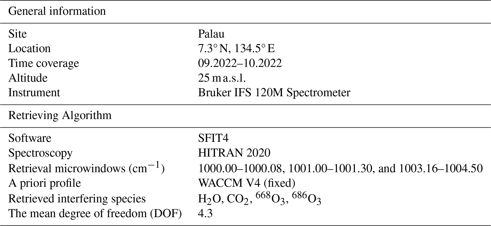
Since 2015, the Institute of Environmental Physics (IUP), University of Bremen, and Alfred-Wegener-Institut (AWI), Potsdam, have conducted atmospheric observations at the Palau Atmospheric Observatory (PAO) in Koror, Palau (7.3° N, 134.5° E) (Müller et al., 2024a). PAO is located on the Palau Community College (PCC) campus. The O₃ concentration was measured by solar absorption Fourier Transform infrared (FTIR) spectrometry in September and October 2022. The information of the FTIR measurement are given in Table 1. FTIR measurements have been performed in one of the PAO scientific containers using a Bruker IFS 120M spectrometer equipped with indium antimonide (InSb) since 2018. This allows to record spectra from 1900 up to 6000 cm⁻¹. In August 2022, Mercury Cadmium Telluride (MCT) was installed to cover the spectral region between 700–3000 cm⁻¹. The lower wavenumber region allows for the study of concentration profiles with higher precision, which is especially important for ozone.

Table 1 Information of FTIR ozone measurement in Palau.

The FTIR spectra are recorded at a high spectral resolution up to 0.005 cm⁻¹ by pointing the solar tracker at the sun during cloud-free weather conditions. The weather conditions can be actively monitored by the sky camera mounted above the window of the laboratory container to minimize the influence of clouds on solar absorption FTIR. We performed measurements throughout the day to record the spectrum from sunrise to sunset. The number of FTIR measurements contributing to each hourly bin ranges from 10 to 55, with the highest sampling between 11:00 and 14:00 LT. Each hourly bin includes measurements from multiple independent days (typically 3–10 d h⁻¹, see Appendix A). The spectra collected after 17:00 LT were excluded from our analysis due to shading from a tree adjacent to the laboratory container. The measurements during the campaign period were grouped by hour and averaged to evaluate the diurnal cycle of O₃. Therefore, we successfully obtained the ozone daytime diurnal cycle from 07:00 to 16:00 LT.

The retrieval of trace gas concentrations from solar absorption FTIR spectra was performed using SFIT-4 (Spectra Least Squares Fitting) software. Spectral line parameters were taken from the high-resolution transmission molecular absorption database version 2020 (HITRAN2020) (Gordon et al., 2022). A priori profiles were kept constant for the campaign and were from the Whole Atmosphere Community Climate Model (WACCM V4). O₃ was retrieved in three microwindows: 1000.00–1000.08, 1001.00–1001.30, and 1003.16–1004.50 cm⁻¹ with a simultaneous fit of H₂O and other interfering species (Table. 1), retrieval strategy is consistent with the the Network for the Detection of Atmospheric Composition Change (NDACC) framwork (Vigouroux et al., 2015).

To quantify tropospheric ozone, we use the part of the retrieval corresponding to the tropospheric degree of freedom (DOF≈1), whose associated partial column averaging kernel (PC AVK) spans the vertical range from the surface to 10.2 km (see Fig. 1a, red curve). The vertical range we use in this study represents the low troposphere in the tropical region. This layer is used to calculate the tropospheric dry-air partial column–averaged mole fractions of ozone, $X_{{\mathrm{O}}_{\mathrm{3}},p}$. The tropospheric $X_{{\mathrm{O}}_{\mathrm{3}},p}$ is calculated as:

$$\begin{array}{}\text{(1)}& {\displaystyle }{\displaystyle }{X}_{{\mathrm{O}}_{\mathrm{3}},p}={\displaystyle \frac{{\text{PC}}_{{\mathrm{O}}_{\mathrm{3}},p}}{{\text{PC}}_{\text{dry}}^{\text{air},p}}}={\displaystyle \frac{{\text{PC}}_{{\mathrm{O}}_{\mathrm{3}},p}}{{\text{PC}}_{\text{wet}}^{\text{air},p}-{\text{PC}}_{{\mathrm{H}}_{\mathrm{2}}\mathrm{O},p}}},\end{array}$$

where ${\text{PC}}_{{\mathrm{O}}_{\mathrm{3}},p}$, ${\text{PC}}_{\text{wet}}^{\text{air},p}$, and ${\text{PC}}_{{\mathrm{H}}_{\mathrm{2}}\mathrm{O},p}$ are the partial columns (in molecules cm⁻²) of ozone, wet air, and water vapor, respectively, over the vertical range p=0.2–10.2 km. $X_{{\mathrm{O}}_{\mathrm{3}},p}$ represents the dry-air partial column-averaged mole fraction of ozone, which is equivalent to a column-weighted mean mixing ratio (ppb) calculated by dividing the ozone partial column by that of the dry air. This approach is adopted to facilitate direct comparison with ozonesonde profiles and model outputs. For simplicity, $X_{{\mathrm{O}}_{\mathrm{3}},p}$ is hereafter referred to as the tropospheric ozone column-averaged mole fraction (TOC in ppb), over 0.2–10.2 km. Noting that its unit (ppb) distinguishes it from the total column abundance expressed in Dobson Units (DU). The altitude range is consistent with previous FTIR studies defining TOC over 0–10 km (e.g. Schneider et al., 2008; Vigouroux et al., 2008).

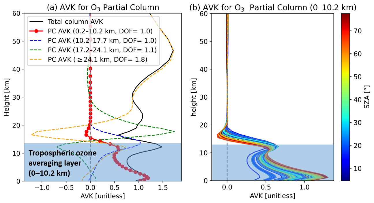
Figure 1 (a) Partial column averaging kernels (PC AVKs) of O₃ for different retrieval layers on 1 October 2022. The solid black line shows the total column AVK. Colored dashed lines indicate the PC AVKs corresponding to different degrees of freedom (DOFs): 0.2–10.2 km (DOF=1.0, red marked), 10.2–17.7 km (DOF=1.0, blue), 17.7–24.1 km (DOF=1.1, green), and ≥24.1 km (DOF=1.8, orange). Red markers highlight the PC AVK for the tropospheric ozone partial column (0.2–10.2 km), which is the focus of this study. (b) Sensitivity of the first layer PC AVK (0.2–10.2 km) during the measurement period varies with solar zenith angle (SZA). Each colored line corresponds to a retrieval at a specific SZA, with the color scale on the right.

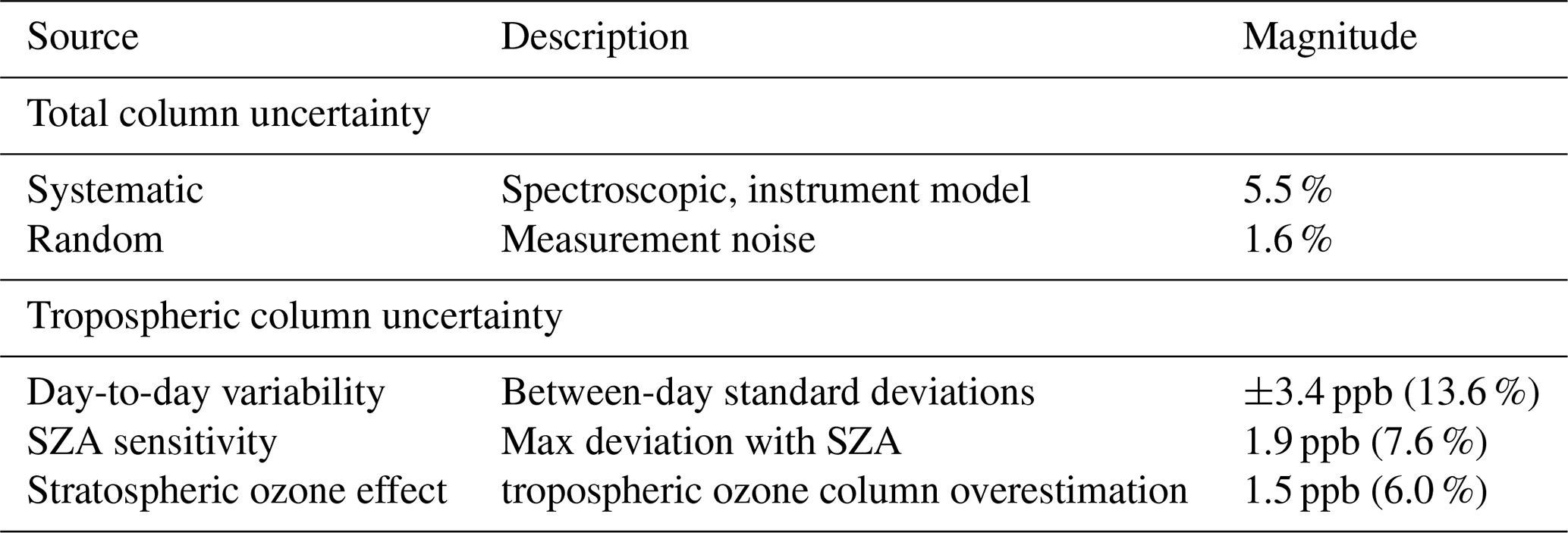
The uncertainty budget of our ozone retrievals includes different types of contributions as shown in Table 2. For the total column, systematic uncertainties from spectroscopy and instrument modeling amount to about 5.5 %, while random noise contributes 1.6 %. For the tropospheric column, the estimated uncertainties are of a different nature and therefore not directly additive. Day-to-day variability (±3.4 ppb) reflects the representativeness of the retrievals.

Table 2 Summary of ozone column uncertainties, including total column relative errors and tropospheric partial column (0–10 km) absolute uncertainties.

When interpreting the diurnal pattern from FTIR-derived TOC, two aspects require consideration. First, the FTIR-derived TOC is the integration over 0.2–10.2 km, and this inevitably dampens near-surface variability, assuming there is little variability of ozone in the free troposphere over Palau in a pristine oceanic region, like the TWP. This compromises the representation of boundary-layer changes in the integrated TOC. Second, besides this vertical smoothing, other sources of uncertainty also affect the retrieved TOC, such as solar zenith angle (SZA) dependence and residual stratospheric influence.

As shown in Fig. 1a, the PC AVK of the first layer is highly sensitive within the 0.2–10.2 km range, indicating high information content. This supports using the part of the retrieval corresponding to the tropospheric degree of freedom (DOF≈1) to represent the TOC. Moreover, the PC AVK is the highest below 2 km (PC AVK ≈1.0), and decreases with altitude (Fig. 1a, red line). This indicates that TOC mainly reflects near-surface information. The same feature was observed for all PC AVK during the measurement period (Fig. 1b). The maximum sensitivity always lies near the surface, where most of the diurnal variation occurs. From previous aircraft observations, no discernible diurnal ozone variations were found above 750 hPa (Petetin et al., 2016). Thus, consistent with the PC AVK, the FTIR-derived tropospheric ozone column primarily captures near-surface ozone variability, although vertical integration over the column reduces the apparent diurnal amplitude. We estimate that the TOC retains only about 40 % of the near-surface variability (see Appendix B3).

From FTIR-derived TOC to interpret the diurnal cycle, the SZA dependency of the measurements should also be considered. As shown in Fig. 1b, the sensitivity of the FTIR measurements varies with SZA. We estimate the resulting SZA-induced uncertainty of a maximum deviation of 1.9 ppb (7.6 %), see details of the quantifying method in Appendix B1. To validate the FTIR TOC diurnal cycle, we further compare the retrievals with model simulations and ozonesonde observations.

However, the PC AVK does not drop sharply above 10.2 km but gradually decays, reaching near-zero only around 20 km (Fig. 1). This indicates residual sensitivity above the defined TOC layer, which can lead to vertical smoothing–induced leakage of stratospheric ozone to the TOC. Given that ozone mixing ratios increase with altitude from the upper troposphere, this leakage results in an overestimation bias of approximately 1.5 ppb (6.0 %) in the retrieved TOC, see Appendix B2. Together, these values characterize the expected range and type of uncertainty, but they do not compromise the detection of the observed diurnal pattern.

2.2 GEOS-Chem Model Simulations

O₃ concentrations were simulated using the global 3-D chemical transport model GEOS-Chem (version 13.4.0, classic, The International GEOS-Chem User Community, 2022; Bey et al., 2001), with the full-chemistry module. The model was driven by meteorological fields from the Modern-Era Retrospective Analysis for Research and Applications, Version 2 (MERRA-2), provided by the NASA Global Modeling and Assimilation Office (GMAO).

Emissions were handled using the Harmonized Emissions Component (HEMCO; Keller et al., 2014; Lin et al., 2021). Lightning NO_x (LNO_x) emissions were taken from the GEOS-Chem standard configuration (HEMCO Lightning NOx v2014-07), based on cloud-top height parameterizations and described in the official GEOS-Chem HEMCO archive.

Moreover, we conducted two sensitivity simulations, one LNO_x emission is turning off and one LNO_x is doubling, to show lightning effect on ozone formation and atmospheric oxidation. Simulations cover the period 2020–2022, using a horizontal resolution of 2°×2.5°, 72 vertical levels from the surface to 10 hPa, with time steps of 10 min for transport and 20 min for chemistry. Model output was archived hourly.

2.3 Intercomparison

O₃ concentrations from FTIR measurements, ozonesonde profiles, and model simulations are compared in this study to evaluate the consistency between observations and model outputs. To ensure a fair comparison, we use model results from the full chemistry simulation and account for the vertical sensitivity of the FTIR retrievals by applying the retrieval AVK.

The retrieval sensitivity is described by the AVK matrix A and the a priori profile x_a, both of which affect how true atmospheric profiles are represented in the FTIR product (Palm et al., 2005; Rodgers, 2000). To make the model or ozonesonde profiles x_m comparable with the FTIR retrievals, they are first smoothed using the following equation:

$$\begin{array}{}\text{(2)}& {\displaystyle }{\displaystyle }{\mathit{x}}_{\mathrm{s}}={\mathit{x}}_{\mathrm{a}}+\mathbf{A}({\mathit{x}}_{\mathrm{m}}-{\mathit{x}}_{\mathrm{a}}),\end{array}$$

where x_s denotes the smoothed profile that incorporates the FTIR sensitivity characteristics. To ensure consistency in the application of the AVK, all model and ozonesonde profiles were interpolated to the vertical grid of the FTIR retrieval. This step is essential, as the AVK matrix A is defined on the FTIR retrieval levels, and applying it directly to profiles on different vertical coordinates would lead to incorrect smoothing. Linear interpolation was used in pressure space, as it preserves the structure of atmospheric layers and is commonly applied in intercomparison studies e.g. Ridder et al. (2012); Schneider et al. (2008).

After smoothing, the dry-air partial column-averaged mole fraction of ozone, $X_{{\mathrm{O}}_{\mathrm{3}},p}$, is computed for both the FTIR retrievals and the model or ozonesonde profiles as mentioned in Sect.2.1 Eq. (1). The partial column is defined from the surface up to 10.2 km, corresponding to the first layer of the FTIR retrieval product, as described in Sect. 2.1. This consistent vertical integration ensures that differences reflect physical and chemical discrepancies rather than vertical resolution mismatches.

2.4 Trajectory simulation

To investigate the large-scale transport influencing ozone variability over Palau, we performed air-parcel trajectory analyses using the Hybrid Single-Particle Lagrangian Integrated Trajectory (HYSPLIT) model developed by NOAA's Air Resources Laboratory (Stein et al., 2015). The calculations were driven by meteorological fields from the Global Data Assimilation System (GDAS; Kanamitsu, 1989), which provides global coverage at 1°×1° horizontal resolution and 3-hourly temporal frequency. GDAS data are widely used in regional and long-range transport studies.

Backward trajectories were initialized at the location of the Palau Atmospheric Observatory for three starting altitudes: the surface, 5, and 10 km. These levels represent conditions within the marine boundary layer, the lower free troposphere, and the upper portion of the FTIR retrieval range, respectively. Each trajectory was traced 10 d backward in time to identify the dominant pathways and potential source regions influencing the observed ozone during the FTIR campaign.

The resulting trajectory ensemble provides a dynamical context for interpreting the tropospheric ozone signal by indicating whether the sampled air masses originated from remote oceanic regions, convective outflow, or areas with continental influence. While GDAS does not fully resolve small-scale boundary-layer mixing, it reliably captures the larger-scale circulation patterns that dominate transport in the TWP, making it suitable for assessing the origin and history of air masses arriving at Palau.

2.5 Data

2.5.1 Ozonesonde Observations

To support and evaluate the FTIR ozone retrievals, we use in situ vertical ozone profiles from ozonesonde launches at the PAO. Routine ozonesonde observations at this site have been conducted since 2016, as part of a long-term monitoring effort to characterize tropospheric composition and transport in the TWP (Müller et al., 2024a). These observations provide high-vertical-resolution measurements of ozone, pressure, temperature, and relative humidity from the surface to the lower stratosphere.

During our FTIR measurement period (in September and October 2022), three ozonesonde launches can be matched with the measurement time of FTIR within the same day. We identified the FTIR measurements closest in time to each launch and used these matched pairs in comparison. To ensure consistency with the FTIR retrieval characteristics, when we make intercomparison between the TOC from FTIR and ozonesonde measurements, the ozonesonde profiles were smoothed using the FTIR AVK following the Eq. (2) as previously described in Sect. 2.3. For quantitative comparison, we calculated the dry-air partial column ozone from the surface to 10.2 km for each smoothed sonde profile, using the dry-air number density derived from pressure and temperature. This provides column amounts in molecules cm⁻², consistent with the integration range and units used in the FTIR analysis. This allowed a direct assessment of the agreement between FTIR retrievals and in situ measurements in the troposphere under matched temporal and vertical sampling conditions.

In addition to the matched-pair intercomparison with AVK-smoothed sonde profiles, we also examined whether the FTIR captures a consistent diurnal pattern by including all ozonesonde launches from September to October during 2020–2022. In total, 12 sondes were launched on 12 different days during this period. They were released at varying times of day, providing a general overview of diurnal variability during these months. However, no launches were performed in the morning due to operational constraints. As a result, ozonesonde observations do not cover the morning period, which is instead captured by the FTIR measurements.

Because the number of matched pairs is limited, no AVK smoothing was applied in this analysis. However, a key challenge arises from the different measurement characteristics: FTIR retrievals are influenced by the AVK and have different sensitivity across the retrieval layer, whereas ozonesondes provide in situ profiles with uniform sensitivity. To enable a qualitative comparison of diurnal variability, we therefore focused on relative rather than absolute values. Specifically, we calculated the normalized anomaly of each dataset as

$$\begin{array}{}\text{(3)}& {\displaystyle }{\displaystyle }{x}^{\prime }={\displaystyle \frac{x-\overline{x}}{\overline{x}}}\end{array}$$

where x represents the hourly measurements from FTIR retrievals or ozonesonde, and $\overline{x}$ is the mean over the altitude of the respective dataset. This normalization x^′ is used to estimate the relative deviation from the mean value of each measurement. It removes the offset in absolute magnitude between the two instruments and highlights their relative deviations from the mean, allowing a comparison of the diurnal pattern of ozone.

2.5.2 Ozone precursor

The tropospheric ozone column from satellite is from the Ozone Monitoring Instrument/Microwave Limb Sounder (OMI/MLS) product (Ziemke et al., 2006). The OMI/MLS product is the residual of the OMI total ozone column and the MLS stratospheric ozone column, available from October 2004–December 2024 in monthly means as gridded (1°×1°). The tropospheric NO₂ column was from the Quality Assurance for Essential Climate Variables (QA4ECV) project version 1.1 level 3 (L3) product from OMI (2004–2017), from GOME-2(A) (2007–2016), from SCIAMACHY (2002–2012), in monthly means as 0.125°×0.125° gridded (Boersma et al., 2017a, b, c, 2018). The tropospheric formaldehyde (HCHO) column was also from the QA4ECV project version 1.0 Level 3 (L3) product based on OMI measurements available between October 2004 and December 2020, monthly means as 0.05°×0.05° gridded available (Lin et al., 2021; De Smedt et al., 2018). The total column of CO was derived from the IASI satellite, also from the QA4ECV project. We use the level 3 (L3) products, it is available from 2007 to present, with monthly means 1°×1° gridded available (LATMOS, 2013).

2.5.3 Cloud effective radius

We used daily gridded cloud effective radius data from the MODIS/Aqua Level-3 product (CLDPROP_D3_MODIS_Aqua; Platnick et al., 2019), which provides globally gridded cloud optical and cloud-top properties retrieved using a unified algorithm applicable to both MODIS and VIIRS sensors, ensuring continuity across instruments. The analysis focused on the cloud effective radius at a spatial resolution of 1°×1° for the months of September and October 2022. The MODIS CLDPROP Level-3 dataset has been extensively validated and widely used to investigate large-scale cloud microphysical properties, aerosol–cloud interactions, and climate-related variability (e.g. King et al., 2013; Platnick et al., 2021).

2.5.4 Lightning

Lightning data are from the ground-based World Wide Lightning Location Network (WWLLN), providing a regional view of lightning activity during the Palau campaign period. The data were obtained from the publicly available WWLLN climatology archive (e.g. Virts et al., 2013; Kaplan and Lau, 2021, 2022), which provides globally gridded lightning stroke densities based on very low frequency (VLF) detections from a network of ground-based stations. Only strokes detected by at least five stations are retained to ensure high location accuracy (e.g. Hutchins et al., 2012; Navarro et al., 2024), and the overall performance of WWLLN has been evaluated against satellite-based observations, demonstrating reliable detection efficiency and spatial accuracy (e.g. Rudlosky and Shea, 2013). This monthly gridded product has been widely used to study large-scale lightning patterns (e.g. Amador and Arce-Fernández, 2022).

3 Results

3.1 Tropospheric Ozone Measurement by FTIR and Comparison with Ozonesondes

We present tropospheric ozone observations over Palau using FTIR spectroscopy. Figure 2 shows the time series of daily mean TOC derived from FTIR measurements, compared with GEOS-Chem model simulations and ozonesonde observations. The FTIR observations reveal very low tropospheric ozone levels, with an overall daily mean of 24 ppb. GEOS-Chem simulations, smoothed with the same AVK, yield a mean of 22.85 ppb over the campaign period. The ozonesonde-based TOC shows good agreement with the FTIR measurements, further validating the reliability of the retrievals. As shown in Fig. 2b, the differences between the model and FTIR observations generally vary within ±5 ppb, indicating that the model captures the day-to-day variability reasonably well. Overall, the model underestimates the absolute concentrations.

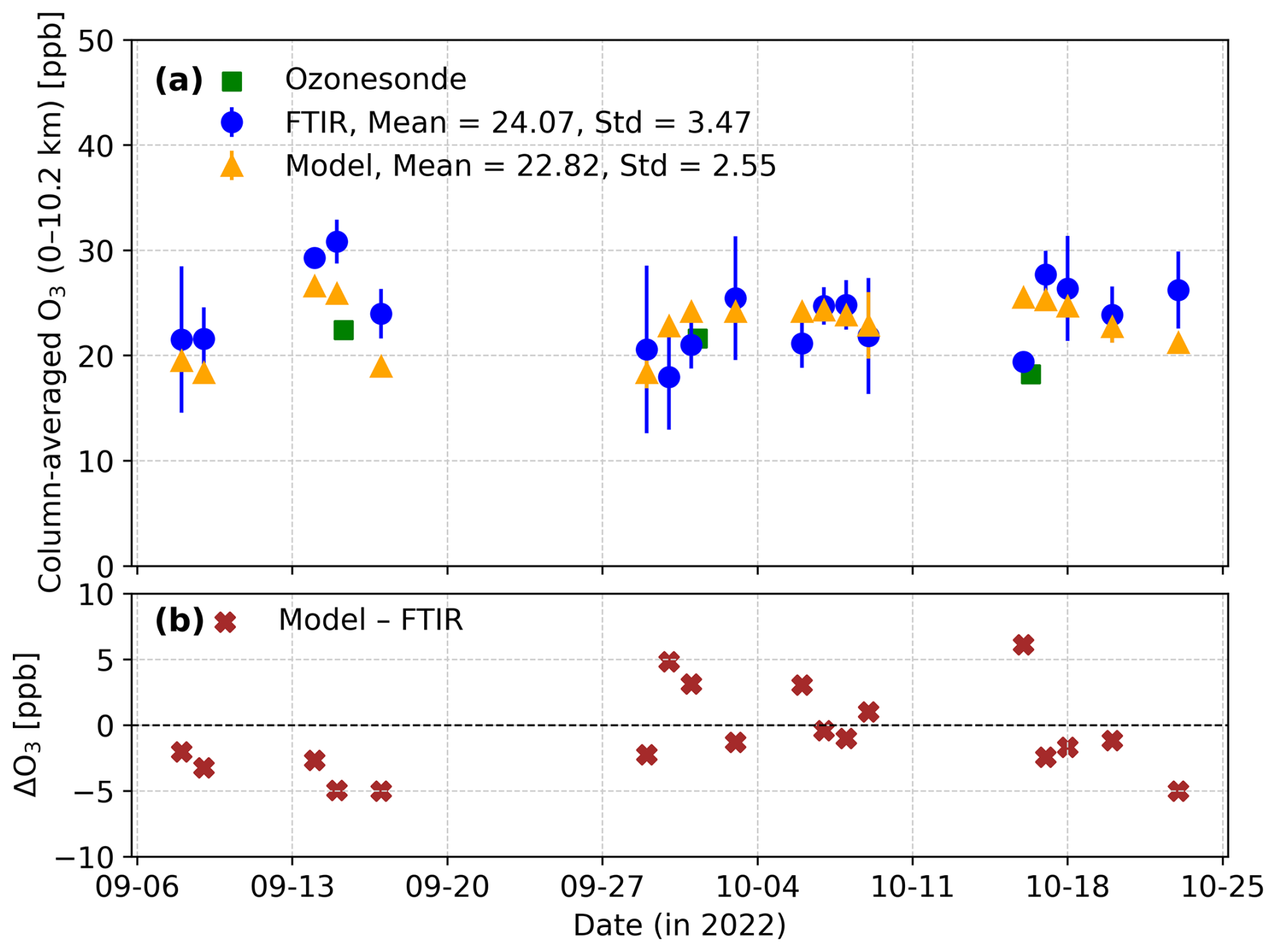
Figure 2 (a) Time series of tropospheric O₃ columns (ppb) from FTIR measurements, smoothed GEOS-Chem simulations, and smoothed ozonesonde profiles. (b) Daily differences between GEOS-Chem and FTIR (model – FTIR). All values represent dry-air partial columns averaged from the surface to 10.2 km. Ozonesonde and model profiles are interpolated to the FTIR grid and smoothed with the FTIR AVK before integrating 0–10.2 km to TOC.

Building upon the time series analysis presented above, we next focus on the daytime diurnal variability of tropospheric ozone derived from the high-temporal-resolution FTIR observations. Because of the continuous solar absorption measurements throughout the day, the FTIR provides hourly retrievals between 07:00 and 16:00 LT. These retrievals can be used to derive the diurnal pattern of the O₃ measurements, as described in Sect. 2.1. Figure 3 summarizes the diurnal behaviour: panel a shows the FTIR-derived tropospheric ozone column (TOC) together with GEOS-Chem simulations, while panel b presents normalized ozonesonde ozone profiles at different hours for evaluating the FTIR-derived diurnal pattern.

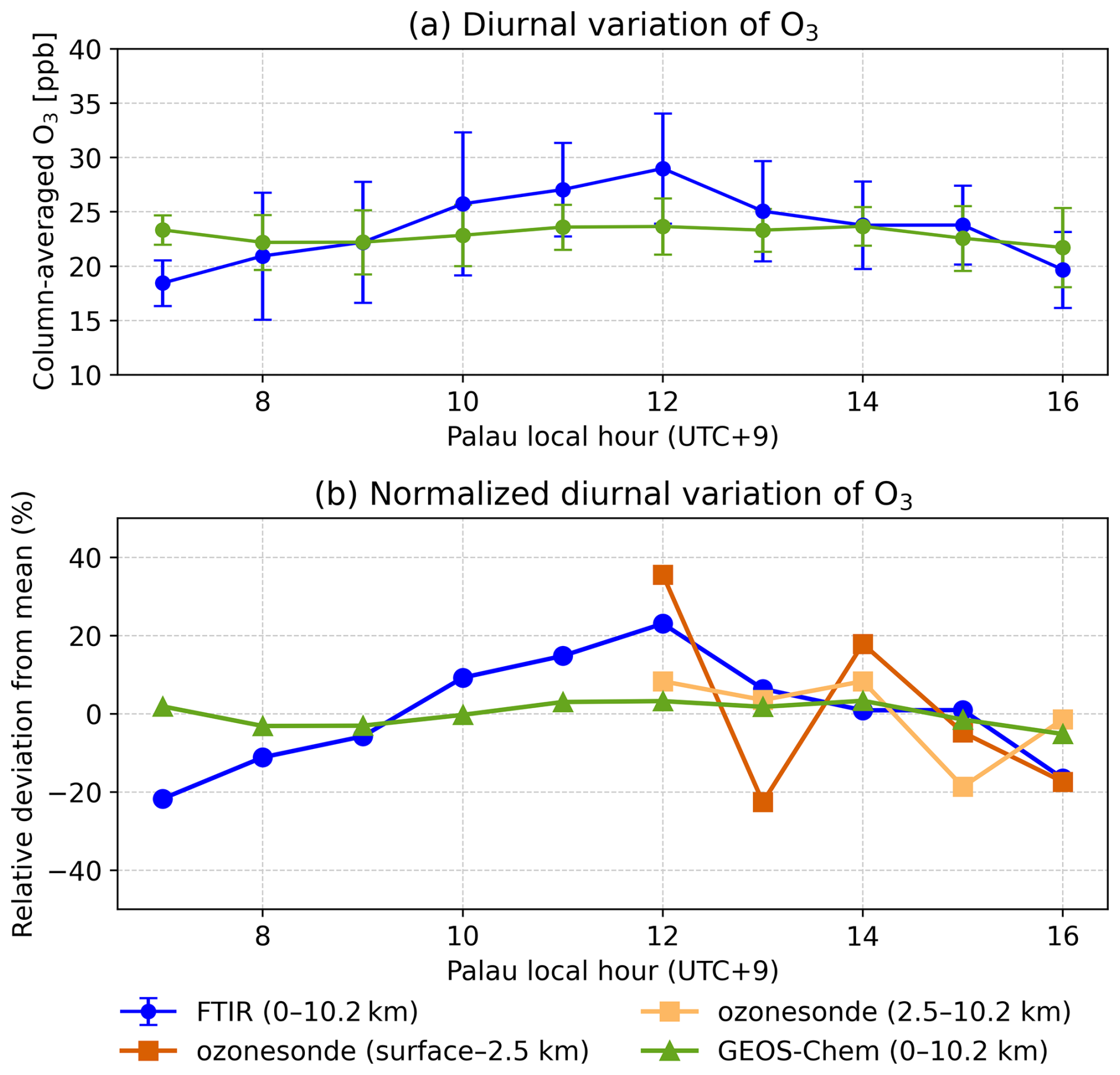
Figure 3 (a) Diurnal variation of tropospheric column of O₃ (TOC) from FTIR measurement and GEOS-Chem (smoothed with AVKs). Error bars denote ±1σ variability within each hourly bin. (b) Normalized diurnal variation of O₃ from FTIR TOC, GEOS-Chem, and ozonesonde volume mixing ratios from surface–2.5 and 2.5–10.2 km. Normalized values are calculated relative to the mean of each dataset (see Sect 2.5.1). Absolute values of ozonesonde hourly mean are shown in Appendix C.

Figure 3a shows the daytime diurnal cycle of tropospheric ozone from FTIR measurements compared with GEOS-Chem simulations. FTIR data show an increase in ozone in the early morning, peaking around noon, followed by a decline in the afternoon. Figure 3 also compares the FTIR diurnal cycle with the GEOS-Chem simulation, time matched to FTIR measurements and smoothed. Compared with observational data, the model shows a much flatter pattern. Simulations without applying AVK smoothing display an even flatter diurnal variation with ozone concentrations remaining nearly constant throughout the day (see Appendix B1). Note that Fig. 3a shows TOC derived from model profiles after AVK smoothing. The weak midday enhancement of about 2 ppb mainly results from the AVK smoothing effect associated with changes in solar zenith angle during the day. This indicates that the model fails to capture both the midday peak and the amplitude of the observed variations simultaneously. It also overestimates ozone in the early morning and late afternoon. Consequently, the simulated ozone diurnal cycle appears muted compared to observations. While the model captures the characteristic diurnal variability of photochemical radicals, the resulting net ozone change is insufficient to drive a discernible amplitude in the column (see Appendix B1 and Fig. B1 for details on radical concentrations). This discrepancy likely arises from the coarse horizontal resolution and parameterized boundary-layer dynamics, which cannot catch the localized mixing or production mechanisms in the TWP. In addition, simplified representations of diurnal emissions and photolysis may further damp small-scale variability, as suggested by the FTIR and ozonesonde diurnal pattern in Fig. 3b.

Figure 3b compares normalized ozone variations from FTIR and ozonesonde measurements (see Sect. 2.5.1). Because the FTIR retrievals have different sensitivity across altitude, the AVK must be considered when making such comparisons (Schneider et al., 2008; Rodgers and Connor, 2003). Given the limited number of time-matched observations, we used normalized hourly averages to remove absolute differences between datasets, see Sect. 2.5.1. This approach enables a qualitative comparison of diurnal variability based on relative changes without applying smoothing to the ozone sounding profiles. Relative deviations from the mean were calculated for each dataset (Eq. 3), and the resulting normalized diurnal variation is shown in Fig. 3b. The absolute hourly mean plot of ozonesonde is shown in Appendix A. The ozonesonde data also exhibit a midday enhancement, though less pronounced than in the FTIR measurements, followed by a discernible afternoon decline and a more dispersed distribution in both the near-surface layer (below 2.5 km) and the free troposphere (2.5–10 km). These results highlight the inherent challenges in comparing FTIR and ozonesonde observations due to their different vertical sensitivities. Even without sufficient morning ozonesonde launches and without AVK smoothing of profiles, the normalized O₃ from different datasets still provides indirect evidence for the pattern of midday peak and the afternoon decline. The error bars in Fig. 3a indicate an hourly variability of approximately 2–6 ppb (±1σ). The daytime diurnal variation of tropospheric ozone measured by FTIR is on the order of 6–8 ppb, but this magnitude should be interpreted as a lower limit of near-surface ozone variability, as the FTIR retrieval represents a vertically integrated tropospheric column (0–10 km) with a reduced peak-to-peak amplitude.

This interpretation is supported by the ozonesonde observations in Fig. 3b, which show larger ozone variability near the surface than in the free troposphere, where photochemical production and dry deposition are weaker above approximately 750 hPa (about 2.5 km) (Petetin et al., 2016). Accounting for the solar zenith angle (SZA) effect, which leads to an overestimation of the apparent diurnal amplitude by about 1.9 ppb (Appendix B1), the FTIR-derived peak-to-peak variation is approximately 4–6 ppb. Considering the ∼40 % damping of near-surface variability in the vertically integrated tropospheric ozone column (Appendix B3), this implies a near-surface diurnal ozone amplitude on the order of ∼15 ppb.

3.2 Low ozone and precursors in Palau

Palau is located in the TWP, a region characterized by persistently low tropospheric ozone concentrations (Rex et al., 2014; Ridder et al., 2012). Observations show that daytime ozone levels typically remain between 10–30 ppb from July until October (Müller et al., 2024b), among the lowest values globally. To examine the origin and transport pathway of air masses influencing Palau, we computed 10 d backward trajectories using the HYSPLIT model. Most trajectories remain below 10 km (Fig. 4a), indicating that transport occurs within the free troposphere. Trajectories longer than 8 d predominantly originate from the central Pacific, following easterly circulation across the Pacific, with trade winds dominating the lower troposphere and additional contributions from large-scale tropical circulation at higher altitudes (Fig. 4b). This flow pattern is typical for the September–October period, which lies in the transition between the southwest monsoon and the establishment of the northeast trade wind regime (Müller et al., 2024b; Sun et al., 2023). During this period, the TWP is mainly influenced by persistent marine inflow from the east, resulting in minimal continental influence. Ozone lifetimes are on the order of 10–20 d in the free troposphere (Prather and Zhu, 2024), but considerably shorter in the marine boundary layer and increasing with altitude. (about 5 d; Liu et al., 1983; Kley et al., 1997). Thus, these air parcels are expected to retain their low ozone concentrations upon arrival. In addition, backward trajectories show that during the 2–6 d before arrival, air masses confined mostly below 1.5 km originate in the western Pacific, reflecting additional regional marine contributions (Fig. 4a and b). Together, these results suggest that both long-range and regional transport of ozone-poor air masses contribute to the persistently low tropospheric ozone observed over Palau.

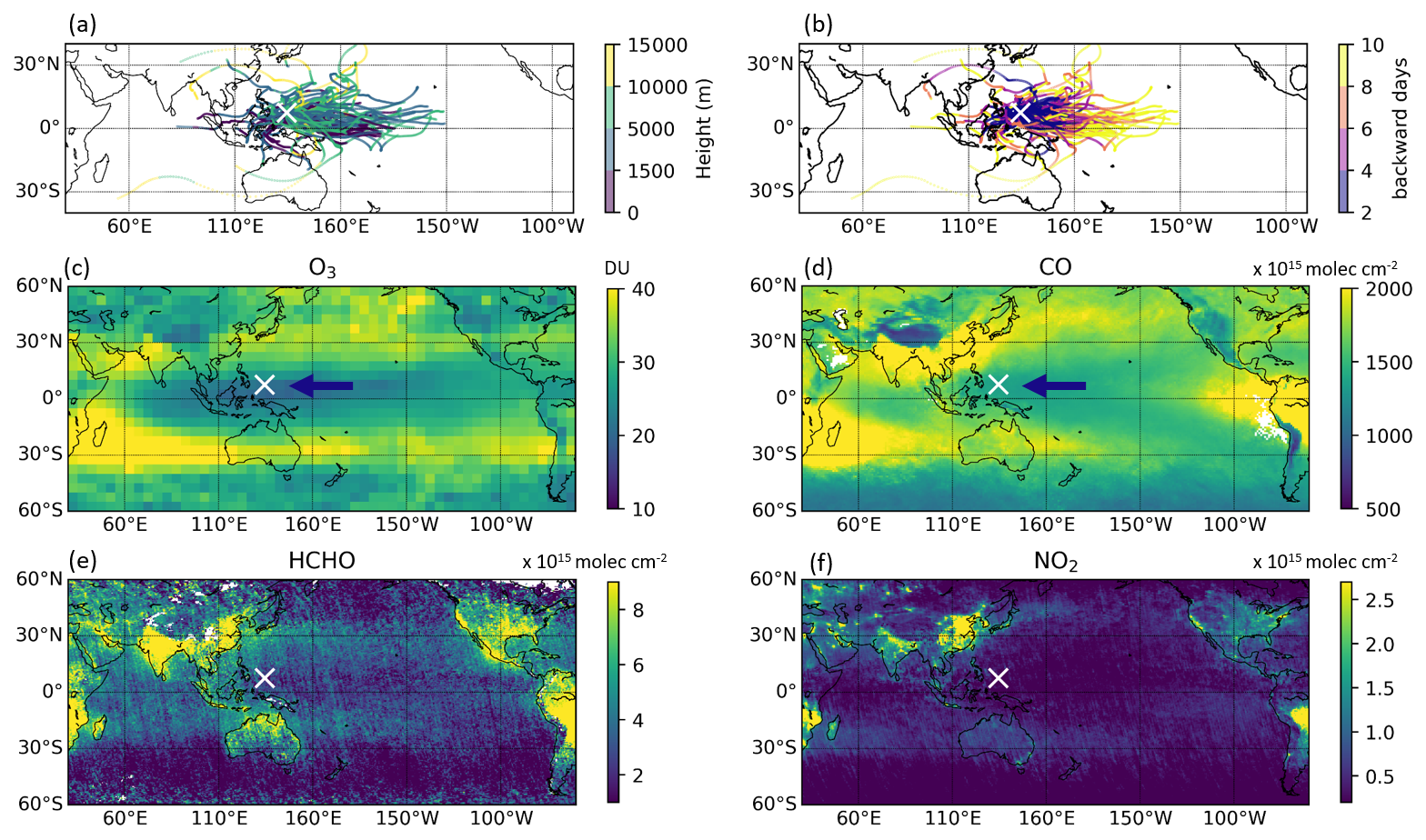
Figure 4 (a–b) Ten-day backward trajectories initiated from Palau, color-coded by (a) altitude (m) and (b) backward time (d). (c–f) Satellite-derived tropospheric column of (c) O₃, (d) CO, (e) HCHO, and (f) NO₂. The white cross marks the location of Palau. The arrow in panels (c) and (d) indicates the mean transport pathway during the study period based on trajectory simulations.

Satellite retrievals support this interpretation. A broad ozone minimum is evident over the western Pacific warm pool (Fig. 4c), coinciding with low column densities of major precursors: CO (Fig. 4d), HCHO (Fig. 4e), and NO₂ (Fig. 4f). The scarcity of these precursors in both the lower and free troposphere points to a suppressed photochemical ozone production regime. The lack of precursors arises from weak local emissions and the continuous inflow of clean marine air from the eastern Pacific. In addition, the interhemispheric convective zone (ITCZ) over the TWP during the campaign coincided with strong precipitation bands (Sun et al., 2025), which likely enhanced the washout of precursors. Enhanced humidity in the tropical troposphere promotes ozone loss via OH chemistry. At the same time, precipitation efficiently removes soluble species such as HCHO and nitrogen reservoir species produced from NO_x oxidation (e.g. HNO₃), indirectly reducing NO_x availability and suppressing ozone production. Trajectory analyses confirm that air masses reaching Palau predominantly follow oceanic pathways with minimal continental influence, as mentioned before. This is consistent with (Müller et al., 2024b), who showed similar oceanic transport patterns in the 5–10 km layer but predominant during September and October. These pathways align with regions of consistently low CO and ozone concentrations across the tropical Pacific (Fig. 4c and d). In contrast, NO₂ has a short atmospheric lifetime and is not efficiently transported over long distances, such that its low abundance near Palau reflects weak local and regional NO_x sources (Fig. 4f). HCHO, while also short-lived, is primarily produced locally through VOC oxidation, and its low abundance therefore indicates weak photochemical activity under pristine marine conditions (Fig. 4e), further limiting in situ ozone formation. The low NO₂ columns also suggest minimal contributions from lightning or other episodic NO_x sources, reinforcing the interpretation of limited photochemical ozone production.

3.3 Microphysical suppression of lightning and ozone formation

In the maritime TWP, despite low lightning frequency, lightning-generated NO_x remains an important free-tropospheric ozone source. We therefore investigate the microphysical conditions influencing lightning initiation, in addition to dynamical and chemical factors. Figure 5a shows the spatial distribution of lightning stroke density from WWLLN observations, confirming that lightning activity near Palau is lower than over the Maritime Continent or northern Australia. Although isolated lightning events do occur over the open ocean (Fig. 5a), they are sparse and less frequent, indicating that meteorological and microphysical environments in this region are inherently unfavorable for intense convective electrification. Observational evidence for marine convection without lightning has been reported in several studies, including Nussbaumer et al. (2021) over the tropical Atlantic and the PEM-West campaign (Crawford et al., 1997), which found that such convection favors the washout of NO_x derivatives.

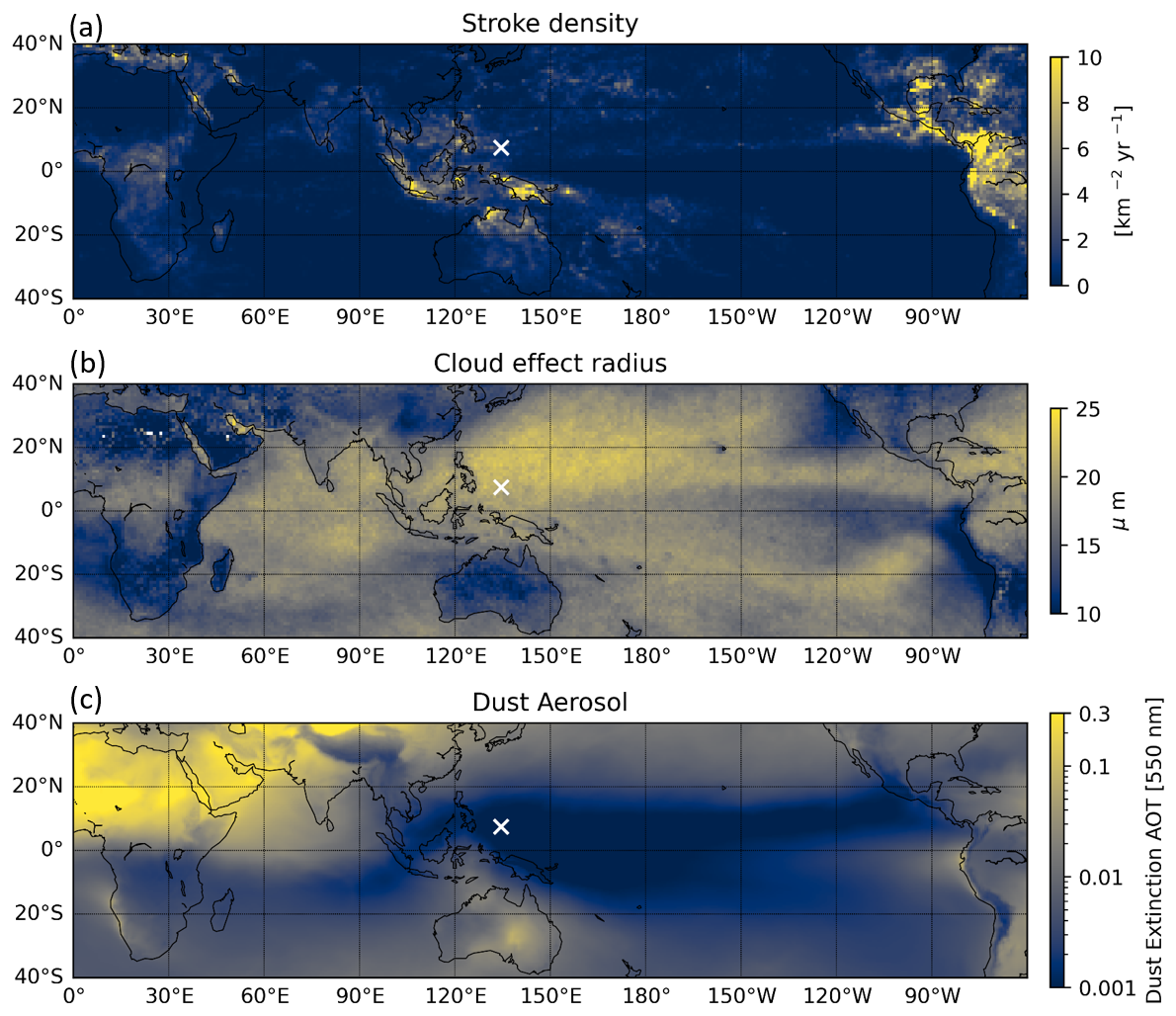
Figure 5 Spatial distribution of (a) annual mean lightning stroke density (${\mathrm{km}}^{-\mathrm{2}}{\mathrm{yr}}^{-\mathrm{1}}$) from WWLLN, (b) MODIS satellite derived cloud effective radius (µm) and (c) dust aerosol optical extinction (AOT) at 550 nm from MERRA-2 reanalysis. The white cross marks the location of Palau.

The MODIS-derived cloud effective radius is shown in Fig. 5b. Over the warm pool region, cloud droplets are generally larger, which is typically associated with enhanced precipitation water content and reduced ice water content (Braga et al., 2021). These conditions promote warm-rain processes and inhibit the development of ice particles, thereby weakening charge separation and suppressing lightning activity (Huang et al., 2025). Figure 5c displays the dust aerosol optical thickness over the TWP, showing low dust loadings above Palau. In contrast to continental outflow regions, the central Pacific air column is nearly devoid of aerosol particles capable of serving as ice nuclei. This lack of ice nuclei suppresses the formation of ice-dominant or mixed-phase clouds (Chen et al., 2024a), reducing the likelihood of charge separation and lightning initiation (Han et al., 2021). Low aerosol concentrations favor the formation of larger cloud droplets, which reduces lightning activity and lowers NO_x production. This, in turn, diminishes ozone levels in the upper free troposphere and illustrates the tight coupling between aerosol microphysics, cloud dynamics, and atmospheric chemistry. It provides an additional causal chain rooted in microphysical processes, through which precursor scarcity is further reinforced, complementing the direct explanations of weak anthropogenic influence and efficient washout (Sect. 3.2). In this view, the low precursor abundances over Palau arise not only from a dynamically clean marine environment but also from suppressed lightning NOx production linked to the paucity of ice nuclei and mixed-phase clouds.

While this interpretation is supported by the observed patterns, the spatial differences (Fig. 5) between dust aerosol, cloud effective radius, and lightning activity suggest that more complex microphysical processes may also be at play. This points to the possibility of additional factors influencing lightning production in marine convective systems, such as variations in updraft strength, cloud ice content, freezing level height, or the availability of giant cloud condensation nuclei for mixed-phase cloud (Ji et al., 2025). Importantly, the overall meteorological linkage supports the view that photochemical background conditions in tropical marine regions are not only chemically pristine but also dynamically regulated by aerosol–cloud interactions.

3.4 Influence of Lightning NO_x on Regional Ozone

To quantify the role of lightning-produced nitrogen oxides (LNO_x) in modulating tropospheric ozone over Palau, we performed two sensitivity simulations using the GEOS-Chem model by turning off and doubling LNO_x emissions (Fig. 6). As shown in Sect. 3.3, lightning activity is negligible in the TWP region. Therefore, substantial perturbations to LNO_x emissions, near-surface and free-tropospheric NO mixing ratios over the TWP exhibit little response (Fig. C1c–i). In contrast, pronounced responses to LNO_x perturbations are evident over lightning-active regions such as northern Australia and the Maritime Continent.

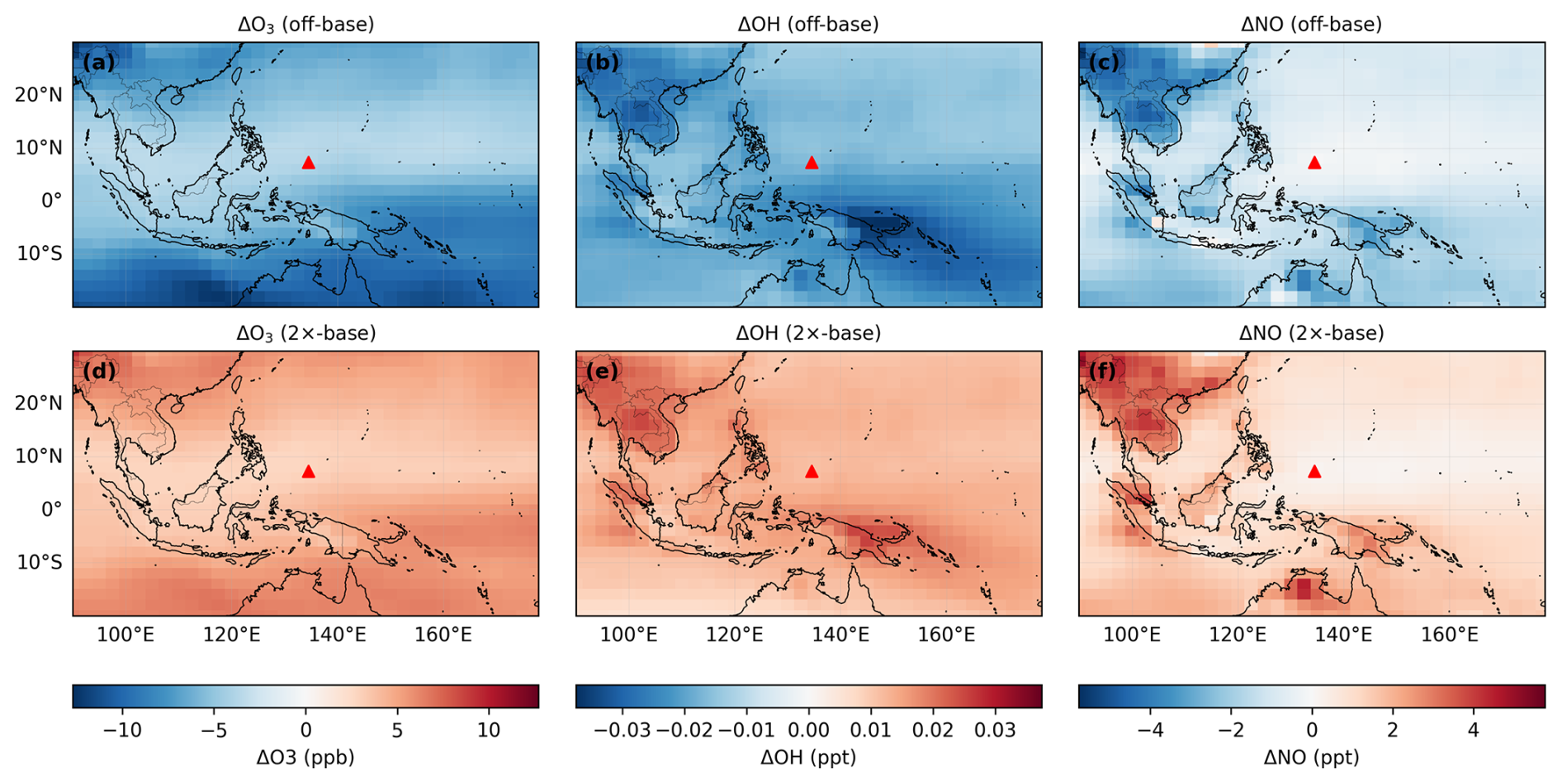
Figure 6 Differences in tropospheric column–averaged mole fractions of O₃, OH, and NO dry-air between LNO_x sensitivity simulations and the base simulation. (a–c) the differences between the no-NO_x simulation and the base simulation (no NO_x minus base), and (d–f) the differences between the 2×NO_x simulation and the base simulation (2×NO_x minus base). Columns correspond to O₃, OH, and NO from left to right. The red triangle marks the location of the Palau FTIR measurement site. The absolute value of the simulation results are shown in Appendix C, Fig. C1.

The resulting ozone anomalies extend eastward into the TWP, indicating that the ozone response over Palau primarily reflects transport from nearby regions, such as northern Australia and the Maritime Continent rather than local photochemical production. As a result, removing or doubling LNO_x emissions (Fig. C1b and c) leads to modest ozone changes over the TWP, with regional differences of approximately ±5 ppb (Fig. 6a and d).

Moreover, LNO_x emissions moderately enhance regional hydroxyl radical (OH) concentrations (Fig. 6b and e), reflecting their contribution to atmospheric oxidative capacity. In the absence of LNO_x, OH levels decrease by approximately 0.02 ppt. Under clean air conditions such as the TWP, OH is mainly produced by ozone photolysis followed by the reaction of excited atomic oxygen with water vapor (Schumann and Huntrieser, 2007). Specifically, the dominant pathway is ${\mathrm{O}}_{\mathrm{3}}+h\mathit{\nu }\to \mathrm{O}{(}^{\mathrm{1}}\mathrm{D})+{\mathrm{O}}_{\mathrm{2}}$, followed by $\mathrm{O}{(}^{\mathrm{1}}\mathrm{D})+{\mathrm{H}}_{\mathrm{2}}\mathrm{O}\to \mathrm{2}\mathrm{OH}$ (Levy, 1971). While this pathway governs the primary production of OH, its regeneration depends strongly on the availability of NO through the reaction ${\mathrm{HO}}_{\mathrm{2}}+\mathrm{NO}\to \mathrm{OH}+{\mathrm{NO}}_{\mathrm{2}}$. In the absence of NO, the lifetime of HO₂ increases, yet OH recycling becomes inefficient (Gao et al., 2014), leading to a less oxidizing atmosphere and reduced photochemical ozone production efficiency.

In remote tropical regions like Palau, where anthropogenic NO_x emissions are minimal and lightning activity is strongly suppressed, lightning represents one of the few potential sources of NO_x. Our sensitivity simulations indicate that, under such conditions, the impact of LNO_x on local ozone is indirect and transport-driven rather than in situ. Although the overall influence on ozone is modest, LNO_x plays a systematic role in regulating the regional oxidative capacity, consistent with previous assessments identifying lightning as a key natural NO_x source in remote tropical atmospheres (Nussbaumer et al., 2024, 2025).

4 Discussions

Previous studies have demonstrated characteristic diurnal surface ozone cycles in both urban and remote mid-latitude regions, driven predominantly by photochemical processes. For instance, Strode et al. (2019), Bernier et al. (2019), and (Xia et al., 2021) reported daytime increases in surface ozone over the US and China, highlighting the role of local photochemistry under sufficient solar radiation and precursor availability. Similarly, observations from a remote high-altitude site in the Tibetan Plateau revealed a midday ozone maximum, further supporting the dominance of daytime photochemical production even in pristine environments (Yin et al., 2017). Our measurements in TWP exhibit a comparable diurnal pattern in the tropospheric column, with ozone peaking around noon. Comparison with near-surface ozonesonde profiles further supports the presence of a midday enhancement. It should be emphasized, however, that the FTIR retrieval provides an integrated column signal (0–10.2 km), rather than a direct measurement of the surface. If the free troposphere exhibits little or no diurnal variability, then the signal detected in the integrated column likely reflects a surface-driven cycle that appears in muted form when averaged over the full tropospheric depth. Still, the FTIR TOC measurements in Palau capture the diurnal pattern, although the peak-to-peak amplitude is underestimated. The higher AVK sensitivity in the lower troposphere (Fig. 1) ensures that surface-driven variability is retained in the column retrieval rather than being fully smoothed out. This highlights that similar analyses at other FTIR sites must carefully consider the altitude-dependent sensitivity of the retrieval (AVK), as it determines how surface-driven diurnal variability is sufficiently reflected in the integrated column.

The comparison between the GEOS-Chem model simulation and the observations in Palau shows an overall agreement in day-to-day variation, suggesting that the tropical region is reasonably well represented, consistent with findings from previous studies (Christiansen et al., 2022; Hu et al., 2017). However, it does not well capture the ozone diurnal cycle and is biased lower than the observations. This underestimation is consistent with previous evaluations of GEOS-Chem, which have also reported a low bias relative to the observations. This underestimation aligns with prior evaluations of GEOS-Chem, which have similarly reported a low bias in tropospheric ozone in both the mid-latitudes – often linked to limitations in simulating stratosphere – troposphere exchange – and in tropical regions due to active convection (Hu et al., 2017). These results highlight the need for further improvements in the model performance over the remote western Pacific, where observational constraints remain limited.

The tropospheric ozone levels in Palau are the lowest, with a mean value of 24 ppb, which is consistent with findings from previous studies. Newton et al. (2018), using aircraft observations, reported extremely low ozone concentrations in the tropical tropopause layer (TTL). Li et al. (2020) further showed that low ozone near the TTL observed by balloon-borne instruments originated from the TWP boundary layer, influenced by the Asian summer monsoon. Most recently, Müller et al. (2024b) demonstrated that ozone-poor, humid air masses over the TWP are primarily of local or convective origin and occur year-round, with peak prevalence from August to October. These consistent findings from diverse platforms support our measurement results, confirming that the Western Pacific region is characterized by the lowest tropospheric ozone concentrations globally.

The observed ozone minimum over Palau can be attributed to several factors. First, as shown in our analysis, the region exhibits low concentrations of ozone precursors, limiting in situ ozone production. Second, persistent deep convection in the TWP efficiently transports ozone-poor boundary layer air into the upper troposphere, leading to low ozone mixing ratios in convective outflow regions and contributing to a well-ventilated and vertically mixed tropospheric column. Additionally, we propose a potential aerosol–cloud interaction mechanism that suppresses lightning activity, which could produce NO_x. As a result, ozone production in the upper troposphere is not compensated by lightning-generated NO_x, which is the only relevant source of NO_x in this region. This mechanism is supported by Nussbaumer et al. (2025), who reported co-located low NO and low ozone concentrations based on in situ aircraft observations close to the north of Australia.

Our control simulation further suggests that such meteorological and microphysical conditions may also lead to reduced OH levels, lowering the oxidative capacity of the atmosphere, even at higher altitudes. Although direct observations of aerosol–cloud interactions and OH concentrations are limited, this mechanism may contribute to a persistently low-ozone environment and potentially influence the composition of air entering the stratosphere. This is particularly important given that the TWP is a key pathway for troposphere-to-stratosphere transport (Sun et al., 2025; Rex et al., 2014; Fueglistaler et al., 2009).

5 Conclusions

Our FTIR measurements over Palau provide new evidence of a clear diurnal cycle of tropospheric ozone in the Pacific warm pool region, with concentrations increasing from early morning to a midday peak and further afternoon decline. This cycle is most likely surface-driven, reflecting local photochemical production and boundary layer mixing, and appears in the column retrieval rather than as a free-tropospheric signal. Relative comparisons with ozonesonde profiles corroborate the midday maximum and the afternoon decline pattern. In contrast, GEOS-Chem captures day-tp-day variability but underestimates absolute concentrations and fails to reproduce the observed diurnal cycle both near the surface and in the tropospheric column.

Throughout the measurement period, Palau consistently exhibited some of the lowest tropospheric ozone concentrations observed in the tropics, with a mean value of 24 ppb between surface and 10.2 km. This persistent low ozone is driven by a combination of factors: limited local precursor emissions, large-scale easterly advection of clean marine air, and deep convection that efficiently transports ozone-poor air from the boundary layer to the free troposphere.

In the upper troposphere, additional constraints arise from suppressed lightning activity, as indicated by low lightning flash rates and large cloud droplet sizes retrieved from satellite observations. These microphysical conditions are likely associated with low aerosol loading, which limits convective electrification and hence NO_x production. Sensitivity experiments by GEOS-Chem confirm that removing LNO_x reduces the atmospheric oxidizing capacity, while enhancing LNO_x leads to a corresponding increase. These simulation results show that LNO_x is one contributing factor for the sustained low oxidative environment in TTL over the TWP region.

Taken together, these findings suggest that the TWP is characterized not only by dynamically driven ozone minima but also by chemically suppressed oxidation environments. The coexistence of low ozone and low OH implies that air in this region may ascend into the stratosphere before the chemical removal. Given the Pacific warm pool region's role as a global stratospheric entrance, such measurements are essential for understanding the coupled chemical and dynamical processes governing this region. Improved representation of these mechanisms in models is critical for quantifying the influence of tropospheric inputs on stratospheric composition, radiative forcing, and processes relevant to climate.

Appendix A: Statistical support for the FTIR and ozonesonde diurnal ozone comparison

This Appendix provides statistical context for the comparison of diurnal ozone variations derived from FTIR and ozonesonde observations. Figure A1 and Table A1 summarize the hourly mean values, associated variability, and sampling statistics used in the analysis.

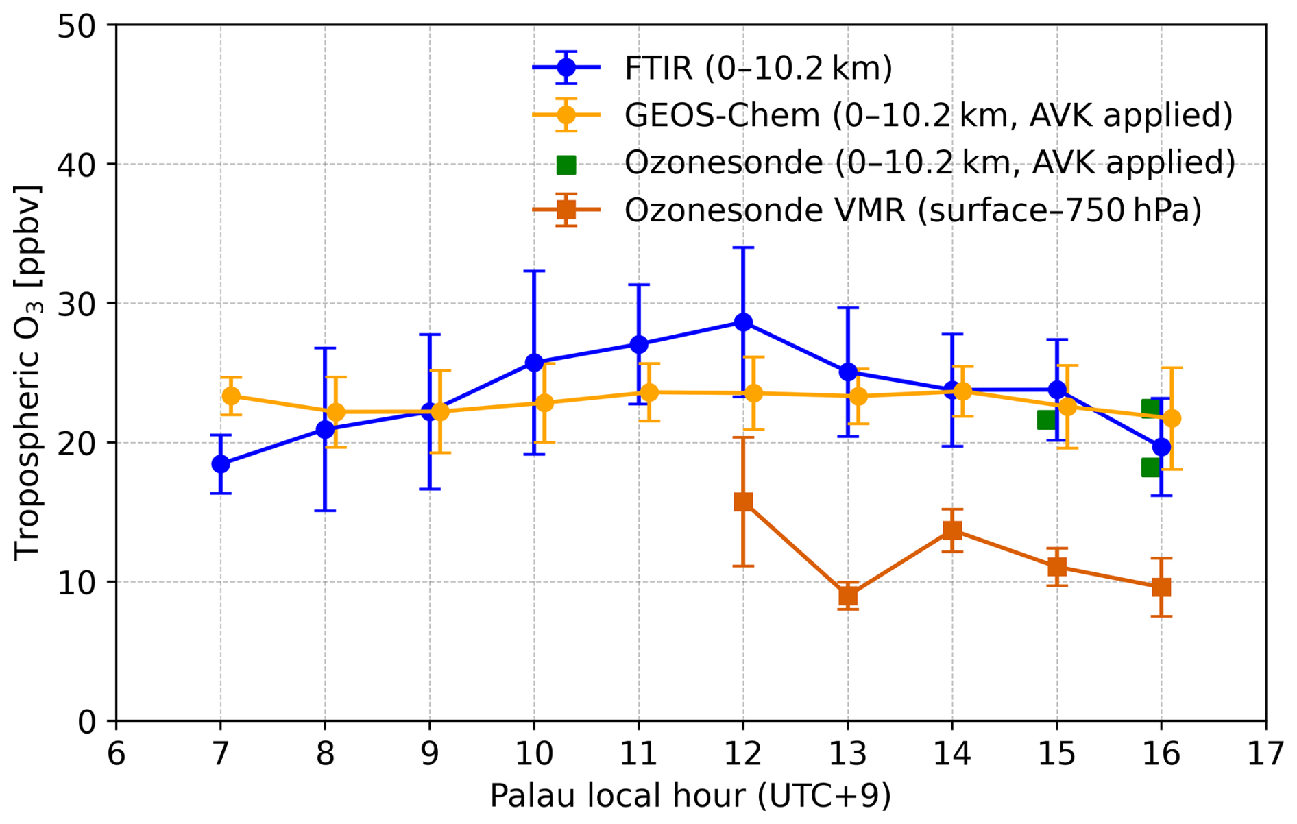
Figure A1 Diurnal variation of tropospheric ozone over Palau derived from FTIR measurements, GEOS-Chem simulations, and ozonesonde observations. Blue circles show FTIR-derived tropospheric ozone (0–10.2 km), orange circles denote GEOS-Chem results smoothed with the FTIR AVK over the same altitude range, and green squares indicate AVK-smoothed ozonesonde tropospheric ozone (0–10.2 km). Orange squares represent ozonesonde volume mixing ratios averaged over the near-surface layer (surface–750 hPa). Error bars denote ±1σ variability. All values are shown as a function of local time (UTC+9).

Table A1 Hourly-binned statistics of FTIR measurements for tropospheric O₃ over Palau.

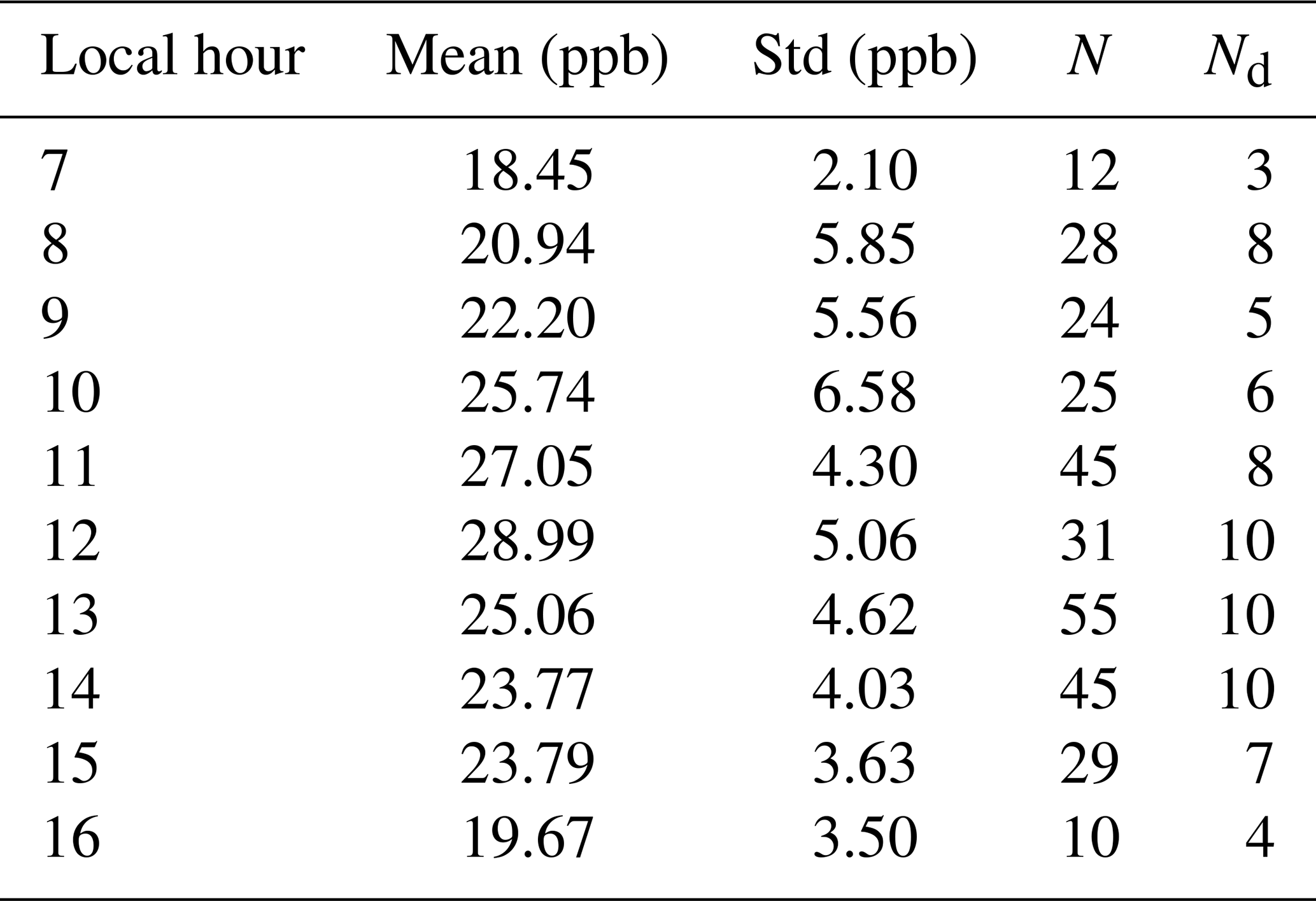
For the FTIR observations, diurnal ozone statistics were constructed by grouping all valid retrievals during September–October 2022 into hourly bins in local time (UTC+9). For each bin, the mean tropospheric ozone (0–10.2 km) and the corresponding standard deviation (±1σ) were calculated. The standard deviation reflects a combination of instrumental retrieval uncertainty and day-to-day atmospheric variability within each hour. As shown in Table A1, most hourly bins contain more than 20 individual FTIR measurements, spanning multiple independent days (N_d≥3 for most daytime hours).

Ozonesonde observations are more sparsely distributed in time and do not cover all local hours. To ensure comparability, ozonesonde profiles were smoothed using the FTIR AVKs prior to integration over 0–10.2 km. In addition, near-surface ozonesonde ozone (surface–750 hPa) is shown separately to illustrate the stronger amplitude of boundary-layer variability. Error bars for ozonesonde data represent the standard deviation within each hourly bin and mainly reflect natural variability and limited sample size rather than instrumental uncertainty.

Despite differences in sampling frequency and vertical sensitivity, the FTIR and ozonesonde observations show consistent diurnal variation pattern during the overlapping hours. The observed diurnal variation in FTIR-derived tropospheric ozone exceeds the typical retrieval uncertainty and remains robust when considering the reported ±1σ variability. Taken together, the number of observations, multi-day sampling, and explicit treatment of uncertainties support the statistical significance of the diurnal ozone features discussed in the main text.

Appendix B: Uncertainty estimation

B1 SZA influence

To assess the potential impact of solar zenith angle (SZA) on the retrieved tropospheric ozone partial column, we examined the partial column averaging kernel (PC AVK) as a function of SZA. PC AVK quantifies the sensitivity of the retrieved partial column to the true ozone profile at each altitude and varies systematically with SZA (Fig. 1b).

To quantify the potential retrieval bias associated with variations in the AVK under different SZA conditions, we performed an upper-limit error estimation. Specifically, we calculated the layerwise maximum differences in the PC AVK across all SZA conditions:

$$\begin{array}{ll}{\displaystyle }\mathrm{\Delta }{\text{PC AVK}}_i& {\displaystyle }=\underset{\mathit{\theta }}{max}\left({\text{PC AVK}}_i\left(\mathit{\theta }\right)\right)\\ \text{(B1)}& {\displaystyle }& {\displaystyle }-\underset{\mathit{\theta }}{min}\left({\text{PC AVK}}_i\left(\mathit{\theta }\right)\right).\end{array}$$

These values represent the maximum possible sensitivity variation for each layer i due to SZA-dependent retrieval characteristics. We then propagated this AVK perturbation into partial column uncertainty using the a priori ozone VMR profile VMR_i and the dry-air column density n_i in each layer from surface to 10.2 km:

$$\begin{array}{}\text{(B2)}& {\displaystyle }{\displaystyle }\mathrm{\Delta }{X}_{{\mathrm{O}}_{\mathrm{3}},p}=\sum _{i=\mathrm{1}}^N\mathrm{\Delta }{\text{PC AVK}}_i\cdot {\text{VMR}}_i\cdot n_i.\end{array}$$

The resulting upper-limit impact on the 0.2–10.2 km tropospheric ozone partial column is estimated to be no more than 1.9 ppb, corresponding to approximately 7.6 % of the typical retrieved partial column (∼25 ppb) over Palau during the study period. This value should be interpreted as a conservative upper-bound estimate, as it is based on the largest AVK variation observed across all SZA conditions. In reality, the actual PC AVK perturbation within a single day is expected to be smaller than the constructed ΔPC AVK profile, since the co-occurrence of maximum SZA-induced changes in all layers is physically unrealistic, see Fig. 1b. In all cases, the impact of AVK variability (1.9 ppb, 7.6 %) in the near-surface layer is smaller relative to the diurnal variation magnitude of approximately 8 ppb, as shown in Fig. 3.

Additionally, Fig. B1 shows the hourly mean ozone concentrations from GEOS-Chem for September–October 2022. The model exhibits no discernible diurnal variation from the surface to the upper troposphere (model levels 992.5–356.3 hPa). Moreover, as shown in Fig. B1, there is a strong relative diurnal variability for OH over Palau. However, the absolute concentrations of OH and NO_x remain extremely low (peak OH<0.5 ppt; NO_x<40 ppt). Under such pristine, NO_x-limited conditions, the absolute photochemical turnover (the net rate of ozone production and loss) is very small. Therefore, even significant relative fluctuations in radical abundance do not translate into a pronounced diurnal cycle in the total ozone column. The inability of the model to capture the observed afternoon ozone peak suggests that localized O₃ production or vertical transport processes may be smoothed out by grid resolution of the model. For a consistent comparison with the FTIR observations, the model profiles were smoothed using the FTIR AVK. Nevertheless, even after AVK smoothing the modeled ozone diurnal cycle remains much weaker than observed (Fig. 3a). This demonstrates that the inability of GEOS-Chem to reproduce the observed diurnal ozone cycle cannot be attributed to AVK smoothing or retrieval artifacts, but instead reflects insufficient diurnal variability in the modeled chemical and dynamical processes.

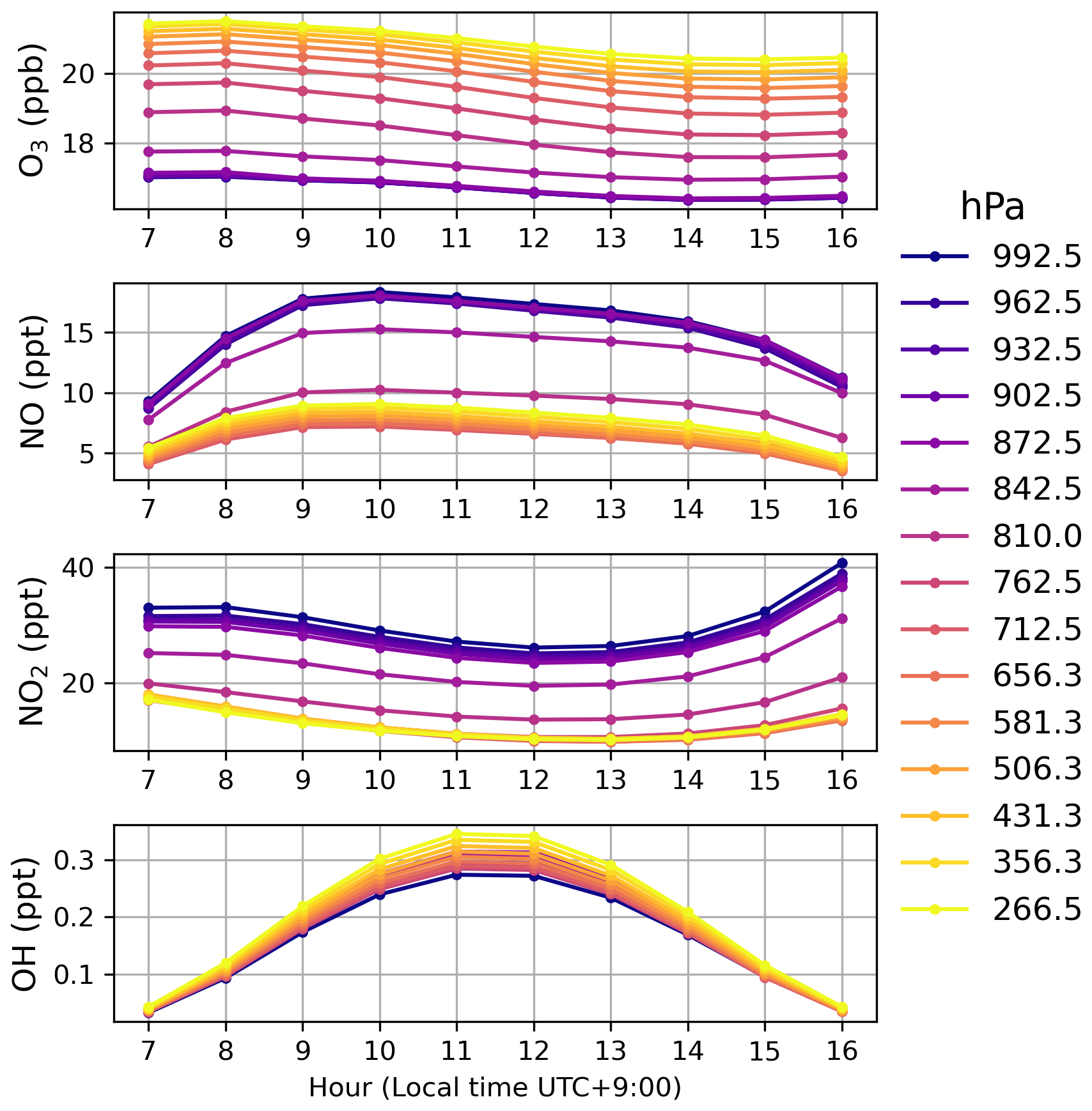
Figure B1 Hourly mean O₃, NO, NO₂, and OH concentrations from GEOS-Chem simulations for September–October 2022, shown at individual model levels (992.5–356.3 hPa).

B2 Stratosphere effect in the tropospheric O₃ column

To evaluate potential overestimation of tropospheric ozone due to the vertical sensitivity of the retrieval, we analyzed the impact of AVK tails above the target range (0–10.2 km), see Fig. 1a. Unlike trace gases such as CO or CH₄, whose concentrations decrease with altitude, ozone concentrations increase rapidly near the tropopause and into the lower stratosphere. As a result, even moderate AVK values above 10 km (ranging from ∼0.5 to 0.0 between 10–20 km) can lead to a measurable contribution to the retrieved partial column.

To estimate this “leakage” effect from upper level especially for stratospheric ozone, we applied the AVK vector for the first degree of freedom (DOF=1) to the a priori ozone profile and computed the portion of the column originating from altitudes above 10.2 km:

$$\begin{array}{ll}{\displaystyle }{\text{VMR}}_{\text{leak}}^{\text{dry air},p}& {\displaystyle }={\displaystyle \frac{\mathrm{1}}{{\text{PC}}^{\text{dry air},p}}}\sum _{z>\mathrm{10.2}\text{km}}{\text{VMR}}_{\text{ap}}\left(z\right)\cdot \text{AVK}\left(z\right)\\ \text{(B3)}& {\displaystyle }& {\displaystyle }\cdot \mathrm{\Delta }{\text{PC}}^{\text{dry air}}\left(z\right).\end{array}$$

Here, ΔPC^{dry air}(z) denotes the dry air partial column in each layer, and PC^{dry air,p} is the total dry air column within the retrieval's first partial column layer (0–10.2 km). This provides an equivalent ozone mixing ratio resulting from high-altitude leakage. The estimated leakage error is approximately 1.5 ppb, corresponding to 6 % of the typical tropospheric ozone column (∼25 ppb) during the measurement period. So we use this value to assign a 6 % uncertainty for the stratosphere effect, suggesting that a small fraction of stratospheric ozone is aliased into the tropospheric partial column. Rather than undermining the retrieval, this reinforces our conclusion that ozone over Palau is exceptionally low – possibly even lower than the retrieved values. Comparisons with coincident radiosonde observations support this finding and confirm that the leakage remains within the expected uncertainty range.

This method offers a simplified estimate of vertical smoothing error, consistent with the principle introduced by Rodgers (2000) and von Clarmann (2014). This estimation method follows the principles of these two methodologies and evaluates the impact of the average nuclear tail on the inversion value by applying AVK to the reference profile. Although we use a prior profile rather than the actual state, this method can still provide a preliminary estimate of the vertical smoothing effect (i.e. upper layer leakage AVK), which is important for partial column inversion, especially for species like O₃ with higher VMR at higher altitudes.

B3 Estimation of near-surface contribution to tropospheric column ozone

The TOC retrieved from FTIR represents the vertically averaged dry-air column mole fractions response to the surface ozone variability. When most of the diurnal variability is confined to the near-surface layer and the free troposphere remains relatively constant, the integration and averaging dampen the observed signal. To quantify this damping, we define a ratio T between the peak-to-peak amplitude of the TOC and that of the near-surface layer, using the partial PC AVK of the FTIR retrievals:

$$\begin{array}{}\text{(B4)}& {\displaystyle }& {\displaystyle }{T}_{\text{avk}}={\displaystyle \frac{\mathrm{1}}{\langle a{\rangle }_{z_{\mathrm{0}}-\mathrm{\Delta }{z}_{\text{BL}}}}}{\displaystyle \frac{{\int }_{z_{\mathrm{0}}}^{z_{\mathrm{10}}}\text{AVK}\left(z\right)a\left(z\right)\mathrm{d}z}{{\int }_{z_{\mathrm{0}}}^{z_{\mathrm{10}}}\text{AVK}\left(z\right)\mathrm{d}z}},\text{(B5)}& {\displaystyle }& {\displaystyle }\langle a{\rangle }_{z_{\mathrm{0}}-\mathrm{\Delta }{z}_{\text{BL}}}={\displaystyle \frac{\mathrm{1}}{\mathrm{\Delta }{z}_{\text{BL}}}}\underset{z_{\mathrm{0}}}{\overset{z_{\mathrm{0}}+\mathrm{\Delta }{z}_{\text{BL}}}{\int }}a\left(z\right)\mathrm{d}z.\end{array}$$

Here, T represents the fraction of near-surface variability that is visible in the TOC. AVK(z) is the FTIR partial column averaging kernel corresponding to the retrieved tropospheric column (0–10.2 km). a(z) is a linear decay shape function for the diurnal amplitude, which is derived from the near-surface ozone gradients reported by Petetin et al. (2016), assuming a linear decrease from the surface to 2.5 km (see details below). The term $\langle a{\rangle }_{z_{\mathrm{0}}-\mathrm{\Delta }{z}_{\text{BL}}}$ denotes the mean amplitude within the near-surface layer of thickness, where discernible O₃ variability is observed Δz_BL (Petetin et al., 2016). In this study, we set Δz_BL=2.5 km, corresponding approximately to 750 hPa at Palau based on ozonesonde profiles. Applying this method to all available FTIR PC AVKs yields a median T value of 0.4, indicating that the TOC captures about 40 % of the near-surface diurnal ozone variability. This factor quantifies the damping introduced by column integration and the retrieval sensitivity.

The above estimate is based on an idealized vertical shape function a(z) that linearly decreases from the surface to zero at Δz_BL=2.5 km. To assess the robustness of this approach, we tested alternative profiles, including exponential decays with scale heights of 0.6–1.0 km, and stepwise reductions following the boundary layer evolution reported by Petetin et al. (2016). Across these scenarios, the resulting T values varied within 0.35–0.45, consistent with the median value of 0.4 reported above.

In addition, we considered the dependence of the PC AVK on SZA. The overestimation of the ozone diurnal cycle by the SZA effect of 1.9 ppb (Appendix B1), the 8 ppb peak-to-peak diurnal amplitude during the campaign (Fig. 3 in Sect. 3.1) can be estimated to 6 ppb. Then, we estimated that the peak-to-peak diurnal magnitude of the near-surface ozone is about 15 ppb. Therefore, the conclusion that the FTIR tropospheric ozone column captures approximately 40 % of the near-surface diurnal variability is robust against reasonable assumptions about the vertical amplitude shape and SZA-dependent retrieval sensitivity of approximately 7.6 %.

Appendix C: Sensitivity test results

Sensitivity studies have been conducted for the Lightning emission over the TWP region. Figure C1 shows the Tropospheric O₃, OH, and NO simulated by GEOS-Chem and averaged over the study period. The difference between the sensitivity study and the base simulation is shown in Fig. 6. Note that the color bar scale is larger than the variation in NO; the difference between Fig. C1 is not visible, especially at very low NO values over the TWP region.

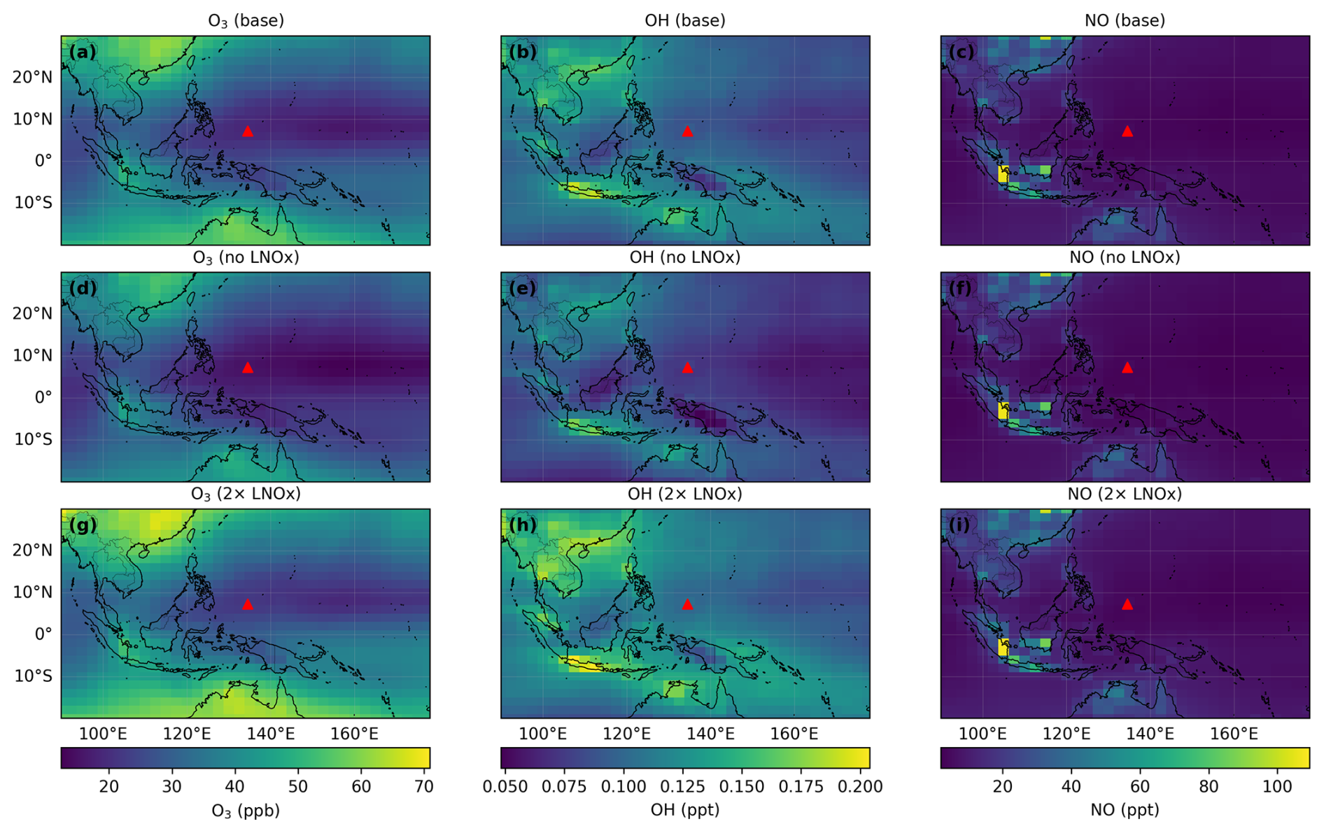
Figure C1 Tropospheric ozone (O₃), hydroxyl radical (OH), and nitric oxide (NO) columns simulated by GEOS-Chem and averaged over the study period. (a–c) The base simulation with LNO_x emissions included. (d–f) The sensitivity simulation with LNO_x emissions turned off (no NO_x), and (g–i) the simulation with doubled LNO_x emissions (2×NO_x). Columns correspond to O₃, OH, and NO from left to right. The red triangle marks the location of the Palau FTIR measurement site.