Natural and anthropogenic influence on tropospheric ozone variability over the Tropical Atlantic unveiled by satellite, reanalyses and in situ observations

Tropospheric ozone over the South and Tropical Atlantic plays an important role in the photochemistry and energy budget of the atmosphere. In this remote region, tropospheric ozone estimates from reanalysis datasets show the largest discrepancies. The present study characterises the vertical and horizontal distribution of tropospheric ozone over the South and Tropical Atlantic during February and October 2017 using a multispectral synergism called IASI + GOME2, two global chemistry reanalysis products – the Copernicus Atmosphere Monitoring Service reanalysis (CAMS reanalysis) and the Tropospheric Chemistry Reanalysis version 2 (TCR-2) – and in situ airborne measurements from the Atmospheric Tomography Mission (ATom). In February, biomass burning in West and Central Africa and deep convection over the Gulf of Guinea strongly influence the region. IASI + GOME2 captures enhanced ozone abundances in the Southern Hemisphere and low ozone concentrations in the Northern Hemisphere, exhibiting excellent agreement with ATom-2 profiles. In contrast, both reanalyses underestimate lower-tropospheric ozone influenced by biomass-burning outflow and overestimate ozone in the Northern Hemisphere due to excessive contributions from stratospheric intrusion and North American anthropogenic emissions. In October, tropospheric ozone enhancement associated with biomass-burning outflow from Austral Africa is consistently depicted by observations and reanalyses. These results emphasize the need to evaluate the seasonal variability of each of the multiple sources of ozone precursors within atmospheric chemistry reanalyses.

1 Introduction

Tropospheric ozone is one of the key gases in the atmosphere because it is a major greenhouse gas (Szopa et al., 2021) and it plays an important role in determining the oxidising capacity of the troposphere (Monks et al., 2015). The main source of tropospheric ozone is in situ photochemical production via oxidation of non-methane volatile organic compounds (NMVOCs), carbon monoxide (CO), and methane (CH₄), in the presence of nitrogen oxides (NO_x) (e.g., Atkinson, 2000). These ozone precursors originate from both anthropogenic (fossil fuel combustion in power plants, industrial activities, transportation and crop burning) and natural sources (wetland CH₄ emissions, wildfires, biogenic hydrocarbon emissions, lightning and soil NO_x emissions) (e.g., Elshorbany et al., 2024). The abundance of tropospheric ozone is also controlled by transport from the ozone-rich stratosphere. The net influx ozone from the stratosphere was estimated at 552±168 Tg, and is smaller than the amount of chemical production (5110±606 Tg; Young et al., 2013). The lifetime of ozone in the troposphere ranges from a few hours in polluted urban areas to up to a few weeks in the free troposphere, but is relatively long on average (∼22 d; Young et al., 2013). This allows tropospheric ozone to be transported over distances of intercontinental and hemispheric scales.

By increasing computing performance and availability of satellite observations of trace gases, data assimilation has been applied with success in monitoring air quality (e.g., Flemming et al., 2015; Gelaro et al., 2017; Inness et al., 2019; Miyazaki et al., 2015, 2020). Data assimilation is a methodology that allows a physical-chemically based interpolation to fill in of the observational information gaps using a model and to provide an estimate of the most likely state and its uncertainty. Applications of data assimilation to atmospheric chemistry can improve analyses of tropospheric pollution, and can provide estimates of tropospheric emissions (Lahoz and Schneider, 2014). The result of data assimilation is termed a “reanalysis” when the data assimilation approach is performed for past data by using a consistent system. Atmospheric chemistry reanalysis products have been produced using multi-species satellite observations. There have been several studies that compared atmospheric chemistry reanalysis products. Air pollutants including ozone and CO derived from some chemistry reanalysis products were evaluated on regional scale in East Asia (Park et al., 2020; Ryu and Min, 2021; Zhang et al., 2022) and Europe (Falk et al., 2021; Lacima et al., 2023). Huijnen et al. (2020) intercompared four atmospheric chemistry reanalysis products and reported that the standard deviation (SD) is the largest over South America, the Tropical Atlantic and Central Africa because of their differences of the representations of biomass-burning emissions and its impacts on ozone production, the representation of convective transport, and large uncertainties in biogenic emissions.

The South and Tropical Atlantic has been a region of intense interest in the ozone scientific community since Fishman and Larsen (1987) identified a regional maximum in tropospheric ozone derived from satellite measurements. This discovery was the motivation for a large-scale ground and aircraft study in the southern biomass burning season in September and October 1992: IGAC/STARE/SAFARI-92/TRACE-A (International Global Atmospheric Chemistry/South Tropical Atlantic Regional Experiment/Southern African Fire Atmospheric Research Initiative/Transport and Atmospheric Chemistry near the Equator-Atlantic). SAFARI-92/TRACE-A confirmed the regional ozone feature with aircraft profiling and lidar plus ozonesondes deployed over Brazil, Ascension Island and three sites in sub-Saharan Africa. In addition, analyses of the comprehensive SAFARI-92/TRACE-A data confirmed links of the Atlantic maximum to fire activity over Africa (Fishman et al., 1996; Thompson et al., 1996) and to ozone formed from a combination of fires, deep convection and lightning activity over South America (Pickering et al., 1996). Based on ozonesonde profiles, it was estimated that the relative contributions to the Atlantic ozone were approximately two-third from African sources and one-third from South America (Thompson et al., 1996). However, dynamic influences were required for the ozone hotspot to form. Krishnamurti et al. (1996) demonstrated that recirculation within the South Atlantic gyre allowed the ozone to accumulate so that the highest ozone amounts were found over the ocean rather than the continents.

Shipboard ozone sampling over the Tropical Atlantic provided additional insights into South Tropical Atlantic ozone (Thompson et al., 2000; Weller et al., 1996). These measurements suggested that the ozone maximum occurs at all seasons, not only during the peak of Southern Hemisphere burning but also when African fire activity is at its greatest north of the Inter-Tropical Convergence Zone (ITCZ). This so-called “Atlantic ozone paradox” was associated with upper tropospheric-stratospheric subsidence and lightning in addition to fires (Thompson et al., 2000). These contributions were evaluated in an early model study (Moxim and Levy, 2000). The SAFARI-92/TRACE-A experiments were instrumental in assembling the Southern Hemisphere Additional Ozonesondes (SHADOZ) network of stations that has operated from 1998 to the present day (Thompson et al., 2017). With coordinated launches of ozonesondes from more than 10 stations across the tropics, the Atlantic maximum is a strong feature with the South Tropical Atlantic always exhibiting more tropospheric column ozone (5–15 Dobson Units, 1 DU = 2.69×10¹⁶ cm⁻²). When looking at the tropospheric ozone structure across the entire tropical band, the Atlantic ozone feature leads to a zonal wave one pattern (Thompson et al., 2003).

More recently, additional studies of the role of biomass burning (van der Werf et al., 2017), biogenic sources (Sindelarova et al., 2022) and lightning (Schumann and Huntrieser, 2007) contributions to Atlantic, African and South American ozone has been conducted. Among other features, they estimate that lightning is the major driver of the dominating ozone sensitivity in the upper tropical troposphere (Nussbaumer et al., 2023; Schumann and Huntrieser, 2007). Additional analyses of tropical ozone distributions (mostly in the upper troposphere) were performed using in situ measurements onboard commercial aircrafts (Lannuque et al., 2021; Sauvage et al., 2005, 2007b; Tsivlidou et al., 2023; Yamasoe et al., 2015). This is the case of the In-Service Aircraft for a Global Observing System (IAGOS) European Research Infrastructure (e.g., Petzold et al., 2015), the former research projects the Measurement of Ozone and Water Vapour on Airbus In-service Aircraft (MOZAIC) and the Civil Aircraft for the Regular Investigation of the Atmosphere Based on an Instrument Container (CARIBIC). Their results show for example that lightning has the largest influence on the South Atlantic ozone burden (24° S–0°, 35° W–10° E), accounting for more than 37 % (Sauvage et al., 2007a). The authors quantified that the contributions of biomass burning, fossil fuel combustion, and soil NO_x emissions to the tropospheric ozone column were 6, 5, and 4 times smaller than that from lightning. In addition, the Tropical Atlantic ozone burden was more strongly influenced by NO_x from Africa than from South America. Trends in tropical tropospheric ozone have been reported using SHADOZ ozonesonde profiles (Thompson et al., 2021) and a combination of satellite, SHADOZ and IAGOS aircraft measurements (Gaudel et al., 2024). However, most of IAGOS data is acquired in the extratropical upper troposphere/lower stratosphere (UTLS) and in the tropical upper troposphere when the aircraft attain cruising altitude in the altitude band of 9–13 km (see Sect. S1 and Fig. S1 in the Supplement). Thus, the ozone regional distribution in the middle and lower troposphere over the South and Tropical Atlantic is much less documented.

Satellite observations offer a great potential to overcome the limited spatial coverage of ground-based measurements. However, standard single-band ozone retrievals are not able to provide quantitative measurements of ozone abundance within the planetary boundary layer. Ultraviolet (UV) spaceborne spectrometers, like GOME-2 (Global Ozone Monitoring Experiment-2), have been used to observe tropospheric ozone with maximum sensitivity at about 5–6 km altitude (e.g., Liu et al., 2010; Cai et al., 2012). Space-based thermal infrared (TIR) instruments, such as the Infrared Atmospheric Sounding Interferometer (IASI) on board the MetOp satellites, have shown good performance for observing ozone in the lower troposphere but with sensitivity peaking at lowest at 3 km altitude (e.g., Eremenko et al., 2008; Dufour et al., 2012). More recently, synergetic approaches using UV and TIR radiances simultaneously have been developed to improve the sensitivity to lower tropospheric ozone (e.g., Cuesta et al., 2013; Fu et al., 2018; Colombi et al., 2021). These multispectral methods are different from merging different satellite products, as all information on ozone vertical distribution is extracted from measurements of different spectral domains at once into a single ozone product. The multispectral synergism called IASI + GOME2, combining IASI observations in the TIR and GOME-2 measurements in the UV, shows remarkable skills in observing the horizontal distribution of ozone concentrations in the lowermost troposphere (LMT – here after defined as the atmospheric partial column below 3 km of altitude, Cuesta et al., 2013). Air-quality-relevant capabilities of IASI + GOME2 have been demonstrated by quantitatively describing the transport pathways, the daily evolution, and photochemical production in the lowermost troposphere during transboundary ozone pollution events across east Asia (Cuesta et al., 2018) and Europe (Cuesta et al., 2013, 2022; Okamoto et al., 2023). Atmospheric chemistry reanalysis products are assimilated by a variety of satellite observations (mostly total and tropospheric columns) and helps better understandings of spatiotemporal variability and long-term trends. It is crucial to characterize the strengths and limitations of the reanalysis products, in particular at the surface and in the lower troposphere, as no in situ observations are assimilated.

The paper aims to describe the tropospheric ozone variability over the South and Tropical Atlantic in two seasons of 2017 extracting the best of three datasets: IASI + GOME2 satellite measurements and two global chemistry reanalyses. We use in situ measurements performed by a research aircraft within the Atmospheric Tomography Mission (ATom) in February and October 2017, for their high accuracy (thus providing a reference) and the availability of measurements of multiple chemical tracers for understanding the origins of the air masses with high and low abundances of tropospheric ozone. This last highly valuable dataset remains representative of only local to regional scales, limited to the track of the aircraft. IASI + GOME2 satellite data is a key and new observational dataset, providing a unique 3D observation of the tropospheric ozone distribution from regional to large scale, generalizing at larger spatial and temporal scale what is described more locally by ATom and whose good match provides confidence with good representativity. Reanalysis products are used to describe the ozone distribution together with those of its precursors as a key wrapping up elements of the study. The use of three datasets also allows an intercomparison which is additional useful to highlight the strengths and limitations of the satellite datasets and the reanalyses, with in situ measurements as reference. Section 2 describes the satellite data, atmospheric chemistry reanalysis products and in situ observations used for the analysis. Results and discussions on the distribution of tropospheric ozone and CO over the Tropical and South Atlantic are presented in Sect. 3. Conclusions are given in the last section (Sect. 4).

2 Data and methods

In this study, we characterize the tropospheric ozone distribution over the Tropical Atlantic using data from a satellite approach and two chemistry reanalysis products. To analyse the origin of ozone plumes, CO satellite retrievals and two chemistry reanalysis products are also employed. We consider the region covering the Atlantic Ocean between 40° S and 40° N to investigate interactions of pollution and the transport between the tropics and the subtropics. This section provides and overview of the datasets used in this study, including satellite data (Sect. 2.1), atmospheric chemistry reanalyses (Sect. 2.2), in situ airborne measurements (Sect. 2.3), meteorological data (Sect. 2.4) and other data (Sect. 2.5).

2.1 Satellite data

2.1.1 IASI + GOME2 ozone multispectral synergism

The IASI + GOME2 multispectral synergism is designed for observing lowermost tropospheric ozone by synergism of TIR atmospheric radiances observed by IASI and UV earth reflectances measured by GOME-2 (Cuesta et al., 2013, 2018). Both instruments are onboard the MetOp satellite series. MetOp-B (in orbit since 2006) offers global coverage every day with a relatively fine ground resolution (12 km diameter pixels spaced by 25 km for IASI at nadir and ground pixels of 80 km × 40 km for GOME-2). The MetOp-B has an Equator crossing time of 09:30 LT (local time) in the descending node. Spectra and Jacobians in the IR and UV are simulated by the KOPRA (Karlsruhe Optimized and Precise Radiative transfer Algorithm; Stiller et al., 2002) and VLIDORT (Vector Linearized Discrete Ordinate Radiative Transfer; Spurr, 2006) radiative transfer codes, respectively. Ozone profiles are retrieved on a vertical grid between the surface and 60 km of altitude. The IASI + GOME2/MetOp-B ozone product including vertical profiles of ozone, averaging kernel, error estimations and quality flags is provided by the French data centre AERIS (https://iasi.aeris-data.fr, last access: October 2023). For reducing random errors, the product is averaged over a regular horizontal grid of 1° × 1°, in the same way as done by Cuesta et al. (2018). Ozone concentrations are provided as an average ozone volume mixing ratio in ppb within the column, which is calculated from the ratio of each partial column of ozone and air.

2.1.2 IASI carbon monoxide retrievals

The CO retrievals used in this study are derived from IASI radiances using the FORLI algorithm (Fast Optimal Retrievals on Layers for IASI; Hurtmans et al., 2012), from the Université Libre de Bruxelles (ULB) and the Laboratoire Atmosphères, Milieux, Observations Spatiales (LATMOS). This approach uses pre-calculated lookup tables of absorbance cross sections at various pressures and temperatures, and an optimal estimation method for the inverse scheme. The algorithm derives vertical profiles of CO, on a grid of 18 equidistant layers of 1 km of depth from the surface up to 18 km, and a unique layer from 18 to 60 km. The IASI/MetOp-B CO product including total and partial columns of CO derived by profile integrations, averaging kernels, error estimations and quality flags is provided by the French data centre AERIS (https://iasi.aeris-data.fr, last access: November 2024). The product is averaged over a regular horizontal grid of 1° × 1° and CO concentrations are calculated from average CO volume mixing ratio in ppb within the column in the same way as far IASI + GOME2 ozone.

2.2 Atmospheric chemistry reanalyses

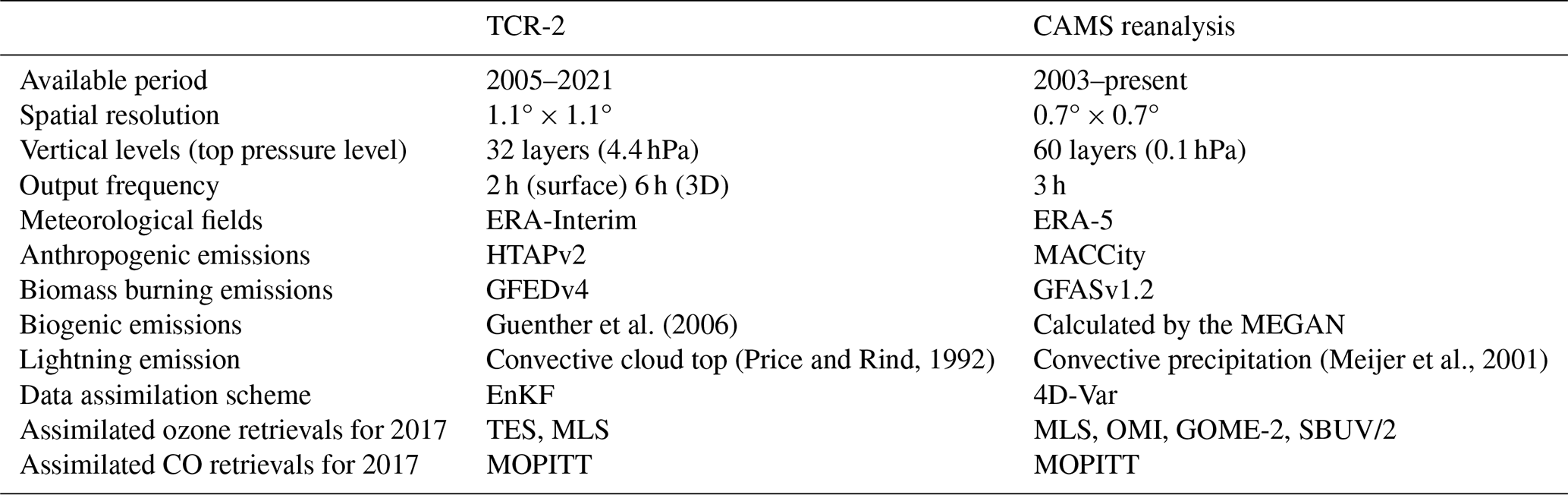
The global atmospheric chemistry reanalysis products compared in this paper are the Tropospheric Chemistry Reanalysis version 2 (TCR-2) and the Copernicus Atmosphere Monitoring Service reanalysis (CAMS reanalysis) and are listed in Table 1. The general configuration of the various data assimilation systems is provided in the following subsections. We regrid these atmospheric chemistry reanalysis products to 1° × 1° resolutions for consistency with gridded IASI + GOME2 ozone data. Then, we convert their pressure levels to altitude by using geopotential fields from ERA5 (Sect. 2.4).

Table 1 Overview of the global atmospheric chemistry reanalysis products.

2.2.1 Tropospheric Chemistry Reanalysis version 2 (TCR-2)

TCR-2 (Miyazaki et al., 2019) is a global atmospheric chemistry reanalysis based on the MIROC-CHASER (Model for Interdisciplinary Research on Climate-Chemical atmospheric general circulation model for study of atmospheric environment and radiative forcing, Watanabe et al., 2011) by the National Aeronautics and Space Administration (NASA) Jet Propulsion Laboratory (JPL) (Miyazaki et al., 2020). TCR-2 uses an ensemble Kalman filter (EnKF) data assimilation technique to combine satellite observations of ozone, CO, nitrogen dioxide (NO₂), nitric acid (HNO₃) and sulphur dioxide (SO₂). TCR-2 has a T106 horizontal resolution (0.7° × 0.7°) with 32 vertical levels from surface to 4.4 hPa. TCR-2 is available at 2 h intervals for surface concentrations and at 6 h intervals for 3-D concentrations. Meteorological fields used by TCR-2 are nudged towards the 6-hourly ERA-Interim (Dee et al., 2011). A priori surface emissions from anthropogenic sources are obtained from the HTAP version 2 for 2010 (Janssens-Maenhout et al., 2015). For biomass burning emissions, the monthly Global Fire Emissions Database (GFED) version 4 (Randerson et al., 2018) is used. Emissions from soils are based on monthly mean Global Emissions Inventory Activity (GEIA) (Yienger and Levy, 1995). Biogenic emissions from vegetation are considered for non-methane hydrocarbons (NMHCs) based on Guenther et al. (2006). Lightning NO_x (LNO_x) sources were simulated by using the convection scheme of MIROC-AGCM (Miyazaki et al., 2017). The global distribution of the flash rate was parameterized for convective clouds based on the relationship between lighting activity and cloud top height (Price and Rind, 1992). The vertical profile of the LNO_x sources were determined on the basis of the C-shape profile, which peaks at the surface and in the upper troposphere, given by Pickering et al. (1998). In the present study, we use 2-hourly ozone and CO TCR-2 data (Kazuyuki Miyazaki, personal communication, 2020).

2.2.2 Copernicus Atmosphere Monitoring Service reanalysis (CAMS reanalysis)

CAMS reanalysis is a global atmospheric chemistry reanalysis based on the Integrated Forecast System (IFS) cycle 42R1 by the European Centre for Medium-Range Weather Forecasts (ECMWF) (Inness et al., 2019, last access: 12 April 2022). CAMS reanalysis uses the four-dimensional variational (4D-Var) data assimilation technique to combine satellite observations of ozone, CO, NO₂ and aerosol optical depth (AOD). The spatial resolution of CAMS reanalysis is a reduced Gaussian grid at a spectral truncation of T255, which is equivalent to grid spacing of approximately 80 km globally (0.7° × 0.7°), with 60 vertical levels from surface to 0.1 hPa. CAMS reanalysis is available at 3 h intervals. Daily global biomass burning emissions are provided by the Global Fire Assimilation System (GFAS) version 1.2 (Kaiser et al., 2012). Anthropogenic emissions are from the MACCity inventory (Granier et al., 2011), with modifications to increase wintertime road traffic emissions over North America and Europe following the correction of Stein et al. (2014). Monthly mean biogenic emissions are calculated offline by the Model of Emissions of Gases and Aerosols from Nature (MEGAN, Guenther et al., 2006) that used meteorological fields from the Modern-Era Retrospective analysis for Research and Applications version 2 (MERRA-2) following Sindelarova et al. (2014). Natural emissions from soils and oceans are taken from the “Precursors of Ozone and their Effects in the Troposphere” (POET) database (Granier et al., 2005; Olivier et al., 2003). LNO_x emissions are simulated by the modules for atmospheric composition in the IFS, named Composition-IFS (C-IFS) (Flemming et al., 2015). In the IFS, LNO_x emissions uses the parameterisation of Meijer et al. (2001) based on convective precipitation. The smaller land–sea differences of Meijer et al. (2001) agreed better with the observations. The observed maximum over central Africa was well reproduced by both parameterisations (convective cloud top and convective precipitation), while an exaggerated maximum was remarked over tropical South America. The vertical profile of the LNO_x sources were determined on the basis of the backward C-shape profile, which locates most emission in the middle of the troposphere, given by Ott et al. (2010).

2.3 The Atmospheric Tomography Mission (ATom)

The Atmospheric Tomography Mission (ATom) is a NASA Earth Venture airborne field campaign to study the impacts of human-produced air pollution on greenhouse gases and on chemically reactive gases over the Pacific and Atlantic oceans along a global-scale circuit (Thompson et al., 2022). ATom consists of four series of flights from ∼82° N to ∼86° S by using the long-range NASA DC-8 research aircraft. During these flights, the DC-8 repeatedly ascended and descended between ∼0.2 and ∼13 km in altitude. The four ATom circuits occurred in July–August 2016 (ATom-1), January–February 2017 (ATom-2), September–October 2017 (ATom-3), and April–May 2018 (ATom-4).

The ATom dataset includes merged data from all instruments (Wofsy et al., 2018) provided by the Oak Ridge National Laboratory Distributed Active Archive Center (ORNL DAAC, last access: 24 March 2023). We use ozone and CO observations to compare with satellite and reanalysis products. In addition, we use water vapor (H₂O), hydrogen cyanide (HCN, biomass burning tracer), tetra chloroethylene (C₂Cl₄, urban tracer) and NO_x observations to quantify the influences of biomass burning and urban emissions. The measurement methods of these tracers are described in detail elsewhere (Bourgeois et al., 2021). We classify air masses into six types (stratospheric air, marine air, urban air, biomass burning air, mixed pollution air, and well-mixed and aged air) based on the method of Bourgeois et al. (2021) (Sect. S2 in the Supplement).

A dataset containing back trajectories and boundary layer influences of air parcels along the ATom flight tracks is also provided by the ORNL DAAC NASA's data centre (Ray, 2021, last access 22 December 2023). We use these two products, that are driven by National Centers for Environmental Prediction (NCEP) Global Forecast System (GFS) meteorology. They are calculated by initialising model trajectories at receptors spaced 1 min apart along the ATom flight tracks, followed backwards for 30 d, and reported at 3 h resolution. We also use average probability of boundary layer influence in the dataset to identify air masses influenced by lightning (Sect. 3.3). The boundary layer influences product provided by ORNL DAAC is determined based on the location of these air masses along 30 d back trajectories.

2.4 Meteorological data

Meteorological conditions leading to photochemical production of ozone and transport are described with the ERA5 reanalysis (Hersbach et al., 2020) produced by the European Centre for Medium-Range Weather Forecast (ECMWF). We use meteorological fields with global coverage, a horizontal resolution of 0.25° × 0.25°, 37 pressure levels, and a time step of 1 h. Eastward and northward components of wind, vertical velocity, relative humidity, geopotential, and potential vorticity are used to describe transport patterns downloaded from the Climate Data Store (https://cds.climate.copernicus.eu/, last access: 19 December 2023).

The NO_x production by lightning is generally represented by parameterizations in global chemistry transport models, resulting in uncertainties put in evidence by differences between models. The World Wide Lightning Location Network (WWLLN) is a global network monitoring lightning activity by very low frequency radio sensors (Dowden et al., 2002). Recently, a global, high-resolution gridded time series and climatology of lightning stroke density, the WWLLN Global Lightning Climatology (WGLC) has been published (Kaplan and Lau, 2021) and is freely available at 0.5° and 5 arcmin spatial resolution and with daily and monthly temporal resolution (Kaplan and Lau, 2022, last access: 19 April 2023). Details are given in Sect. S3 in the Supplement.

As a convective proxy, we use monthly outgoing longwave radiation (OLR) data distributed by the National Oceanic and Atmospheric Administration (NOAA) Physical Science Laboratory (PSL) (Liebmann and Smith, 1996; https://psl.noaa.gov/, last access: 10 March 2023). The OLR is a good indicator of the position of the ITCZ. Deep convective clouds present at the ITCZ are associated with OLR below 220 W m⁻² (e.g. Park et al., 2007).

2.5 Other data

The locations of fires are derived from the Terra and Aqua MODIS (Moderate Resolution Imaging Spectrometer) active fire products (MCD14ML Collection 6; Giglio et al., 2016) distributed by the Fire Information for Resources Management System (FIRMS; https://firms.modaps.eosdis.nasa.gov/, last access: 13 March 2020). This dataset provides the values of fire radiative power (FRP) and the inferred hotspot type: “presumed vegetation fire”, “active volcano”, “other static land source”, and “offshore”. We only use the FRP values of presumed vegetation fire with a confidence level greater than 50 %.

3 Results and discussion

The analysis of the distribution and origins of tropospheric ozone over the Tropical Atlantic is presented here in two steps. First, in Sect. 3.1, we analyse the monthly evolution of key processes that influence ozone distribution, namely tropical convective activity described by lightning and biomass burning emissions estimated by fire detections. We also quantify the differences between several tropospheric ozone products (from models and satellite observations) to identify the period with the largest uncertainties. This leads to a more detailed description of the tropospheric ozone distribution in one of the months with the largest uncertainties (February) and in one of the months with the smallest uncertainties (October).

The following Sect. 3.2 looks in detail at the distribution of tropospheric ozone and carbon monoxide, an ozone precursor derived from combustion and thus used to identify the air mass origin of either biomass fires or anthropogenic activities. This section is followed by a detailed description of the origins of tropospheric ozone and its precursors (Sect. 3.3), and vertical profiles of tropospheric ozone and CO including an explanation of the gaps between observational (both in situ and satellite) and modelling (atmospheric chemistry reanalysis) data sets (Sect. 3.3 and 3.4). This is done with coincident ATom in situ observations, satellite measurements and reanalysis during the periods 13–15 February and 17–20 October 2017.

3.1 Monthly evolution of tropospheric ozone and related variables over the Tropical Atlantic

Climate in the tropics is characterised by alternating wet and dry seasons depending on the position of the ITCZ (Nicholson, 2018). The ITCZ moves north in the Northern Hemisphere summer and south in the Northern Hemisphere winter. Vigorous convection within ITCZ clouds results in charge separation and thunderstorms (Ávila et al., 2010). Lannuque et al. (2021) defined two main seasons (from December to March and from June to October) and two transition seasons (from April to May and November) in the African inter-tropical zone based on the position of ITCZ, defined by zonal and meridional winds and relative humidity because the classical four seasons were not adapted to their study area. In general, the African fire pattern was strongly associated with the movement of the ITCZ over the region (Swap et al., 2002). The peak of burning events over Africa north of the equator occurs in January, whilst south of it in July (Roberts et al., 2009). May and October are expected to be the periods of transition between hemispheres. Over South America, biomass burning emissions start increasing in June, enhance in July and August, and peak in September, and start decreasing in October (Pereira et al., 2022). Details of seasonal variations of lightning and fire activities in 2017 are described in Sect. S4 in the Supplement.

There are strong seasonal variations in the location of fires and deep convection, and consequently, change in the regime of atmospheric composition, for instance tropospheric ozone, is large over the Tropical Atlantic. Given these complex conditions over this remote area, we start our analysis with an initial estimate of the uncertainties of atmospheric modelling of tropospheric ozone as regional coefficient of variation (CV) defined as the ratio of standard deviation (SD) to mean ozone among several atmospheric chemistry reanalyses and satellite measurements. Moreover, a large variability of tropospheric ozone abundance is reported in this area (Thompson et al., 2021). While the ozone minima are seen in January through April or May, its maximum occur largely from imported biomass burning air masses at 6–8 km from September to November based on SHADOZ records from the surface to 20 km between Natal, Brazil (5.4° S, 35.4° W) and Ascension Island, the United Kingdom (8.0° S, 14.4° W).

We consider monthly averaged horizontal distributions of ozone in the lowermost troposphere (defined here as the atmospheric layer between the surface and 3 km above sea level) over the Tropical Atlantic (25° S–25° N, 34–18° W, within the black rectangle in Figs. 3g–h and 4g–h). According to Fig. 1, monthly variation of average ozone shows clear seasonality with two maxima from September to October and in March. The maxima of average ozone correspond to the two biomass burning seasons over Africa. The relative scatter of the values of ozone abundance between the three products (TCR-2, CAMS reanalysis and IASI + GOME2) can be expressed as a CV. Monthly variation of CV shows different seasonality with two maxima from November to March and June, and with two minima in May and from August to October. The highest average ozone (∼38 ppb) and small CV (∼10 %) can be observed in October, corresponding to the biomass season in the Southern Hemisphere (Fig. 2d). The second largest CV (∼22 %) can be observed in February, corresponding to the biomass burning season in the Northern Hemisphere and deep convection over Central Africa and the Gulf of Guinea (Fig. 2a and c).

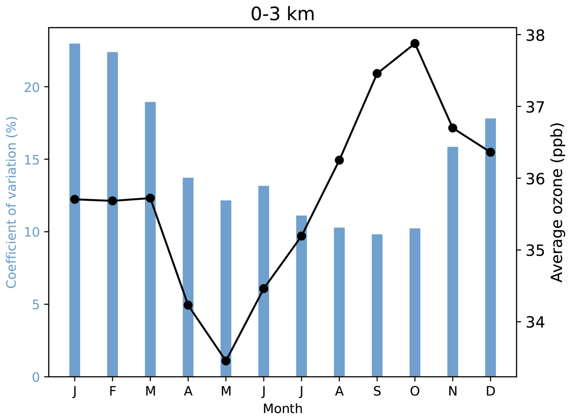
Figure 1 Evaluation of regional coefficient of variation (CV) and average of monthly mean ozone in the lowermost troposphere in 2017 over the Tropical Atlantic (25° S–25° N, 34–18° W). Light blue bar and black line indicate the coefficient of variation (CV) and average calculated from three products (IASI + GOME2, TCR-2 and CAMS reanalysis), respectively.

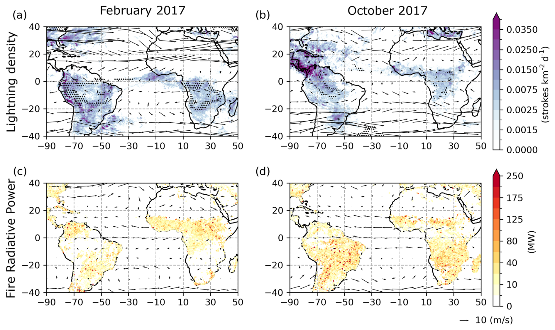
Figure 2 Monthly WGLC lightning density and fire radiative power (FRP) of presumed vegetation fire in (a, c) February and (b, d) October 2017. Winds at 3 and 10 km of altitude from ERA5 are indicated by black arrows in February and October, respectively. Black dots (a–b) indicate areas with OLR <220 W m⁻².

A previous intercomparison of four chemistry reanalyses including TCR-2 and CAMS reanalysis, suggests the largest SD at 850 and 650 hPa over South America, Central Africa, and Northern Australia (Huijnen et al. 2020). This is mainly associated with the differences of the representation of biomass burning emissions and its impact on ozone production among the systems. Estimates of CO emissions for African fires have been subject to considerable uncertainty because of the high variability of African fires in time and space (Andela and van der Werf, 2014). Two chemistry reanalysis products used in this study adopt different biomass burning emission inventories (Table 1). GFED used by TCR-2 is produced by using the bottom-up approach which uses burned area and fuel loads (van der Werf et al., 2017). GFAS (used by CAMS reanalysis) is produced by using the top-down approach which uses FRP data (Kaiser et al., 2012). Mismatches between bottom-up and top-down approaches have been discussed in previous studies (e.g., Stroppiana et al., 2010; van der Werf et al., 2006; Zheng et al., 2018). Evaluations of uncertainties of fire emissions and their impact on the ozone production are beyond the scope of this study.

Figure 3 shows horizontal distributions of monthly mean ozone and the CV in the lowermost troposphere in February and October 2017 in Fig. 1 as that with the second largest (February) and the second smallest (October) differences. In February 2017, the IASI + GOME2, TCR-2 and CAMS reanalysis products show high concentrations of ozone from Western Africa to the Gulf of Guinea (on the left panels of Fig. 3). An enhancement of ozone in the north of the St. Helena anticyclone between 10 and 20° S and centred at 20° W can be only observed by IASI + GOME2, whereas two chemistry reanalysis products show low ozone values below 20 ppb. Large CV seen over Brazil and Southern Africia corresponding to the regions which CAMS reanalysis shows low ozone concentrations. On the contrary, CV is small in the active fire region over Western Africa. It means that differences of ozone concentration among the datasets are small relative to their concentration. In the outflow from Western Africa over the Tropical Atlantic, large CV can be seen, which may be associated with differences of the representation of transport and convection. The second largest CV shown in Fig. 1 is attributed to and moderate CV over the North Atlantic between 10 and 40° N and large CV in the north of the St. Helena anticyclone. TCR-2 and CAMS reanalysis show relatively higher concentration of ozone over the Atlantic in the Northern Hemisphere as compared to IASI + GOME2.

In October 2017, the three products show high concentrations of ozone over the Tropical Atlantic in the Southern Hemisphere between Brazil and the Congo Basin (on the right panels of Fig. 3). High ozone concentrations are also observed over Western Africa, whereas relatively low concentrations are found near the equator. Large CV regions over the Amazon Rainforest and Central Africa are corresponding to the regions which CAMS reanalysis shows low ozone concentrations as in the case of February. While relatively large CV can be seen over the Equatorial Atlantic, CV over the Atlantic is smaller than that in February.

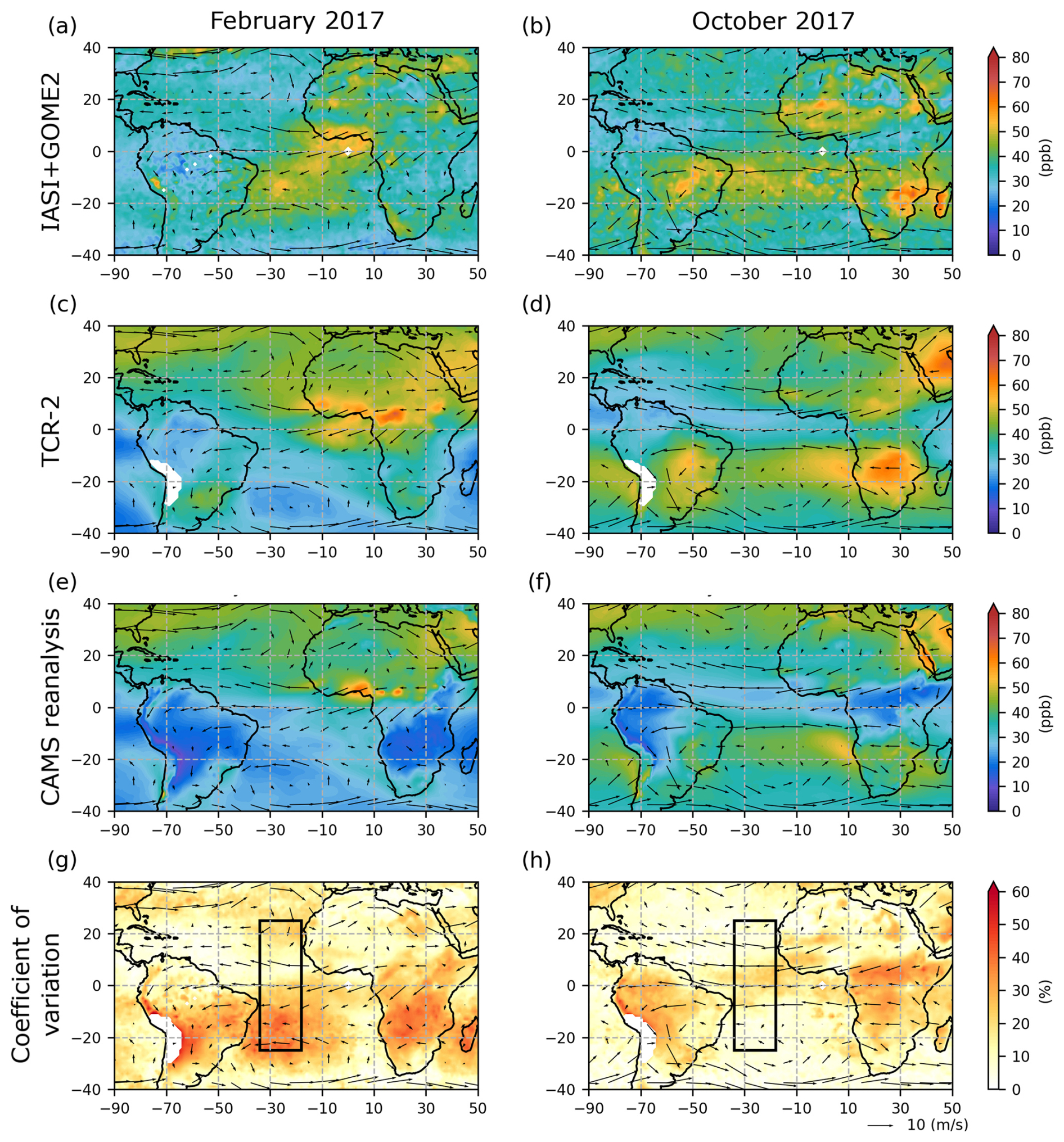
Figure 3 Distribution of monthly mean ozone from the surface to 3 km altitude in February and October 2017. (a, e) IASI + GOME2, (b, f) TCR-2, (c, g) CAMS reanalysis and (d, h) coefficient of variation. Winds at 3 km altitude from ERA5 are indicated by black arrows. Black rectangle (25° S–25° N, 34–18° W) indicates the region for which the average ozone and coefficient of variation that are shown in Fig. 1.

A rather different situation is seen for the ozone distribution depicted in the middle to upper troposphere. This is shown by Fig. 4 in terms of monthly mean ozone and the CV in the atmospheric layer between 6 and 12 km above sea level, in February and October 2017. All products show a horseshoe-shaped structure of high concentration ozone from Southern Africa to the east of Brazil (20° S) and until the Gulf of Guinea in February 2017 (on the left panels of Fig. 4). In October, high concentrations of ozone can be seen in the Congo Basin, Southern Brazil and the outflow over the South Atlantic. Moderate enhancement of ozone can be seen over the African Sahel. In this upper layer of the troposphere, more similarity can be observed between TCR-2 and CAMS reanalysis (Fig. 4). It might come from the influence of the assimilation of ozone satellite products.

The previous intercomparison of four chemistry reanalyses by Huijnen et al. (2020) suggests the large SD at 350 hPa over South America, Central Africa, and over the Arctic and Antarctic regions could reflect different representations of deep convection along with biomass burning emissions at low latitudes and polar vortex, stratospheric ozone intrusions and chemistry treatment at high latitudes among the systems. In the atmospheric layer between 6 and 9 km above sea level, CVs in February and October are generally larger than those in the lowermost troposphere because of lower ozone concentration of IASI + GOME2 as compared to the two reanalysis products (Fig. 4). In February, large CV regions over Southern Africa, the Amazon Rainforest and the Atlantic in the Northern Hemisphere are corresponding to the regions where IASI + GOME2 ozone concentration is low (Fig. 4a). In October, large CV regions can be seen near the equator and over the Atlantic in the Northern Hemisphere. This distribution of CV is also affected by lower IASI + GOME2 ozone concentration (Fig. 4b). The next sections discuss in detail these differences and compare them with in situ reference measurements performed by an aircraft during 13–15 February and 17–20 October 2017.

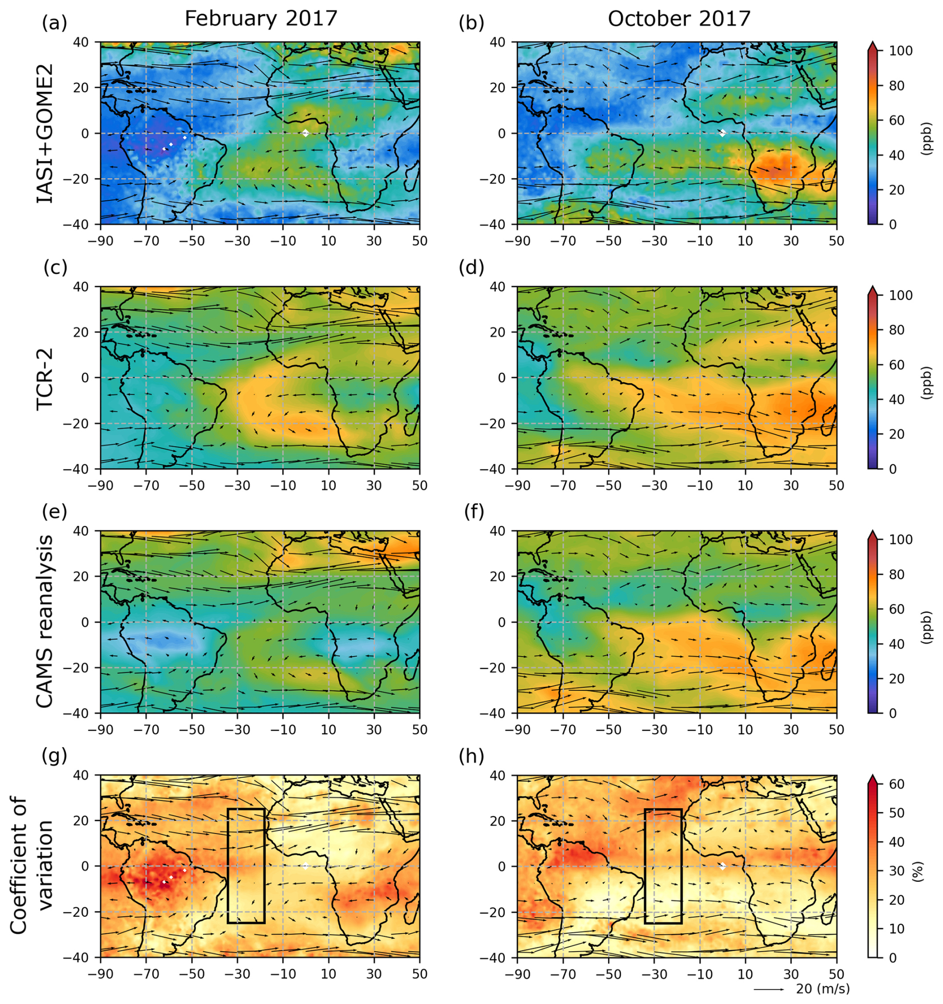
Figure 4 Distribution of monthly mean ozone from 6 to 9 km altitude in February and October 2017. (a, e) IASI + GOME2, (b, f) TCR-2, (c, g) CAMS reanalysis, and (d, h) coefficient of variation. Winds at 9 km altitude from ERA5 are indicated by black arrows. Black rectangle (25° S–25° N, 34–18° W) indicates the region for which the average ozone and coefficient of variation that are shown in Fig. 1.

3.2 Spatial distributions of tropospheric ozone during ATom campaign

In order to better understand the differences between atmospheric chemistry reanalyses and satellite observations, we use the observational data of the ATom airborne campaigns. We focus here on the periods and locations of ATom-2 and ATom-3 in situ observations of tropospheric ozone and CO in February and October 2017. The NASA DC-8 aircraft transect over the Atlantic on 13 and 15 February 2017 covers from south to north, respectively, from 53 to 8° S and from 8° S to 39° N (on each of these days, see the flight track on the left panels of Figs. 5 and 6). On 17, 19 and 20 October 2017, the transect covers the region from 53 to 7° S, from 7° S to 16° N and from 9 to 39° N (see the flight track on the right panels of Figs. 5 and 6). Therefore, we consider here concentrations of the three products (IASI + GOME2, TCR-2 and CAMS reanalysis) averaged for the periods from 13 to 15 February and from 17 to 20 October 2017.

Figures. 5 and 6 show the horizontal distributions of ozone for the period from 13 to 15 February and from 17 to 20 October 2017. These ozone distributions are generally similar to the monthly mean distributions of Figs. 3 and 4. During the period of ATom-2 from 13 to 15 February, all products show enhancements of ozone concentrations over active biomass burning areas near the coast of the Gulf of Guinea and over the nearby sea following the wind flow in the lowermost troposphere (10° S–10° N, panels on the left of Fig. 5). Only IASI + GOME2 shows high ozone concentration (>50 ppb) in the north of the St. Helena anticyclone (30–10° S over the ocean, Fig. 5a). TCR-2 and CAMS reanalysis show relatively higher concentrations in the Northern Hemisphere (>10° N) as compared to IASI + GOME2. In the middle troposphere, all products show the ozone plume forming a horseshoe-shape from Southern Africa to the east of Brazil (20° S) and until the Gulf of Guinea (panels on the left of Fig. 6). Especially, ozone concentrations from TCR-2 are the highest ones over the South Atlantic (about 80 ppb). IASI + GOME2 shows overall lower concentrations in comparison with the two reanalyses (Fig. 6a).

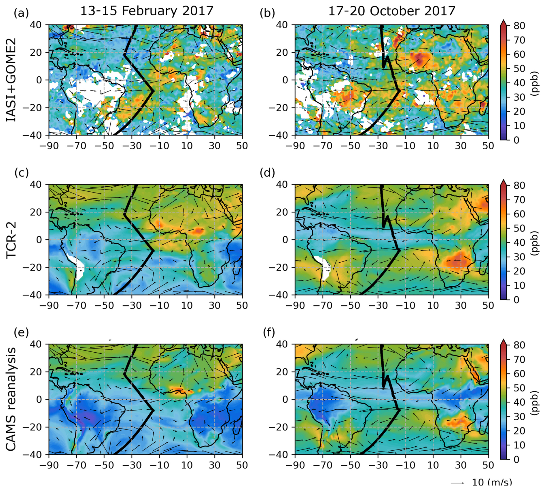
Figure 5 Distribution of mean ozone from the surface to 3 km altitude during 13–15 February and 17–20 October 2017. Black bold lines indicate the ATom-2 and ATom-3 flight tracks in (a–b) IASI + GOME2, (c–d) TCR-2 and (e–f) CAMS reanalysis. Winds at 3 km altitude from ERA5 are indicated by black arrows.

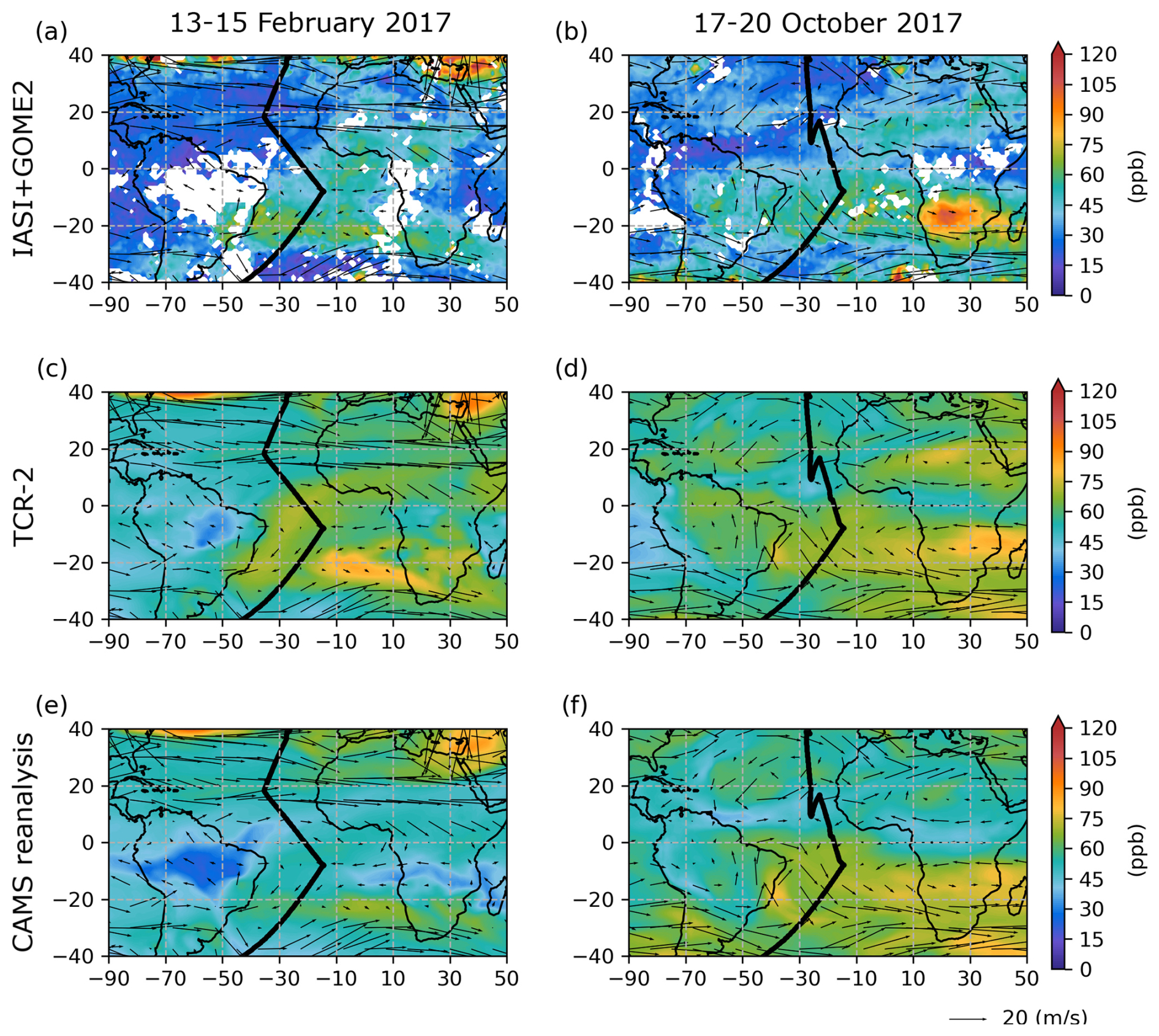
Figure 6 Distribution of mean ozone from 6 to 9 km altitude during 13–15 February and 17–20 October 2017. Black bold lines indicate the ATom-2 and ATom-3 flight tracks in (a–b) IASI + GOME2, (c–d) TCR-2 and (e–f) CAMS reanalysis. Winds at 9 km altitude from ERA5 are indicated by black arrows.

During the period of ATom-3 from 17 to 20 October 2017, all products show enhancement of ozone concentrations over the active biomass burning areas in Southern Africa and Brazil in the lowermost troposphere. Only IASI + GOME2 shows high ozone concentration (>60 ppb) over Western Africa (Fig. 5b). In the middle troposphere, all products show high concentrations of ozone in the Congo Basin, Southern Brazil and the outflow over the South Atlantic. Moderate enhancement of ozone can be seen over the African Sahel. IASI + GOME2 shows lower concentration as compared with the two reanalyses. The overall similarities between the ozone concentrations during 13–15 February and 17–20 October 2017 and the average over the whole month indicate that the aspects studied in the 3 and 4 d periods, such as the origins of tropospheric ozone (Sect. 3.3), are likely stable features representative of a larger period (at least a month).

3.3 Origins of ozone and CO reaching the Atlantic

To assess the difference among the products, we investigate the origins of ozone and CO by the ATom observations. Figures 7a and 8a show a classification of multiple air masses (stratospheric air, marine air, urban air, biomass burning air, mixed pollution air, and well-mixed and aged air) during ATom-2 and ATom-3 based on the method of Bourgeois et al. (2021). Here, well-mixed and aged air is defined as air mass with simultaneous low levels of biomass burning (HCN) and urban (C₂Cl₄) tracers. The other significant sources of CO (e.g., biogenic emissions and methane oxidation) and ozone precursors (e.g., lightning and soil emissions for NO_x, biogenic emission of VOCs) are included in the well-mixed and aged air mass category. This classification provides a very interesting picture of the complexity of the multiple contributions of the air masses along the transect.

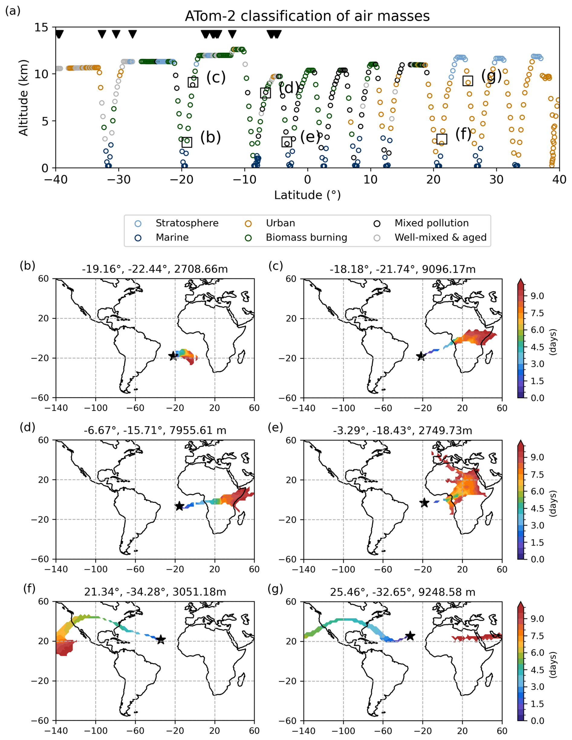
Figure 7 Classification and origin of air masses along the transect sampled by ATom-2. (a) Air masses are classified into six categories: marine (navy), stratosphere (light blue), urban (light brown), biomass burning (dark green), mixed pollution (black), and well-mixed and aged air (grey). Black inverted triangles indicate the well mixed and aged air influenced by lightning emissions. (b–g) Colours indicate average time since trajectories are initialized with NCEP winds.

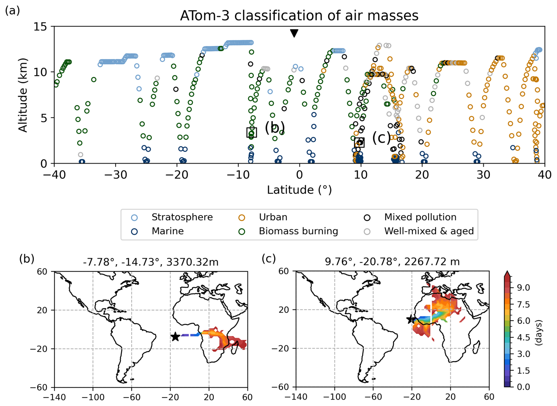
Figure 8 Classification and origin of air masses along the transect sampled by ATom-3. (a) Air masses are classified into six categories: marine (navy), stratosphere (light blue), urban (light brown), biomass burning (dark green), mixed pollution (black), and well-mixed and aged air (grey). Black inverted triangle indicates the well mixed and aged air influenced by lightning emissions. (b–c) Colours indicate average time since trajectories are initialized with NCEP winds.

To further analyse the chemical composition and origin of the air masses sampled along the transects, we illustrate the correlative variation of NO_x and HCN (the biomass burning tracer) concentrations measured by the aircraft during ATom-2 (Fig. 9a). Marine, urban, and mixed pollution air masses generally show low NO_x concentrations. Stratosphere, biomass burning, and well-mixed and aged air masses show higher NO_x concentrations. There are two possible sources of NO_x in well-mixed and aged air: boundary layer (including biogenic and soil emissions) and upper troposphere (lightning emission). To distinguish these two sources, we use probability of boundary layer influences (percentage of time the air masses are located within the boundary layer) determined by 30 d back trajectories provided by the ORNL DAAC (Ray, 2021; Fig. 9b). We define air masses influenced by lightning as those with high NO_x concentration (larger than the regional median of 0.033 ppb for ATom-2 and 0.054 ppb for ATom-3) and low probability of boundary layer influences (lower than 50 %). The significant influence of lightning is indicated by black triangles in Fig. 7a. Well-mixed and aged air masses with relatively high NO_x concentration in Fig. 9a show low probability of boundary layer influence or origin. Therefore, these air masses might be influenced by lightning emissions. The influence of lightning can be seen in the Southern Hemisphere during ATom-2 (Fig. 7a), whereas the influence is limited near the equator during ATom-3 (Fig. 8a).

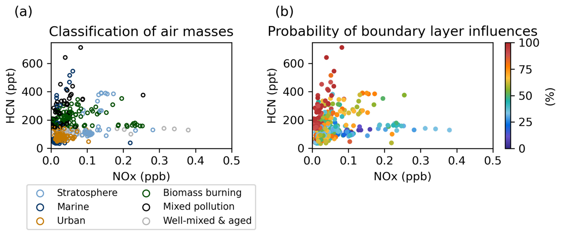
Figure 9 Scatter plots of NO_x vs. HCN (biomass burning tracer) of ATom-2 observation with colours indicating (a) the air masses classification into six categories: marine (navy), stratosphere (light blue), urban (light brown), biomass burning (dark green), mixed pollution (black), well-mixed and aged air (grey), and (b) the probability of boundary layer influences.

The capability to identify the origin and nature of air masses by IASI + GOME2 and IASI observations is illustrated in Fig. 10a is terms of the relationship of the abundance of CO and ozone, coloured according to their origin (derived from ATom-2 measurements). The concentrations derived from the two satellite products (IASI + GOME2 and IASI) and the two reanalysis products (TCR-2 and CAMS reanalysis) are extracted from the grid of the 1° × 1° datasets along the flight tracks of ATom-2. We remark a rather similar distribution of values as obtained for the scatter of values of HCN vs. NO_x in Fig. 9a. Urban-influenced air masses (light brown circles in Fig. 7a) are mostly associated with moderate abundances of both CO and ozone (up to respectively 150 and 60 ppb). Larger concentrations of ozone (>70 ppb) retrieved by IASI + GOME2 correspond to stratospheric air masses around 40° N. Some of these samples identified as influenced by the stratosphere and some as urban (as the air masses below, maybe due to a coarser vertical resolution of the satellite retrieval). CO-rich air masses correspond to those influenced by biomass burning, mixed-pollution and marine (with CO mixing down near the ocean surface). Whereas these features are clearly depicted by IASI + GOME2 and IASI observations, they are not clearly modelled by TCR-2 (Fig. 10c) and CAMS reanalysis (Fig. S4). The patterns distinguishing the chemical composition air masses are less clear.

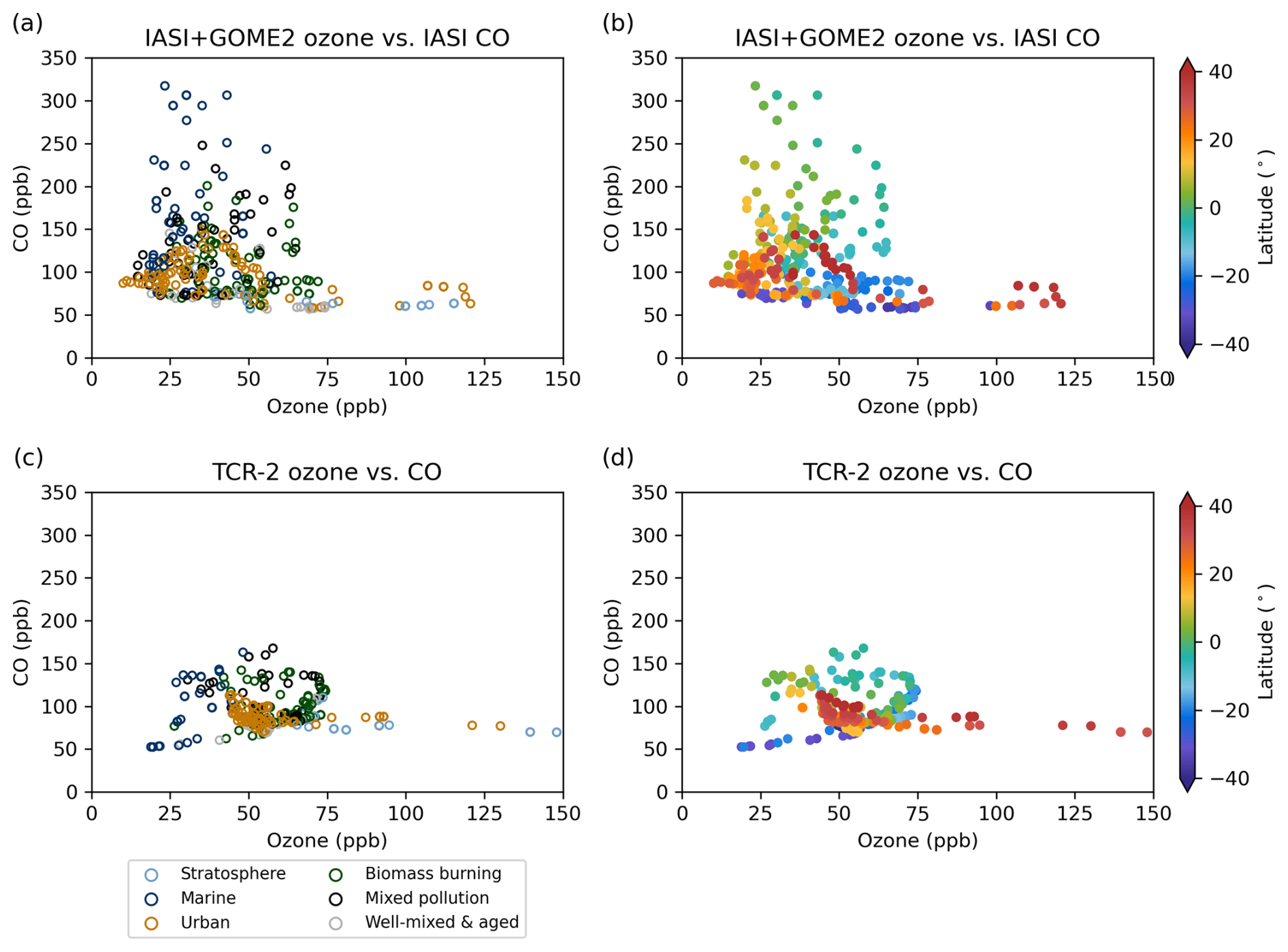
Figure 10 Scatter plots of CO vs. ozone for air masses sampled by ATom-2 derived from (a, b) satellite measurements of IASI and IASI + GOME2 and (c, d) TCR-2, respectively. Colours indicate (a, c) the air masses classification into six categories and (b, d) the latitude location.

3.4 Vertical distributions of tropospheric ozone and CO

This subsection provides a detailed analysis during ATom-2 and ATom-3, in terms of tropospheric ozone and CO distributions. The concentrations of three products (IASI + GOME2 and two reanalyses) are extracted from the grid of the 1° × 1° datasets along the flight tracks of ATom-2 and ATom-3 (Fig. 11). Tropospheric ozone is a secondary pollutant, which is both chemically produced and destroyed during transport in the atmosphere. Therefore, understanding its origin is a complex task. A first analysis of the origin of air masses rich in tropospheric ozone is presented here by investigating the vertical profiles of CO concentrations corresponding to satellite retrievals of CO derived from IASI measurements and CO concentrations derived from the two reanalyses (Fig. 12) in a similar way as done for ozone. We use the estimates of ozone and CO origins reaching the Atlantic (Sect. 3.3), and then, we intercompare the vertical profiles of three products (IASI + GOME2 and two reanalyses) to assess the accuracy of the satellite and reanalysis ozone products.

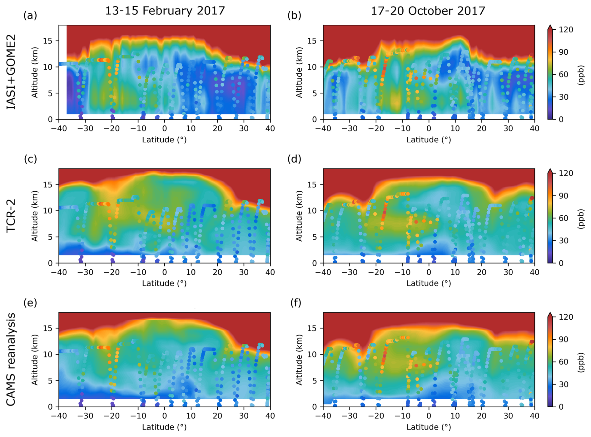
Figure 11 The ozone concentrations of (a–b) IASI + GOME2, (c–d) TCR-2 and (e–f) CAMS reanalysis are averaged for the period from 13 to 15 February 2017 and from 17 to 20 October 2017, respectively, and are extracted along the ATom flight tracks. Dots show vertical profiles of ozone concentrations from ATom-2 and ATom-3 observations for the periods from 13 to 15 February and from 17 to 20 October 2017.

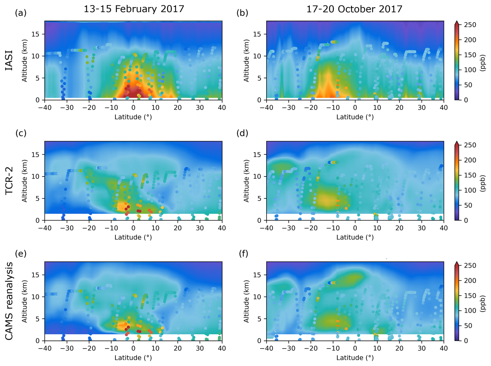
Figure 12 The CO concentrations of (a–b) IASI, (c–d) TCR-2 and (e–f) CAMS reanalysis are averaged for the period from 13 to 15 February 2017 and from 17 to 20 October 2017, respectively, and are extracted along the ATom flight tracks. Dots show vertical profiles of CO concentrations from ATom-2 and ATom-3 observations for the period from 13 to 15 February and from 17 to 20 October 2017.

3.4.1 The Southern Atlantic

At around 20° S in the upper troposphere, one satellite and two reanalysis ozone products and ATom-2 in situ observations clearly depict a stratospheric intrusion (the left panels of Fig. 11). Very low potential vorticity ($<-\mathrm{2}$ PVU) and downward motion from ERA5 also indicate downward transport of air masses from the upper troposphere and the lower stratosphere at around 20° S (Fig. S5a and c). The ozone plume extends from the upper troposphere at 20° S to the middle troposphere at the equator according to the reanalyses. Concomitant relative humidity with respect to the ozone plume is low (Fig. S5e), which is typical for stratospheric air. However, this ozone plume is also collocated with a moderate CO plume (the left panels of Fig. 12), which is not expected for pure stratospheric air. According to the classification shown in Fig. 7a, most of air masses within this plume correspond to stratospheric air, biomass burning air, well-mixed and aged air, or mixed pollution air. Back trajectory analysis indicates that the air is from Central and Eastern Africa (Fig. 7c–d). These results suggest that the ozone plume is influenced by both stratospheric exchanges and biomass burning emissions. Some well-mixed and aged air masses show high NO_x concentration and low probability of boundary layer influence (Fig. 7a). According to the discussion in Fig. 9, these conditions suggest the influence of lightning-produced NO_x as ozone precursor. Back trajectories confirm that these lightning-influenced air masses originate from a lightning active region in South America (Fig. 2a).

The ozone distribution of three products is characterized by an ozone plume in the troposphere between 30° S and 5° N below 10 km of altitude during ATom-2 (the left panels of Fig. 11). IASI + GOME2 depicts the ozone plume at 3–6 km, which is lower than the altitude of the plume shown by TCR-2 and CAMS reanalysis. This enhancement of ozone concentration in IASI + GOME2 corresponds to the one seen in the lower troposphere horizontal distribution over the South and Tropical Atlantic (Fig. 5a). The horizontal distributions of ozone from the two reanalyses present lower concentrations in the lowermost troposphere between 30° S and 5° N (Fig. 5c and e), as the ozone plume is located at higher altitude (>5 km) in this case (Fig. 11c and e).

The transect of ATom-2 in situ measurements and IASI + GOME2 shows a remarkable agreement, across the whole south-north track and within the whole troposphere (Fig. 11a). This agreement is clearly better than with respect to the two reanalyses. Both ATom-2 and IASI + GOME2 depict a similar structure of the ozone plume in the troposphere (2 to 7 km of altitude) located between 30° S to 5° N. At about 3 km, ATom-2 ozone concentrations are 68 ppb (20.1° S) and 54 ppb (19.1° S), near the values depicted by IASI + GOME2 (59–70 ppb between 19 to 21° S). Lower concentrations are shown by TCR-2 and CAMS reanalysis, respectively of 44–51 and 34–40 ppb. The region between 30° S to 5° N is where only IASI + GOME2 shows high concentration in the north of the St. Helena anticyclone (Figs. 3a and 5a). Chemical tracers suggest that most of the air masses are classified into marine air and biomass burning air at around 20° S (Fig. 7a) being stagnant over the South Atlantic (Fig. 7b). It suggests that the two reanalysis products underestimate the ozone concentration in the lower troposphere at around 20° S. In the middle troposphere (4–7 km), ATom-2 measure similar ozone levels as both IASI + GOME2 and TCR-2. On the other hand, ATom-2 shows larger concentrations in the upper troposphere at 11 km of altitude (>90 ppb) than the satellite and the two reanalysis products.

At around 25° S in the upper troposphere, the satellite and the two reanalysis ozone products clearly depict a stratospheric intrusion during the ATom-3 period (the right panels of Fig. 11). ERA5 data suggests downward transport by very low potential vorticity (<–2 PVU) and downward motion (Fig. S6a and c) at around 25° S. The ozone plume extends from the upper troposphere at 25° S to the middle troposphere at the equator according to the reanalyses. Concomitant relative humidity with respect to the ozone plume is low (Fig. S6e). This ozone plume shows low CO concentration (the right panels of Fig. 12), which is expected for pure stratospheric air. IASI does not seem to reproduce the shape of the CO plume. The feature of the stratospheric intrusion in ATom-3 is not clearly identifiable. According to the classification shown in Fig. 8a, most of air masses within this plume correspond to biomass burning air or mixed pollution air. This inconsistency may be attributable to the fact that satellite and reanalysis products represent several-day averages. When the aircraft passed over this region, it is probable that no stratospheric intrusion occurred.

The transect of ATom-3 in situ measurements and the two reanalysis products shows a remarkable agreement, across the whole south-north track and within the whole troposphere (the right panels of Fig. 12). This agreement is clearly better than with respect to IASI + GOME2. It means that the two reanalysis products during the ATom-3 period reproduce the distribution of ozone better than those during the ATom-2 period.

3.4.2 The Tropical Atlantic

For the period from 13 to 15 February, three products are characterized by a maximum of CO abundance around the equator in the lowermost troposphere (the left panels of Fig. 12). This is consistent with ATom-2 measurements of CO. Chemical tracers suggest that most of the air masses rich in CO near the equator and in the Southern Hemisphere are classified into marine air, biomass burning air or mixed pollution air (Fig. 7a). Back trajectory analyses indicate that these CO-enriched air masses in the lower and middle troposphere (15° S–15° N) passed over the Gulf of Guinea, Western, Central and Northern Africa (Fig. 7d–e). In February, biomass burning is active in Western (south of the Sahara) and Central Africa (Fig. 2c). These results indicate that the biomass burning emissions with rich-CO are transported from the southern part of Western Africa and Central Africa to the remote Tropical Atlantic via the Gulf of Guinea by southeasterly winds. On the other hand, ozone concentration in the lower troposphere around the equator is moderate according to the three products and ATom-2 observations (the left panels of Fig. 11). This is consistent with significant sinks of ozone often encountered within a lower tropical marine troposphere. In these conditions, the photochemical lifetime of ozone is typically reduced to a few days because of abundant actinic radiation, ample water vapor, and negligible NO_x (e.g., Crutzen et al., 1999). The high abundance of water vapor in the equatorial region is confirmed by ERA5 reanalyses (Fig. S5e).

Strong upward motion can be observed around the equator (Fig. S5c). High relative humidity can also be observed in the middle and upper troposphere as well as in the lower troposphere around the equator (Fig. S5e). These results indicate that the air in the marine boundary layer is uplifted to the upper troposphere by the deep convection, as indicated by collocated OLR below 220 W m⁻² (Fig. 2a).

The CO concentrations retrieved by IASI are in good agreement with those measured by ATom-2 (>250 ppb), which are clearly higher than the CO abundance in the reanalysis products. At about 5° S, the CO peak located at 2–3 km of altitude is underestimated by two reanalyses as compared to the ATom-2 observations. This CO maximum is composed of three CO plumes: from surface to the middle troposphere (15° S–15° N), from the middle troposphere to the upper troposphere (25° S–5° N) and in the upper troposphere (10° S–20° N). ATom-2 measurements are consistent with these CO enhancements in the upper and middle troposphere.

For the period 17 to 20 October, three products are characterized by a maximum of CO abundance between 20° S and the equator in the lower troposphere (the right panels of Fig. 12). At about 20–10° S, the CO maximum underestimated by the two reanalyses is located at 2–7 km of altitude. ATom-3 observation indicates an enhancement of CO in the upper troposphere at about 10° S. Only CAMS reanalysis reproduces this enhancement (Fig. 12f).

The CV in October is smaller than that in February as shown in Sect. 3.1 (Fig. 1). In the lowermost troposphere, a moderate CV can be seen near the equator because IASI + GOME2 ozone is higher than the others (the right panels of Fig. 3). The transect of ATom-3 in situ measurements and the two reanalysis products shows a remarkable agreement (the right panels of Fig. 11). In the lowermost troposphere around 20° S–20° N, back trajectories indicate that the air masses originate from the African continent (Fig. 8b–c). Most of the air mass is classified to marine air and biomass burning air (Fig. 8a).

3.4.3 The Northern Atlantic

The two reanalyses show a stratospheric intrusion in the UTLS around 25° N, co-located with a descending branch of the Hadley cell (Fig. S5c), whereas IASI + GOME2 does not show such a feature during ATom-2 (the left panels of Fig. 11). In this region, we remark high potential vorticity, low relative humidity (Fig. S5a and e) and strong subsidence at altitudes between 6 and 10 km (Fig. S5c). The downward motion speed derived from ERA5 reanalyses is greater than 1 cm s⁻¹ in absolute terms, which is significantly larger than the typical value for tropical clear-sky regions (Gettelman et al., 2004; Das et al., 2016). The CO concentrations collocated with the ozone plume are low (the left panels of Fig. 12).

During ATom-2, we clearly depict a strong urban influence north of 10° N between 2 and 10 km of altitude, a sector with rather weak ozone abundance according to satellite and in situ measurements (Figs. 7a and 11a). Biomass burning emissions notably affect the lower-to-upper troposphere (from 2 to 11 km of altitude) roughly between 25° S to 5° N, which are collocated with moderate and large abundances respectively ozone and CO (Fig. 12a) much likely associated with emissions from Central African fires (Fig. 2c).

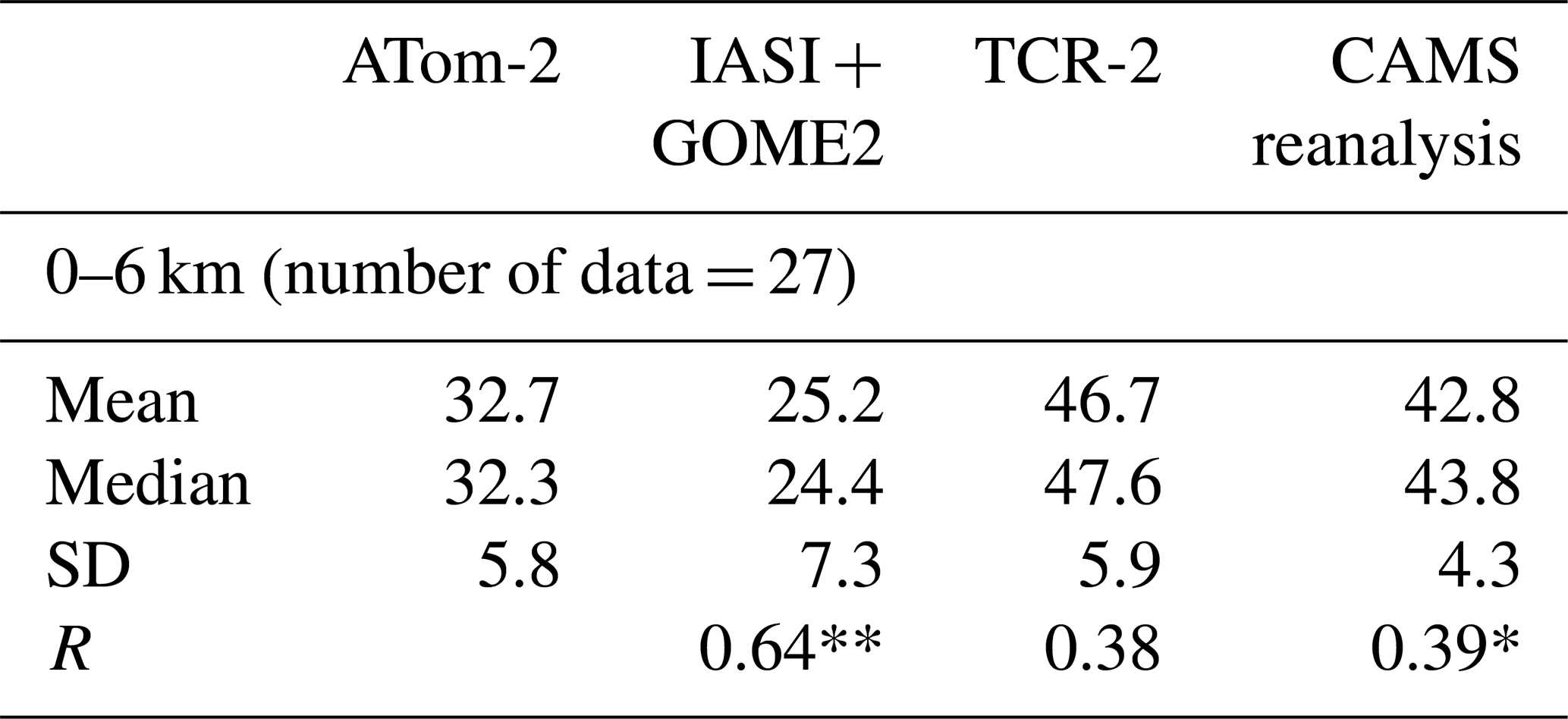
In the Northern Hemisphere (north of 5° N and until 35° N), a clear decrease of ozone concentrations within the troposphere (down to about 30 ppb) is clearly observed by both ATom-2 and IASI + GOME2 (Fig. 11a). On other hand, none of two reanalyses depict such ozone reduction (Fig. 11c and e). A quantitative assessment of the difference in the Northern Hemisphere to evaluate their capability is presented in Table 2. We compare ozone concentrations of three products (IASI + GOME2 and two reanalyses) with ATom-2 between 10 and 30° N. In the lowermost troposphere, IASI + GOME2 shows lower mean concentration (25.2 ppb) compared to ATom-2 (32.7 ppb), whereas the other reanalysis products show much higher concentrations. Mean ozone concentrations from TCR-2 and CAMS reanalysis are 10–14 ppb higher. We find a robust correlation between IASI + GOME2 and ATom-2 ozone concentrations (R=0.64, p value <0.05). These results suggest that the ozone concentration over the Atlantic in the Northern Hemisphere is overestimated by two chemistry reanalyses in the lower troposphere, while the best agreement with ATom-2 is clearly seen for IASI + GOME2 in correlation and absolute values.

Table 2 Summary ozone statistics for the lower troposphere (0–6 km) along the ATom-2 flight track between 10 and 30° N. R is correlation coefficient with respect to ATom-2. Asterisk denotes statistical significance at p value <0.05 (*) and p<0.01 (**).

A moderate CV is observed in the Northern Hemisphere in February because TCR-2 and CAMS reanalysis show relatively higher concentration of ozone over the Atlantic as compared to IASI + GOME2 (the left panels of Fig. 3). Below the UTLS around 20–25° N, back trajectories from the lower and upper troposphere indicate that the air masses originate from North America (Fig. 7f–g). Most of the air mass is classified to urban air in the Northern Hemisphere, especially over 20° N (Fig. 7a). The influence of biomass burning is seen closer to the equator. These results suggest that the reanalyses likely overestimate the urban influence of the Northern Hemisphere over the Atlantic.

During ATom-3, strong urban influence can be also seen north of 20° N between 2 and 10 km of altitude (Fig. 8a). Biomass burning emissions notably affect the lower-to-upper troposphere (from 2 to 11 km of altitude) roughly between 40° S to 10° N much likely associated with emissions from Central and Southern African fires (Fig. 2d).

ATom-3 and two reanalysis products show similar ozone concentrations in the Northern Hemisphere. IASI + GOME2 depicts the ozone plume at 3–6 km, which is lower than the altitude of the plume shown by the reanalysis products. A moderate enhancement of ozone can be seen north of 10° N. These enhancements of ozone concentration correspond to those seen in the lower troposphere horizontal distribution over the Atlantic (the right panels of Fig. 5). The horizontal distribution of ozone from the reanalyses presents lower concentrations in the lowermost troposphere around the equator (Fig. 5d and f). Particularly in the Northern Hemisphere (north of 10° N), we can observe large difference of ozone concentration between IASI + GOME2 and two reanalyses (the right panels of Fig. 11). This difference corresponds to concentrations 20 ppb lower for IASI + GOME2 than for the reanalyses. In addition, an enhancement of ozone from the upper troposphere to the middle and lower troposphere can be observed in reanalyses around 25° N. However, IASI + GOME2 shows only an enhancement of ozone concentrations up to 40 ppb in the lower troposphere around 15° N.

The previous study of the ATom campaign by Bourgeois et al. (2021) concluded that three global chemical transport models systematically underpredicted the observed influence of biomass burning on tropospheric ozone. In the Northern Hemisphere fall and winter, biomass burning and urban emissions contribute similar levels of ozone. In the Tropical Atlantic and the Southern Hemisphere fall and winter, biomass burning emissions contribute ∼2 to 10 times more ozone than urban emissions. We analyse the two ATom campaign periods in February and October. Although both periods are included in fall and winter in the Northern Hemisphere, the features of CV are different. Our results suggest that the seasonal variability of biomass burning in African should be considered when evaluating model uncertainty of tropospheric ozone over the Atlantic.

4 Conclusions

We have presented an analysis of the tropospheric ozone spatial distribution and its origins using satellite (IASI + GOME2), in situ observations (ATom-2 during 13–15 February and ATom-3 during 17–20 October 2017) and two global reanalyses (TCR-2 and CAMS reanalysis) over the Tropical and South Atlantic. Seasonal variation of regional discrepancies (expressed as spatial coefficient of variations) between the satellite observations and the reanalyses of monthly ozone distribution over the Tropical Atlantic (25° S–25° N, 34–18° W) show a clear seasonality corresponding to two biomass burning seasons and two transition seasons in Africa. The largest CV among these datasets are seen for the months of January and February. In this last period, the region is likely influenced by biomass burning emissions from the southern part of West Africa and Central Africa and deep convection over the Gulf of Guinea (over the Ocean) and Central and Southern Africa (as depicted by the frequent lightning activity). On the contrary, the highest average ozone and small CV can be seen in October, corresponding to the biomass season in the Southern Hemisphere. Comparisons of horizontal distributions of monthly ozone in the lowermost troposphere (surface–3 km) in February 2017 show that IASI + GOME2, TCR-2 and CAMS reanalysis datasets display high concentration of ozone from Western Africa to the Gulf of Guinea. Only IASI + GOME2 depicts an enhancement of lowermost tropospheric ozone north of the St. Helena anticyclone. In the middle and upper troposphere, all products show a horseshoe-shaped structure of high concentration of ozone from Southern and Western Africa to the east of Brazil. IASI + GOME2 show lower ozone concentration in the South America compared to two chemistry reanalysis products. In October 2017, three products display high concentrations of ozone between Brazil and the Congo Basin and over Western Africa in the lowermost troposphere. In the middle and upper troposphere, more similarity can be observed between the reanalyses in owing to the influence of the assimilation of ozone satellite products. All products show high concentrations of ozone in the Congo Basin, Southern Brazil and the outflow over the South Atlantic. Moderate enhancement of ozone can be seen over the African Sahel.

The tropospheric ozone spatial distributions are generally similar for the monthly means in February and October 2017 and the average in the 3 and 4 d periods when ATom-2 and ATom-3 in situ measurements are available. We analyse these vertical profiles along a south-north track from 40° S to 40° N to assess the capability of satellite and chemistry reanalysis products to characterize the spatial distribution of the tropospheric ozone over the Tropical Atlantic. The origins and vertical distribution of tropospheric ozone are strongly shaped by a complex mixture of influences from African biomass burning, lightning, stratospheric intrusion and long-range transport of urban emissions. We clearly observe that only the IASI + GOME2 satellite approach is able to describe the strong gradient of significant tropospheric ozone enhancements in the Southern Hemisphere and low abundances in the Northern Hemisphere, in agreement with ATom-2 in situ measurements. An enhancement of ozone in the north of the St. Helena anticyclone between 10 and 20° S is consistently observed by both IASI + GOME2 and ATom-2, whereas the two reanalyses show low ozone values below 20 ppb. North of the equator, all two reanalyses particularly fail to depict the weak ozone concentrations consistently observed by satellite and in situ sensors (IASI + GOME2 and ATom-2 agree both in absolute values and correlation). This is partly explained by a significant ozone enhancement displayed by the two chemistry reanalyses in the descending branch of the Hadley cell at around 25° N, which is not depicted by IASI + GOME2 nor ATom-2. Air masses in the Northern Hemisphere with weak concentrations of ozone (over 20° N) are classified as influenced by urban sources (from North America according to back trajectories). These results suggest that the reanalyses overestimate the abundance of tropospheric ozone over the remote locations in the Tropical Atlantic for air masses influenced by urban sources of North America in February 2017. In the Southern Hemisphere, two reanalysis products underestimate the ozone concentration in the lower troposphere at around 20° S. Chemical tracers suggest that most of the air masses are classified into marine air and biomass burning air being stagnant over the South Atlantic. These results suggest that the reanalyses likely underestimate the biomass burning influence of the Southern Hemisphere in the lower troposphere.

On the other hand, the reanalysis products reproduce the distribution of ozone relatively well during the ATom-3 period. The previous study by Bourgeois et al. (2021) revealed that models systematically underpredict the observed influence of biomass burning on tropospheric ozone based on the estimates using classical four seasons. Our findings suggest intercomparison studies over the Atlantic should be carried out using seasons based on the location of active biomass burning areas as well as the influence of anthropogenic precursors over Northern Atlantic. Such studies will improve the accuracy of chemistry-transport models in this region.