Emitted yesterday, polluting today: temporal source apportionment of fine particulate matter pollution over Central Europe

Fine particulate matter (PM_2.5) pollution remains a critical health issue in Europe. While numerous studies have quantified the spatio-sectoral sources of urban PM, the temporal origin has received minimum attention. This study addresses this gap by developing a Temporal Source Apportionment approach within the CAMx chemical transport model to quantify the long-term contributions of emissions from the preceding 14 d to PM concentrations, focusing on the 2010–2019 period and Central Europe. The novelty of the study lies in a long term and continuous adoption of TSA unlike previous attempts to quantify the age distribution of polluting aerosol that focused on selected air pollution periods.

The results show that current-day emissions dominate winter PM_2.5, contributing 30 %–60 % on average, while day-1 emissions add further 20 %–30 %. Contributions decrease with emission age, falling below 5 % after 3 d and becoming negligible beyond 7 d. Secondary inorganic aerosols and primary organic aerosols exhibit similar patterns, although for winter nitrate levels, the highest contribution comes from day-1 emissions, reflecting the time needed for chemical formation. Summer contributions are smaller due to enhanced mixing and faster removal, whereas biogenic emissions also contribute largely, giving anthropogenic emissions a smaller role.

Importantly, while the average contribution of older emissions is low, occasional episodes show substantial impacts: day-4 emissions can contribute up to 10 %, and even week-old emissions can add 2 % in winter. These findings emphasize that adverse air quality episodes are influenced not only by same-day emissions but also by pollution accumulated from previous days resulting from past emissions. Effective mitigation policies on PM pollution must therefore consider reducing emissions several days in advance of predicted pollution episodes, rather than relying solely on same-day interventions.

1 Introduction

Despite overall improvements in urban particulate matter (PM) pollution in Europe, EU standards are still not met in many urban agglomerations. According to the European Environmental Agency's 2024 air quality status report (EEA, 2024) while considering WHO guidelines, 95 % of urban population is exposed to unhealthy concentrations of PM_2.5 (PM with diameter less than 2.5 µm), especially in central and southeastern Europe. Given the health effect of PM pollution, ranging from premature death in people with heart or lung disease, non-fatal heart attacks, aggravated asthma, decreased lung function, and increased respiratory symptoms (Kim et al., 2015), PM pollution represents a significant deteriorating factor of living conditions in urban areas. Therefore, there is a need to understand the sources (Crippa et al., 2019; Bartík et al., 2024), drivers (Yang et al., 2023; Huszar et al., 2024), and the overall characterization of the aerosol composition to be able to mitigate the health impacts of aerosols (El Haddad et al., 2024) in urban areas.

There are numerous causes of PM pollution in cities. They can be divided into two main categories: (i) those acting directly and the (ii) indirect causes. Probably the most important direct cause are local (urban) emissions (Thunis et al., 2021). Many studies have shown that local sources contribute by many tens of percent to annual PM levels in cities. E.g. Skyllakou et al. (2014) and Huszar et al. (2016) showed for Paris and other cities in Europe that the contribution of local sources can reach 50 %. However, this also means that regional (rural) emissions also contribute to urban PM concentrations. This was calculated even earlier by Im and Kanakidou (2012) who found about 30 % contribution of regional sources to PM levels in two Mediterranean megacities, Athens and Istanbul. Also, Panagi et al. (2020) showed using a tracer approach that around half of Beijing pollution is transported from other areas. More recently, Huszar et al. (2021) calculated very similar contributions from local sources to urban PM, which was confirmed by Huszar et al. (2024). In summary, there is a consensus that while local sources represent a significant cause of urban pollution, rural contributions to urban PM abundances can have a comparable magnitude. Moreover, transport of pollution from distant regions up to transcontinental transport can be another factor that worsens urban air pollution in European cities (e.g. Makra et al., 2011; Paschalidou et al., 2015; Bodor et al., 2020) and over other regions of the world (e.g. Mo et al., 2021; Velásquez-García et al., 2024). Lastly, urban PM pollution can also be deteriorated by natural emissions such as wind-blown dust (Liaskoni et al., 2023), wildfires (Mani et al., 2023) or sea spray aerosol emissions (SSA; Athanasopoulou et al., 2008). It has to be also emphasized, that many of these studies analyzed the short-term impact of emissions spanning at most a few months (i.e. focusing on a season), both local/regional and long-range to PM burdens while at the same time, there is a rather limited research on the long-term “climatological” impact that span multiple years or even decades. Previously, Huszar et al. (2016) searched for answer to what extent regional emissions impact urban air pollution levels giving some hint to long term contribution of rural emissions in urban PM levels. More recently, Huszar et al. (2021) analyzed the similar impact for multiple year. Panagi et al. (2020) also considered a 4 year period to debunk the regional contributions to Beijing air pollution. Mo et al. (2021) calculated the long range transport impact on surface fine PM in China for a 5 year period. Unlike studies focusing on seasons or only some short air pollution episodes, the listed studies give information about the long term behavior or pollution regimes and their causes. On the other hand, short term studies can point to extreme conditions that are hindered in long term perspective.

In addition to the role of emissions in reducing urban air-quality, a large role is attributable to meteorological conditions. During the cold months, situations with stagnant conditions that mean low winds and low heights of the planetary boundary layer (and reduced vertical mixing) support the building up of large abundances of particular matter (He et al., 2017; Miao et al., 2019) while also increased humidity can correlate with high PM pollution in urban centers, as shown by Zalakeviciute et al. (2018).

Indirectly, urban PM pollution can be amplified or at least modulated also by meteorological changes caused by the urban land-surface and urban canopy (Oke et al., 2017; Karlický et al., 2020; Villalba-Pradas et al., 2025; Karlický et al., 2026). For decades, it has been known that due to distinct geometric features (buildings, street canyons) covered with artificial materials (asfalt, concrete), urban temperatures are higher than in rural areas, which led to the introduction of the Urban Heat Island concept (UHI) (Oke, 1982). However, in addition to temperature, other meteorological variables are also modified in urban environments. Due to rainwater runoff and suppressed evaporation due to limited vegetation, specific humidity is also reduced (Chakraborty et al., 2022). Furthermore, because of the enhanced drag, the wind speeds are also reduced (Jacobson et al., 2015; Huszar et al., 2018a, b; Zha et al., 2019). At the same time, due to larger vertical wind gradients and thermal effects, the vertical eddy diffusion in cities is greatly enhanced (Ren et al., 2019; Huszar et al., 2020a; Wei et al., 2018; Wang et al., 2021) which leads, in general, to thicker boundary layer (Wang et al., 2021).

It is clear, that modified meteorological conditions due to the effects listed above must lead to modifications in pollutant concentrations as these influence transport, chemical formation and decay, deposition etc. The so called urban canopy meteorological forcing (UCMF), introduced by Huszar et al. (2020a) summarizes these effects in a common framework. Indeed, many have shown that UCMF leads to significant modifications in PM pollution in cities. While decreased winds result in build-up of PM around sources (e.g. Huszar et al., 2018b; Zhu et al., 2017; Li et al., 2019), increased vertical eddy transport leads to decreases of concentrations (Li et al., 2019; Huszar et al., 2020b) with the net effect being a decrease of PM pollution due to overall UCMF as shown by Huszar et al. (2020a). Moreover, it was also shown that over urban areas, dry deposition of PM is increased which leads further decrease of PM concentrations.

In summary, there have been numerous attempts to answer where the urban PM pollution originates and what are the drivers and modulators. The first question was answered by quantifying the contribution of different sources, while the second looked at the impact of meteorological conditions and other effects like deposition. However, none of these studies investigated in detail when were these PM or their precursors emitted. Is adverse urban pollution the results of the emissions on the same day or aged PM emitted during previous days can contribute too, and if so, to what extent? In general, can the contribution of emissions from previous days (or weeks) be significant?

These are relevant questions, as aerosols have lifetimes in the order of several days (up to 1–2 weeks), depending, of course, largely on the aerosol type (primary vs. secondary) (Hodzic et al., 2015; Geo et al., 2022) and the driving meteorological conditions (Kristiansen et al., 2016). This implies that aerosol emitted a few days earlier can potentially still contribute significantly (Sharma et al., 2016). This has of course relevance for policy emission controls, putting emphasis on limiting emissions before potentially adverse pollution episodes occur, as was shown by Ansari et al. (2021). This later study however examined only one particular agglomeration in China and for a selected high pollution episode without giving answer on long term contributions of emissions from previous days on the pollution on a chosen day. Similarly, Ying et al. (2021) made an attempt to characterize the age-distribution of both primary and secondary aerosol by tagging the emissions by the time of emission release, but analyzed only one winter month without assessing the long-term contribution of emissions at different times. There are other examples of calculating the age distribution of PM, Wagstrom and Pandis (2009) being one of the first such, but they also analyzed only a few days. Later, Zhang et al. (2019) developed a similar method, however applied it only to elemental carbon. Xie et al. (2023) have chosen a similar approach too, but they used hourly age bins for a 96 h period for one selected haze event, again not providing an answer to the above mentioned questions regarding the long term contribution of past emissions (even those older than 96 h, i.e. 4 d).

Our pioneering study aims to fill these gaps and tries to answer the above formulated questions using a chemical transport model based approach for a present day 10 year long period, focusing on the area of central Europe. The approach is based on tagging emission by the day when they have been emitted and quantifying the contributions of different days (the current and previous ones) on the concentrations for a given time.

2 Methodology

2.1 Models used

In this study, the chemistry transport model (CTM) calculations were performed using the Comprehensive Air Quality Model with Extensions (CAMx) version 7.20 offline driven by the Weather Research and Forecasting model couple (WRF) version 4.4 with time resolved emission inputs prepared using the Flexible Universal Processor for Modeling Emissions (FUME) emission preprocessor. The detailed description of these models follows, including their specific configuration.

WRF is a mesoscale non-hydrostatic meteorological model and in this study the version with online coupled chemistry (WRF-Chem) was adopted. However, only the meteorological outputs of WRF-Chem were used (the chemical model outputs from these simulations were used in the Prieto Perez et al., 2025 validation study). Detailed description of this model is provided by Grell et al. (2005), while for boundary layer physics, convection, cloud/rain microphysics and radiation the BouLac (Bougeault and Lacarrere, 1989), Grell 3D (Grell, 1993), Purdue Lin (Chen and Sun, 2002) and RRTMG (Iacono et al., 2008) schemes were activated, respectively. The atmosphere-surface exchange was parameterized using the Noah land-surface model (Chen and Dudhia, 2001) along with the Eta model for the description of the surface physics (Janjić, 1994) and Single-Layer Urban Canopy Model (SLUCM) to parameterize the urban canopy effects (Kusaka et al., 2001). The above mentioned combination of parameterization is based on a detailed validation of the WRF model for central Europe (Karlický et al., 2020) while this combination showed the best match with observations.

The model CAMx is a comprehensive state-of-the-art Eulerian chemistry transport model aimed at both detailed photochemistry and aerosol chemistry and is described in Ramboll (2022). It implements multiple gas-phase chemistry schemes (Carbon Bond 5 and 6, SAPRC07TC, etc.), while, in this work, the Carbon Bond 6 revision 5 (CB6r5) chemistry mechanism was invoked. To complete the atmospheric chemistry with aerosol physics, a static two-mode (CF; coarse-fine) approach was considered. To account for the secondary inorganic aerosol formation, the ISORROPIA thermodynamic equilibrium model (Nenes et al., 1998) was invoked. Secondary organic aerosol (SOA) was partitioned from its gas-phase precursors applying the SOAP equilibrium scheme (Strader et al., 1999). Some limitation of this scheme is that aging of organic aerosol is not considered. This can however impact on aerosol lifetime (Rudich et al., 2007), e.g. Georgopoulou et al. (2025) showed that aging of organic aerosol due to oxidation increase its water solubility which can enhance its wet removal resulting in lower life-times.

The Seinfeld and Pandis (1998) and Zhang et al. (2003) methods were used for wet and dry deposition, respectively. An important capability, used also in this study, is the Particulate Source Apportionment Technology (PSAT), which is a tool implemented in CAMx to track emission contributions to PM species concentrations. PSAT provides PM attribution for a given emission matrix but does not provide quantitative information as to how PM contributions would change as emissions are altered (i.e. sensitivity) due to the non-linearity of the chemistry. PSAT is designed to apportion the following classes of CAMx PM species: sulfur, nitrogen, SOA, primary PM and particulate mercury (HgP; not used in this study).

CAMx was driven offline by hourly WRF model output converted to CAMx-ready meteorological input files using the wrfcamx preprocessor, which is provided along with the CAMx code at https://www.camx.com/download/support-software (last access: 14 November 2025). Due to offline coupling, no feedback on radiation was considered. However, it is rather small above the area in focus (Huszar et al., 2012). Vertical eddy diffusion coefficients (Kv) are not provided in WRF output and had to be diagnosed from the available meteorological parameters (like wind, temperature, and humidity profiles) using the diagnostic approach implemented in the CMAQ model (Byun and Ching, 1999).

Finally, for processing the annual anthropogenic emission totals (see the next section) into hourly speciated emission fluxes interpolated to the model grid, we applied the “in-house” emission preprocessor called Flexible Universal Processor for Modeling Emissions (FUME; http://fume-ep.org/, last access: 15 July 2025; Belda et al., 2024).

2.2 Experimental setup and data used

Model simulations were conducted over a “larger” central European domain at 9 km × 9 km horizontal resolution with 189 × 165 grid boxes in the WE and NS direction, centered over the Czech capital, Prague (50.075° N, 14.44° E) using Lambert conic conformal projection. The domain thus spans approximately from France to Ukraine and from northern Italy to Denmark. In vertical, the WRF model uses 40 layers with the model top at 50 hPa (about 20 km a.s.l.) while the lowermost layer is approximately 30 m thick. CAMx is run on 18 vertical layers up to about 12 km. We simulated the 2010–2019 period and considered it as present-day conditions. The years affected by the COVID-19 pandemic 2020–2022, that faced strong emission reductions (Guevara et al., 2021), were therefore not included.

The WRF simulation was driven by the ERA5 reanalysis (Hersbach et al., 2023) while the CAMx was initialized and driven using the CAM-Chem global model simulation nudged towards the MERRA2 reanalysis as chemical boundary conditions (Buchholz et al., 2019; Emmons et al., 2020). We are aware of this inconsistency between the meteorology used to drive the WRF model (ERA5) and the meteorology used to nudge the global model serving the chemical boundary conditions (MERRA2), but we assume this to be negligible. Land-use fields for both the WRF model and for the dry-deposition in CAMx's Zhang model, are derived from CORINE Land Cover data, version CLC 2012 (CORINE, 2012).

2.2.1 Emissions

The European CAMS (Copernicus Atmosphere Monitoring Service) version CAMS-REG-APv1.1 inventory (Regional Atmospheric Pollutants; Granier et al., 2019) for 2015 was used as anthropogenic emissions data for the entire 10 year period. Figure S1 in the Supplement shows that this year is somewhat below the 2010–2018 average of the emissions (expect ammonia) so this could lead to some underestimation of the PM (as will be seen later in the Validation part). This was combined with high resolution Czech national emission data, the Register of Emissions and Air Pollution Sources (REZZO) dataset issued by the Czech Hydrometeorological Institute (http://www.chmi.cz, last access: 15 July 2025) and the ATEM Traffic Emissions dataset provided by ATEM (Ateliér ekologických modelů – Studio of ecological models; http://www.atem.cz, last access: 15 July 2025) while both emission inventories are from the same year as the CAMS emissions. As already mentioned, the FUME emission preprocessor was used to redistribute the emission data into the model grid. To speciate non-methane volatile organic compound (NMVOC) and PM emissions and obtain hourly emissions fluxes, speciation profiles and time-disaggregation factors from Passant (2002) and van der Gon et al. (2011) were used, respectively. Emissions of hydrocarbons for terrestrial ecosystems (mostly biogenic volatile organic compounds - BVOC) were calculated offline using MEGANv2.1 (Model of Emissions of Gases and Aerosols from Nature version 2.1) with the algorithm described by Guenther et al. (2012) driven by WRF meteorological fields (short-wave radiation, temperature, humidity, soil moisture, etc.). It has to be emphasized here that as emissions have no inter-annual variation during the analyzed period (2010–2019), the variability of the results including the extremes presented are driven by the variability of the meteorological conditions and partly also by the variability of the biogenic emissions which are coupled to varying meteorological conditions.

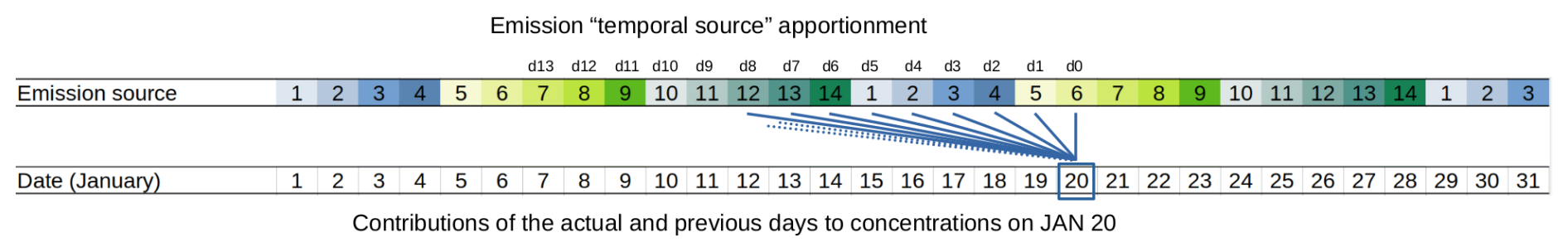
Figure 1 The concept of temporal source apportionment. Emissions are divided into 14 artificially distinguished source sectors while emissions from each sector emits exactly once in 14 d (marked with different colors). The classical PSAT technique enables to calculate the contribution of each “source sector” to a given day (20 January in this case), which further enables to calculate the contributions of the emissions from the actual (d0) and previous days (d1 to d13) to a given day's PM concentration.

In order to calculate the contributions of anthropogenic emissions from different days to a given day's daily PM concentration, we adopted the PSAT technique offered by CAMx along with tagging emissions based on the day they are emitted, leading to our approach called Temporal Source Apportionment (TSA). This means that emissions are not split into different human activity sectors (like transport, heating, etc.) and/or different geographical regions (e.g. continents, countries, etc.) like it is usually done when applying source apportionment. Instead, we split them into 14 artificial “temporal sectors” corresponding to one day within 14 d period and this means that emissions from each of these 14 “sectors” occur once in 14 d. On other days, they are exactly zero. With this, emissions are continually introduced to the system as if no temporal source apportionment was used, the only difference is the tagging of emissions according to the day they have been emitted. Figure 1 visualizes this method showing the 14 different “temporal sector” for a chosen month (January) and an example of how the contributions of emissions from different days are obtained by this approach for a chosen date (20 January in this case). The choice of 14 d comes from an estimate of the upper limit of the aerosol lifetime in the troposphere based on Seinfeld and Pandis (2016) and Kristiansen et al. (2016). Technically, this of course means that for a given day, the contribution from emissions at day minus X (where X is between 0 and 13) will, in fact, contain the contribution from day minus X+14; X+28; X+42 d and so on, however, after two weeks virtually all emissions from the domain are either deposited or advected off the domain, thus not contributing to the local concentrations. The contributions from such days in the far past can thus be disregarded. To complement the 14 anthropogenic “temporal” source sectors, we included a 15th one which contains all natural emissions, which in our case mean the biogenic emissions calculated by the MEGAN model. However, this 15th sector is relevant only for SOA and consequently for PM_2.5 and will not be analyzed for other PM components. It should also be noted that the contributions from these 15 sectors do not sum up to 100 % as one has to account for the contribution of long range transport, which manifests itself through the acting of the boundary conditions. However, in the present study, only the impact of local (i.e. falling within the domain) emissions are assessed. It has to be also added, that the mutual interaction of emissions from different days are not accounted for in the PSAT methods as it calculates the pure contributions (e.g. contribution of sulfur emissions – via SO₂ to sulfates). It, by principle, is not able to calculate the chemical impacts which contain a non-linear component (Bartík et al., 2024). To do so, one would need to remove (zero-out) emissions from each day from the cyclic 14 d period and repeat the whole 10 year CAMx simulation without these emissions which would however require 14 additional simulations. This would be however computationally extremely demanding so we decided to chose the (temporal) PSAT method.

As was mentioned above, anthropogenic emissions are from year 2015 introduced for all other simulated years; however, the meteorological conditions vary year-by-year. This means that the calculated variability of the results is caused by the variability of the meteorological conditions. Indeed, these can have a substantial impact on emissions contributions. E.g. strong vertical mixing resulting from unstable vertical stratification can cause the emissions can be transported to higher elevation making their life-time longer (before they are deposited back to the surface), or on the other hand, stable conditions with potentially elevated inversions layers resulting in limited vertical mixing cause the accumulation of emissions in the lower boundary layer which can enhance the impact of local emissions even those from past days. Additionally, temperature itself can also affect the contribution of previous days emissions: e.g. during hot summer days, elevated temperatures cause faster chemical decay of secondary aerosol components (or even their precursors) reducing their life-time, but on the other hand, convective transport resulting in heating of the earth's surface can lift PM to higher levels prolonging their lifetime because of delayed to deposition. Strong winds can also cause reduction of impact of the local actual day's emissions while these can be transported to long distances, affecting the PM pollution elsewhere already as a previous day's emission. Finally, rainy periods are responsible for fast wet removal of particulate matter, which again reduce the life-time of emissions.

3 Results

3.1 Model validation

Our model simulation with CAMx is identical to the one presented in Prieto Perez et al. (2025) in terms of the results. The one here differs only by the application of the PSAT technique which has, however, (logically) no effect on the concentrations, it only offers a new type of output data and thus more detailed insight on the contributors to the air pollution. The study mentioned above performed a very detailed validation of the CAMx model simulations (along with the WRF-Chem outputs) which included comparison of key pollutant concentrations with surface observational data (AirBase: European Air Quality Measurement stations, https://eeadmz1-downloads-webapp.azurewebsites.net/, last access: 20 March 2026) (EEA, 2023) while the validation was performed separately for urban and rural stations. For this reason, we limit this section to the most important outcomes of this comprehensive study showing the average monthly and diurnal variation of particulate matter (PM_2.5 and PM₁₀) including the main precursors of inorganic aerosol (NO₂ and SO₂).

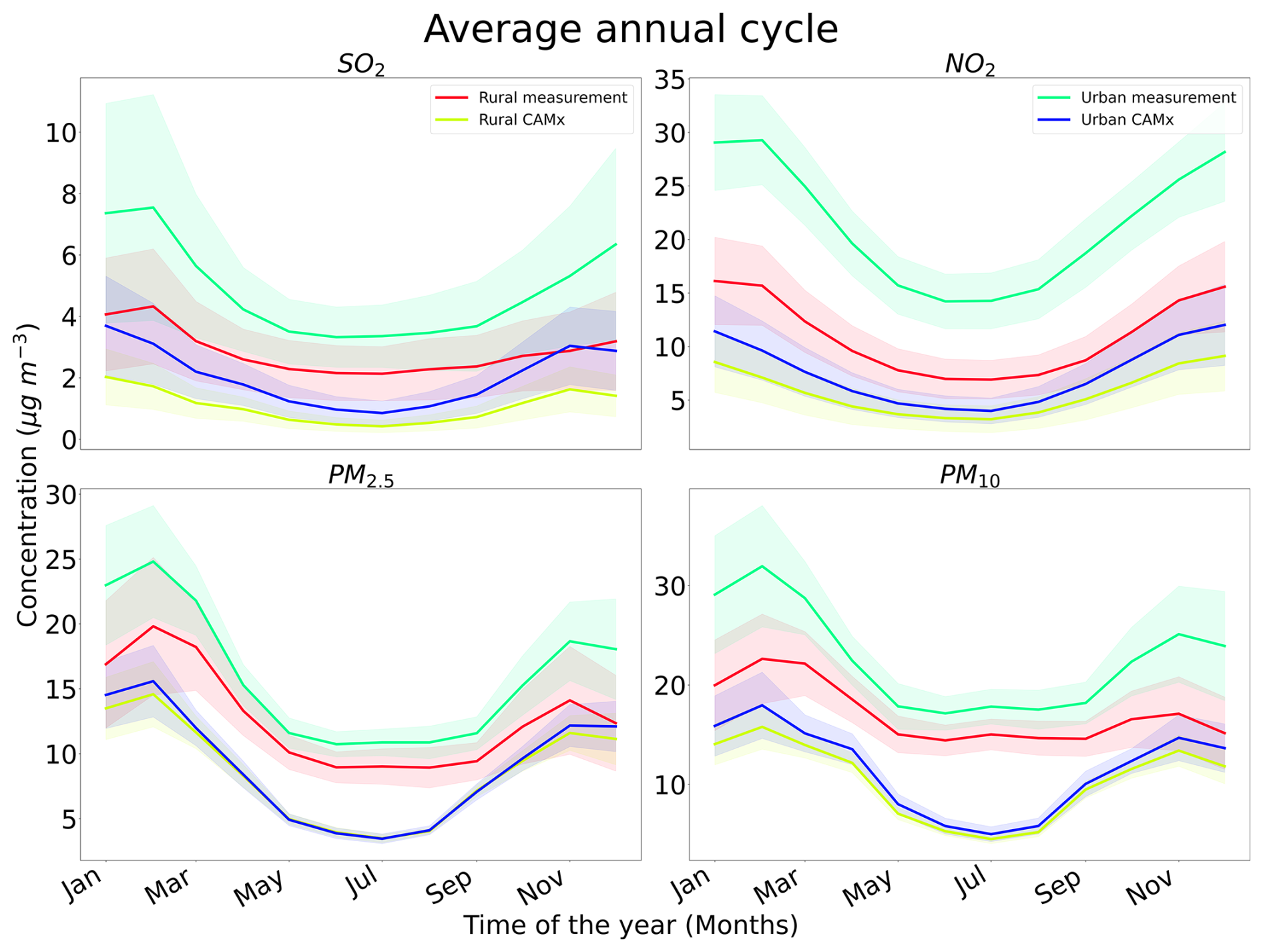
Figure 2 The comparison of 2010–2019 averaged annual cycles of monthly mean near surface concentrations of SO₂, NO₂, PM_2.5 and PM₁₀ for Airbase stations (red and green) and the corresponding series for CAMx (yellow and blue). Rural and urban stations are treated separately. The shaded areas denote the standard deviation of the mean. Units in µg m⁻³.

Figure 2 depicts the average annual cycles of monthly mean values for all four pollutants, while the standard deviation of the mean is shown by the shaded area above and below the corresponding line. For SO₂ values are, in general, strongly underestimated, especially for urban stations reaching 4 µg m⁻³ underestimation during winter and slightly less in summer (3 µg m⁻³). For rural stations, sulfur dioxide is underestimated by about 2 µg m⁻³ with slightly larger negative bias in winter. In relative numbers, CAMx predicts often about 50 % smaller concentrations and this negative bias occurs throughout all months and for both rural and urban stations.

For NO₂, underestimation prevails reaching about 3–6 µg m⁻³ for rural stations while it is larger during winter. Over urban areas the underestimation can reach values up to 15 µg m⁻³ in winter and around 10 µg m⁻³ in summer.

For PM_2.5 and PM₁₀, we also encountered a strong systematic underestimation that reached over urban stations about 10 and 10–15 µg m⁻³, respectively, while being larger in winter. Over rural stations, the negative model bias lies in the 5–10 µg m⁻³ interval and is usually larger during summer. This means that CAMx again predicts about 50 % lower concentrations compared to the measured ones.

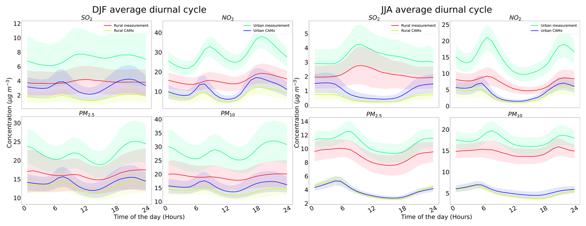
Figure 3 The comparison of 2010–2019 averaged diurnal cycles of DJF (left) and JJA (right) hourly near surface concentrations of SO₂, NO₂, PM_2.5 and PM₁₀ for Airbase stations (red and green) and the corresponding series for CAMx (yellow and blue). Rural and urban stations are treated separately. The shaded areas denote the standard deviation of the mean. Units in µg m⁻³.

To investigate how these biases evolve throughout the day, we also plotted the average DJF (December–January–February, i.e. winter) and JJA (June–July–August, i.e. summer) diurnal variation of the measured and modeled concentrations of the above-mentioned pollutants in Fig. 3 along with the standard deviation of the mean values. For SO₂ one striking feature is that the model predicts two distinct peaks for winter corresponding to the morning and evening peaks of emissions and suppressed mixing. However, this is not seen in the measured data so clearly, which indicates a maximum occurring rather later and a smaller secondary maximum too. This leads to a maximal bias over urban areas during noon of about 6 µg m⁻³. For JJA, measured values predict one maximum for both rural and urban stations which is not resolved by CAMx leading to the maximum of the negative biases occurring during daytime reaching 3 µg m⁻³. CAMx is somewhat more successful in resolving the diurnal cycle for NO₂ with aligning maxima of both measured and modeled concentrations occurring during morning rush hours and early evening hours (being very similar to modeled SO₂ diurnal cycles). The underestimation, however, remains the same during the day and in both seasons while it is larger (as expected) for urban stations (about 10 µg m⁻³ during morning rush hours). Finally, winter PM exhibits two modeled peaks similar to SO₂ and NO₂ while these peaks are also present in the measured concentrations, although the morning peak occurs later in the measured data enhancing the model negative bias (around 15 µg m⁻³).

In general, CAMx exhibits a clear underestimation of the measured pollutant concentrations for both the gas-phase precursor species and PM, especially over urban areas. Prieto Perez et al. (2025) offers a more detailed insight in the potential causes of this negative bias, mentioning the overestimated vertical mixing in driving meteorological data and generally underestimated emissions estimates as the main cause, while incorrect hourly disaggregation factors describing the diurnal variation of the different activity sources also play a role. The underestimation of emissions follows also from the emission evolution figure in Fig. S1 where it seen that the 2015 emission is rather below the 2010–2018 average (2019 was missing from CAMS data) due to very high reported emissions for years 2010–2014. Due to this underestimation of PM, we can expect that the contributions of previous days emissions presented in the next sections will be also correspondingly underestimated. However, the relative contributions are probably not affected considerably, as they are calculated from the total concentrations too.

3.2 Impact of emissions from previous days

This section presents the spatial impacts of emissions from different days, while the variability of the impact will also be presented. Due to a very rapid decrease of the contribution of emissions from previous days (as going more into past), for PM_2.5 only the impacts until day-6 will be shown, while for its components, we will show only the contribution until day-5. Moreover, as BVOC emissions are relevant for SOA and thus PM_2.5, we will include their contribution in case of these only.

3.2.1 Spatial patterns of the impact

In Fig. 4, the absolute and relative impacts on winter (DJF) PM_2.5 near surface concentrations are presented. The impact of the actual day's emissions (day-0) reaches about 10–15 µg m⁻³ above central Europe and northern Italy while other areas encounter values about 4–6 µg m⁻³. These numbers correspond to a relative contribution of 40 %–60 %. From the previous day, the impact reaches slightly lower values (up to 10 µg m⁻³), except Italy, where it can be as high as 15 µg m⁻³. In relative numbers, this makes about 30 %–50 % contribution. For emissions from day-2 and day-3, the impact decreases over central Europe to values of up to 2 and 0.4–0.8 µg m⁻³ (5 %–10 % and 2 %–5 %), respectively, while again over northern Italy they remain higher, reaching 4–6 µg m⁻³ (about 5 %–10 %). When going even further to the past (day-4 to day-6), the impacts become significantly smaller, while the highest values are reached over Italy, up to 1, 0.8 and 0.2  µg m⁻³ (5 %, 1 % and 0.5 %) for day-4 to day-6, respectively. Over other areas, the relative contributions are even lower. Finally, the contribution from biogenic emissions to winter PM_2.5 concentrations is 0.1–0.4 µg m⁻³ which is about 1 %–5 %, and was expected to be low in this season.

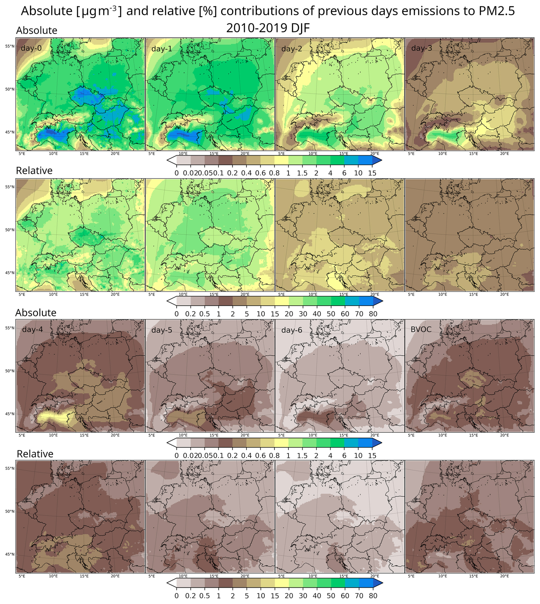
Figure 4 The absolute (1st and 3rd row) and relative (2nd and 4th row) contributions of emissions of the actual and previous days as well as from biogenic emissions to the 2010–2019 DJF average near surface PM_2.5 concentrations. Upper two rows present the contribution from the actual (day-0) and the three previous days (day-1 to day-3), while the lower two rows show the same for day-4 down to day-6 and for the biogenic emissions. Units are µg m⁻³ for the absolute and % for the relative contributions.

During summer (JJA), Fig. 5, impact of the actual day's emissions reaches about 1–6 µg m⁻³ over norther Italy and Germany (corresponding about 20 %–30 % relative contribution), while over other areas the contribution is about 0.2–1 µg m⁻³ that corresponds to 15 %–30 %. From the previous day, the impact reaches 0.2 µg m⁻³ (5 %) over large areas while it is about 0.4–0.6 µg m⁻³ (up to 10 %) over Italy. For emissions from day-2 and day-3, the contributions reach 0.2 µg m⁻³ over northern Italy, but remain under 0.1 µg m⁻³ over other areas with relative contributions up to 5 % and 2 % for day-2 and day-3, respectively. For day-4 to day-6, the contributions become negligibly small and these results are included in the Supplement as Fig. S2 (along with the day-0 to day-3 contributions as well). As for the contribution of BVOC emissions, it is larger than in DJF, as expected, and reaches 0.5 µg m⁻³ (while being almost 0.8 µg m⁻³ over many areas). This is about 10 %–30 % in relative numbers.

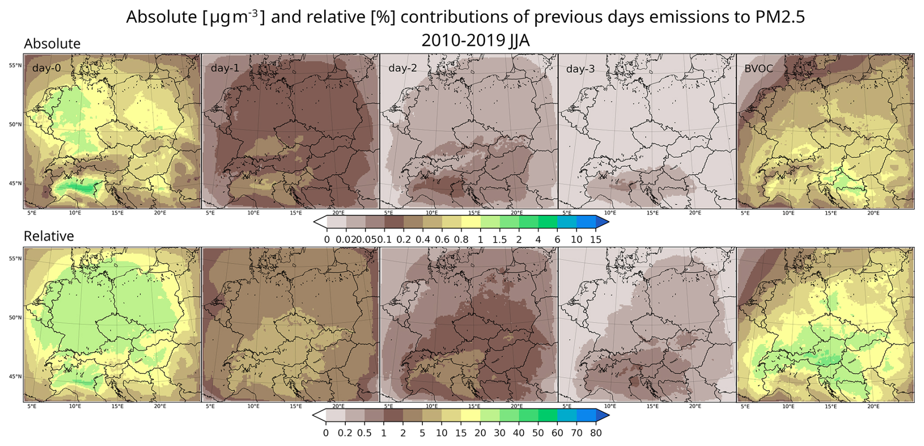
Figure 5 The absolute (upper row) and relative (lower row) contributions of emissions of the actual and previous days (day-0 to day-3) as well as from biogenic emissions to the 2010–2019 JJA average near surface PM_2.5 concentrations. Units are µg m⁻³ for the absolute and % for the relative contributions. For the contributions of older emissions, see Fig. S2 in the Supplement.

Figures S3–S6 show the impacts (both absolute and relative) for PM_2.5 above but for individual years. It is clear that the year-to-year variability is rather small, and the pattern calculated from the 10 year average resembles the pattern obtained for individual years, for both summer and winter.

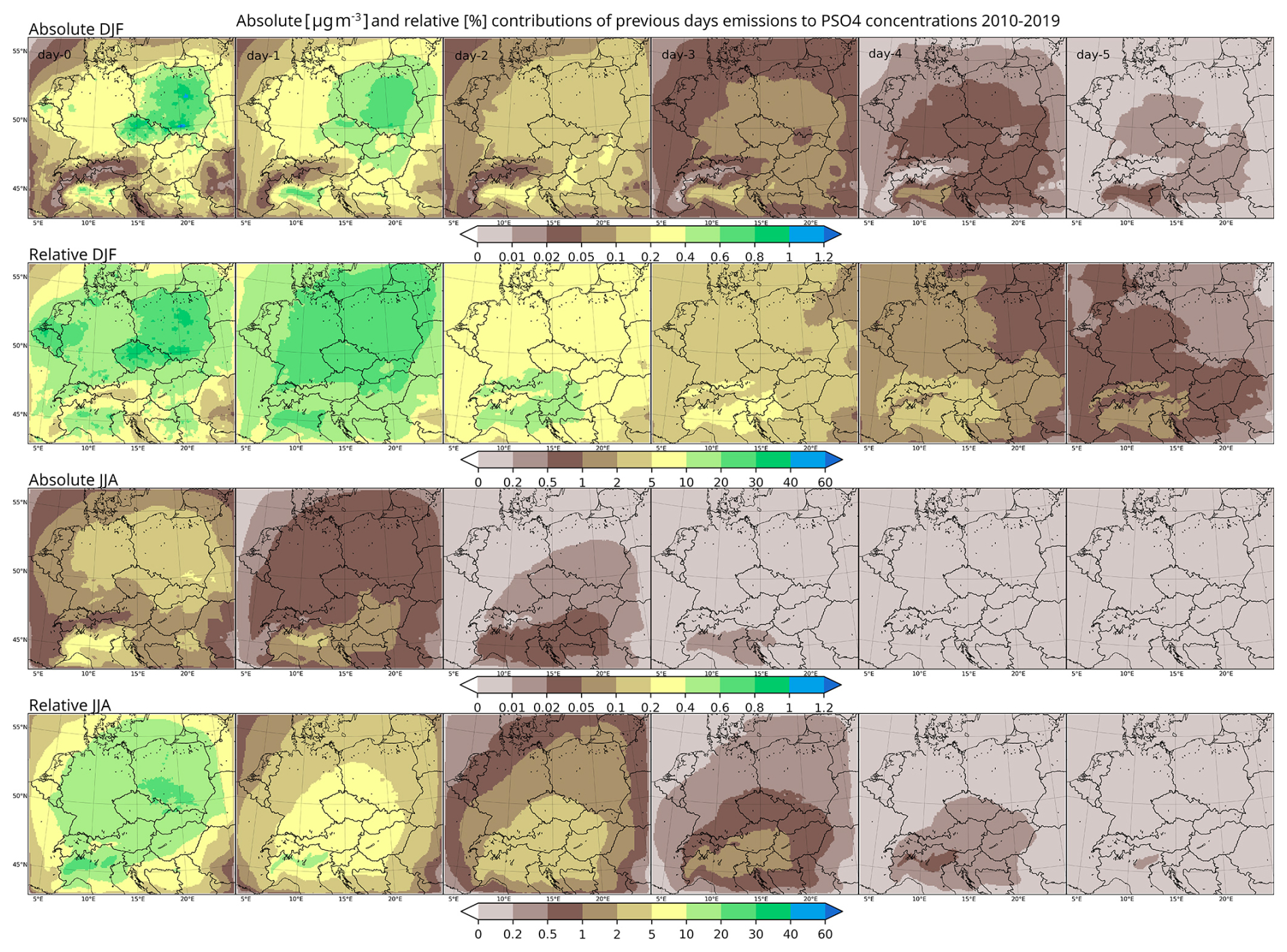
Figure 6 The absolute (1st and 3rd row) and relative (2nd and 4th row) contributions of emissions of the actual and previous days emissions to the 2010–2019 DJF and JJA (upper two and lower two rows, respectively) average near surface sulfate (PSO₄) concentrations. Columns stand, from left to right, for the contribution of the actual day (day-0) and previous days (day-1 to day-5). Units are µg m⁻³ for the absolute and % for the relative contributions.

In further, the individual components of the fine PM and the contribution of previous days' emissions to their concentration will be examined, starting with the secondary inorganic aerosol (sulfates – PSO₄, nitrates – PNO₃ and ammonium – PNH₄), then looking at secondary organic aerosol (SOA) and finally to primary organic aerosol (POA) and primary elemental carbon (PEC). Figure 6 shows the absolute and relative contributions of actual and previous days (day-1 to day-5) emissions to both winter and summer near-surface concentrations of PSO₄. In DJF, the contribution from day-0 and day-1 emissions is about 0.4–1 µg m⁻³, especially above central Europe and northern Italy, which corresponds to about 20 %–40 % relative contribution to absolute sulfate concentrations. For day-2 and day-3, the contribution decreases to 0.4 and 0.2 µg m⁻³ (20 % and 10 %), respectively. Going even further to the past (day-4 and day-5), the contribution becomes very small, usually below 0.1 µg m⁻³ (1 %–2 %). During JJA, when fewer sulfates are usually formed, the contributions are generally lower. For emissions from day-0 and day-1, they are about 0.1–0.4 µg m⁻³ at most, corresponding to 5 %–20 % relative contribution, while for other days in the past (day-2 and day-3) it becomes even smaller, below 0.05 µg m⁻³ (2 %). From day-4 and day-5 the contributions become negligible, usually below 0.5 %.

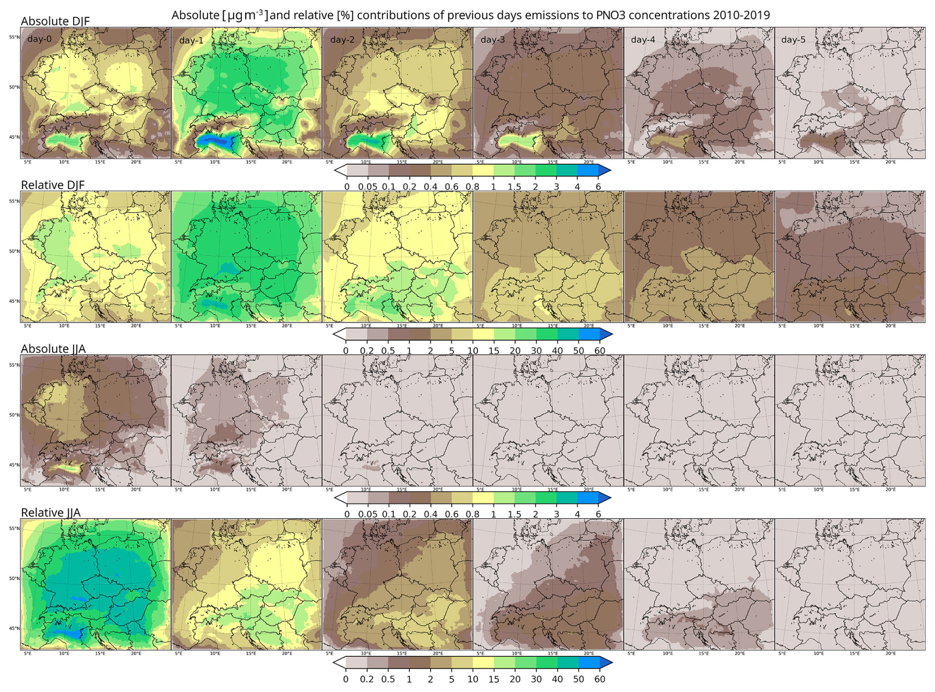
Figure 7 Same as Fig. 6 but for particulate nitrates (PNO₃).

Similarly to PSO₄, Fig. 7 shows the absolute and relative contributions of the actual and previous days' emissions to both winter and summer near-surface concentrations of PNO₃. In DJF, the contribution from the actual day's emissions is about 0.6–2 µg m⁻³, highest above northern Italy, corresponding to about 10 %–20 % relative contribution to the absolute nitrate concentrations. Surprisingly, the contributions of emissions from day-1 are higher and can reach 4–6 µg m⁻³ over northern Italy, while being above 2 µg m⁻³ over central Europe. This corresponds to relative contribution of about 20 %–40 %. For day-2 and day-3, the contributions reach 0.4 and 1 µg m⁻³ (5 %–20 %) over central Europe, while about 3 and 1.5 µg m⁻³ (5 %–30 %) over northern Italy. For emissions from day-4 and day-5, the contribution decreases to less than 0.2 µg m⁻³ (less than 0.8 µg m⁻³ over northern Italy) with relative contributions below 5 % and 2 %, respectively. During summer, when nitrate formation is much more suppressed, the contributions are significant only for day-0 to day-3, being below 1.5 µg m⁻³ over northern Italy, but usually even lower (up to 0.5 µg m⁻³) over other parts of the domain. This corresponds to relative contribution about 40 %–50 % and 10 %–20 % for day-0 and day-1 while for day-2 and day-3, the relative contributions are below 10 % and 2 %, respectively. Finally, for day-4 and day-5, the absolute contributions remain below 0.05 µg m⁻³ (below 0.5 %).

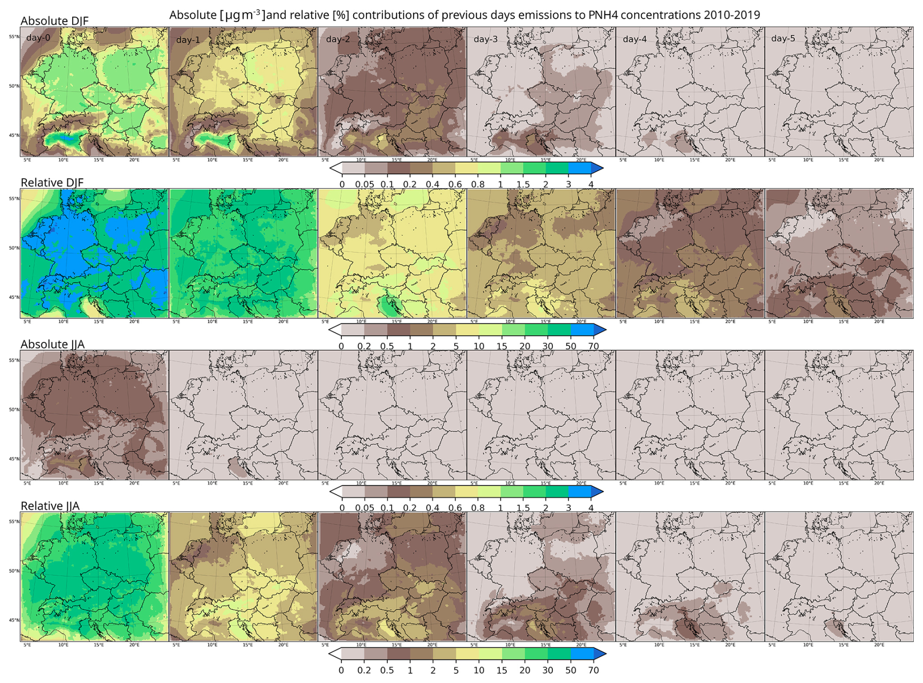
Figure 8 Same as Fig. 6 but for particulate ammonium (PNH₄).

Figure 8 shows the absolute and relative contributions of the actual and previous days (again, day-0 to day-5) emissions to both winter and summer near-surface concentrations of PNH₄. In DJF, the contribution from day-0 and day-1 emissions is approximately 1–4 µg m⁻³, especially above central Europe and northern Italy, which corresponds to about 20 %–70 % relative contribution to absolute ammonium concentrations. For day-2 and day-3, the contribution goes below 0.6 and 0.2 µg m⁻³ (10 % and 5 %), respectively. Going even further to the past (day-4 and day-5), the contribution becomes very small, usually below 0.05 µg m⁻³ (2 %). During JJA, less ammonium is usually formed and the contributions are generally lower. For emissions from day-0 and day-1, they are about 0.05–0.4 µg m⁻³ at most, corresponding to 5 %–20 % relative contribution, while for other days in the past (day-2 and day-3) it becomes even smaller, below 0.05 µg m⁻³ (below 5 %). From day-4 and day-5 the contributions become negligible, usually below 0.2 %. For a detailed explanation of the rapid ammonium decrease refer to the discussion section.

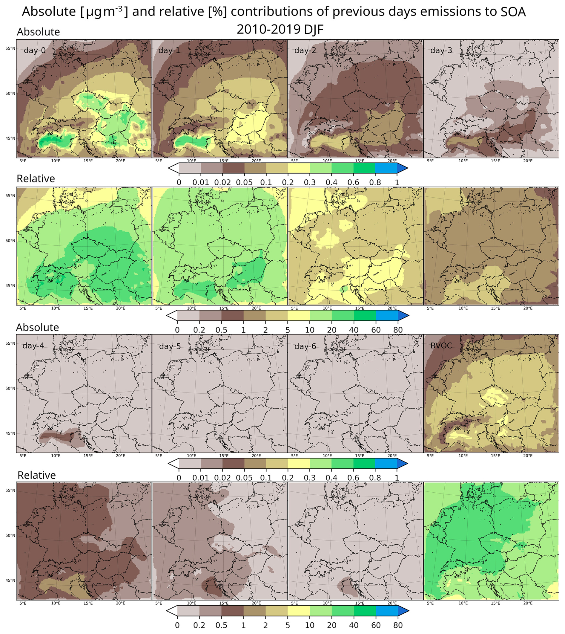
Figure 9 The absolute (1st and 3rd row) and relative (2nd and 4th row) contributions of emissions of the actual and previous days as well as from biogenic emissions to the 2010–2019 DJF average near surface SOA concentrations. Upper two rows present the contribution from the actual (day-0) and the three previous days (day-1 to day-3), while the lower two rows show the same for day-4 down to day-6 and for the biogenic emissions. Units are µg m⁻³ for the absolute and % for the relative contributions.

In case of secondary organic aerosol, in addition to anthropogenic emissions, one has to consider also the contribution from biogenic sources; therefore we present the spatial figure in the same manner as for PM_2.5, and distinguish between the DJF and JJA impact. In case of DJF (Fig. 9), the absolute impact of emissions from day-0 and day-1 reaches 0.2–0.6 µg m⁻³ over central Europe and northern Italy which corresponds to about 10 %–40 % relative contribution. For day-2 and day-3 emissions, the contribution becomes usually less than 5 % and 2 %, respectively, while for even further past (day-4 to day-6), the relative contribution is less than 1 % (but usually even less than 0.5 %). The contributions of BVOCs are somewhat larger, around 10 %–40 % which is comparable to the contribution from emissions from day-0 and day-1.

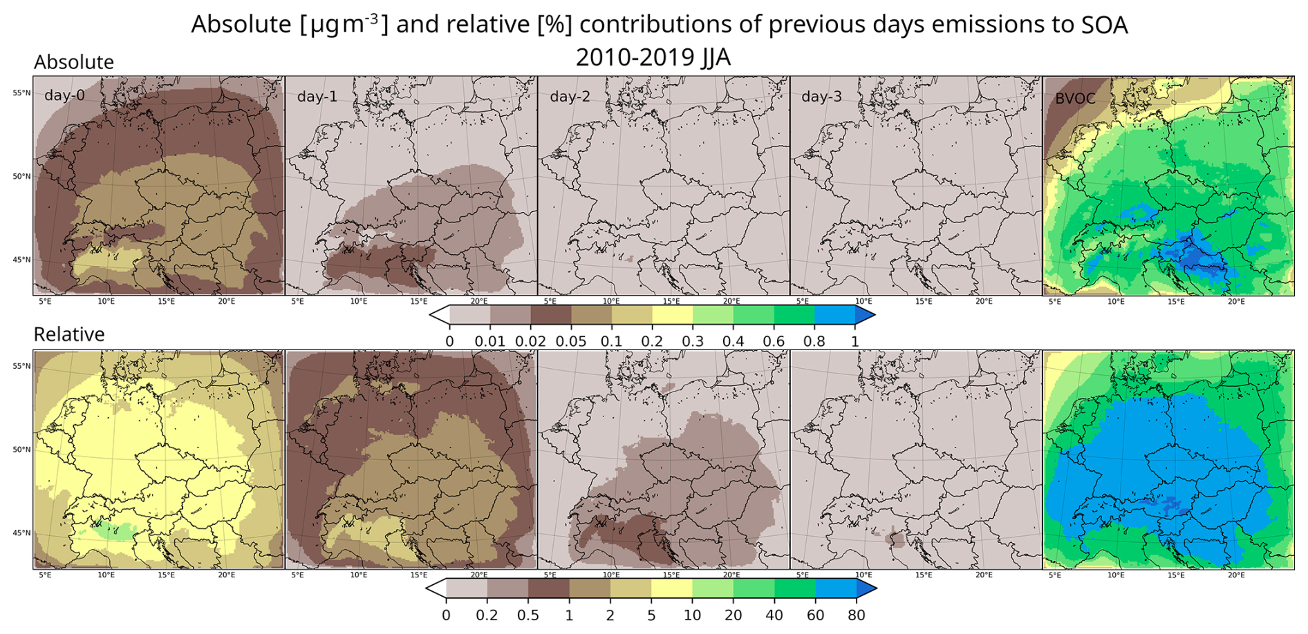
Figure 10 Same as Fig. 9 but for JJA and showing only the day-0 to day-3 emission contributions (both absolute and relative). The contributions from older emissions are depicted in Fig. S8 in the Supplement.

During JJA (Figs. 10 and S8), the absolute impact of emissions from day-0 and day-1 on SOA reaches 0.05–0.2 µg m⁻³ over central Europe and northern Italy which corresponds to about 2 %–10 % contribution. For day-2 and day-3 emissions, the contribution usually decreases to less than 1 % and 0.5 %, respectively, while for even further past (day-4 to day-6), the relative contribution is less than 0.2 % (Fig. S8). The contribution of BVOC emissions is, however, large, reaching 1  µg m⁻³, or 60 %–80 % in relative numbers. In other words, the majority of SOA is produced from biogenic emissions over the region in focus.

Figure 11 Same as Fig. 6 but for primary organic aerosol (POA).

Finally, we will look at the impact on the two important primary components of the total PM_2.5, the POA and PEC. Figure 11 shows the absolute and relative contributions of actual and previous days (day-0 to day-5) emissions to both winter and summer near-surface concentrations of primary organic aerosol. In DJF, the contribution of day-0 and day-1 emissions can reach about 1 to 6 µg m⁻³, especially above central Europe and northern Italy, that corresponds to about 30 %–60 % relative contribution to absolute ammonium concentrations. For day-2 and day-3 emissions, the contribution usually goes below 0.5 and 0.1 µg m⁻³ (10 % and 5 %), respectively. Going even further into the past (day-4 and day-5 emissions), the contribution becomes very small, usually below 0.05 µg m⁻³ (up to 2 % relative contribution). During JJA the contributions are generally lower. For emissions from day-0 and day-1, they are about 0.05–0.2 µg m⁻³ at most, corresponding to 5 %–20 % relative contribution, while for other days in the past (day-2 and day-3) it becomes even smaller, below 0.02 µg m⁻³ (less than 5 %). From day-4 and day-5 the contributions become negligible, usually below 0.2 % in relative numbers.

Due to large similarities to POA results, the absolute and relative contributions of the actual and previous days emissions to PEC concentrations are presented in the Supplement in Fig. S7. During winter, the contribution from day-0 emissions reach 2 µg m⁻³ over central Europe and can be even greater over northern Italy, up to 4 µg m⁻³ (around 50 %–70 %). The contribution of day-1 emissions is about 0.2–0.4 and up to 1 µg m⁻³ over central Europe and northern Italy, making it about 15 %–20 % relative contribution. For day-2 and day-3 emissions, the contribution goes below 0.2 µg m⁻³ (10 % in relative numbers) and for day-4 and day-5 emissions, the contribution remains less than 2 %, but usually even less than 1 %. During summer, day-0 and day-1 emissions contribute by up to about 0.1 and 0.05 µg m⁻³, respectively, making around 30 %–50 % and 5 %–15 %, respectively. For day-2 and day-3 emissions, the contributions usually remain below 0.01 µg m⁻³ (up to 5 %) while for day-4 and day-5 emissions, the relative contributions are below 1 % or usually even below 0.5 %.

From Figs. 4 to 11 we saw that while the absolute contribution of emissions from different days differ greatly by geographical location, the relative contributions have lower spatial variability. To confirm this, we plot in Fig. 12 the relative contributions of emissions from different days for the centres of selected large urban areas over the domain in focus (namely Berlin, Budapest, Milan, Munich, Prague, Vienna and Warsaw). In general, the figure shows that the contribution decreases with the time lag of the emissions with some exceptions for day-1 (previous day emissions, e.g. for sulfates and nitrates) which will be detailed below.

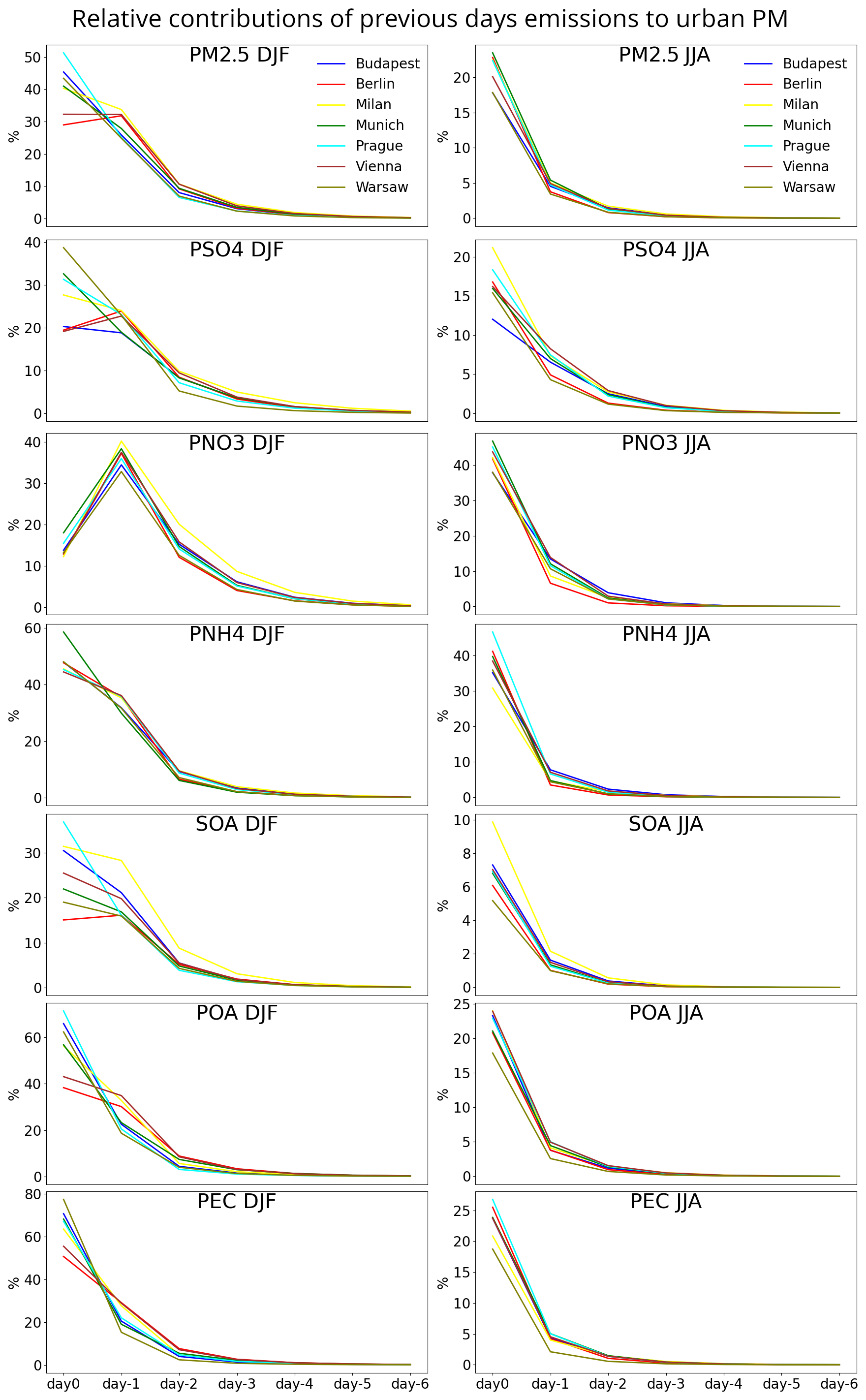
Figure 12 The relative contribution of day-0 to day-6 emissions to DJF (left) and JJA (right) urban concentrations of PM_2.5 and their components (PSO₄, PNO₃, PNH₄, SOA, POA and PEC). The data are taken from model gridboxes covering the city centers of Budapest, Berlin, Milan, Munich, Prague, Vienna and Warsaw. Units are in %.

For total PM_2.5, contributions start (for day-0) at around 30 %–50 % and around 20 % for winter and summer, respectively. Then they go to 30 % and 5 % for day-1, and 10 % and below 5 % for day-2. For some of the cities in winter (Berlin and Vienna), the contribution to PM_2.5 from day-0 and day-1 is very similar, pointing out the importance of emissions that were released on previous days and probably highlighting the fact of reduced dispersion during DJF. For sulfates, the relative contributions for the day-0 emissions are, however, much more variable between cities in DJF, ranging from about 20 % to 40 % while in JJA, they are around 12 %–17 %. For day-1, the contributions go to 20 % and 5 %–10 %, respectively, while for day-2, they get below 10 % and 5 % for DJF and JJA. It can also be seen that contribution to sulfate concentrations can be higher for day-1 for some cities (Berlin and Vienna), probably in connection with limited dispersion but also due to some time sulfates require to be formed.

For nitrates, a very striking feature is evident (also seen in the spatial figure Fig. 7). While the winter day-0 contribution is around 15 % for each city, the day-1 contribution significantly increases to 30 %–40 % (for each city) and they for day-2 and day-3, it goes again down to 15 % and below 10 %. This is not seen in summer where the relative contributions for day-0, day-1 and day-2 are continually decreasing from around 40 % to 10 % and 5 %. Here, the probably reason for this behavior is that during winter, when nitrates usually form, the oxidation takes some time and will take place in aged plumes rather than in “fresh” ones. In case of ammonium, the contribution of day-0 emissions is between 40 %–60 % and 35 %–45 % during DJF and JJA, respectively. For day-1 emissions, it is slightly below 40 % and below 10 % for the two seasons, while for day-2 it goes further down below 10 % and 5 %.

The contributions for SOA have a large spread for day-0 emissions during winter, ranging from 15 % to 35 %, while in summer they are smaller around 5 %–7 %. For day-1 emissions, the contribution is around 15 %–25 % for DJF and only 2 % for JJA, respectively. For day-2 emission, the contribution goes below 10 % and 3 % during DJF and JJA. In case of primary organic aerosol, the day-0 contributions are from 40 % to 65 % in DJF while around 20 %–25 % in JJA. For day-1 emissions, the contributions are round 20 %–30 % and 5 % during DJF and JJA, respectively, while for emissions from day-2, they are less than 10 % and 3 %. Finally, for primary elemental carbon, the contributions from day-0 emission are about 50 %–70 % and 20 %–25 % for DJF and JJA, while for day-1 emissions, they are about 20 %–30 % and 5 %, respectively. For day-2 and further into the past, they become less than 10 % and 2 % for winter and summer, respectively.

3.2.2 Variability of the daily impacts

So far, the seasonally averaged contributions (both absolute and relative) for the emissions from different days were presented. However, no information on the spread of the impact of previous days' emissions on a given day concentrations is provided. We saw in Fig. 12 that on average the contributions of emissions from day-4 to day-6 are negligible. However, can there be some circumstances when such emissions become significant for a particulate day? Here we therefore present the annual variation of the daily impact of emissions from past days in order to obtain an estimate about the possible extremes of this contribution. It has to be noted that as emissions correspond to a single year (2015) and are not varying from year to year, the variability seen here is probably the result of varying meteorological conditions that are based on a continuous 10-year model simulations (WRF).

The results are presented in Fig. 13. It is clear from the first sight that the contributions presented above represent only a 10 year average, and these can be much larger for individual days. For the winter contribution of emissions from day-0, these can reach almost 100 % (Milan), while in case of other cities, they can reach 80 %. For summer, emissions from day-0 can often reach 50 %. Emissions from day-1 can go as high as 50 %–60 % in DJF while in JJA they sometimes reach 30 %. For emissions from day-2, these can go up to 30 % in winter, while the highest values in summer are around 20 %. The day-3 emissions can also contribute by up to 20 %. For even older emissions, the maximum contributions are of order of 1 %–10 %. Specifically, for day-4 and day-5 emissions, they can reach 8 %–10 % (mostly during winter). For day-6 and day-7 emissions, these generally remain under 4 % (2 % for the day-7 emissions). We can thus conclude that occasionally the contribution of even 1 week old emissions can be significant and reach 1 %–2 %, i.e. considerably more than seen on the average figures earlier. Note that an abrupt decrease of the contribution of anthropogenic emissions in April is seen basically for each city. This is connected to the monthly time factors used for temporal disaggregation which are the same for the entire domain, and we expect that domestic combustion decreases significantly during this period making the local emissions contribution very weak (see the discussion for more details). To complement the picture about the range and distribution of impacts, we plotted in Figure S11 the boxplots of the DJF and JJA daily impact for PM_2.5 for the individual cities and for emissions from day-0 to day-7. They allow for easy comparison between the mean impact and extremes. It is seen that the means, especially in the case of older emissions and mostly in summer, are totally negligible compared to the extremes.

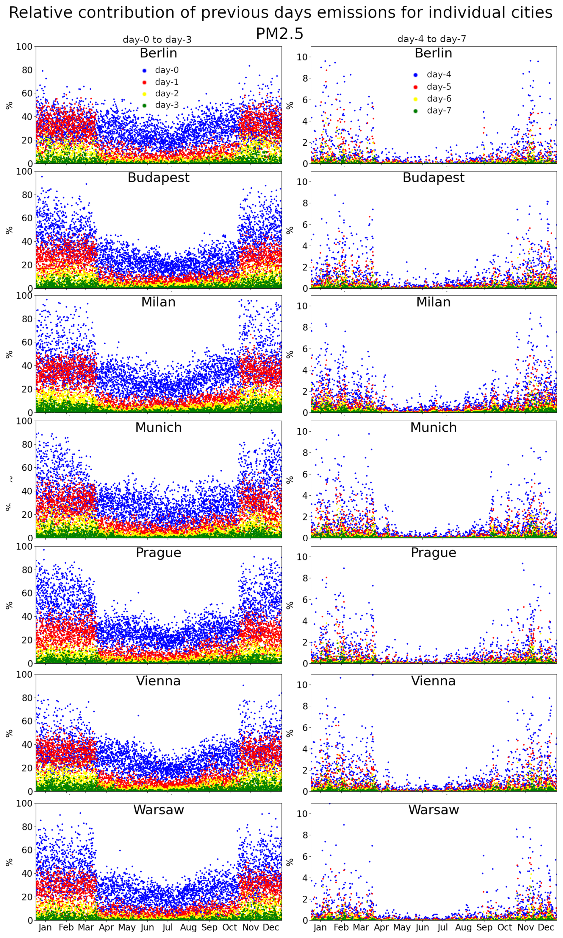
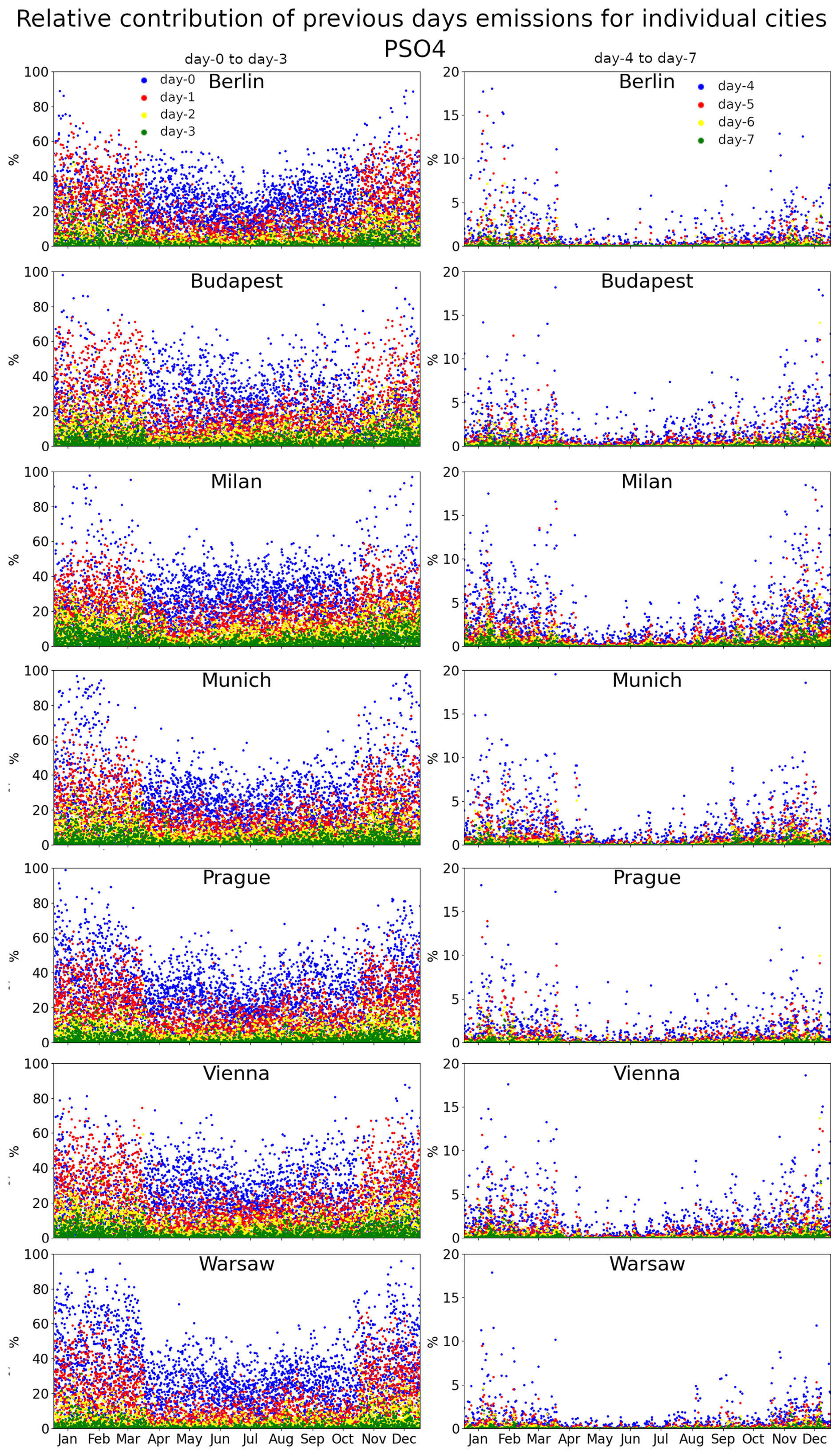
Figure 13 The relative contribution of emissions from day-0, day-1, day-2 and day-3 (left column) and emission from day-4, day-5, day-6 and day-7 (right column) to PM_2.5 concentrations for individual days from the 2010–2019 period (grouped by date in the year) for the selected cities. The blue, red, yellow and green color stand for contributions from day-0, day-1, day-2 and day-3, or from day-4, day-5, day-6 and day-7 emissions, respectively.

In addition, we also look at the variability of the impact of previous days' emissions on individual PM components. Starting with PSO₄ in Fig. 14, the contribution from day-0 can reach 90 %–100 %, especially during winter (e.g. over Munich and Warsaw), while for day-1 emissions, the contribution reaches about 70 % for some days in winter. The contribution from day-2 and day-3 emissions can be as high as 40 %–50 % and 20 %, respectively. In general, the summer values are about half of those in winter, which is again connected by the much lower local emissions over cities (related to the lack of domestic heating emissions). Regarding the contribution of even older emissions, for day-4 they can reach almost 20 % while for day-5 and day-6, they often get as high as 15 % and 5 %, respectively. Finally, for one week old emissions (day-7), the contribution can be still significant for some days, about 3 %–4 %.

Figure 14 Same as Fig. 13 but for sulfates (PSO₄).

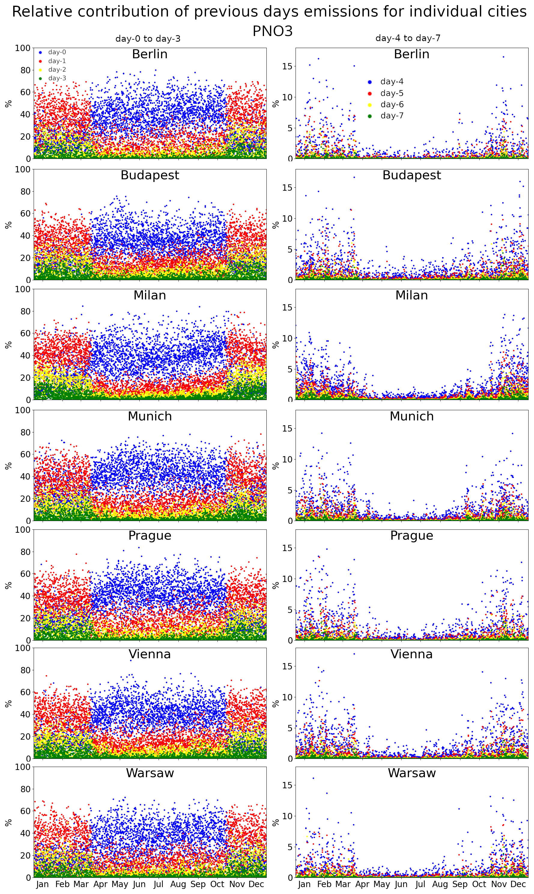
For PNO₃ (Fig. 15), the contribution from day-0 can reach about 50 %–60 % in winter, while during summer it can go even up to 70 %–80 %. In line with the average contribution figures above, the day-1 emissions have a higher contribution during winter than the emissions from the actual day, making around 60 %–80 % contribution. Emission from day-2 and day-3 can contribute by as much as 40 % and 20 % (mainly during winter). For emissions from day-4 and day-5, the contributions can reach 15 % and 10 % (again mostly during winter), while for emissions from day-6 and day-7, they are at most around 5 and 2 %–3 %, respectively, so one week old emissions can still be significant.

Figure 15 Same as Fig. 13 but for nitrates (PNO₃).

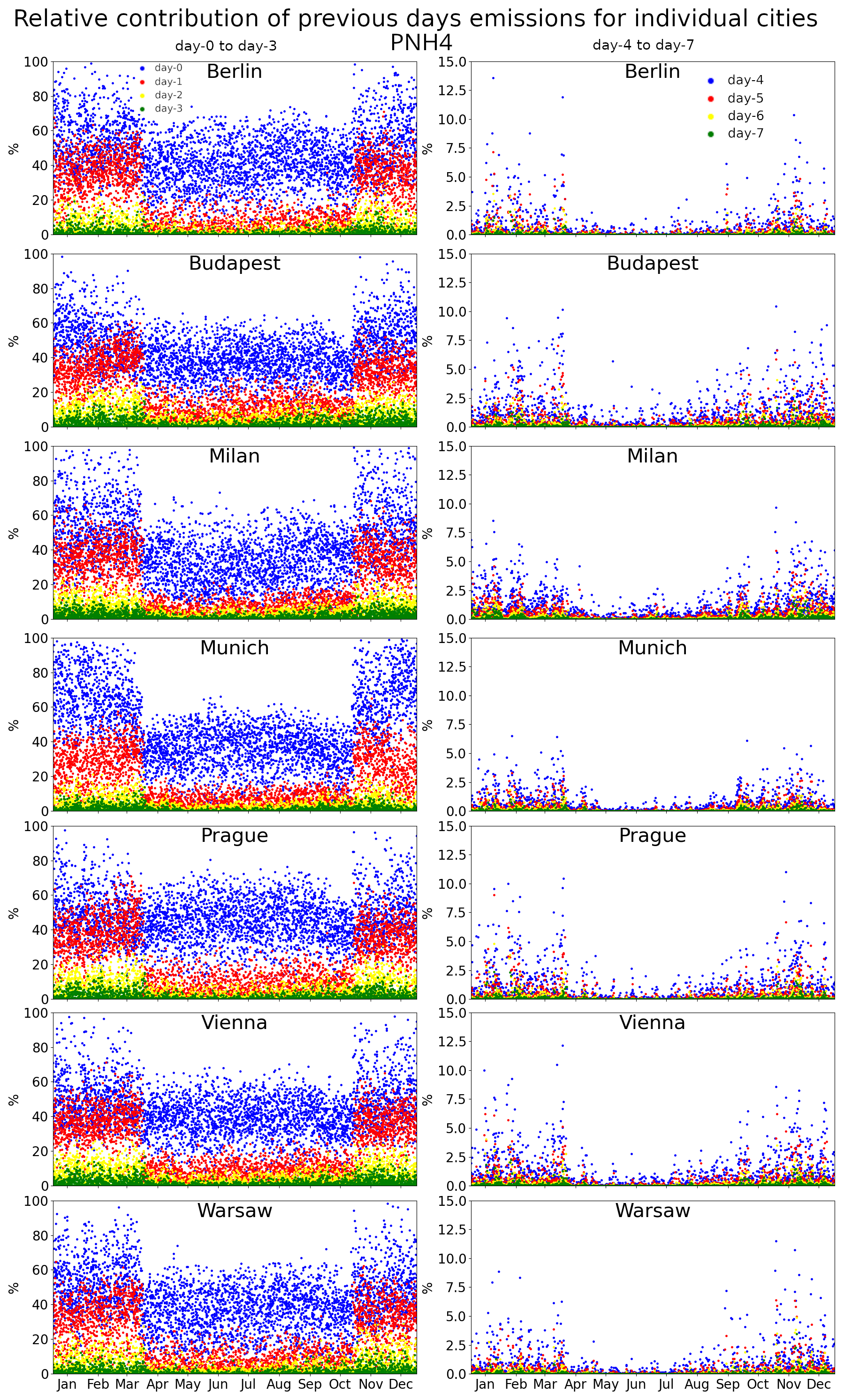
For PNH₄, presented in Fig. 16, the contribution from day-0 emissions can reach almost 100 % in winter, while during the warm season it can reach 70 %. For emissions from day-1 and day-2, it can reach an almost 70 % and 30 % contribution (also mostly during winter), while the emissions from day-3 can add about 20 %. Looking at older emissions, from day-4 and day-5, they contribute by about 12 % and 6 % at most, while for emissions from day-6 and day-7, this is not more than 2.5 % and 1 %, respectively.

Figure 16 Same as Fig. 13 but for ammonium (PNH₄).

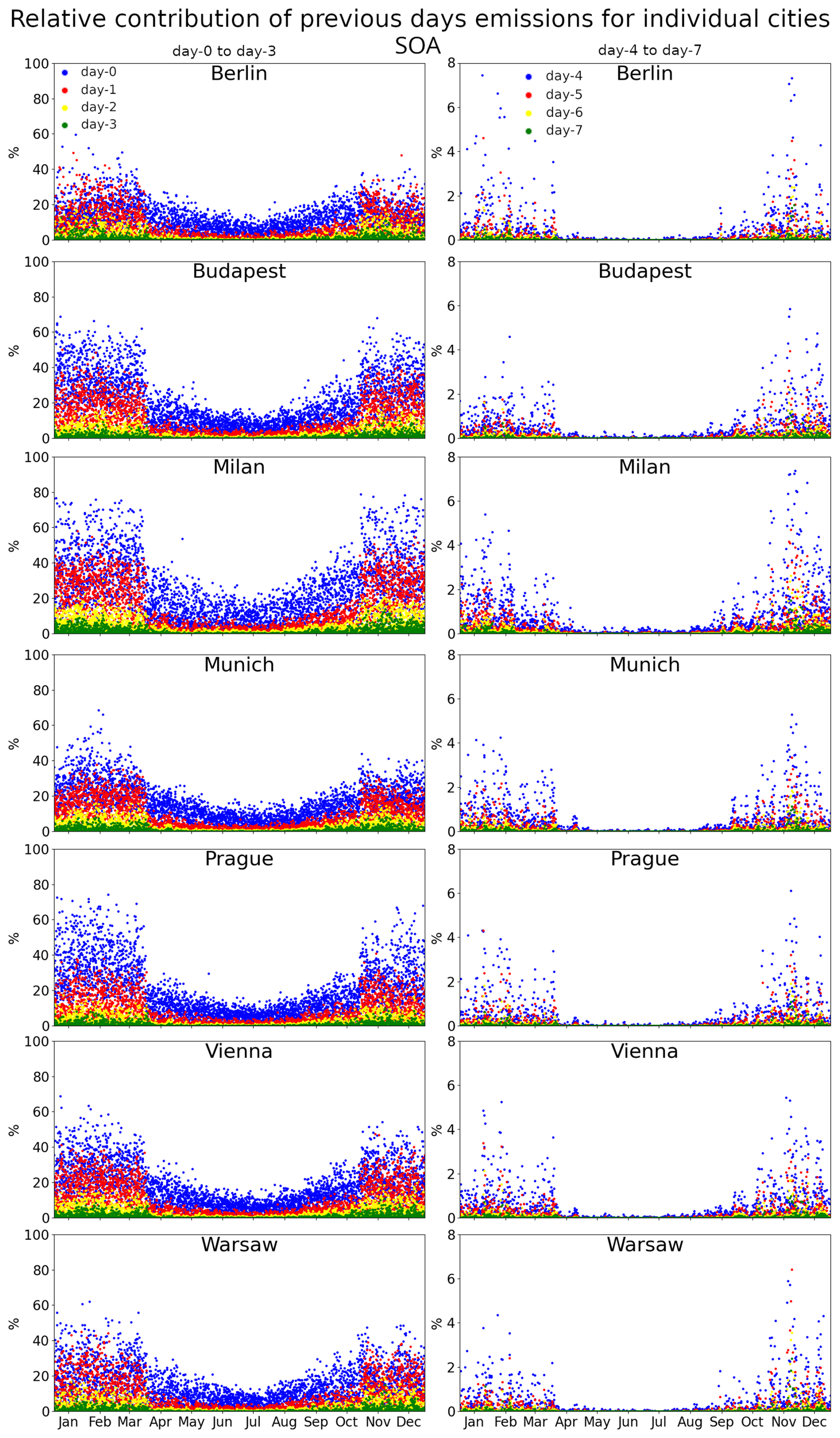
In case of SOA, Fig. 17, the actual day's emissions contribute by up to 80 % (reached over Milan), mostly during winter (in summer, it goes up to 30 % only). The day-1 contribution reaches 50 % (again during winter) while the day-2 and day-3 emissions add about 20 % and 10 %, respectively. Older emissions from day-4 and day-5 contribute by up to 7 %–8 % and 4 %, respectively. Finally, emissions from day-6 and day-7 can add to the daily concentrations as much as 1 % (only during winter).

Figure 17 Same as Fig. 13 but for secondary organic aerosol (SOA).

The daily contributions to POA and PEC concentrations exhibit similar patterns and are comparable to PM_2.5, therefore these are presented in the Supplement as Figs. S9 and S10, respectively. For POA, actual day's emissions (day-0) can reach 100 % for winter, while during the warm season, it often reaches 50 %. The day-1 emissions contribute by up to 60 % (in DJF), while emissions from day-2 and day-3 add at most about 30 % and 15 %, respectively (again, the winter relative contributions are much higher). Older emissions, i.e. those from day-4 and day-5 contribute to POA concentrations by 10 % and up to 8 %. The contribution of day-6 emissions can be as high as 4 %. Finally, one week old emissions (day-7) can add up to 2 % to POA concentrations. For the actual day's emissions, contribution to PEC can reach 100 % for winter, while during the warm season, it often reaches 50 %. The day-1 emissions contribute up to 60 % in DJF and about 20 % in JJA, while emissions from day-2 and day-3 add at most about 30 % and 15 %, respectively (again, the relative contributions in winter are much higher). Emission from day-4 and day-5 contribute by 10 % and 8 %, similar to those for POA, while emissions from day-6 and day-7 contribute by up to about 4 % and 2 %.

We have seen that occasionally, the contribution from emissions emitted several days ago can significantly contribute, by up to a few 10 % and even one week old emissions can sometimes make a few percent. Moreover, it is also seen that the actual day's emissions form most of the concentrations during the cold part of the year, while anthropogenic emissions, in general, have a much smaller contribution during the warm season (see the Discussion for more details).

4 Discussion

The study addressed the absolute and relative role of emissions from previous days on the actual day's PM_2.5 pollution, including the quantification of these contributions to aerosol components, both primary and secondary. It showed that the contribution of previous emissions to PM_2.5 concentrations gradually decreases by days reaching negligible values after approximately 7 d on average. This is in line with the average lifetime of both the directly emitted aerosol and their precursors. Indeed, Kristiansen et al. (2016) based on global model simulations reported for the accumulation mode aerosol (corresponding to our PM_2.5) lifetimes about 9 d on average, although they also pointed out some underestimation by the models given by the strong initial removal. For black carbon which is a major component of the primary aerosol, Cape et al. (2012) and Lund et al. (2018) provided also similar estimates (about 4–12 d). Another major component of the directly emitted aerosol is the primary organic aerosol, which normally undergoes some oxidation Goel et al. (2024) however, in CAMx version 7.20 it is not oxidized and behaves like inert material, therefore has probably an overestimated model lifetime. Thus contributions of previous days' emissions to POA could be somewhat overestimated.

As large fraction of the aerosol is formed from primary gas-phase precursors, it is also important to discuss our results in the context of the lifetimes of these precursors. NO₂ has a typical lifetime up to 2 d but usually only about few hours (Pommier, 2023), especially during summer. This means that in winter after 2 d its contribution to nitrate aerosol should be minor, while in summer the one day old NO_x emissions should contribute negligibly. This was seen in our results when comparing the DJF and JJA for nitrate shows that in summer the past emission contributions very quickly became negligible. The typical tropospheric lifetime for another important gas-phase precursor, SO₂, is slightly higher, about 0.5–1 d in summer and up to 3 d in winter (Lee et al., 2011; Seinfeld and Pandis, 2016), which means that SO₂ emissions can contribute to sulfate aerosol for longer period compared to NO₂ which was seen also in our simulations. It has to be also noted that once formed, both sulfates and nitrates, having almost about 1 week lifetime (Seinfeld and Pandis, 2016), can contribute to the PM after several days. This is also true for ammonia, which in gas-phase form has a relatively short lifetime (about 24 h, Wichink Kruit et al., 2012) while once oxidized into ammonium, within PM it can reside in the air for several days (Behera et al., 2013; Tang et al., 2018).

In relative numbers, the contributions are relatively similar between different regions and cities analyzed, expect for the contribution of the actual day (day-0) emissions, where there is a larger spread between individual cities. For PM_2.5, this ranged from 30 % to 60 % and 17 % to 23 % for winter and summer, respectively. This larger spread is probably caused by the different rate of dilution of emissions caused by different average windspeed and vertical mixing. The lowest relative contributions were obtained for Berlin and Vienna which are relatively windy cities (among the selected urban areas) and also have low emissions, while cities like Milan, Prague, Budapest more often affected by stagnant conditions show higher contribution from day-0 emissions. When going more into the past, the average contributions to daily PM_2.5 for winter were about 30 %, 10 %, 5 %, 2 % and 1 % (for day-1 to day-5) while for summer, the numbers are smaller (5 %, 2 %, 1 %, and so on).

For the PM components, the day-0 emissions' relative contributions show even greater spread. For example, in the case of sulfates, they range from 20 % to 40 % for winter. This is probably related to the relative strength of the SO₂ emissions in and around cities, in addition to the role of the mixing conditions mentioned above. A very striking feature was observed for nitrates when results show lower contribution of day-0 emissions in winter compared to the contribution from one day old emissions (day-1), about 15 % versus 35 %. To understand this, we have to take into account the main pathway of nitrate formation which is via the hydrolysis from N₂O₅ (Zhou et al., 2022; Milousis et al., 2026) that is effective during night-time (Ma et al., 2023) as also N₂O₅ is produced predominantly within nocturnal chemistry (Tham et al., 2018). As a result, the emissions emitted on the actual day can contribute to nitrate pollution not so efficiently compared to the emissions from the previous day. For ammonium, the quick decrease of relative contribution is clearly the result of the relatively short lifetime of ammonia (NH₃) which has a rapid uptake into water and exits in the air preferably in the form of ammonium. Due to this short lifetime, old emissions contain very few ammonia making their relative contribution to the ammonium concentrations very small. A relatively large spread of relative contribution of the actual day's emissions is seen for SOA, however this can be easily attributed to large differences in VOC precursor emissions in and around the analyzed cities as SOA formation depends on the oxidation mechanism of primary VOC into low volatile compounds and this is strongly influenced by both the VOC composition and also by the NO_x emissions strength (Ylisirniö et al., 2020). Finally, the spread in the relative contribution of actual day's emissions to POA is most probably attributed again to different emissions strengths among cities and different diluting environments characteristic for these cities.

Table 1 The average winter (DJF) and summer (JJA) wind-speed at 10 m, PBL height, ventilation coefficient and 2 m temperature over different cities analyzed in the study.

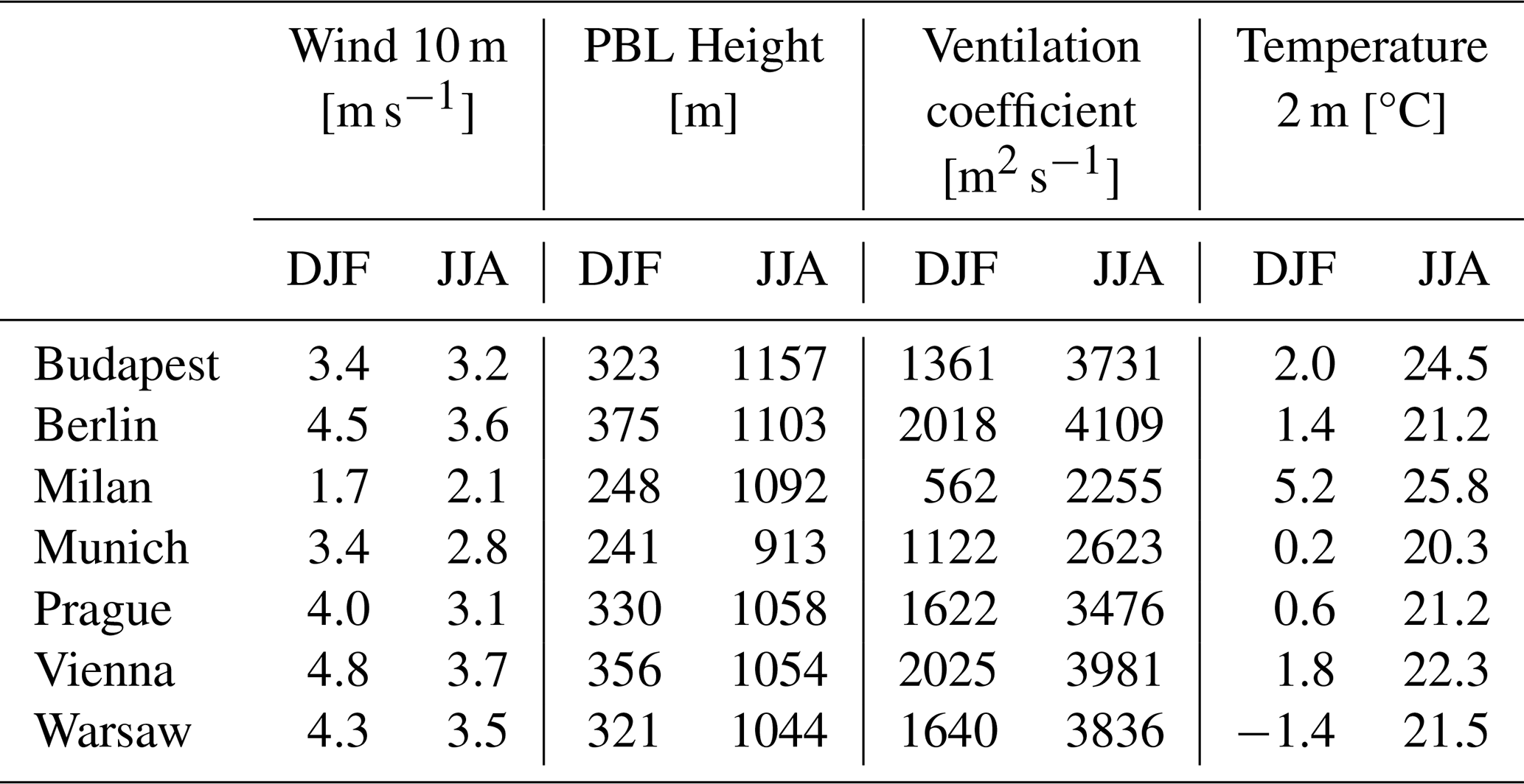
There is also a notable difference of the relative day-0 emission impact over urban areas. This is related the absolute pollution level already present over the city when the “new” day emissions are introduced. If the city exhibits good ventilation, which means high winds and elevated PBL than emissions are easily transported away making the day-0 emission impact low. To demonstrate this, we calculated the average wind-speed (at 10 m), PBL height, ventilation coefficient and 2 m temperature for winter and summer for the selected cities in Table 1. From these numbers it is clear, that Vienna and Berlin belong to the windiest cities and, indeed, they exhibit the lowest relative contribution of the actual day's emissions. On the other hand, Munich and especially Milan have the lowest ventilation coefficient in winter, resulting in slower dispersion of urban emissions resulting in high relative impact of day-0 emissions. Regarding the differences in the relative impact on the secondary components, it strongly depends the precursor composition of the urban emissions and in this regard, there are probably differences between the cities, which then causes the large inter-city differences of impact on sulfates (however, the relative impact on nitrates and ammonium are similar between the cities).

It is also clear from the results that the relative contributions from previous days' emissions are higher during winter. This is caused in general by the longer lifetime of aerosol in winter as well as longer lifetime of its precursors. This is largely determined by deposition: e.g. for SO₂ deposition in summer is much higher than in winter (Hardacre et al., 2021). Also its oxidation by the reaction with OH (hydroxyl) radical is faster in summer (Seinfeld and Pandis, 2016). For another precursor of PM, NO₂ it can be also said that its lifetime is longer in winter due to weaker solar radiation and lower atmospheric temperature, or in other words, solar radiation is stronger in summer and chemical reactions are active, which is beneficial to NO₂ removal (Wang et al., 2019), while at the same time, dry-deposition for NO₂ is also larger in summer (Aksoyoglu and Prévôt, 2018).

Regarding secondary organic aerosol, it is known that they have a shorter lifetime during summer due to increased evaporation back to the gas-phases while in winter they are more stable (Duan et al., 2020). Also, the VOC precursors to SOA more readily degrade during summer making their lifetime shorter in this season (Debevec et al., 2021). This partly explains the much higher relative contributions of previous days' emissions to SOA concentrations in winter. However, there is another reason that was seen in our simulations: during summer, biogenic VOC emissions are much stronger and they can oxidize into semi- and low-volatility substances leading to formation of biogenic SOA (Cao et al., 2022). Thus, in general, the contributions of anthropogenic emissions are lower in summer.

There is a sudden drop of values seen in the daily variability of the relative contributions for PM and basically all of its components (both primary and secondary) occurring from March to April. This is explained by the monthly temporal factors that are used to dissaggregate the annual totals. They expected a sudden decrease (to zero) of emissions from domestic combustion due to heating on 1 April. As this is the primary source of PM in urban areas, once it is switched off the contribution of anthropogenic emissions show a large drop and long range transport becomes more important (which manifests itself in the contributions from the boundary conditions - not shown in this paper).

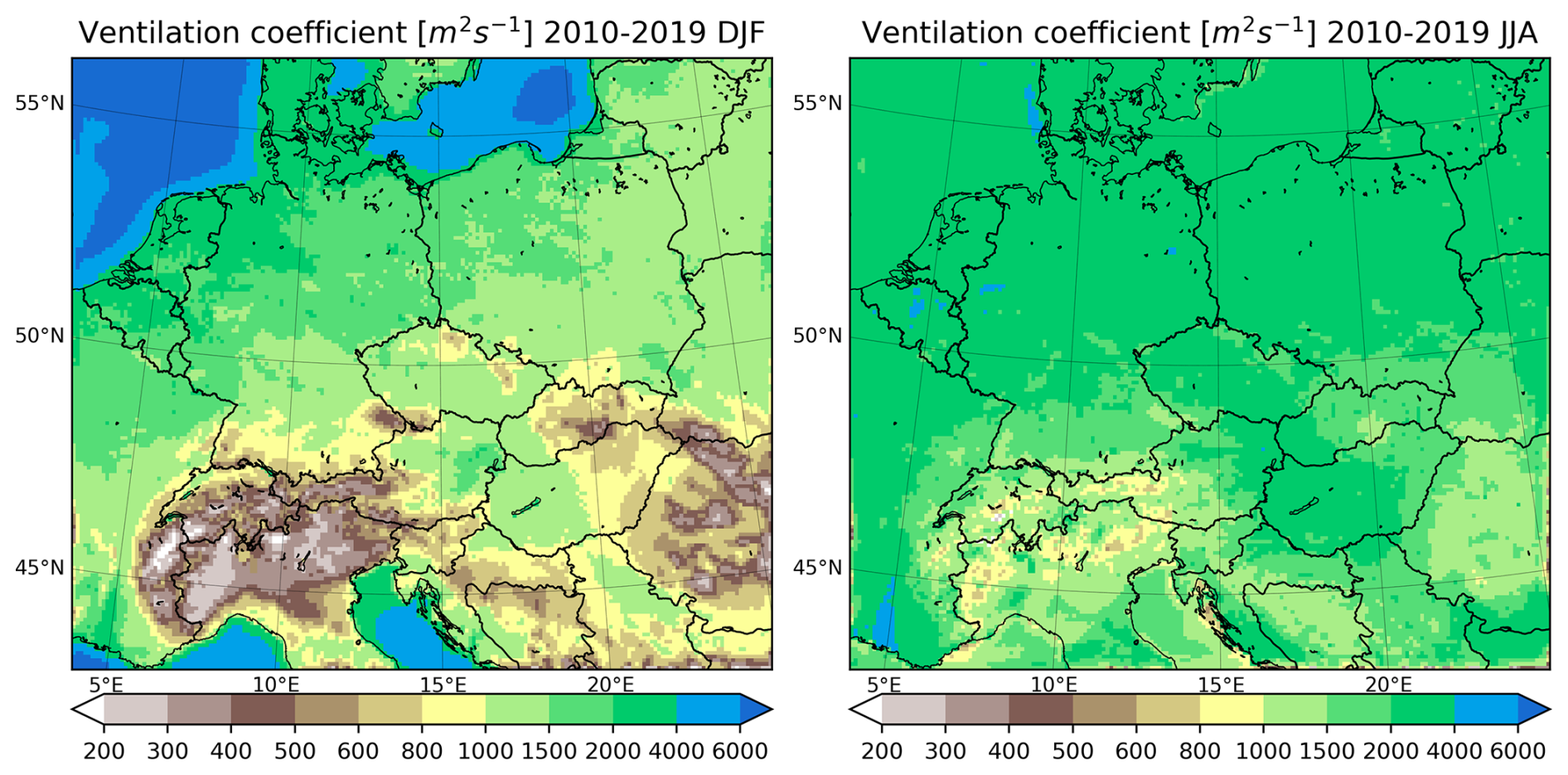
Figure 18 The 2010–2019 DJF (left) and JJA (right) average ventilation coefficient in m² s⁻¹.

The geographical distribution of the contribution from previous days' emissions shows large differences which are explained by (i) differences in emissions of primary PM and their precursors across the domain, (ii) distance from the domain boundary where the effect of the concentrations imposed to the boundaries become dominant, and finally, (iii) by the ability for emitted PM and that formed secondarily to dilute into regional scales. The highest contributions are modelled over northern Italy which is known to have one of the worst air-quality in Europe, and an important contributor to this is the reduced ventilation the Po Valley faces, as reported by EEA (2024). To support this explanation, we plotted the geographical distribution of the ventilation coefficient (C_vent; calculated as the product of the 10 m wind-speed and the boundary layer height) in Fig. 18 as DJF and JJA mean. It is clear that the lowest C_vent are modelled over northern Italy along with the Po Valley. In winter, their values are often below 300 m² s⁻¹ while in summer, the values are larger but still the lowest values are obtained for the mentioned region (around 600–800 m² s⁻¹). Another hotspot for larger contribution from past emissions is central Europe, which is again given by the combination of strong emissions and reduced ventilation during winter months. Moreover, for primary aerosol, the contributions from day-0 emissions are usually localized and align well with the emission hotspots, while this is not true for secondary aerosol, which require some time to form (Zhang et al., 2019).

Our results showed that while the average contribution of previous 1–3 d' anthropogenic emissions to PM concentration is of the order of 1 %–10 % and 0 %–0.5 % for even older emission, the variability of these is quite large. Even older emission from day-4 to day-5 can contribute for selected days by up to 10 % while one week old emissions can add up to 1 %–2 % to the daily average PM_2.5 concentrations, so considerably more than the average. The reason behind such enhanced contributions from past emissions can be both dynamical and chemical. The dynamical cause can include upward vertical mixing and transport of concentrated plumes over distant areas for several days while chemical causes mean reduced chemical decay of a particular pollutant (e.g. during winter). Moreover, under dry conditions without precipitation, wet-deposition is reduced and increases the lifetime of pollutants contributing to the above mentioned causes. For example, Wagstrom and Pandis (2009) showed that the average age of aerosol and its components increases with height in the atmosphere which confirms that transporting aerosol plumes vertically increases their lifetime and once transported back to the surface it manifests in our case as contribution from past emission. In case of secondary inorganic aerosol, the large contribution of past emissions can be caused also by slow chemical formation from primary precursors, accumulation and transport to distant areas, as shown by Ying et al. (2021) for sulfates. Also Xie et al. (2023) showed that during haze events over eastern China, stagnant weather conditions and consequent regional transport allowed particles to remain suspended in air for long times increasing the atmospheric age of polluting PM.

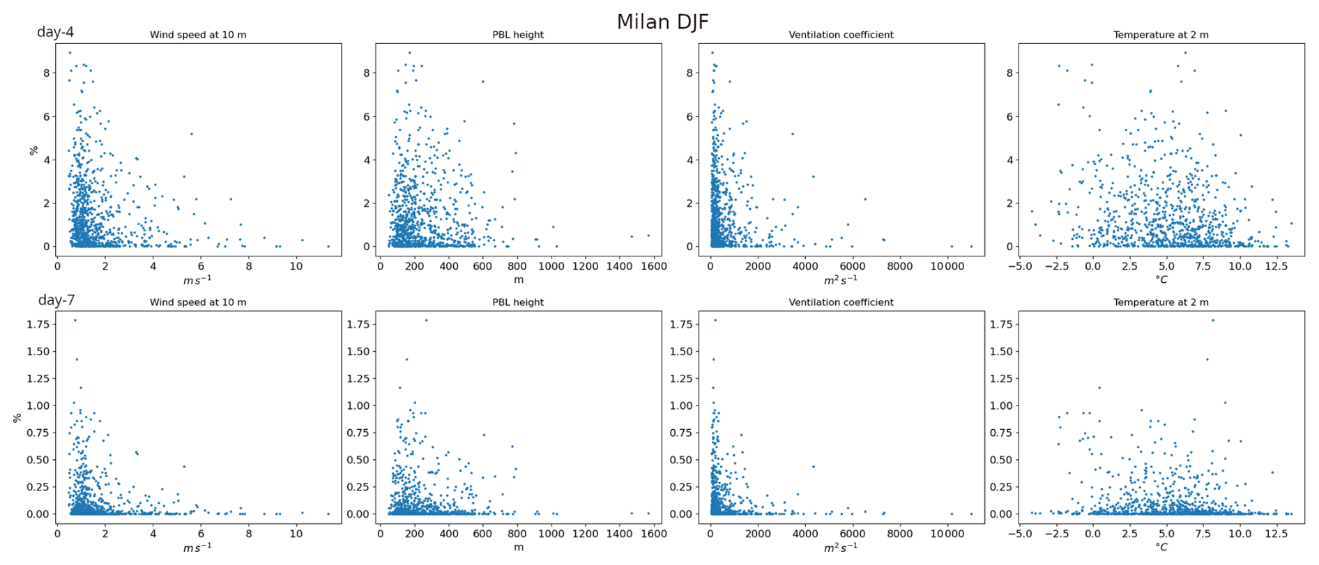
Figure 19 Scatter plots of the relative contributions of emissions from day-4 (upper row) and day-7 (lower row) to the daily mean PM_2.5 concentrations vs. the daily mean wind speed at 10 m, planetary boundary layer height, ventilation index and 2 m temperature (from left to right) for winter 2010–2019 for Milan.

Figure 20 Same as Fig. 19 but for summer.

To facilitate a better understanding of the possible meteorological (dynamical) causes for high contributions from past emissions, we depicted the scatter plot between the daily relative contributions (from day-4 and day-7) and different meteorological parameters (wind speed at 10 m, planetary boundary layer height, ventilation coefficient and 2 m air temperature) in Figs. 19 and 20 corresponding to winter and summer days while focusing on Milan. We have chosen this city as it lies in the most polluted region in the domain and is affected, as seen in our analysis by the highest contributions from previous days emissions, what is supported also by the lowest average ventilation over the corresponding region as seen in Fig. 18. However, we present also other cities and the impact of the day-7 emissions in relation to meteorological conditions in Figs. S12–S16 (in the Supplement). In winter, there is a clear indication that high relative contributions are associated with both low wind speeds and low PBL heights together acting to greatly lower the ventilation coefficient. This supports the hypothesis that stagnant winter conditions with probably strong inversions lead to accumulation of pollutants for multiple days, putting a higher role on past emissions. This is seen also for other cities for 1 week old anthropogenic emissions – very high relative contributions of such emissions are almost always associated with very low ventilation – especially in winter (as expected). As for the importance of temperature in winter, it is unequivocally seen from figures that the highest relative contributions occur for temperature in the mid-range of the total winter temperature range, close to 0 °C. Indeed, in Central Europe, the most persistent winter stagnation is typically associated with stable high-pressure episodes that create strong near-surface inversions and long-lived fog/low stratus in lowlands and this often coincides with near-freezing temperatures in the lowlands (around 0 to a few degrees below) rather than during very low or very high temperatures (Barbara et al., 2020).

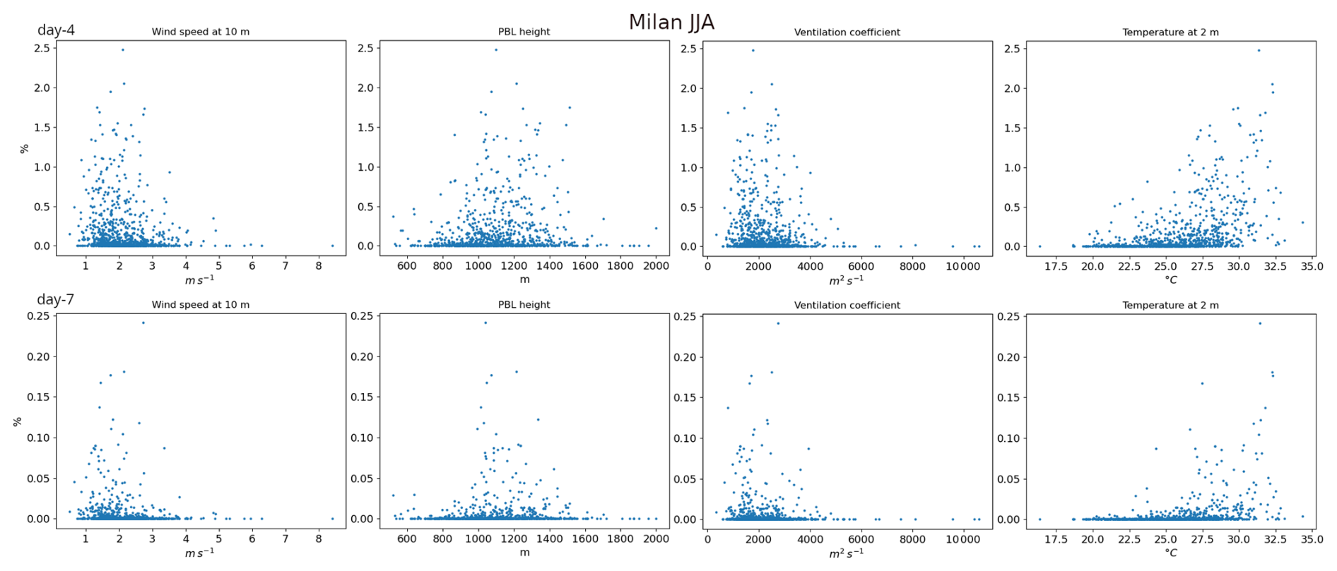
In summer, it can be seen that high relative contributions are linked to high temperatures, contrary to winter. This is evident for each analyzed city. High temperatures over this region are predominantly related to the development of anticyclonic high pressure systems with low surface winds where, due to strong subsidence, skies are clear and there is virtually no precipitation (Lhotka and Kyselý, 2024). Under these circumstances, PM can easily accumulate in the PBL (Graham et al., 2020) which still contains some thermally induced mixing due to intense heating of the surface (Zhang et al., 2013), while, at the same time, wet-deposition is missing, leading to considerable increase of the PM lifetime over the region. This is the reason why high summer contributions do not occur for very low winds or low PBL heights as these are, despite the anticyclonic stagnant conditions, still elevated due to surface heating and shallow convection.

However, we must note that the exact causes for high contributions of past emissions on individual days may deviate from the above argumentation, and it would be necessary to analyze them case by case, which would go much beyond the scope of this study; however, it is probable that the causes are rather a combination of the above mentioned circumstances related to mixing and temperature.

Our results should also be viewed in the context of the outcome of the validation. It was shown that the modelled PM as well as its gas-phase precursors (NO₂ and SO₂) were strongly underestimated. We can expect that due to this negative bias the absolute contributions of previous days emissions are underestimated, too. However, the relative contributions are probably not affected too much as these represent the ratio of the absolute contribution and total concentration.

5 Conclusions

In summary, our study reached the following conclusions:

• Winter daily PM_2.5 levels are dominated by emissions from the actual day (about 30 %–60 % contribution).

• Day-1 emissions contribute with another 20 %–30 %.

• For older emissions, the contributions decline rapidly and become negligible after 7 d.

• Both secondary inorganic and organic aerosol show similar patterns with PM_2.5 except nitrates for which the day-1 contribution is the dominant.

• Occasional episodes show substantial contributions: day-4 to day-5 emissions can contribute up to 10 %, and even week-old emissions can add 2 % in winter.

We must also point out the limitations of the study. Firstly, the comparison with measurements showed that the modelled particulate matter was strongly underestimated, caused by the combination of underestimated emissions and strong vertical mixing. As a result, we can expect that the contributions presented here are somewhat underestimated. Secondly, the annual emission totals were kept constant throughout all the simulated years, and this hindered the impact of year-to-year emission variability. Therefore, the variability presented, including extreme values of daily contributions, is predominantly caused by varying meteorological conditions rather than by abnormal emission events. Another shortcoming of the study concerns black carbon; it is an important component of the total PM and undergoes chemical aging that leads to large variations in its lifetime (Fierce et al., 2015). However, in our simulations it was considered an inert primary aerosol component, which led to very similar contributions for PEC compared to other primary aerosol. Similarly, secondary organic aerosol is also not subject to aging in the used SOA scheme, which can introduce some overestimation of the past emissions impact as it is proved that aging can decrease SOA lifetime (Rudich et al., 2007). Lastly, we calculated the contributions of emissions from different days regardless of the origin of the emissions (i.e. no spatial source apportionment was done). However, for detailed explanation whether it is the local emissions or regional ones which contribute at different age to the urban PM burdens, it is necessary to consider the geographic origin of emissions. This would be an important addition to the current research and is planned as a follow-up to this study.

Despite these caveats, our results still offer very valuable qualitative information on the importance of past emissions. The study showed that emission reduction actions taken on the day of severely deteriorated air-quality may be insufficient and should be taken a few days in advance.