Emerging low-cloud feedback and adjustment in global satellite observations

From mid-2003 to mid-2024, a global decrease in low-cloud amount enhanced the absorption of solar radiation by 0.22±0.07 W m⁻² per decade (±1σ range), accelerating the energy imbalance trend during that period (0.44 W m⁻² per decade). Through controlling factor analysis, here we show that the low-cloud trend is due to a combination of cloud feedback and adjustments to greenhouse gases and aerosols (respectively 0.09±0.02, 0.05±0.03, and 0.03±0.03 W m⁻² per decade), which jointly account for 74 % of the trend. The contribution of natural climate variability is weak but uncertain (0.01±0.08 W m⁻² per decade), owing to a poorly constrained trend in boundary-layer inversion strength. Importantly, the observed low-cloud radiative trend lies well within the range of values simulated by contemporary global climate models under conditions close to present day. Any systematic model error in the representation of present-day global energy imbalance trends is thus likely to originate in processes unrelated to low clouds.

1 Introduction

Earth's energy imbalance, the difference between absorbed shortwave and outgoing longwave radiation at the top of the atmosphere, is a key indicator of climate change. This energy imbalance is currently increasing under the combined effect of a strengthening positive greenhouse gas forcing and a weakening negative aerosol forcing (Forster et al., 2021; Loeb et al., 2021; Kramer et al., 2021; Hodnebrog et al., 2024; Forster et al., 2025). However, radiative budget trends are also influenced by processes of rapid adjustment and climate feedback, as well as natural climate variability (Raghuraman et al., 2021; Andrews et al., 2022; Raghuraman et al., 2023).

Global satellite observations reveal a rapidly increasing global energy imbalance since the early 2000s, seemingly faster than simulated by contemporary coupled global climate models (Olonscheck and Rugenstein, 2024; Mauritsen et al., 2025), but the causes of this discrepancy are unclear. Previous work has highlighted the important contribution of decreased shortwave (SW) reflection by clouds (Stephens et al., 2022; Raghuraman et al., 2023; Tselioudis et al., 2025), and particularly low clouds (Loeb et al., 2024b; Goessling et al., 2025), to the energy imbalance trends. Recent decades have seen a conjunction of factors expected to reduce low-cloud SW reflection: weakening aerosol forcing (Kramer et al., 2021; Yuan et al., 2022, 2024; Gettelman et al., 2024; Zhang et al., 2025); positive rapid adjustments to increasing greenhouse gas forcing (Gregory and Webb, 2008; Andrews and Forster, 2008; Andrews et al., 2012); and positive low-cloud feedback (Ceppi et al., 2017; Zelinka et al., 2020; Myers et al., 2021; Ceppi et al., 2024). Meanwhile, natural climate variability can cause large decadal SW low-cloud trends of either sign, particularly via the sea-surface temperature (SST) “pattern effect” (Zhou et al., 2016; Andrews et al., 2022). The relative importance of these various drivers for the recent low-cloud radiative trends remains to be quantified.

Here we apply cloud-controlling factor analysis (e.g., Scott et al., 2020; Myers et al., 2021; Ceppi and Nowack, 2021; Ceppi et al., 2024; Wilson Kemsley et al., 2024) to interpret recent low-cloud radiative trends, using state-of-the-art global satellite observations from the Clouds and the Earth’s Radiant Energy System (CERES) project, complemented by reanalysis data and Coupled Model Intercomparison Project phase 6 (CMIP6; Eyring et al., 2016) climate model simulations. We find that the low-cloud trend is driven primarily by a combination of low-cloud feedback and adjustments to aerosol and greenhouse gas (GHG) forcing. Furthermore, the observed low-cloud trend lies well within the range of global climate model simulations, suggesting that any model error in energy imbalance trends likely originates in processes unrelated to low clouds.

2 Observed radiative trends

Our analysis covers July 2003 to June 2024, where our datasets overlap (Appendix A1). For this period, Earth's global energy imbalance N as observed by CERES Energy Balanced and Filled (CERES-EBAF) increased at an average rate of 0.44 W m⁻² per decade (Fig. 1a) – a value consistent with other findings based on similar analysis periods (e.g., Hodnebrog et al., 2024; Loeb et al., 2024b; Mauritsen et al., 2025). Anomalies in SW low-cloud radiative effect (SWCRE_low, defined positive down, Appendices A1–A2), calculated from the CERES Flux-By-Cloud-Type (CERES-FBCT) product, made a large contribution amounting to half of this decadal trend, in addition to explaining a substantial portion of inter-annual variations in N (Fig. 1a; correlation coefficient r=0.82). Low clouds however only account for about a quarter of the large increase in absorbed solar radiation (0.86 W m⁻² per decade, not shown; Loeb et al., 2024b; Myhre et al., 2025), which includes additional contributions from non-low clouds, surface albedo, water vapour absorption, and shortwave forcing.

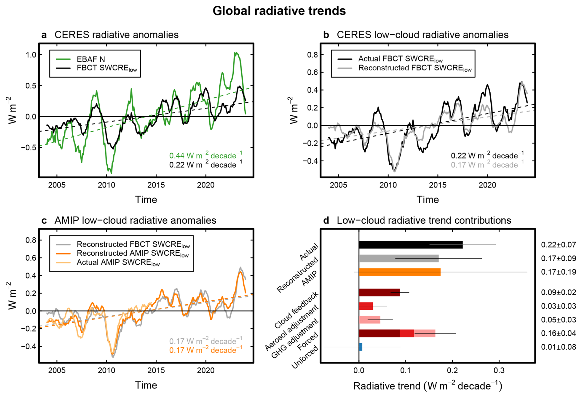
Figure 1 (a–c) Timeseries of global radiative anomalies: (a) CERES-EBAF net radiative imbalance N (green) and CERES-FBCT SWCRE_low (black); (b) CERES-FBCT SWCRE_low (black) and reconstructed timeseries (grey); (c) reconstructed CERES-FBCT SWCRE_low (grey) and CMIP6 SWCRE_low (Table A1), emulating extended amip simulations (dark orange). The actual SWCRE_low from amip simulations up to December 2014 is shown in light orange. (d) CERES-FBCT actual and reconstructed trends, amip emulated trend, and contributions to the CERES-FBCT reconstructed trend from cloud feedback, aerosol adjustment, greenhouse gas (GHG) adjustment, and unforced climate variability. Thick bars denote central estimates, while thin bars provide ±1σ ranges. Timeseries show monthly anomalies from the time mean, smoothed with a 12-month centred running mean. Coloured dashed lines represent linear fits to the corresponding timeseries, with trend values (in W m⁻² per decade, calculated before smoothing the timeseries) shown in the bottom right corner of each panel. Values are near-global averages (60° S to 60° N), scaled to the global area, except for N which uses global data.

The global SWCRE_low trend is driven by changes across the Northern Hemisphere ocean basins, Europe, the Southeast Indian Ocean, and the South Atlantic, with opposing contributions mainly in the tropical Southeast Pacific (Fig. 2a). Given that increasing surface temperature (T_sfc) generally promotes less low cloud and thus anomalously positive SWCRE_low, whereas increasing estimated inversion strength (EIS, defined in Appendix A1) has the opposite effect (Fig. A1), the spatial pattern of the SWCRE_low trend appears qualitatively consistent with the observed changes in T_sfc and EIS (Fig. 2d and e): regions of positive SWCRE_low trends coincide with regions of increasing T_sfc, and the area of negative SWCRE_low change in the tropical Southeast Pacific corresponds to an area of positive EIS change and near-zero T_sfc trend. The low-cloud radiative trends described here agree in magnitude and meridional structure with those reported in Fig. 9b of Loeb et al. (2024b) for the period July 2002 to December 2022.

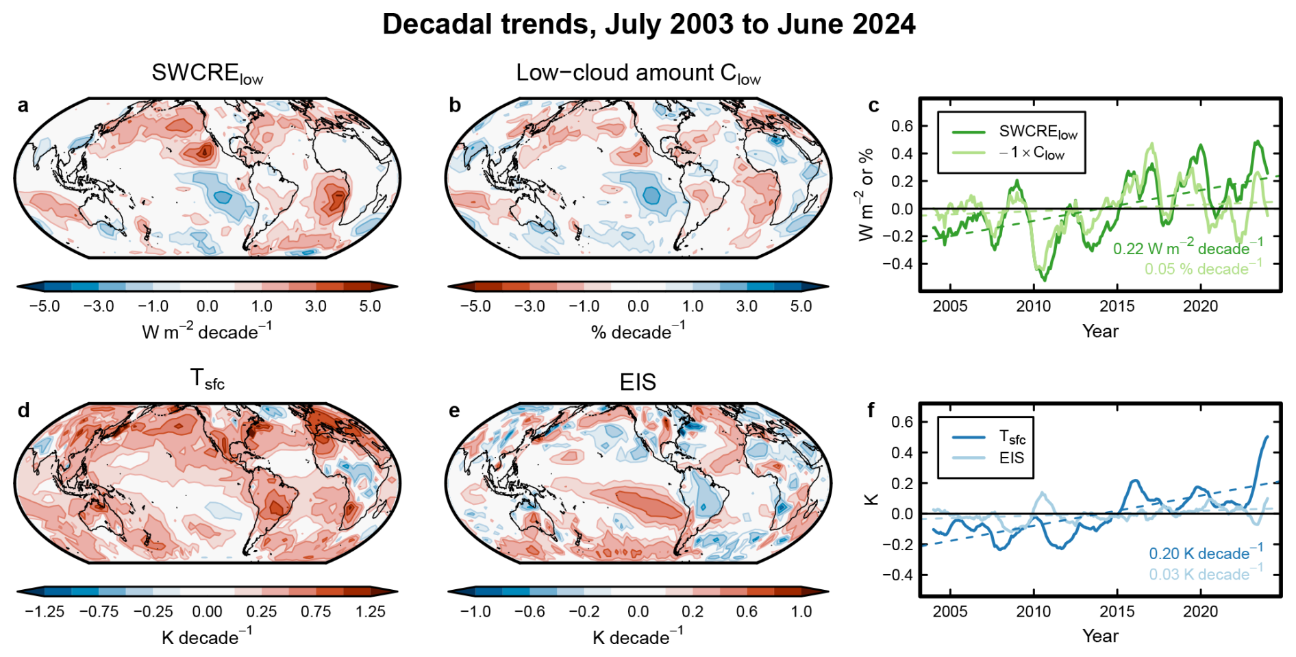
Figure 2 Observed decadal trends in (a) low-cloud radiative effect SWCRE_low, (b) low-cloud amount C_low (note the inverted colourbar), (d) surface temperature T_sfc, and (e) estimated inversion strength EIS (lower-tropospheric stability LTS over land). (c, f) Near-global timeseries of the same quantities, averaged from 60° S to 60° N and scaled to the global area. The timeseries show monthly anomalies from the time-mean, smoothed with a 12-month centred running mean. Coloured dashed lines represent linear fits to the corresponding timeseries, with trend values (in W m⁻² per decade, % per decade or K per decade, calculated before smoothing the timeseries) shown in the bottom right corner of each panel. Trend maps for other controlling factors are shown in Fig. A2.

The SWCRE_low changes also agree well with the changes in low-cloud amount, both locally and globally (Fig. 2a–c); low-cloud amount decreases globally by 0.05 % per decade during the analysis period. Consistent with this, nearly all of the SWCRE_low trend is associated with decreasing cloud amount, as opposed to decreasing optical depth (respectively 0.21 and 0.01 W m⁻² per decade; not shown), although observational uncertainties may affect this partitioning.

T_sfc increases substantially during our study period: 0.20 K per decade, or 0.44 K over 21 years. This suggests that a substantial fraction of the SWCRE_low increase may reflect an emerging low-cloud feedback in satellite observations. However, aerosol adjustment is likely to have also played a role, especially in the Northern Hemisphere, as are GHG adjustments and unforced climate variability. To distinguish between these drivers, we employ cloud-controlling factor (CCF) analysis (Appendix A3) along with global climate model estimates of the SWCRE_low GHG adjustment.

3 Drivers of the low-cloud radiative trend

The reconstruction method (Appendix A3) overall reproduces the inter-annual variability in global SWCRE_low, despite underestimating some extrema. The method also captures most of the decadal trend (0.17 W m⁻² per decade; Fig. 1b and d), even though all trends were removed during the training process, with an unexplained residual of 0.05 W m⁻² per decade. Discrepancies may arise for several reasons: inaccuracies in the CCF method, observational error in the CCFs or the cloud-radiative anomalies, stochastic cloud variability that is unaccounted for by the CCFs, errors in the climate model-based estimate of the GHG adjustment, or errors in the observed SWCRE_low trend.

The observed SWCRE_low trend is also reasonably well reproduced spatially (Fig. 3a and b), with the CCF reconstruction generally capturing the distribution of positive and negative anomalies, and a pattern correlation coefficient of 0.68. Discrepancies are found mainly in Northern Hemisphere ocean basins, as well as in Southern Hemisphere stratocumulus regions (Fig. 3c). We can further validate the method by treating each available CMIP6 historical model simulation (Appendix A1) as an observation, and showing that the reconstructed trends agree closely with the actual values (Fig. 4).

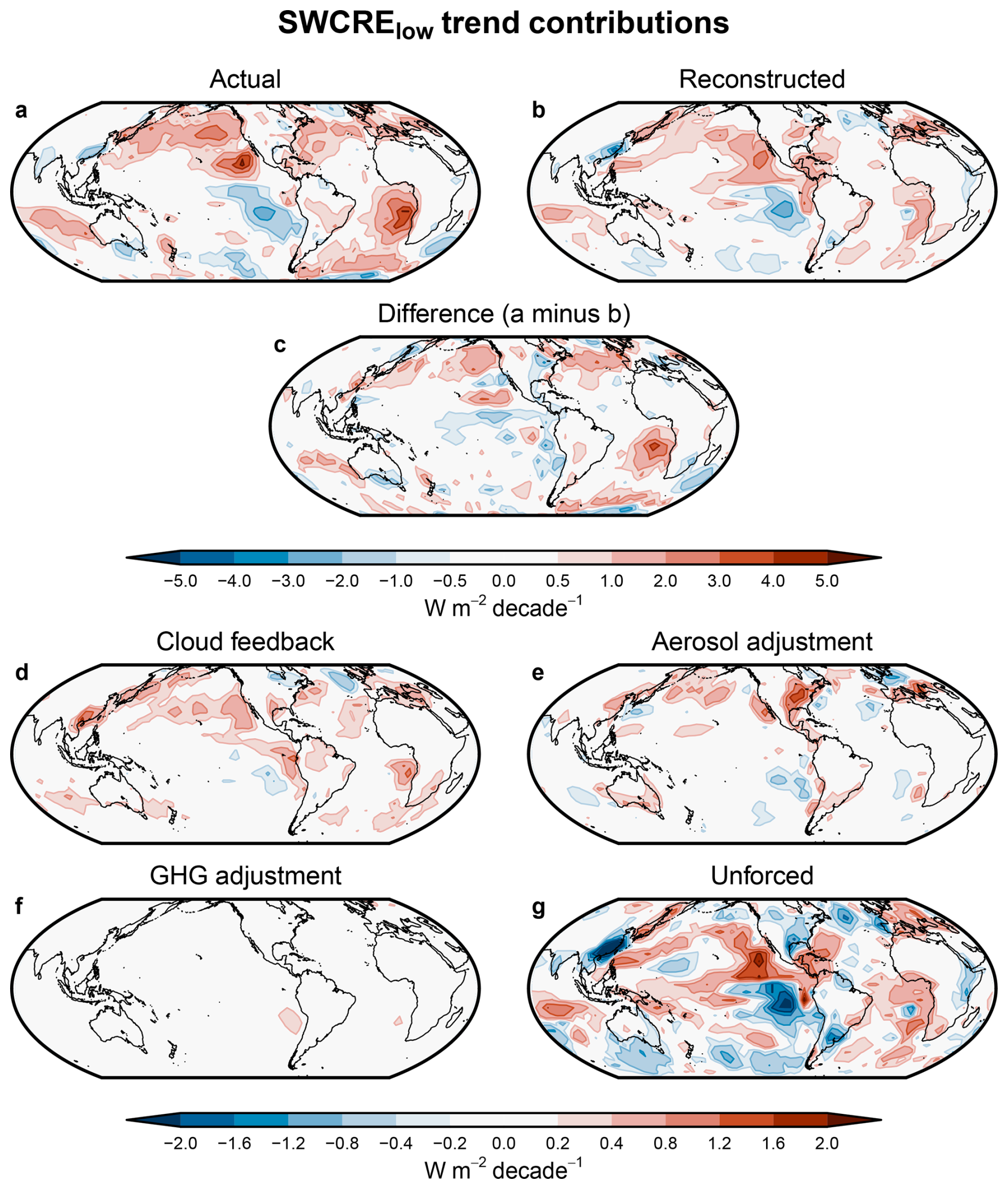
Figure 3 Maps of CERES-FBCT SWCRE_low trends, decomposed into contributions. (a) Actual SWCRE_low trend, (b) reconstructed trend (sum of panels d–g), (c) difference (a minus b), and contributions from (d) cloud feedback, (e) aerosol adjustment, (f) greenhouse gas (GHG) adjustment, and (g) unforced variability. The GHG adjustment trend contribution (f) is repeated in Fig. A3 with a finer colourbar.

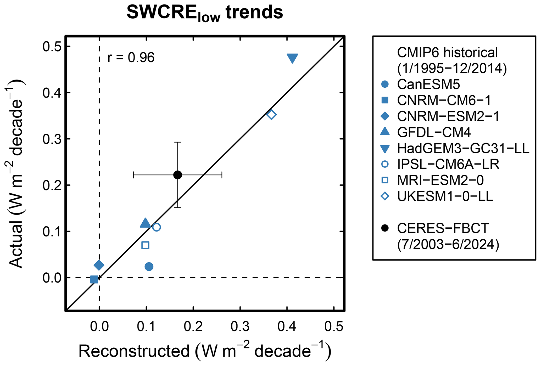
Figure 4 Comparison of actual and reconstructed trends in SWCRE_low. Blue symbols denote trends from individual CMIP6 models in the historical simulations during January 1995 to December 2014. The black circle shows CERES-FBCT values for July 2003 to June 2024, with error bars denoting ±1σ confidence intervals. The one-to-one line is shown in solid black.

We next assess the contributions of cloud feedback, adjustments to aerosols and GHG, and unforced climate variability to the observed SWCRE_low trend (Appendix A4–A5). We identify cloud feedback as the leading contribution, explaining 40 % of the observed global SWCRE_low trend (0.09±0.02 W m⁻² per decade, ±1σ range; Fig. 1d). This contribution is largest in tropical subsidence and midlatitude regions (Fig. 3d), consistent with previous observational assessments (Myers et al., 2021; Ceppi et al., 2024). Normalised by the observed warming rate, this implies a low-cloud feedback best estimate of 0.39 W m⁻² K⁻¹, consistent with the assessment of Ceppi et al. (2024).

The next largest effects are adjustments to aerosol and GHG. Aerosols contribute 0.03±0.03 W m⁻² per decade, primarily from changes in the Northern Hemisphere (Fig. 3e). This is close to the numbers of Park and Soden (2025) of 0.00 to 0.06 W m⁻² per decade depending on the aerosol dataset. GHG adjustment has a comparable impact (0.05±0.03 W m⁻² per decade), but with a much more uniform spatial pattern (Figs. 3f and A3). This positive low-cloud adjustment to GHG results from rapid lower-tropospheric warming and drying in response to GHG forcing, in addition to a reduction in radiative cooling at cloud top (Andrews et al., 2012; Kamae et al., 2015; Salvi et al., 2021; Quaas et al., 2024). Taken together, low-cloud feedback and adjustment (i.e. the forced low-cloud response) account for around 74 % of the trend (0.16±0.04 W m⁻² per decade; Fig. 1d).

Accordingly, the contribution of unforced climate variability is small at 0.01 W m⁻² per decade. This is likely coincidental and specific to the phase of climate variability for the time period considered, given the known large decadal variations in low-cloud feedback associated with time-varying SST patterns (Zhou et al., 2016; Kawaguchi and Ceppi, 2025). While small in the global mean, the unforced variability component exhibits a large uncertainty (±0.08 W m⁻² per decade) and is regionally dominant (Fig. 3g). In a global-mean sense, the magnitude and sign of the unforced variability contribution depend entirely on the choice of EIS dataset (Appendices A5–A6): across the 40 ensemble members, the unforced trend strongly correlates with the trend of the EIS contribution to SWCRE_low (r=0.86; not shown). This EIS trend uncertainty also dominates the spread in the total reconstructed SWCRE_low trend (r=0.63; Figs. A4–A5), while only contributing minimally to uncertainty in the forced component of the trend, owing to a weak forced EIS response (Fig. A2).

4 Can global climate models simulate the low-cloud trend?

Given prior findings that CMIP6 models may underestimate the recent energy imbalance trend (Olonscheck and Rugenstein, 2024; Mauritsen et al., 2025), we consider whether low clouds may account for some or all of the discrepancy. Per Eq. (A2), such a discrepancy could arise for two, not mutually exclusive reasons: (1) models are unable to simulate the CCF changes observed during the period of study (the dX term in Eq. A2); (2) models misrepresent the cloud response to the observed CCF changes (the Θ term). Additionally, models may underestimate the low-cloud adjustment to GHG forcing, but we are unable to assess that possibility here.

To evaluate model performance, we compare the observed SWCRE_low trend with that calculated from amip and historical simulations. Comparing with amip minimises differences in CCF trends between models and observations, thus highlighting the role of the cloud-radiative sensitivities (Θ). By contrast, the comparison with historical will additionally include more substantial differences in CCF trends.

The amip and historical experiments in CMIP6 end in December 2014. Hence for the comparison with amip simulations, we restrict ourselves to the overlapping period July 2003 to December 2014 (Fig. 1c, light orange). Additionally, however, we exploit CCF analysis to generate synthetic amip SWCRE_low timeseries extended up to June 2024, by convolving each model's own CCF sensitivities (calculated from independent historical simulations) with the observed CCF anomalies (Fig. 1c, dark orange). In either case, the multi-model amip results agree well with CERES observations, in terms of both year-to-year fluctuations and the long-term trend (Fig. 1c). The reconstructed amip trend is nearly identical to that reconstructed from observed sensitivities (0.17 W m⁻² per decade in either case), although this is highly model-dependent (±1σ inter-model range −0.01 to +0.36 W m⁻² per decade). Overall, the comparison suggests that the observed SWCRE_low trend lies well within the range of what contemporary climate models would simulate if extended amip simulations were available.

Now turning to the historical experiment, since the CCF changes are not constrained by observed sea-surface temperatures, a perfect time overlap is not necessary and we therefore use the most recent 20-year period, January 1995 to December 2014, for our comparison. Here again, the CERES SWCRE_low trend lies fully within the range of model-simulated trends, if towards the upper end of the distribution (Fig. 4). The two models simulating stronger positive trends – two versions of the UK Met Office model, HadGEM3-GC31-LL and UKESM1-0-LL – are also at the upper end of the CMIP6 range in terms of their low-cloud feedback (Ceppi et al., 2024, their Table S2).

A limitation of our analysis is that the results in Figs. 1c and 4 are based on a limited set of CMIP6 models, including several high-sensitivity models (Table A1), meaning we cannot reliably assess any systematic model bias. Furthermore, the trends in Fig. 4 are likely strongly influenced by the phase of natural climate variability in individual realisations, and hence a quantitative comparison between models and observations would require the use of large ensembles, as in Olonscheck and Rugenstein (2024). Besides, forced CCF trends during 1995–2014 likely differ slightly from those acting in the observational period 2003–2024. These limitations notwithstanding, the results indicate that contemporary global climate models are able to simulate SWCRE_low trends similar to those observed, whether or not they are constrained to follow the specific phase of observed climate variability.

5 Conclusions

Earth's energy imbalance grew by 0.44 W m⁻² per decade between July 2003 and June 2024. Over this 21-year period, this amounts to an increase of 0.92 W m⁻², as large as the mean imbalance itself (Mauritsen et al., 2025) and potentially in excess of the rate simulated by contemporary global climate models (Olonscheck and Rugenstein, 2024). Using cloud-controlling factor (CCF) analysis, combined with climate model-derived estimates of rapid adjustments to greenhouse gas (GHG) forcing, we show that shortwave (SW) radiative changes by low clouds substantially contribute to this energy imbalance increase, at 0.22 W m⁻² per decade. The low-cloud trends, in turn, are driven by a combination of low-cloud feedback, sulphate aerosol adjustment, and GHG adjustment, which jointly account for around 74 % of the trend. This leaves only a minor role for natural climate variability, although our estimate is subject to a substantial uncertainty related to trends in 700 hPa temperature and thus EIS (Appendix A6). Our assessment of the forced and natural variability components additionally depends on the assumption that climate models realistically represent forced CCF trends.

A comparison with CMIP6 amip and historical global climate model simulations reveals that, for either experiment, observed SW low-cloud trends lie well within the range of simulated trends. In particular, emulated amip trends agree well with CERES observations in a multi-model mean sense. Based on this comparison, the observed substantial low-cloud radiative trend cannot be interpreted as evidence of an unexpectedly strong low-cloud feedback that climate models are systematically missing. A caveat is that the comparison is based on a limited set of climate models (Table A1), and furthermore the result will depend on the fidelity of aerosol emission datasets used to force the models (Hodnebrog et al., 2024; Park and Soden, 2025).

In light of our findings, it remains unclear why state-of-the-art climate models appear to generally underestimate recent trends in global energy imbalance (Schmidt et al., 2023; Olonscheck and Rugenstein, 2024; Hodnebrog et al., 2024; Mauritsen et al., 2025). We propose that further research should quantify and constrain the contributions of processes unrelated to low clouds to the observed and modelled energy imbalance trends, including their decomposition into forcing and radiative response (Raghuraman et al., 2021).

Appendix A: Data and methods

A1 Data

We use monthly gridded global satellite observations of cloud amount and top-of-atmosphere radiative fluxes from the CERES Flux-By-Cloud-Type (CERES-FBCT) product (Sun et al., 2022). We combine Edition 4A fluxes from Terra and Aqua up to April 2022 with Edition 1B fluxes from NOAA-20 for the remainder of the analysis period, taking care to minimise discontinuities between the two products (Appendix A2). While the CERES-FBCT record starts in July 2002, the Copernicus Atmosphere Monitoring Service (CAMS) aerosol reanalysis (described below) is only available from January 2003. We choose to analyse the last 21 years of available data, July 2003 to June 2024.

Since CERES-FBCT fluxes are provided as a function of cloud-top pressure, we can isolate the contribution of low clouds (cloud-top pressure greater than 680 hPa) to radiation budget changes (Appendix A2). Note that from CERES-FBCT, we can calculate cloud-radiative effect rather than true cloud-induced radiative anomalies, and hence the fluxes are subject to cloud masking effects (Soden et al., 2004); these are however expected to be much smaller for SW than longwave (LW) fluxes, particularly since we exclude regions poleward of 60° where surface albedo changes are largest (Raghuraman et al., 2023). This, combined with the fact the LW effects of low clouds are small, motivates our focus on SW cloud-radiative effect (CRE) anomalies, hereafter denoted SWCRE_low (defined positive downward). We do not analyse LWCRE data here, since their trend is dominated by cloud masking effects (Raghuraman et al., 2023), and furthermore low-cloud properties only have a modest impact on top-of-atmosphere LW fluxes.

To provide context for the low-cloud trends, we additionally use estimates of the net top-of-atmosphere radiative budget (hereafter N) from CERES Energy Balanced and Filled (CERES-EBAF) observations, Edition 4.2 (Loeb et al., 2018). When summed over all cloud types, the cloud-radiative changes diagnosed from CERES-FBCT provide a close match to those obtained from CERES-EBAF, at least over the period covered by the Terra and Aqua satellites (Loeb et al., 2024b), making CERES-FBCT ideally suited for quantifying the contributions of different cloud types to changes in Earth's energy imbalance.

We consider six meteorological drivers of cloud property changes, hereafter cloud-controlling factors (CCFs): surface temperature, T_sfc; estimated inversion strength, EIS (Wood and Bretherton, 2006); 700 hPa relative humidity, RH₇₀₀; 700 hPa pressure velocity, ω₇₀₀; horizontal air-temperature advection across the SST gradient, SSTadv; and near-surface wind speed, WS. Note that over land, instead of EIS we use the simpler metric of lower-tropospheric stability (Klein and Hartmann, 1993), as the EIS metric involves assumptions that would only hold over the ocean surface. The physical relevance of the six meteorological controlling factors is reviewed in Table 1 of Klein et al. (2017). In addition to these meteorological CCFs, we include a seventh CCF representing aerosol effects. Following previous literature (Wall et al., 2022; Park and Soden, 2025), this is either the base-10 logarithm of sulphate aerosol optical depth at 550 nm, hereafter log(AOD); or the logarithm of lower-tropospheric sulphate mass concentration, hereafter log(s).

Controlling factor data are taken from the the European Centre for Medium-Range Weather Forecasts (ECMWF) reanalysis, version 5 (ERA5; Hersbach et al., 2020) and the Modern-Era Retrospective analysis for Research and Applications, version 2 (MERRA2; Gelaro et al., 2017). Because EIS trends are sufficiently uncertain as to impact the results (Appendix A6, Figs. A4 and A5; see also Myers et al., 2023), we include an additional three independent estimates: the JRA3Q reanalysis (Kosaka et al., 2024), the Atmospheric Infrared Sounder (AIRS) satellite product, version 7 (Aumann et al., 2003), and the Community Long-term Infrared Microwave Combined Atmospheric Product System (CLIMCAPS) satellite product, version 2 (Smith and Barnet, 2023). Note that CLIMCAPS uses AIRS observations, but combined with additional instruments and processed with a different algorithm. Since EIS trend discrepancies primarily depend on the evolution of 700 hPa temperature (T₇₀₀; not shown), we combine AIRS and CLIMCAPS T₇₀₀ with ERA5 surface temperature and sea-level pressure to calculate EIS, while in other cases the values are taken from the corresponding reanalysis product. For log(AOD) and log(s), we consider two reanalysis products: CAMS, and MERRA2. log(s) is taken at 925 hPa for CAMS, and 910 hPa for MERRA2. The dependence of CCF trends on the choice of dataset is illustrated in Figs. A4 and A5 and discussed in Appendix A6.

We perform a similar analysis with CMIP6 global climate model simulations. SWCRE_low is calculated using International Satellite Cloud Climatology Project (ISCCP; Rossow and Schiffer, 1999) satellite simulator output (Bodas-Salcedo et al., 2011) convolved with cloud-radiative kernels (Zelinka et al., 2012), accounting for effects of obscuration by non-low clouds (Zelinka et al., 2025). This calculation isolates the radiative impact of cloud properties from other, non-cloud factors, and strictly speaking provides cloud-induced radiative anomalies rather than CRE. We define low-cloud radiative anomalies using the lowest three ISCCP simulator levels (instead of two for CERES-FBCT) owing to a known ISCCP bias (Myers et al., 2021; Ceppi et al., 2024).

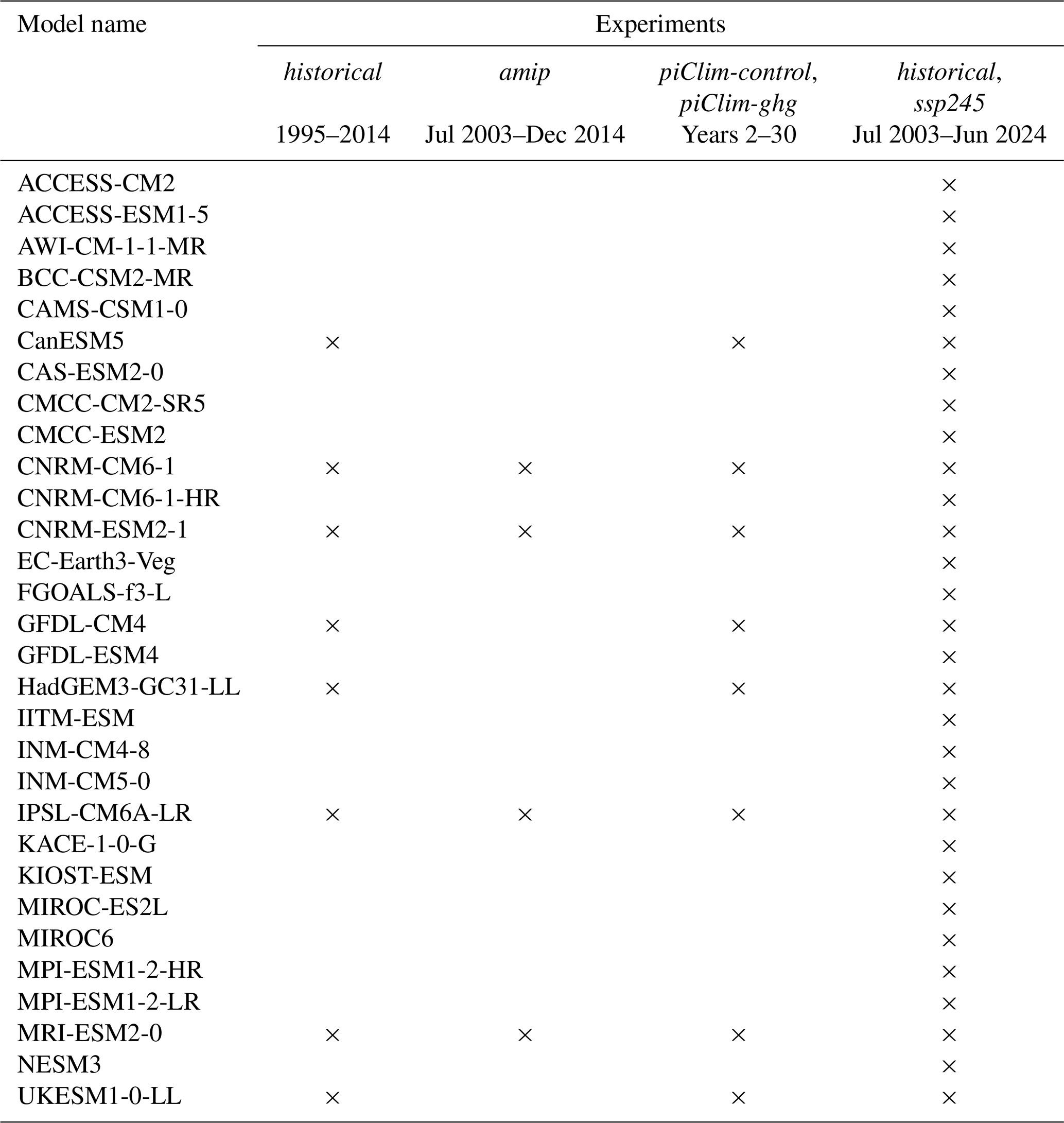
CMIP6 CCF sensitivities are calculated from the final 20 years of the CMIP6 historical experiment, January 1995 to December 2014. We additionally use data from the amip, ssp245, piClim-control, and piClim-ghg experiments; the models, variables and time periods used for each experiment are summarised in Table A1.

All observed and simulated fields are in monthly resolution, and are remapped to a common 5°×5° grid in longitude and latitude prior to statistical analysis.

Table A1 List of CMIP6 models used in the analysis, with the corresponding experiments and time periods used. A cross (×) denotes available data.

A2 Calculation of CERES-FBCT low-cloud radiative effect

CERES-FBCT data consist of clear-sky radiative flux R_clr, cloudy-sky radiative flux R_cld, and cloud amount f, with the latter two partitioned according to seven cloud-top pressure (p) bins and six cloud optical depth (τ) bins. All-sky top-of-atmosphere flux in a gridbox, R, is defined as

$$\begin{array}{}\text{(A1)}& \begin{array}{rl}R& =\left(\mathrm{1}-f_{\mathrm{tot}}\right)R_{\mathrm{clr}}+\sum _p\sum _{\mathit{\tau }}f(p,\mathit{\tau })R_{\mathrm{cld}}(p,\mathit{\tau })\\ & =R_{\mathrm{clr}}+\sum _p\sum _{\mathit{\tau }}f(p,\mathit{\tau })\left[R_{\mathrm{cld}}(p,\mathit{\tau })-R_{\mathrm{clr}}\right],\end{array}\end{array}$$

where $f_{\mathrm{tot}}=\sum _p\sum _{\mathit{\tau }}f(p,\mathit{\tau })$ is total cloud amount. The product $f(p,\mathit{\tau })R_{\mathrm{cld}}(p,\mathit{\tau })$ thus represents the contribution to all-sky flux from clouds in a given bin. Following previous literature, we categorise clouds in the lowest two pressure bins (p>680 hPa) as low clouds. We use only the SW component of the clear- and cloudy-sky fluxes, denoted R_SWclr and R_SWcld.

For the passive satellite retrievals used here, month-to-month variations in low-cloud amount L could arise simply because of changes in the amount of upper-level clouds U obscuring lower-level clouds. To isolate the contribution of low clouds, we make an assumption of random overlap between low and upper-level clouds. For each (p,τ) bin, we thus define non-obscured low-cloud amount L_n as

$$L_{\mathrm{n}}(p,\mathit{\tau })={\displaystyle \frac{L(p,\mathit{\tau })}{\mathrm{1}-U}},$$

where 1−U is the upper-level clear-sky fraction. Note that U is vertically integrated over upper-level (non-low) pressure bins, and is therefore not a function of p.

To obtain low-cloud radiative fluxes, we define the difference $K_{\mathrm{SW}}(p,\mathit{\tau })=R_{\mathrm{SWcld}}(p,\mathit{\tau })-R_{\mathrm{SWclr}}$, which quantifies how top-of-atmosphere radiation changes in the presence versus absence of clouds for each month and (p,τ) bin (cf. Eq. A1), similar to a cloud-radiative kernel (Zelinka et al., 2012). We can then calculate the low-cloud contribution to top-of-atmosphere SWCRE, SWCRE_low, by convolving K_SW with non-obscured low-cloud amount L_n, and summing over the lowest two p bins and all six τ bins:

$${\mathrm{SWCRE}}_{\mathrm{low}}=(\mathrm{1}-\stackrel{\mathrm{‾}}{U})\sum _{p=\mathrm{1}}^{\mathrm{2}}\sum _{\mathit{\tau }=\mathrm{1}}^{\mathrm{6}}{K}_{\mathrm{SW}}{L}_{\mathrm{n}},$$

where $\stackrel{\mathrm{‾}}{U}$ is the climatological value of U. Note that this calculation uses absolute low-cloud amount values (rather than anomalies) and thus provides absolute radiative flux contributions (the contribution of low clouds to SW cloud-radiative effect). Note also that accounting for obscuration by upper-level clouds, as done here, has little impact on the results, decreasing the SWCRE_low trend by just 0.007 W m⁻² per decade (not shown).

As a final step before calculating the CCF sensitivities, we normalise SWCRE_low to annual-mean insolation conditions, as seasonal changes in insolation affect SWCRE_low in the absence of any physical cloud changes, thus constituting a confounding factor. We thus define ${\mathrm{SWCRE}}_{\mathrm{low}}^{\prime }={\mathrm{SWCRE}}_{\mathrm{low}}\times \stackrel{\mathrm{‾}}{S}/S$, where S is top-of-atmosphere downward SW and the overbar denotes the annual-mean climatology. We then use SWCRE${}_{\mathrm{low}}^{\prime }$ in the ridge regression (Appendix A3) to calculate the CCF sensitivities.

CERES-FBCT fluxes come from two products covering different time periods. The Edition 4A product is based on retrievals from the Terra and Aqua satellites during September 2002 to February 2023; the Edition 1B product instead uses retrievals from NOAA-20 and covers the period May 2018 to July 2024. Loeb et al. (2024a) have documented a discontinuity in CERES-EBAF radiative fluxes between the two satellites, and described a method exploiting the time overlap between the two products to adjust the NOAA-20 fluxes and anchor them to the Terra–Aqua values. Here, we follow the same procedure to merge the two CERES-FBCT products. The procedure is applied to SWCRE_low, meaning that we first separately calculate SWCRE_low for each of the two products, then apply the method below to combine the SWCRE_low values.

We use the four-year overlap period May 2018 to April 2022 – excluding May 2022 to February 2023, to minimise the impact of drift in the Terra–Aqua record (Loeb et al., 2024a). For this period we calculate monthly SWCRE_low climatologies at each gridpoint for both products, compute the climatology difference for each gridpoint and calendar month, and subtract this difference from the NOAA-20 values over the entire record. This yields a modified CERES-FBCT NOAA-20 product whose SWCRE_low climatology during the overlap period is identical to that of the Terra–Aqua product. Finally, we concatenate the Terra–Aqua data up to April 2022 with the modified NOAA-20 data from May 2022 to July 2024, to produce a single record from September 2002 to July 2024.

A3 Cloud-controlling factor analysis framework

The CCF analysis approach follows Ceppi et al. (2024), with the addition of an aerosol CCF following Wall et al. (2022). Briefly, the low-cloud SWCRE anomalies at each location r, dSWCRE_low(r), are modelled as

$$\begin{array}{}\text{(A2)}& \begin{array}{rl}{\mathrm{dSWCRE}}_{\mathrm{low}}\left(r\right)& \approx \sum _{i=\mathrm{1}}^{\mathrm{7}}{\displaystyle \frac{\partial {\mathrm{SWCRE}}_{\mathrm{low}}\left(r\right)}{\partial {\mathit{X}}_i\left(r\right)}}\cdot \mathrm{d}{\mathit{X}}_i\left(r\right)\\ & =\sum _{i=\mathrm{1}}^{\mathrm{7}}{\mathbf{\Theta }}_i\left(r\right)\cdot \mathrm{d}{\mathit{X}}_i\left(r\right),\end{array}\end{array}$$

where X_i represents one of seven CCFs, and Θ_i denotes the sensitivity of SWCRE_low to each CCF X_i. To model SWCRE_low at each point r, we use CCF information from a 5×5 regional domain (in gridbox units) centred around r; hence X_i and Θ_i are spatial vectors, denoted by bold typeface in Eq. (A2). The sensitivities Θ_i are calculated via ridge regression, where all variables (including SWCRE_low) have been deseasonalised, and the CCF predictors have been standardised. Different from Ceppi et al. (2024), we additionally linearly detrend all variables prior to calculating the regressions; this ensures that the trend we are attempting to explain is not part of the training data. Following prior studies, we ignore any seasonality or mean-state dependence of the sensitivities Θ_i, which have been shown to have strong out-of-sample predictive skill in both models and observations (Ceppi et al., 2024). Note also that we do not account for potential effects of incomplete activation of aerosol droplets, which would likely yield a smaller estimate of the aerosol effect (Park et al., 2025).

We train on the 20-year period January 2003 to December 2022, such that the large positive SWCRE_low anomaly in 2023 is predicted entirely out-of-sample (Fig. 1b). The resulting cloud-radiative sensitivities (Fig. A1) are in agreement with previous findings (Scott et al., 2020; Myers et al., 2021; Ceppi et al., 2024). Previous studies have documented the ability of the CCF analysis method to capture cloud-radiative anomalies, whether driven thermodynamically (e.g., the response to global warming; Myers et al., 2021; Ceppi et al., 2024) or dynamically (e.g., storm track shifts; Zelinka et al., 2018; Grise and Kelleher, 2021).

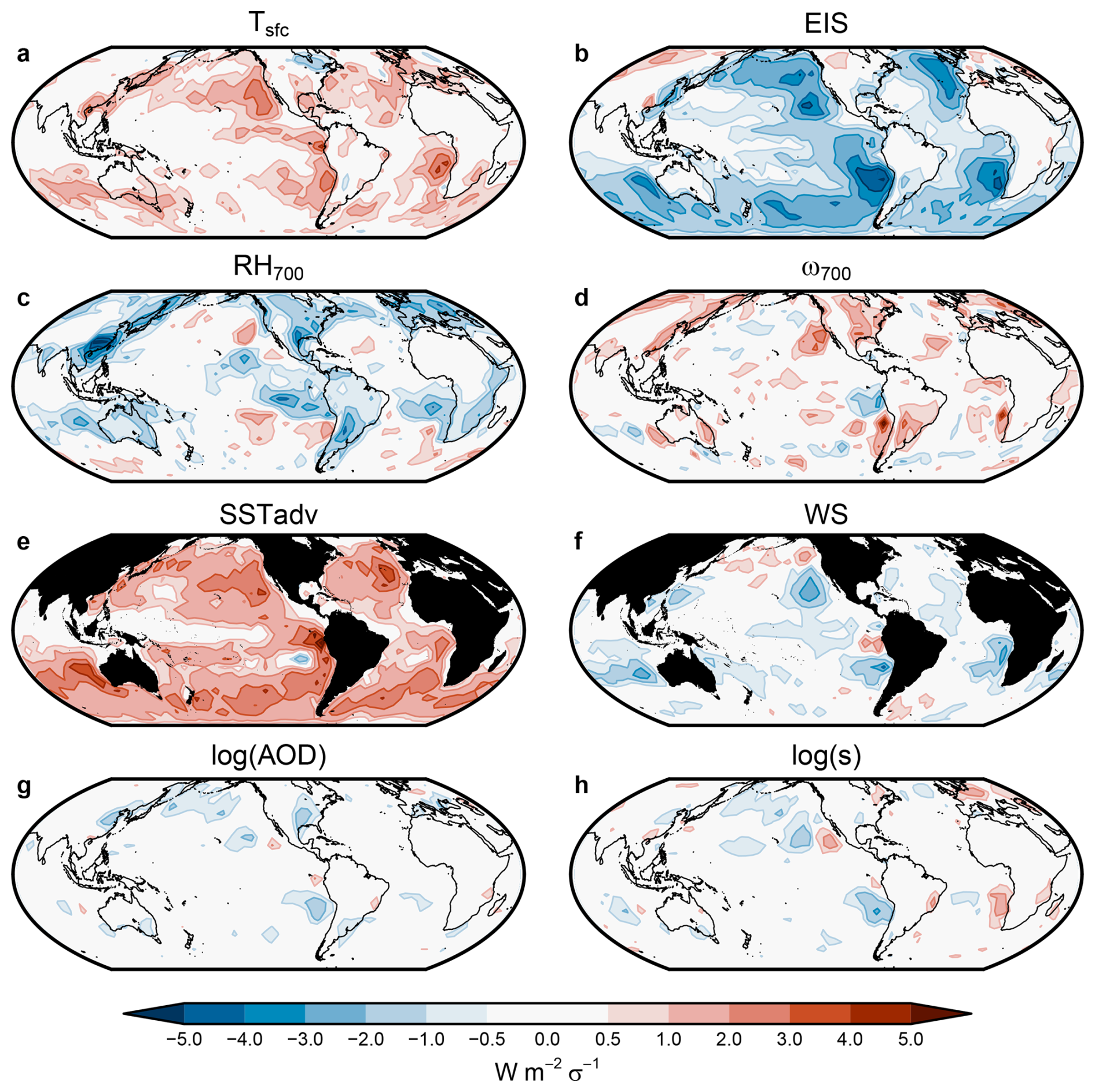
Figure A1 Maps of the cloud-radiative sensitivities to each controlling factor, representing the average sensitivity across all ensemble members (Appendix A5). While the sensitivity maps are four-dimensional (one regional map per target gridbox), for visualisation purposes we sum over regional domains to yield two-dimensional maps.

A4 Trend decomposition method

We decompose the reconstructed, observed SWCRE_low trend, $\frac{{\mathrm{dSWCRE}}_{\mathrm{low}}}{\mathrm{d}t}{|}_{\mathrm{rec}}$, into a forced component ($\frac{{\mathrm{dSWCRE}}_{\mathrm{low}}}{\mathrm{d}t}{|}_{\mathrm{for}}$) and a contribution due to unforced climate variability ($\frac{{\mathrm{dSWCRE}}_{\mathrm{low}}}{\mathrm{d}t}{|}_{\mathrm{unf}}$). We assume that the forced component is itself driven by a combination of cloud feedback ($\frac{{\mathrm{dSWCRE}}_{\mathrm{low}}}{\mathrm{d}t}{|}_{\mathrm{fdbk}}$) and adjustments to sulphate aerosol ($\frac{{\mathrm{dSWCRE}}_{\mathrm{low}}}{\mathrm{d}t}{|}_{\mathrm{aer}}$) and GHG ($\frac{{\mathrm{dSWCRE}}_{\mathrm{low}}}{\mathrm{d}t}{|}_{\mathrm{GHG}}$):

$$\begin{array}{}\text{(A3)}& \begin{array}{rl}{\displaystyle \frac{{\mathrm{dSWCRE}}_{\mathrm{low}}}{\mathrm{d}t}}{|}_{\mathrm{rec}}& ={\displaystyle \frac{{\mathrm{dSWCRE}}_{\mathrm{low}}}{\mathrm{d}t}}{|}_{\mathrm{for}}+{\displaystyle \frac{{\mathrm{dSWCRE}}_{\mathrm{low}}}{\mathrm{d}t}}{|}_{\mathrm{unf}}\\ & ={\displaystyle \frac{{\mathrm{dSWCRE}}_{\mathrm{low}}}{\mathrm{d}t}}{|}_{\mathrm{fdbk}}+{\displaystyle \frac{{\mathrm{dSWCRE}}_{\mathrm{low}}}{\mathrm{d}t}}{|}_{\mathrm{aer}}\\ & +{\displaystyle \frac{{\mathrm{dSWCRE}}_{\mathrm{low}}}{\mathrm{d}t}}{|}_{\mathrm{GHG}}+{\displaystyle \frac{{\mathrm{dSWCRE}}_{\mathrm{low}}}{\mathrm{d}t}}{|}_{\mathrm{unf}}.\end{array}\end{array}$$

The above contributions are calculated from CCF analysis, except for GHG adjustment (described below). We first describe how the CCF trends are decomposed, before explaining the calculation of the radiative trend components.

A4.1 CCF trend decomposition

We first decompose the observed trends of the six meteorological (i.e.ñon-aerosol) CCFs into forced and unforced components, where the forced component is in turn driven by a combination of SST changes and adjustments to GHG forcing:

$$\begin{array}{}\text{(A4)}& \begin{array}{rl}{\displaystyle \frac{\mathrm{d}X}{\mathrm{d}t}}& ={\displaystyle \frac{\mathrm{d}X}{\mathrm{d}t}}{|}_{\mathrm{for}}+{\displaystyle \frac{\mathrm{d}X}{\mathrm{d}t}}{|}_{\mathrm{unf}}\\ & ={\displaystyle \frac{\mathrm{d}X}{\mathrm{d}t}}{|}_{\mathrm{SST}}+{\displaystyle \frac{\mathrm{d}X}{\mathrm{d}t}}{|}_{\mathrm{GHG}}+{\displaystyle \frac{\mathrm{d}X}{\mathrm{d}t}}{|}_{\mathrm{unf}},\end{array}\end{array}$$

where X refers to a meteorological CCF. Different from the meteorological CCF trends, we treat the observed aerosol CCF trend as entirely forced: $\frac{\mathrm{d}\log \left(\mathrm{AOD}\right)}{\mathrm{d}t}=\frac{\mathrm{d}\log \left(\mathrm{AOD}\right)}{\mathrm{d}t}{|}_{\mathrm{for}}$, $\frac{\mathrm{d}\log \left(\mathrm{s}\right)}{\mathrm{d}t}=\frac{\mathrm{d}\log \left(\mathrm{s}\right)}{\mathrm{d}t}{|}_{\mathrm{for}}$.

We use climate model simulations to calculate the terms on the right-hand side of Eq. (A4), as follows:

• First, we estimate the forced meteorological CCF trend component, $\frac{\mathrm{d}X}{\mathrm{d}t}{|}_{\mathrm{for}}$, as the CMIP6-mean trend in the combined historical and ssp245 experiments from July 2003 to June 2024, based on output from 30 models (Table A1).

• Next, for the GHG adjustment-induced trend, $\frac{\mathrm{d}X}{\mathrm{d}t}{|}_{\mathrm{GHG}}$, we use the CMIP6-mean CCF response from experiments piClim-ghg and piClim-control (Table A1). This represents the CCF adjustment as of year 2014, relative to the pre-industrial control. To assess the corresponding trend contribution, we scale the year 2014 CCF anomalies according to the trend of the ratio of greenhouse gas forcing relative to year 2014, using radiative forcing values from Forster et al. (2025).

• The SST-mediated CCF trend is then obtained as $\frac{\mathrm{d}X}{\mathrm{d}t}{|}_{\mathrm{SST}}=\frac{\mathrm{d}X}{\mathrm{d}t}{|}_{\mathrm{for}}-\frac{\mathrm{d}X}{\mathrm{d}t}{|}_{\mathrm{GHG}}$.

• Finally, the unforced CCF trend is calculated as $\frac{\mathrm{d}X}{\mathrm{d}t}{|}_{\mathrm{unf}}=\frac{\mathrm{d}X}{\mathrm{d}t}-\frac{\mathrm{d}X}{\mathrm{d}t}{|}_{\mathrm{for}}$, i.e. the residual observed trend.

The resulting forced and unforced CCF trends are shown in Fig. A2. Although different sets of CMIP6 models are used for the calculation of $\frac{\mathrm{d}X}{\mathrm{d}t}{|}_{\mathrm{for}}$ and $\frac{\mathrm{d}X}{\mathrm{d}t}{|}_{\mathrm{GHG}}$ (Table A1), we obtain a very similar decomposition of the CCF trends if we instead use a smaller common set of eight models to calculate both $\frac{\mathrm{d}X}{\mathrm{d}t}{|}_{\mathrm{for}}$ and $\frac{\mathrm{d}X}{\mathrm{d}t}{|}_{\mathrm{GHG}}$ (not shown).

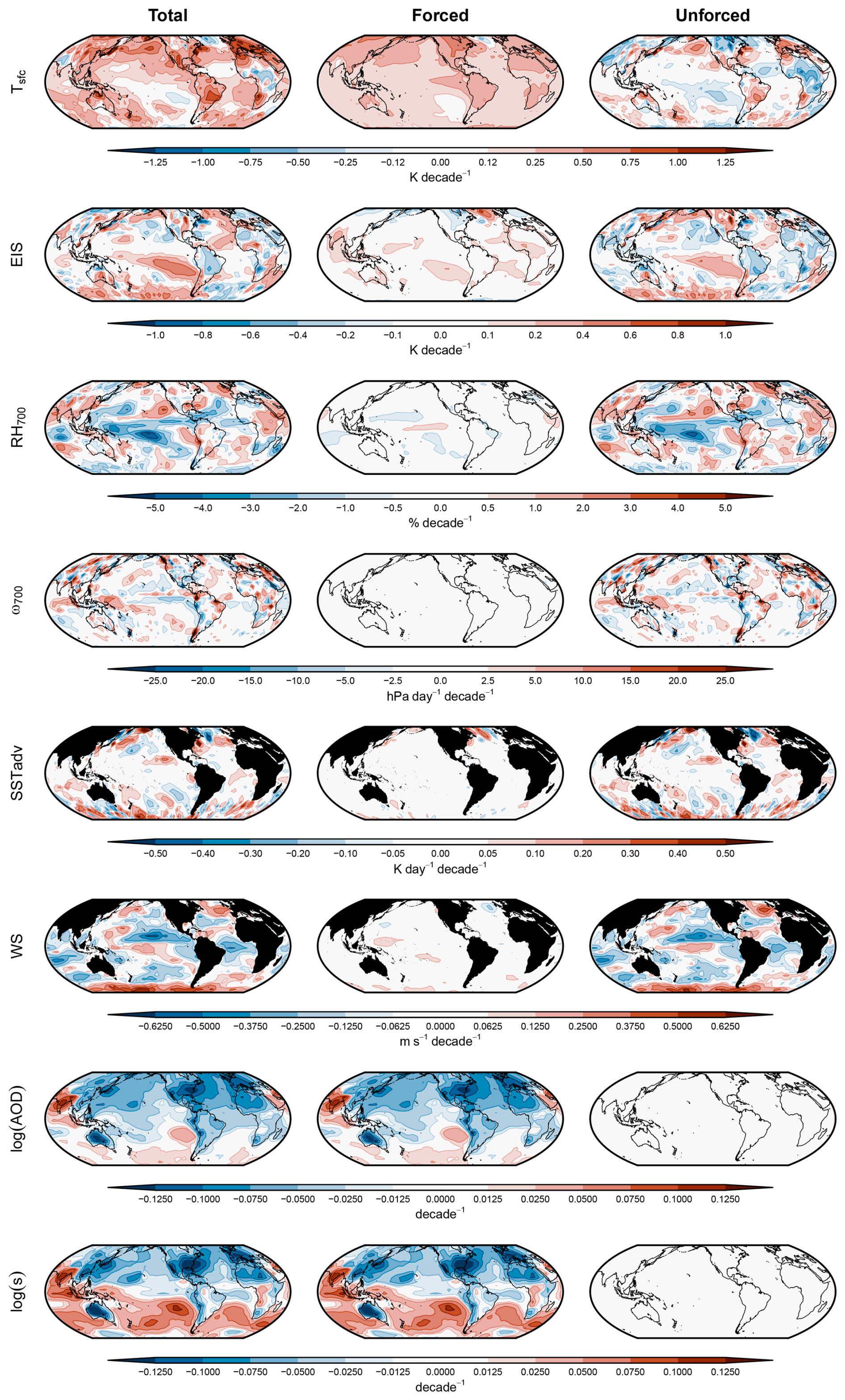
Figure A2 Maps of the decadal trends in each cloud-controlling factor (CCF), representing average values across all CCF datasets (Fig. A4).

A4.2 Radiative trend decomposition

We associate the aerosol adjustment contribution with the aerosol CCF trend, the cloud feedback contribution with the SST-mediated trend of the six meteorological CCFs, and the unforced variability contribution with the unforced CCF trends:

$$\begin{array}{}\text{(A5)}& \begin{array}{rl}& {\displaystyle \frac{{\mathrm{dSWCRE}}_{\mathrm{low}}}{\mathrm{d}t}}{|}_{\mathrm{aer}}\approx {\mathrm{\Theta }}_{\mathrm{aer}}\cdot {\displaystyle \frac{\mathrm{d}{X}_{\mathrm{aer}}}{\mathrm{d}t}},\\ & {\displaystyle \frac{{\mathrm{dSWCRE}}_{\mathrm{low}}}{\mathrm{d}t}}{|}_{\mathrm{fdbk}}\approx \sum _{i=\mathrm{1}}^{\mathrm{6}}{\mathrm{\Theta }}_i\cdot {\displaystyle \frac{\mathrm{d}{X}_i}{\mathrm{d}t}}{|}_{\mathrm{SST}},\\ & {\displaystyle \frac{{\mathrm{dSWCRE}}_{\mathrm{low}}}{\mathrm{d}t}}{|}_{\mathrm{unf}}\approx \sum _{i=\mathrm{1}}^{\mathrm{6}}{\mathrm{\Theta }}_i\cdot {\displaystyle \frac{\mathrm{d}{X}_i}{\mathrm{d}t}}{|}_{\mathrm{unf}},\end{array}\end{array}$$

where Θ is the cloud-radiative sensitivity, subscript “aer” represents either aerosol CCF, and we have ignored spatial indices for readability.

For GHG adjustments (Figs. 3f and A3), instead of using CCF analysis as per Eq. (A5), we rely entirely on model simulations: contrary to theoretical and modelling evidence of a moderate positive SWCRE_low adjustment (Andrews et al., 2012), CCF analysis predicts a weakly negative response (not shown), potentially because downwelling longwave radiation at the top of the boundary layer is not among our set of controlling factors. We proceed in the exact same way as for the calculation of $\frac{\mathrm{d}X}{\mathrm{d}t}{|}_{\mathrm{GHG}}$ above, but using SWCRE_low instead of CCF X.

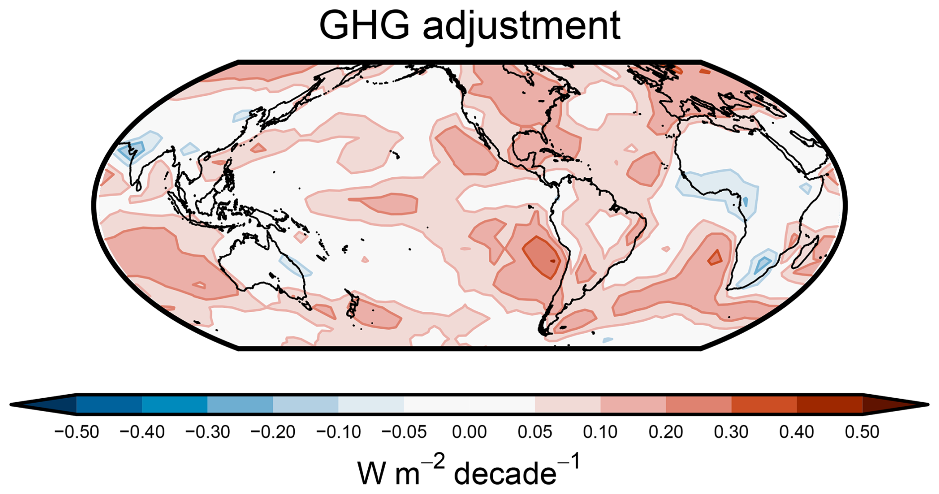
Figure A3 Contribution of GHG adjustments to the SWCRE_low trend, as in Fig. 3f but with a more finely resolved colourbar.

Several assumptions and limitations apply to our trend decomposition method. First, we assume that the CCF changes congruent with global-mean temperature represent a response to the forcing, i.e. a feedback. The method further assumes that CMIP6 models realistically capture the forced response pattern of SST and other variables, as well as the cloud adjustment to GHG. Evidence suggests models may be biased in their representation of present-day forced response patterns (e.g., Wills et al., 2022; Simpson et al., 2025), so the numbers based on our decomposition should be interpreted with caution. Note that, if the real-world forced CCF trends were closer to observed than to CMIP6-simulated trends, our decomposition method would by design yield an even smaller unforced SWCRE_low trend component.

A5 Uncertainty quantification

Trend confidence ranges include three sources of uncertainty, assumed mutually independent:

• First, we account for observational uncertainties in the CCFs, treating the two most uncertain CCFs, namely EIS and aerosol, separately from the rest (Appendix A6 and Figs. A4 and A5). We thus perform our observational CCF analysis with all possible combinations of five EIS estimates, four aerosol estimates (log(AOD) or log(s) from either CAMS or MERRA2), and two estimates for the remaining set of CCFs (ERA5 or MERRA2). This yields a 40-member ensemble of CCF sensitivities and thus radiative trend contributions from Eq. (A5). The standard deviations of these ensembles are denoted σ_obs,aer, σ_obs,fdbk, σ_obs,unf for the aerosol adjustment, cloud feedback, and unforced variability components of the trend, respectively (Appendix A4.2).

• Second, for the GHG adjustment trend we take the spread in CMIP6 model-simulated GHG low-cloud radiative adjustment, σ_mod,GHG, as a measure of uncertainty, using eight models with available data (Table A1).

• Third, we account for uncertainty in the decomposition between forced, SST-mediated and unforced components of the CCF and radiative trends, i.e. between $\frac{\mathrm{d}{X}_i}{\mathrm{d}t}{|}_{\mathrm{SST}}$ and $\frac{\mathrm{d}{X}_i}{\mathrm{d}t}{|}_{\mathrm{unf}}$, and hence $\frac{{\mathrm{dSWCRE}}_{\text{low}}}{\mathrm{d}t}{|}_{\mathrm{fdbk}}$ and $\frac{{\mathrm{dSWCRE}}_{\mathrm{low}}}{\mathrm{d}t}{|}_{\mathrm{unf}}$ (Eqs. A4–A5). Note that the same uncertainty applies to $\frac{{\mathrm{dSWCRE}}_{\mathrm{low}}}{\mathrm{d}t}{|}_{\mathrm{fdbk}}$ and $\frac{{\mathrm{dSWCRE}}_{\mathrm{low}}}{\mathrm{d}t}{|}_{\mathrm{unf}}$, since $\frac{\mathrm{d}{X}_i}{\mathrm{d}t}{|}_{\mathrm{unf}}$ is calculated as a residual (Appendix A4.1). We use the spread in forced responses among CMIP6 models as a measure of this uncertainty. Ideally, this spread would be obtained from multiple large ensembles from each CMIP6 model – where each model's ensemble-mean trend approximates the model's forced response. Since we only have a single realisation per model, we instead use bootstrapping: we generate 1000 synthetic 30-member ensembles of $\frac{{\mathrm{dSWCRE}}_{\mathrm{low}}}{\mathrm{d}t}{|}_{\mathrm{fdbk}}$, by randomly resampling (with replacement) $\frac{\mathrm{d}{X}_i}{\mathrm{d}t}{|}_{\mathrm{SST}}$ among 30 CMIP6 models (Table A1), while holding the CCF sensitivities fixed to their ensemble-mean values (Eq. A5). We then calculate ensemble means for each of the 1000 bootstrapped ensembles, and use the spread across these bootstrapped ensemble means as a measure of uncertainty for $\frac{{\mathrm{dSWCRE}}_{\mathrm{low}}}{\mathrm{d}t}{|}_{\mathrm{fdbk}}$ and $\frac{{\mathrm{dSWCRE}}_{\mathrm{low}}}{\mathrm{d}t}{|}_{\mathrm{unf}}$. Since it is derived from climate model spread in CCF trends, this uncertainty is denoted σ_mod,CCF.

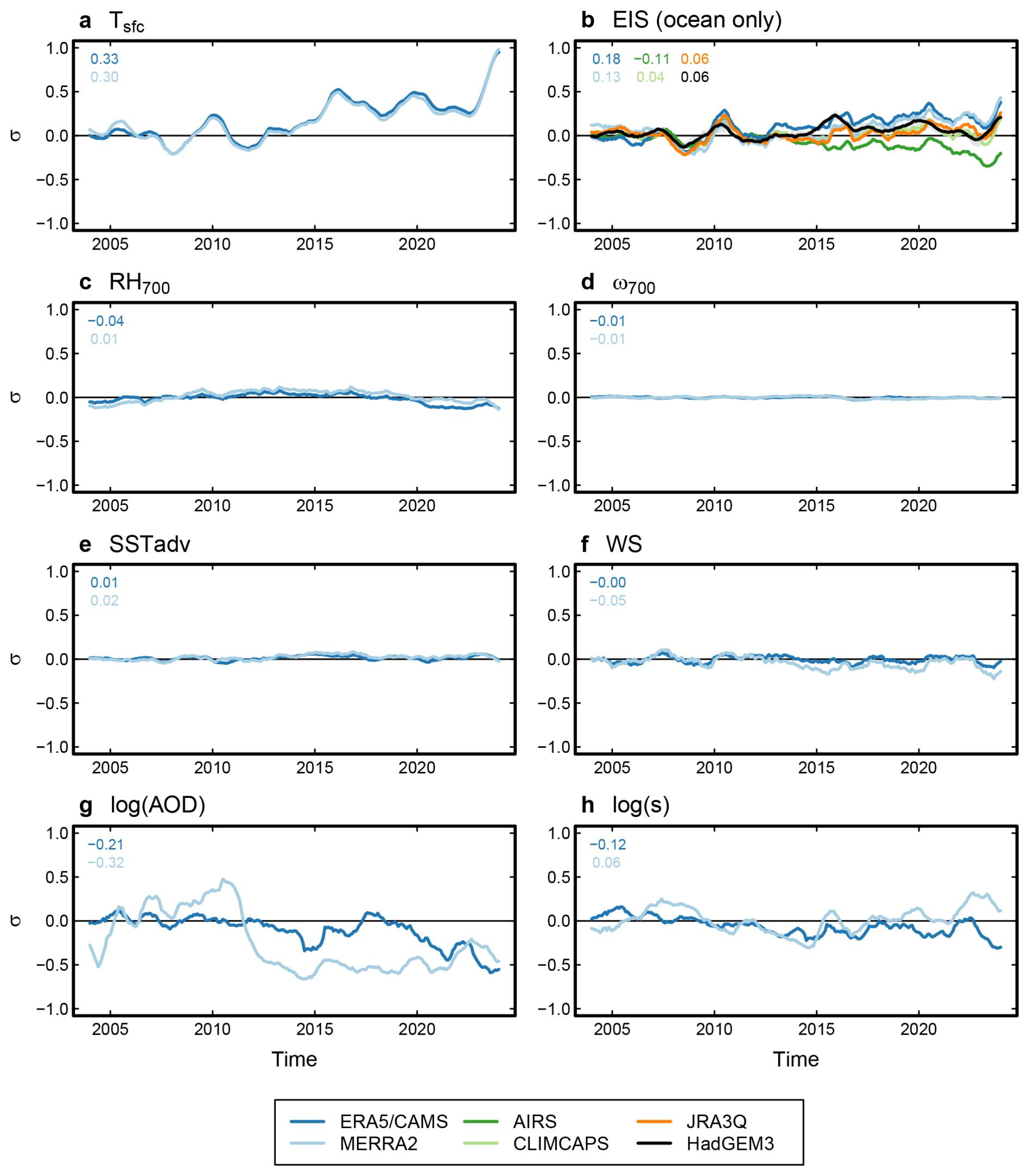
Figure A4 (a–h) Observational estimates of cloud-controlling factor (CCF) anomalies. Timeseries show standardised, deseasonalised monthly anomalies relative to the mean of the first 10 years, smoothed with a 12-month centred running mean; decadal trend values (in σ per decade) are shown in the top left corner of each panel. For each variable, the standardisation is done using the ERA5 or CAMS standard deviation, so that the magnitudes are comparable across datasets. Values are near-global averages (60° S to 60° N). In (b), in addition to four observational estimates, we include values simulated by a five-member ensemble of extended amip simulations with the HadGEM3 climate model (not used in the CCF analysis). The HadGEM3 ensemble mean is shown in thick black, with grey shading denoting the ensemble range.

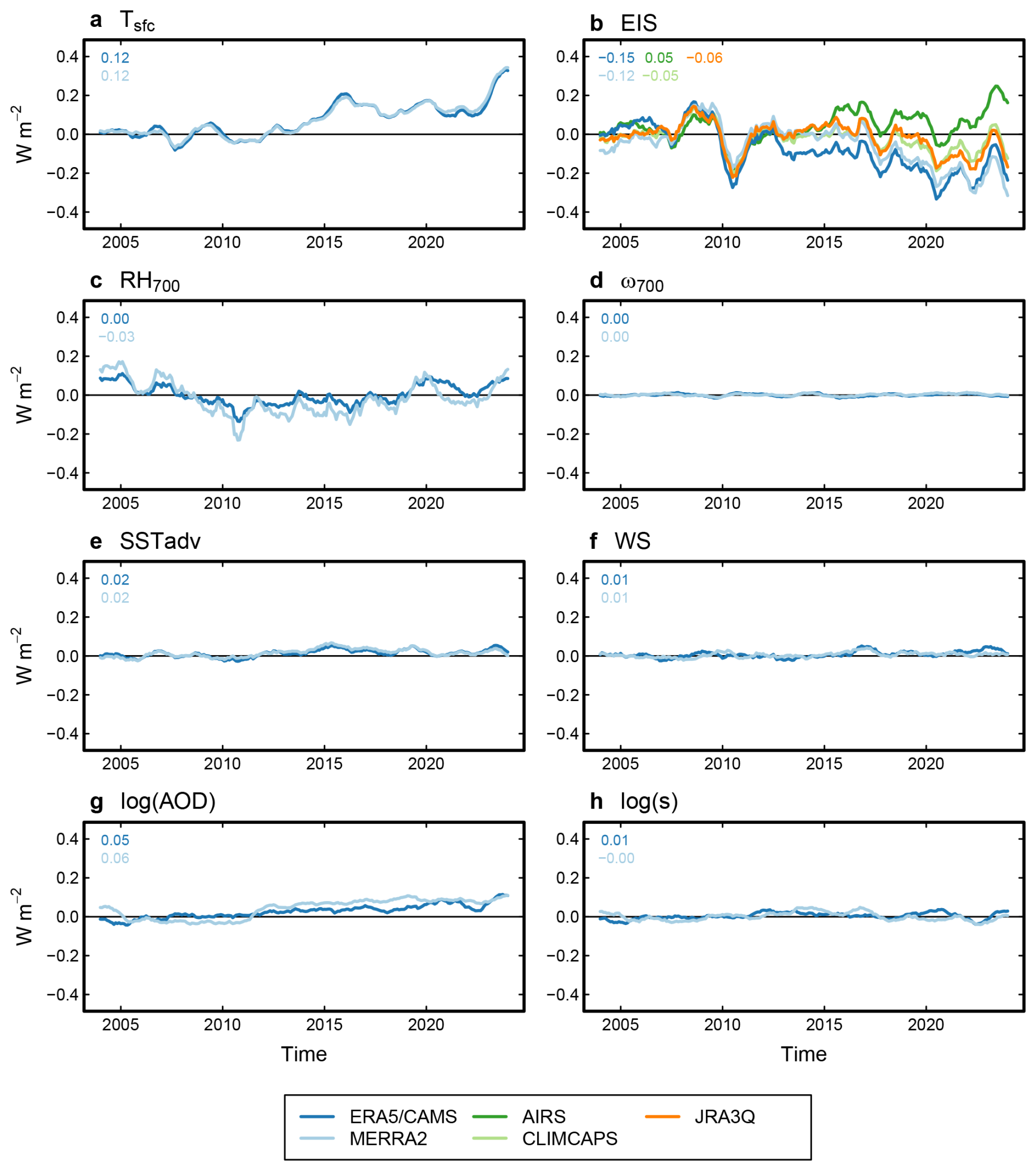
Figure A5 (a–h) As in Fig. A4, but showing the contributions of each CCF dataset to the near-global SWCRE_low anomalies, calculated relative to the mean of the first 10 years. Decadal trend values (in W m⁻² per decade) are shown in the top left corner of each panel. Curves are averages over the corresponding ensemble members: for example, the dark blue curve in (a) is an average over estimates based on every possible combination of five EIS datasets, four aerosol datasets, and ERA5 data for the remaining five CCFs, yielding 20 ensemble members.

The overall uncertainties in the trend components (Fig. 1d) are then quantified as follows:

• For $\frac{{\mathrm{dSWCRE}}_{\mathrm{low}}}{\mathrm{d}t}{|}_{\mathrm{aer}}$, from observational CCF uncertainty: ${\mathit{\sigma }}_{\mathrm{aer}}={\mathit{\sigma }}_{\mathrm{obs},\mathrm{aer}}$.

• For $\frac{{\mathrm{dSWCRE}}_{\mathrm{low}}}{\mathrm{d}t}{|}_{\mathrm{GHG}}$, from the spread in CMIP6 trends in low-cloud adjustment, σ_mod,GHG.

• For $\frac{{\mathrm{dSWCRE}}_{\mathrm{low}}}{\mathrm{d}t}{|}_{\mathrm{fdbk}}$ and $\frac{{\mathrm{dSWCRE}}_{\mathrm{low}}}{\mathrm{d}t}{|}_{\mathrm{unf}}$, as the sum (in quadrature) of the observational CCF uncertainty, and the uncertainty from the model-based decomposition of the CCF trends: ${\mathit{\sigma }}_{\mathrm{fdbk}}=\sqrt{{\mathit{\sigma }}_{\mathrm{obs},\mathrm{fdbk}}^{\mathrm{2}}+{\mathit{\sigma }}_{\mathrm{mod},\mathrm{CCF}}^{\mathrm{2}}}$; ${\mathit{\sigma }}_{\mathrm{unf}}=\sqrt{{\mathit{\sigma }}_{\mathrm{obs},\mathrm{unf}}^{\mathrm{2}}+{\mathit{\sigma }}_{\mathrm{mod},\mathrm{CCF}}^{\mathrm{2}}}$.

• For $\frac{{\mathrm{dSWCRE}}_{\mathrm{low}}}{\mathrm{d}t}{|}_{\mathrm{for}}$, as the sum (in quadrature) of the uncertainties in $\frac{{\mathrm{dSWCRE}}_{\mathrm{low}}}{\mathrm{d}t}{|}_{\mathrm{fdbk}}$, $\frac{{\mathrm{dSWCRE}}_{\mathrm{low}}}{\mathrm{d}t}{|}_{\mathrm{aer}}$ and $\frac{{\mathrm{dSWCRE}}_{\mathrm{low}}}{\mathrm{d}t}{|}_{\mathrm{GHG}}$: ${\mathit{\sigma }}_{\mathrm{for}}=\sqrt{{\mathit{\sigma }}_{\mathrm{fdbk}}^{\mathrm{2}}+{\mathit{\sigma }}_{\mathrm{aer}}^{\mathrm{2}}+{\mathit{\sigma }}_{\mathrm{GHG}}^{\mathrm{2}}}$.

• Finally, for the total reconstructed trend, as the sum (in quadrature) of the uncertainties in $\frac{{\mathrm{dSWCRE}}_{\mathrm{low}}}{\mathrm{d}t}{|}_{\mathrm{for}}$ and $\frac{{\mathrm{dSWCRE}}_{\mathrm{low}}}{\mathrm{d}t}{|}_{\mathrm{unf}}$, but ensuring σ_mod,CCF is not double-counted: ${\mathit{\sigma }}_{\mathrm{reconstructed}}=\sqrt{{\mathit{\sigma }}_{\mathrm{for}}^{\mathrm{2}}+{\mathit{\sigma }}_{\mathrm{unf}}^{\mathrm{2}}-{\mathit{\sigma }}_{\mathrm{mod},\mathrm{CCF}}^{\mathrm{2}}}$.

Uncertainty in the observed SWCRE_low trend is based on Raghuraman et al. (2021)'s uncertainty estimate of ±0.1 W m⁻² per decade (±1σ) for CERES global-mean trends. We apply this to the global SWCRE trend due to all cloud types, and assume that low and non-low clouds contribute equally and independently to this uncertainty. This results in a ±1σ range of $\pm \mathrm{0.1}/\sqrt{\mathrm{2}}=\pm \mathrm{0.07}$ W m⁻² per decade for the observed global SWCRE_low trend.

A6 Uncertainties in cloud-controlling factor trends

Reanalysis products suffer from known issues in their representation of long-term trends, introducing uncertainty in our analysis. To assess this uncertainty, in Fig. A4 we display the timeseries of near-global, standardised CCF anomalies. Figure A5 shows the corresponding radiative contributions, obtained per Eq. (A2).

The largest (standardised) trend uncertainties are in the EIS and aerosol CCFs (Figs. A4b, g, h and A5b, g, h). For EIS, given the reanalysis uncertainty we include three datasets in addition to ERA5 and MERRA2: an EIS estimate based on the JRA3Q reanalysis product; and two satellite-based estimates of 700 hPa temperature, T₇₀₀, from AIRS and CLIMCAPS, combined with ERA5 T_sfc. (Note that EIS is based upon the difference between T₇₀₀ and T_sfc, and T_sfc trends are well-constrained per Fig. A4a.) The five observational estimates of EIS disagree on the sign of the trend, ranging from −0.12σ per decade (AIRS) to +0.16σ per decade (ERA5). To provide additional context for these trends, we analyse an extended, five-member amip experiment with historical forcings up to 2014 and SSP2-4.5 from 2015 onwards, where SSTs and sea ice are taken from HadISST1 (Rayner et al., 2003). The HadGEM3 simulations yield an ensemble-mean EIS trend of +0.04σ per decade, in the middle of the observational uncertainty range. While HadGEM3 may misrepresent aspects of the physics relevant to the EIS trend, the model's atmospheric state is known perfectly and hence there is no observational uncertainty. The HadGEM3 result thus provides some confidence that the “true” EIS trend lies within the observational uncertainty range.

For the aerosol CCF, the two reanalysis products used here, CAMS and MERRA2, show distinct time evolutions of sulphate AOD and mass concentration s (Fig. A4g and h), reflecting substantial observational uncertainty. While CAMS exhibits a relatively gradual log(AOD) decrease, with a trend of −0.19σ per decade, MERRA2 shows a much more abrupt decline in the early 2010s, with a stronger linear trend of −0.37σ per decade. By contrast, the log(s) trends are much weaker, with MERRA2 even reporting a weakly increasing global trend of +0.06σ per decade. The differences in the sign of the global sulphate aerosol trend reflect observational uncertainty in the magnitude of the sulphate aerosol increase in the Southern Hemisphere (Fig. A2), which has been attributed to wildfires and volcanoes (Park and Soden, 2025).