Snow microphysical processes in orographic turbulence revealed by cloud radar and in situ snowfall camera observations

Turbulence influences snow microphysics and precipitation formation, while simultaneously degrading polarimetric radar measurements through broadening of the canting angle distribution. We investigate these interactions in the Colorado Rocky Mountains, where an orographic turbulent layer consistently forms in the lee of Gothic Mountain during precipitation events. To isolate microphysical signals from turbulence-induced artifacts, we apply a novel framework contrasting radar observations above and below the turbulent layer. The dataset combines polarimetric W-band and collocated Ka-band radar measurements with surface in situ observations from the Video In Situ Snowfall Sensor (VISSS). All observations were collected during the CORSIPP project, part of the ARM SAIL campaign (winter 2022/2023).

Aggregation is identified as a dominant process within the turbulent layer, occurring primarily between −12 and −15 °C. It is responsible for reflectivity (Z_e) increase of up to 20 dBZ km⁻¹ and reduction of the mean particle fall velocity. Enhanced K_DP and $\mathrm{s}{Z}_{{\mathrm{DR}}_{\max }}$ further suggest secondary ice production through ice-collisional fragmentation, generating anisotropic splinters. Riming also occurs frequently, with Z_e increases up to 15 dBZ km⁻¹ and systematically increasing mean particle fall velocity. Riming inside the turbulent layer was often observed at temperatures below −10 °C, indicating the presence of supercooled liquid at cold conditions. Statistical analysis revealed that the turbulent layer is frequently collocated with supercooled liquid water layers near the Gothic Mountain summit.

Our findings demonstrate how radar polarimetry may be safely used to investigate microphysical processes inside a turbulent layer and highlight the impact of orographic turbulence on snow microphysics and precipitation enhancement.

1 Introduction

Mountainous regions play a central role in the earths water budget, acting as the Earth's water towers, and are especially vulnerable to changes in the amount of precipitation (e.g Li et al., 2023, and references therein). Understanding precipitation generation and distribution in mountainous regions depends on understanding the microscale dynamics and microphysics that transform condensed water into precipitation.

In the context of precipitation formation in mountainous regions, turbulence has been a key area of research in recent years. Turbulence in mountainous areas frequently occurs due to wind shear, which involves a significant variation in wind speed and/or direction across a small vertical distance. This may for example occur at the interface between a blocked low level flow inside a valley and the unblocked cross-barrier flow aloft (e.g. Ramelli et al., 2021; Kötsche et al., 2025). Blocking caused by mountains is a very complex topic and further insight may be found in the work of, for example, Smolarkiewicz and Rotunno (1989) and Smolarkiewicz and Rotunno (1990). Along the flanks of a blocking mountain, a tip jet can form which features enhanced wind speeds and hence wind shear. Downstream of the blocking mountain, a wake, recirculating flow or general deceleration of the wind is found (Petersen et al., 2005). This recirculating or converging flow in the lee of blocking mountains also leads to pronounced moisture convergence (e.g. Bhushan and Barros, 2007), which consequently may lead to cloud and precipitation formation.

Various studies in recent years focused on the implications of turbulence on precipitation formation. Lee et al. (2014) demonstrated that turbulence boosts supersaturation, leading to faster ice crystal growth through deposition. Additionally, ice particles collide more effectively with supercooled droplets, enabling them to grow into small graupel particles. Consequently, turbulence leads to a relatively large number of small-sized graupel particles. Aikins et al. (2016) also argued that in cold post frontal continental environments (temperatures below −15 °C), turbulence plays a significant role in promoting snow growth mainly via deposition and aggregation. Houze and Medina (2005), Houze (2012) and Medina and Houze (2015) discovered that turbulent updraft cells can generate areas of elevated liquid water content (LWC), which promote riming and coalescence while also enhancing aggregation due to variations in the particle fall velocities. Grazioli et al. (2015) presented measurements gathered in an inner-Alpine valley, they confirmed that if a turbulent layer persists for several hours, sustaining supercooled liquid water (SLW) production, it prolongs riming and allows for large snow accumulations at ground level. Conversely, Aikins et al. (2016) found no SLW near the turbulent cells when conducting measurements in the Sierra Madre Range in Wyoming. They suggested that the absence of liquid water is likely because the high concentration of ice particles from the cloud above rapidly depletes water vapor, preventing liquid drop formation. Ramelli et al. (2021), consistent with previous studies, reported changes in the microphysical characteristics of clouds in the turbulent shear layer. These modifications included alterations in particle shape or density and increased ice growth. Similar to Grazioli et al. (2015), their measurements were conducted within an inner-Alpine valley. They furthermore speculate that collisions of fragile ice crystals with large rimed ice particles act as a secondary ice production (SIP) mechanism. Billault-Roux et al. (2023) also reported new ice formation associated with updrafts and turbulence within the Swiss Jura Mountains. They concluded that turbulence and updraft favor riming and SIP through ice–ice collisions of these newly rimed particles. Chellini and Kneifel (2024) analysed a long-term dataset collected at AWIPEV observatory in Ny-Ålesund. They discovered that higher eddy dissipation rate (EDR) as a measure of in-cloud turbulence is associated with increasing size of ice particles at dendritic-growth temperatures and likely also aids increasing SIP via fragmentation of dendritic structures. For temperatures above −10 °C, Chellini and Kneifel (2024) found that turbulence increases riming rates, suggesting that riming in shallow liquid layers is a fundamentally turbulent process. Evidence of SIP through ice-collisional fragmentation in connection with an orographic turbulent layer was also reported in Kötsche et al. (2025).

While many studies have highlighted riming, aggregation, and secondary ice production (SIP) as key processes in turbulent layers, they often relied on case studies (Grazioli et al., 2015; Aikins et al., 2016; Billault-Roux et al., 2023; Kötsche et al., 2025) or datasets with limited temporal coverage (Medina and Houze, 2015). Furthermore, direct, collocated in situ validation of hydrometeor type and shape remains rare in remote sensing studies. Finally, turbulence is causing particles to be more randomly oriented and is hence increasing the width of the canting angle distribution of particles (Klett, 1995; Garrett et al., 2015). Polarimetric radar variables such as differential reflectivity (Z_DR) and specific differential phase (K_DP) are depended on the width of the canting angle distribution (Ryzhkov et al., 2002; Hubbert and Bringi, 2003; Ryzhkov and Zrnic, 2019), hence more turbulence means lower magnitudes of Z_DR and K_DP (e.g., Kötsche et al., 2025). Turbulence can degrade the interpretability of polarimetric signals as well as inhibit the use of radar Doppler spectra based retrieval techniques, effectively “blinding” radars within turbulent layers. This aspect has, in our opinion, not received sufficient attention in previous studies.

In this study, we focus on characterizing an orographic turbulent layer and the microphysical processes therein for a field site in the Colorado Rocky Mountains utilizing long-term measurements of a slanted dual-polarimetric W-band radar (LIMRAD94, model RPG-FMCW-94-DP; Küchler et al., 2017), collocated with the Video In Situ Snowfall Sensor (VISSS, Maahn et al., 2024b) and the single-polarization Ka-band ARM Zenith Radar (KAZR, Widener et al., 2012). To overcome the “blinding” effect of turbulence on polarimetric Doppler radar observations, we do not analyze data from inside the turbulent layer, but rather compare variables above and below the turbulent layer to then draw conclusions on the microphysical processes inside it. The collocated VISSS data provides valuable insights into the properties of the observed hydrometeor populations including rime mass fraction. The data collection was conducted under the Characterization of Orography-influenced Riming and Secondary Ice production and the associated impact on Precipitation rates using radar Polarimetry and Doppler spectra (CORSIPP) project, a component of the DFG Priority Programme SPP-PROM (Trömel et al., 2021). CORSIPP was integrated into the Atmospheric Radiation Measurement (ARM) Surface Atmosphere Integrated Field Laboratory (SAIL) campaign (Feldman et al., 2023) for which the AMF2 was deployed during the exceptionally snowy winter of 2022/2023 in the Colorado Rocky Mountains. The measurement site at Gothic, next to Gothic Mountain, is strongly influenced by turbulence and hence prompts us to examine turbulence's effects on precipitation formation. LIMRAD94, VISSS, and KAZR data are further supplemented by other nearby remote sensing and in situ instruments deployed during SAIL.

In Sect. 2, we describe the instruments, data, and methods utilized in this study. The SWL layer detection, EDR retrieval, turbulent layer formation and turbulent layer detection are explained in Sect. 2.4, 2.5, 2.6, and 2.6.1, respectively. The novel methodology developed to derive microphysical processes inside the turbulent layer is presented in Sect. 2.6.2. The results and discussion Section (Sect. 3) contains a statistical evaluation of the turbulent layer (Sect. 3.1) and an analysis of fingerprints of microphysical processes in the turbulent layer (Sect. 3.2). The summary and conclusion can be found in Sect. 4.

2 Data and Methods

In the following sections, the instruments used for this study and their respective variables are described. We provide an overview of the retrievals for the eddy dissipation rate (EDR), the liquid layer using lidar data, and the turbulent layer height (TLH). Additionally, we present the methodology for deriving microphysical processes inside the turbulent layer.

2.1 Radars

2.1.1 Overview

Throughout CORSIPP, the dual-polarimetric W-band radar (LIMRAD94, model RPG-FMCW-94-DP; Küchler et al., 2017) was operated within a cold-temperature scanning unit. This installation took place at an elevation of 2905 m at the Rocky Mountain Biological Laboratory (RMBL), approximately 525 m from the second ARM Mobile Facility (AMF2) in Gothic, Colorado. LIMRAD94 was positioned near the RMBL Ore House from 15 November 2022, to 5 June 2023. Observations with LIMRAD94 were made at a fixed elevation of 40° and at an azimuth angle of 151° pointing towards the VISSS and the AMF2 as illustrated in Fig. 1. For additional technical specifics regarding the deployment of LIMRAD94 and VISSS during CORSIPP, please refer to Kalesse-Los et al. (2023a) and Kötsche et al. (2025). As part of SAIL, the ARM KAZR (Widener et al., 2012) was stationed at the AMF2 at 2889 m above mean sea level (a.m.s.l.). Also, a scanning dual polarization X-band radar (CSU X-band) from Colorado State University (CSU) was deployed in a distance of 8018 m (at 149° azimuth, 3147 m a.m.s.l.) from LIMRAD94 (also see Appendix B, Fig. B1). From the CSU X-band radar data, RHI scans at 329° azimuth (towards the AMF2 and LIMRAD94) and plane position indicator (PPI) scans at 4° elevation were used in Fig. 3. Additionally, the ARM 915 MHz Radar Wind Profiler (RWP915, Muradyan and Coulter, 2020) was installed at the AMF2 in November 2022, providing profiles of horizontal and vertical wind with a resolution of 1 h.

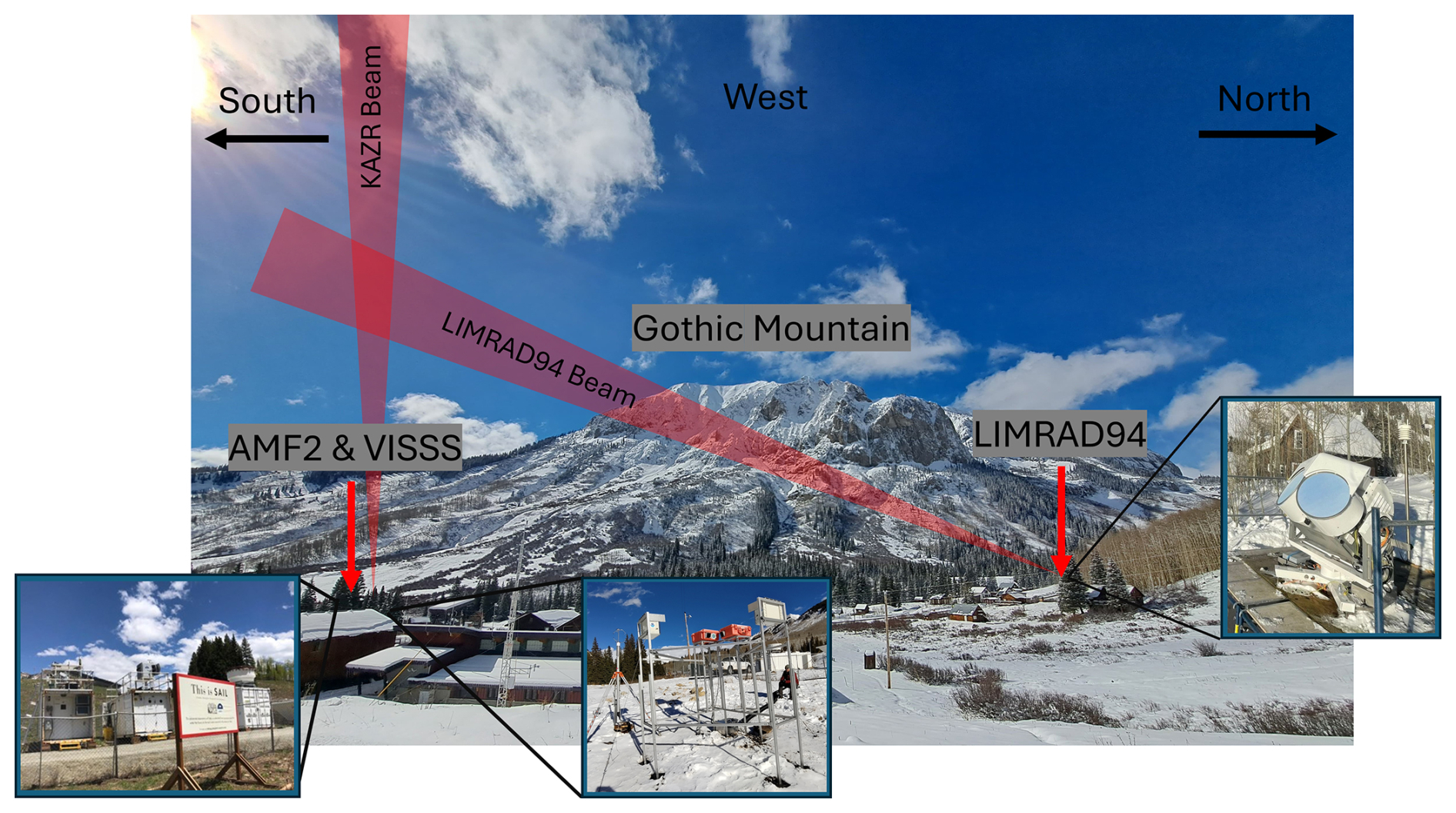
Figure 1 The primary measurement site (Gothic, Colorado) during the second winter of the SAIL campaign 2022/23, where the CORSIPP project was conducted.

2.1.2 Polarimetric radar data

LIMRAD94 has the capability to measure spectral polarimetric variables such as differential phase shift and differential reflectivity, among others. The polarimetric calibration for LIMRAD94 was conducted at the onset of the field campaign, coinciding with a period of vertically oriented measurements as outlined in Myagkov et al. (2016).

The differential phase shift Φ_DP (°) consists of a backscatter and a propagational part, where the propagational part is called specific differential phase K_DP (° km⁻¹). We calculated K_DP from Φ_DP using a convolution with low-noise Lanczos differentiators with a window length of 23 gates. This method is implemented in the python package wradlib (Heistermann et al., 2013).

Backscatter differential phase (δ) is caused by hydrometeors large enough relative to the radar wavelength such that the scattering is in the non-Rayleigh regime (Trömel et al., 2013). δ was found to be negligible for frozen hydrometeors in the S, C, and X-bands (Balakrishnan and Zrnic, 1990; Ryzhkov et al., 2011; Trömel et al., 2013). In the data of our W-band radar however, we find a contribution of δ, predominantly during cases with large graupel. Because removing the δ contribution from Φ_DP is not easy to perform, we chose to omit radar data where δ is occurring. δ causes so called bumps, sudden increases in Φ_DP followed by a decrease. This results in negative K_DP values, which are therefore a good indicator for δ. We defined δ to be present if K_DP in a radar range gate is below −0.5 ° km⁻¹, Z_e is higher than 0 dBZ and SNR is above 10 dB. We then removed all profiles where more than 10 range gates fulfilled the δ criterion. We acknowledge that the thresholds selected for the removal of δ are empirical and based on observations from instances where we noted the contribution of backscatter differential phase in our data. The method enables us to drop the majority of δ contaminated data, but the thresholds may not be directly applicable to other radar data. To the authors knowledge, there is currently no other literature available that addresses the removal of δ in snow at W-band. The approach described in Myagkov et al. (2020), which utilizes Doppler spectra in low turbulence conditions and was demonstrated during rain is not applicable in our case. It would be desirable for future publications to develop a solid method to remove the δ contribution from Φ_DP in snow directly, before calculating K_DP.

K_DP depends on the shape, orientation, concentration, density and the size of hydrometeors. Elevated concentrations of dense ice particles that exhibit greater anisotropy in shape and possess uniform orientation result in increased values of K_DP. It was furthermore shown by Kötsche et al. (2025) that up to 20 % of W-band K_DP can be attributed to aggregates. Additionally, K_DP is affected by turbulence due to its reliance on the width of the canting angle distribution (σ) as shown by Ryzhkov et al. (2002) and Ryzhkov and Zrnic (2019). As turbulence intensifies, the magnitude of σ increases, consequently leading to a reduction in K_DP.

The differential reflectivity Z_DR (dB) is commonly defined as the ratio between the radar reflectivity measured at horizontal polarization and at vertical polarization. At W-band, the largest contribution to elevated Z_DR values in the ice phase typically comes from dense, anisotropic ice crystals that are small enough to be within the Rayleigh scattering regime, and often found on the slower side of the radar Doppler spectrum. Unlike K_DP, Z_DR is immune to the total concentration factor. Spherical and/or less dense particles result in a reduced Z_DR. Since Z_DR is reflectivity-weighted, its magnitude is often reduced by larger, spherical particles (e.g., Oue et al., 2018). To avoid this masking issue when using Z_DR, we also determine the maximum spectral Z_DR value ($\mathrm{s}{Z}_{{\mathrm{DR}}_{\max }}$) for each Doppler spectrum. Similar to K_DP, overall Z_DR values are reduced by turbulence through an increased width of the canting angle distribution. $\mathrm{s}{Z}_{{\mathrm{DR}}_{\max }}$ is furthermore reduced by broadening of the Doppler spectrum caused by turbulence. More detailed descriptions of these polarimetric variables and the influence of turbulence on them can be found in Kötsche et al. (2025).

2.2 VISSS

The first generation VISSS was installed next to the AMF2 facility, in the line of sight of LIMRAD94 with a horizontal distance to LIMRAD94 of approximately 550 m (Fig. 1). VISSS1 has a pixel resolution of 58.832 µm px⁻¹, a frame rate of 140 Hz, and an observation volume of 75.2 × 75.2 × 60.1 mm³ (Maahn et al., 2024b). This yields an observational volume of 0.000339 m³. VISSS level2match variables (see Fig. 2 in Maahn et al., 2024b) used in this study include particle size distributions (PSD), D₃₂, complexity, and total number concentration (N_tot). D₃₂ is the ratio of the third to the second measured PSD moment. Assuming that particle mass is proportional to the particle maximum dimension squared, D₃₂ is a proxy for the mass-weighted mean diameter of the particle population (Maahn et al., 2015). Following Schmitt and Heymsfield (2014), the complexity c is derived from the ratio of the particle perimeter p to the perimeter of a circle with the same area A:

$$\begin{array}{}\text{(1)}& c={\displaystyle \frac{p}{\mathrm{2}\sqrt{\mathit{\pi }A}}}.\end{array}$$

The complexity can be used to distinguish between ice particle habits as for example demonstrated in Garrett and Yuter (2014).

2.3 Additional data products

Vertical temperature profiles on site are provided by the ARM interpolated sonde and gridded sonde value added product (Fairless et al., 2021). For the processing, ARM uses sounding data collected on site through two radiosonde launches per day (11:00 and 23:00 UTC). They then transform the data into continuous daily files with 1 min time resolution and combined with ARM 3-channel microwave radiometer precipitable water vapor data. Data from the high resolution spectral lidar (HSRL) installed at AMF2 (Goldsmith, 2016) was used to detect SLW. Particle number concentrations for the whole SAIL campaign period were measured by the ARM Laser Distrometer (Bartholomew, 2020), an OTT Parsivel2 (from now on referred to as Parsivel2). The cloud base height was retrieved by the ARM ceilometer (Morris, 2016). Rime mass fraction M was calculated using VISSS particle size distributions (PSD) and LIMRAD94 Z_e with the approach of Maherndl et al. (2024, 2025).

2.4 Liquid layer detection

A liquid layer was detected when the HRSL attenuated backscatter coefficient at 1064 nm exceeded $>\mathrm{1}\times {\mathrm{10}}^{-\mathrm{5}}$ m⁻¹ sr⁻¹ and the linear depolarization ratio was <0.05, as the depolarization of water droplets should be close to 0 according to Vaisala (2021). The lidar data was filtered using a signal to noise ratio threshold of 10 dB. In the following, we use LLB to refer to the liquid-containing layer base height. We acknowledge that the LLB will generally be consistent with the ceilometer-derived cloud base height, since both instruments detect liquid layers as proxies for cloud base. Nevertheless, retrieving the LLB directly from HSRL adds value: it provides an independent product for cross-validation with the ceilometer, and it allows cloud-base detection to be performed using only the HSRL data set. This ensures consistency for studies that rely exclusively on HSRL observations.

2.5 Turbulence eddy dissipation rate retrieval (EDR)

As a proxy for atmospheric turbulence, the eddy dissipation rate EDR quantifies the rate at which turbulent kinetic energy is lost to viscous forces (Foken and Mauder, 2024). Elevated EDR values are associated with more intense turbulence. In this study, EDR was estimated from mean Doppler velocity (MDV) measurements obtained by KAZR, aggregated over five-minute intervals following the method outlined in Vogl et al. (2024). The original approach of the EDR calculation is based on Borque et al. (2016). To isolate regions of significant turbulence, we applied an empirical threshold of 10⁻³ m² s⁻³, consistent with the criterion used by Vogl et al. (2022). It is important to note that during the CORSIPP campaign, the radar beams of KAZR and LIMRAD94 were not perfectly aligned (Fig. 2). As a result, the volumes from which KAZR-EDR and LIMRAD94 measurements were collected are horizontally offset, with the separation increasing with altitude (580 m horizontal distance at Gothic Mountain summit height).

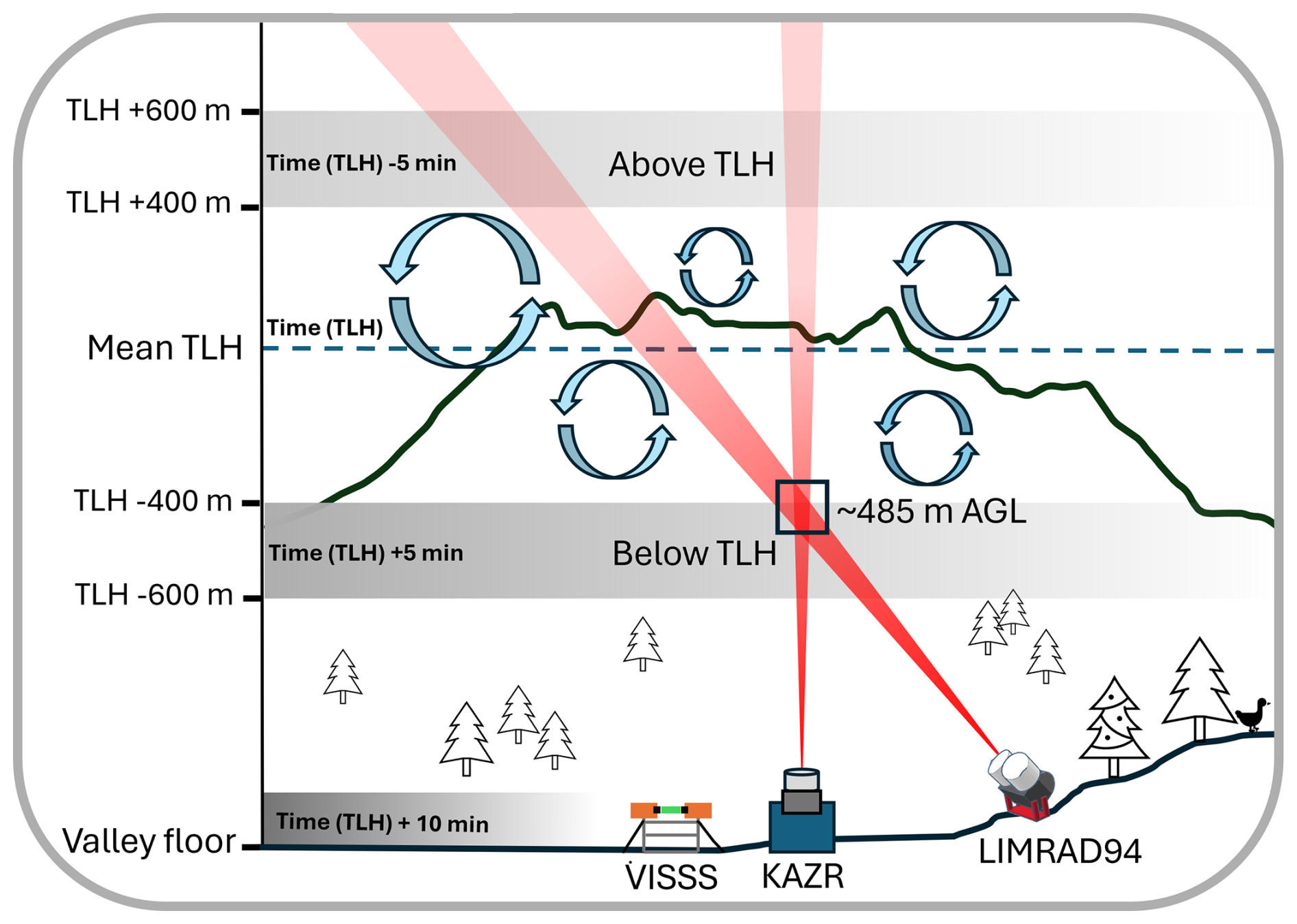
Figure 2 Methodology to analyze microphysical processes inside the turbulent layer described in Sect. 2.6.2. Shown is a schematic of the measurement site including LIMRAD94, KAZR, VISSS and their measurement volumes. Blue arrows indicate turbulence which most frequently occurs around the summit height of Gothic Mountain (black line in the background). The dashed blue line indicates the mean turbulent layer height. Grey areas above TLH and below TLH mark the area in which radar data are averaged to avoid contamination of the measurement volume by turbulence.

2.6 The turbulent layer

Due to the orography surrounding the measurement site, we observed a distinct layer of enhanced turbulence, predominantly at and below 1000 m above ground level (a.g.l.) and during south westerly to north westerly wind directions (details shown in Sect. 3.1). Gothic Mountain, a cone-shaped mountain located just west of the measurement site (see Fig. B1), is suspected to be the primary driver for the formation of this turbulent layer. To illustrate this, we will present an exemplary case study on 6 December 2022 where the formation mechanism of the turbulent layer is visible. This case study was previously described in Kötsche et al. (2025).

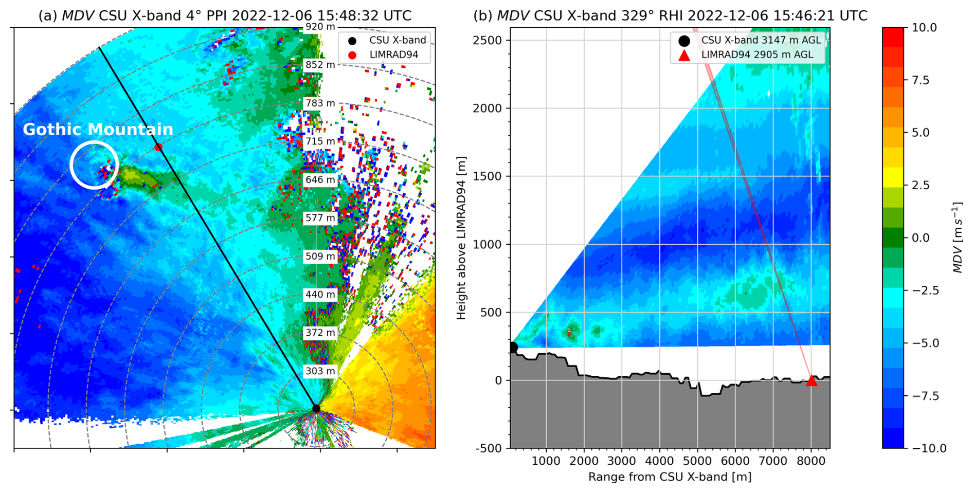
Figure 3 This figure was already presented in our previous study (Kötsche et al., 2025), we show it again to visualize the turbulent layer formation behind Gothic Mountain. (a) Mean Doppler velocity (i.e., the approximate radial component of the horizontal wind) from the CSU X-band PPI scan at a 4° elevation angle, showing the position of Gothic Mountain (white circle) and the RHI scan direction at an azimuth of 329° (black line) at 15:48:32 UTC on 6 December 2022. The map is displayed in a north-up orientation, with north at the top of the figure. Grey dashed circles mark every 1000 m in range from the CSU X-band. The labels indicate the corresponding heights of the CSU X-band radar beam above LIMRAD94. (b) Mean Doppler velocity from the CSU X-band RHI scan (azimuth 329°) at 15:46:21 UTC on 6 December 2022, with the LIMRAD94 beam direction shown in red. Grey shading represents the terrain elevation profile.

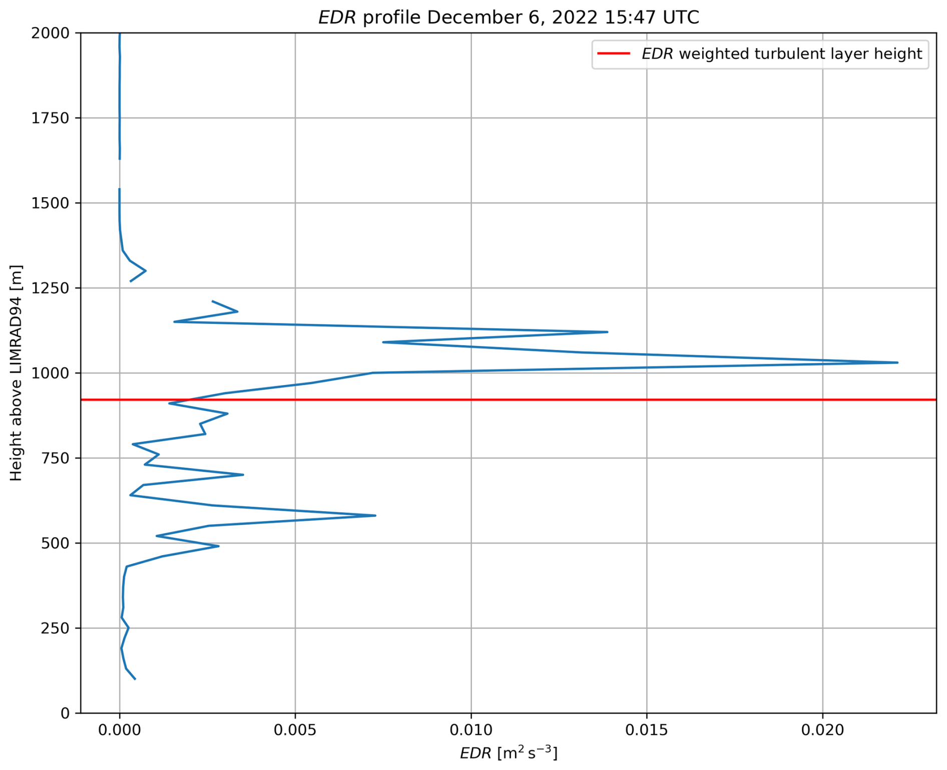
Figure 3 shows the MDV of CSU X-band from a PPI (panel a) and a RHI (panel b) scan at around 15:48 and 15:46 UTC, respectively. During that time, EDR indicates enhanced turbulence between 500 and 1200 m above LIMRAD94, with the mean EDR weighted turbulent layer height of 900–950 m (Fig. 4). The MDV observed in the PPI scan can be interpreted as the radial component of the horizontal wind. Negative values (blue) in Fig. 3 represent motion toward the radar, while positive values (yellow–red) indicate motion away from it. Although parts of the PPI are blocked by surrounding mountains, a prevailing westerly flow is evident from the blue shading west of the CSU X-band and the orange–red shading to the east. Where MDV approaches zero, the wind direction is nearly perpendicular to the radar beam. Downstream of Gothic Mountain, at approximately 700–800 m above LIMRAD94, a narrow band is observed in which MDV exhibits an abrupt transition to positive values, contrasting sharply with the surrounding negative values. This pattern indicates that, in the lee of Gothic Mountain, the wind veers toward a more southerly direction, though this effect weakens rapidly further downstream.

Figure 4 EDR profile and EDR weighted TLH as described in Sect. 2.6.1 in on 6 December 2022 15:47 UTC, roughly the same time the radar scans of CSU X-band in Fig. 3 were performed.

In the RHI scan (Fig. 3b), this southerly component is expressed as a region with predominantly green colors at ranges of 6000–7000 m from the CSU X-band and altitudes of 500–900 m above LIMRAD94. This disturbance is likely associated with a counterflow behind Gothic Mountain, suggesting blocked low-level flow, similar to the situations discussed in Ramelli et al. (2021). Enhanced wind shear is found along the upper and lower boundaries of this counterflow, likely producing the turbulence identified by EDR in Fig. 4. The two peaks in EDR are well collocated with the upper and lower edges of the counterflow. The LIMRAD94 beam is depicted as a red cone in Fig. 3b), clearly showing that LIMRAD94 measurements are influenced by this turbulence.

This wind pattern is frequently observed behind Gothic Mountain, although the location of the counterflow and hence the height of the turbulent layer depends on the wind direction (see Fig. 7). We argue that Gothic Mountain serves as the primary driver of the frequently observed turbulent layer, predominantly located around the summit elevation of Gothic Mountain.

2.6.1 Turbulent layer detection

The turbulent layer height (TLH) was detected using EDR (described in Sect. 2.5). Specifically, we use the vertical profile of EDR and calculate the mean EDR weighted TLH as follows:

$$\begin{array}{}\text{(2)}& \mathrm{TLH}={\displaystyle \frac{{\sum }_i{h}_i\cdot {\mathrm{EDR}}_i}{{\sum }_i{\mathrm{EDR}}_i}}\end{array}$$

where h is the height. This methodology is similar to the calculation of the mean Doppler velocity, a widely applied technique in radar meteorology. Our aim is to determine the representative height of the center of the turbulent layer, acknowledging that such layers often span several hundred meters in the vertical. Vertical EDR profiles frequently exhibit multiple local maxima, therefore peak-finding algorithms can introduce substantial uncertainty. Also, the absolute maximum EDR value does not necessarily coincide with the layer center. Using a mean EDR weighted TLH therefore provides a more reliable estimate by accounting for the vertical distribution of EDR rather than relying on isolated peaks (see Fig. 4). As we are interested in the turbulence directly induced by orography, we only include EDR data from up to 3100 m a.g.l. for our calculations. Because EDR requires MDV measurements from KAZR, TLH is detectable with our approach only if KAZR can measure sufficient tracers like cloud droplets, ice particles or precipitation.

2.6.2 Deriving microphysical processes inside the turbulent layer

To analyze microphysical processes within the turbulent layer, we are comparing KAZR and LIMRAD94 data above and below the turbulent layer rather than using data directly influenced by turbulence. Data between 1 December 2022 and 7 February 2023 was used for the analyses because of the continuously available constant elevation measurements of LIMRAD94 and frequent precipitation cases during that time period. A schematic of the methodology is shown in Fig. 2.

The radar data of KAZR and LIMRAD94 is first filtered using a signal to noise ratio threshold of 10 dB and resampled into 5 min mean intervals, matching the temporal resolution of EDR. In KAZR data, Z_e is already corrected for gaseous attenuation (Johnson et al., 2023).

Data from range gates where the nearest EDR measurement exceeded the above mentioned turbulence threshold of 10⁻³ m² s⁻³ are excluded from the analysis. Subsequently, range gates located between 400 and 600 m both above and below the TLH are identified, and the mean value of the data within these specific range gates is computed. This calculation is conducted solely when the TLH attains a minimum of 600 m a.g.l. The distances from the turbulent layer are based on empirical observations of the vertical extent of the turbulent layer. Afterwards, for each timestep where a turbulent layer is identified, the method computes the difference between radar observations below the TLH at the timestep T(TLH) +5 min and those above the TLH from 5 min prior at T(TLH) −5 min. The empirical time lag of 5 min (per 500 m vertical distance) is introduced to compensate for the fall velocity of hydrometeors. To complement the radar data, collocated VISSS data are selected at T(TLH) +10 min to provide additional context on the microphysical properties of the PSD. A time lag of T(TLH) +10 min is chosen because we have to take into account the time in which the particles sediment from the radar range gates below the turbulent layer to the surface. The result of this analysis is shown and discussed in Sect. 3.2.

We acknowledge that this method relies on the assumption of horizontal and temporal homogeneity of precipitation, particularly important in the case of slanted radar measurements. The prevailing wind direction during precipitation is mostly west, while LIMRAD94 is oriented toward the southeast. As a result, it is clear that we do not observe the exact same hydrometeors throughout their descent. Additionally, the horizontal distance between corresponding range gates of LIMRAD94 and KAZR increases with altitude. At summit height of Gothic Mountain, the horizontal distance between the range gate centers of LIMRAD94 and KAZR is about 580 m. The instruments also have different half-power beam widths, leading to different measurement volumes. These factors further necessitate the assumption of horizontal homogeneity and the use of temporal averaging. However, near the surface and below the turbulent layer, the measurement volumes of both radars are more closely aligned. The vertical distance from the measured volume below TLH to VISSS is approximately 500 m (assuming a mean TLH of around 1000 m a.g.l.). Since the most significant changes in precipitation are expected within the turbulent layer, any resulting inhomogeneities in snow properties most likely occur below it, where LIMRAD94 and KAZR measurement volumes are closely aligned. We therefore argue that the combined dataset remains highly informative and suitable for the intended analysis.

We are furthermore aware that ice nucleation through ice nucleating particles (INP) may constantly occur inside the turbulent layer in parallel to SIP and thereby adulterate the analysis. However, a recent study of Zhou et al. (2026) on the INP concentrations during the SAIL campaign found the INP concentrations during the cold season to be 10⁻² L⁻¹ or less at temperatures of −15 °C or warmer, which is the primary temperature region we find the turbulent layer in during our analysis. Therefore, the impact of primary ice nucleation on the total number concentration can assumed to be small. In case of precipitation from a shallow cloud layer, where the turbulent layer is close to the cloud top, the effect of primary ice nucleation may be more significant. However, these cases almost never end up in the statistic because no data will be present above the turbulent layer. The few cases that would have been included in the statistic were removed. These cases were identified using KAZR Z_e, the criterion for precipitation from a shallow cloud layer was fulfilled if KAZR Z_e between 500 m and 1.5 km above Gothic Mountain summit height did not exceed −10 dBZ.

3 Results and Discussion

In the following Section, we present a statistical analysis of the turbulent layer, as well as cloud base height (CBH) and liquid layer base height (LLB) during the whole time frame of the SAIL campaign. Furthermore, we discuss the fingerprints of microphysical processes in the turbulent layer using KAZR and LIMRAD94.

3.1 Characterization, occurrence and position of the turbulent layer

For the whole duration of the SAIL campaign, KAZR and HRSL lidar data from Gothic and hence EDR, CBH, LLB and TLH are available. In Fig. 5, a statistic of TLH, LLB and CBH between September 2021 and May 2023 is shown. In total, 63 940 time stamps (5 min resolution) are included in the statistic. In panel (a), the height difference between LLB,TLH and CBH,TLH is plotted (if a turbulent layer was detected). In ∼ 65 % of the cases included in the statistic, the difference is less then 1000 m, showing a close collocation of LLB, CBH and TLH. Panel (b) illustrates the frequency of CBH, LLB, and TLH during the same period, yet considered separately from one another (LLB and CBH also included if no TLH was present). TLH occurs most frequently just below the summit height of Gothic Mountain at around 800–900 m a.g.l. This and the collocation of LLB and CBH shown in panel (a) suggests that the turbulent layer plays a major role in cloud formation, possibly through enhanced moisture convergence in the lee of Gothic Mountain. It also implies that the turbulent layer aids the formation of a SLW layer as it was already shown in Houze (2012), Medina and Houze (2015), and Ramelli et al. (2021). The LLB/CBH were often occuring a few hundred meters above TLH, this may arise from the fact that we look at the base of the liquid-containing layer vs the mean TLH while the turbulent layer has a vertical extent of a few hundred meters. Liquid water drops, due to their low mass, are most likely found at the top of the turbulent layer as their are being lofted by the turbulent updrafts (Zhu et al., 2023). The position of TLH, CBH and LLB in the shorter time period in which we analyse LIMRAD94 data from December 2022 to February 2023 did not differ greatly.

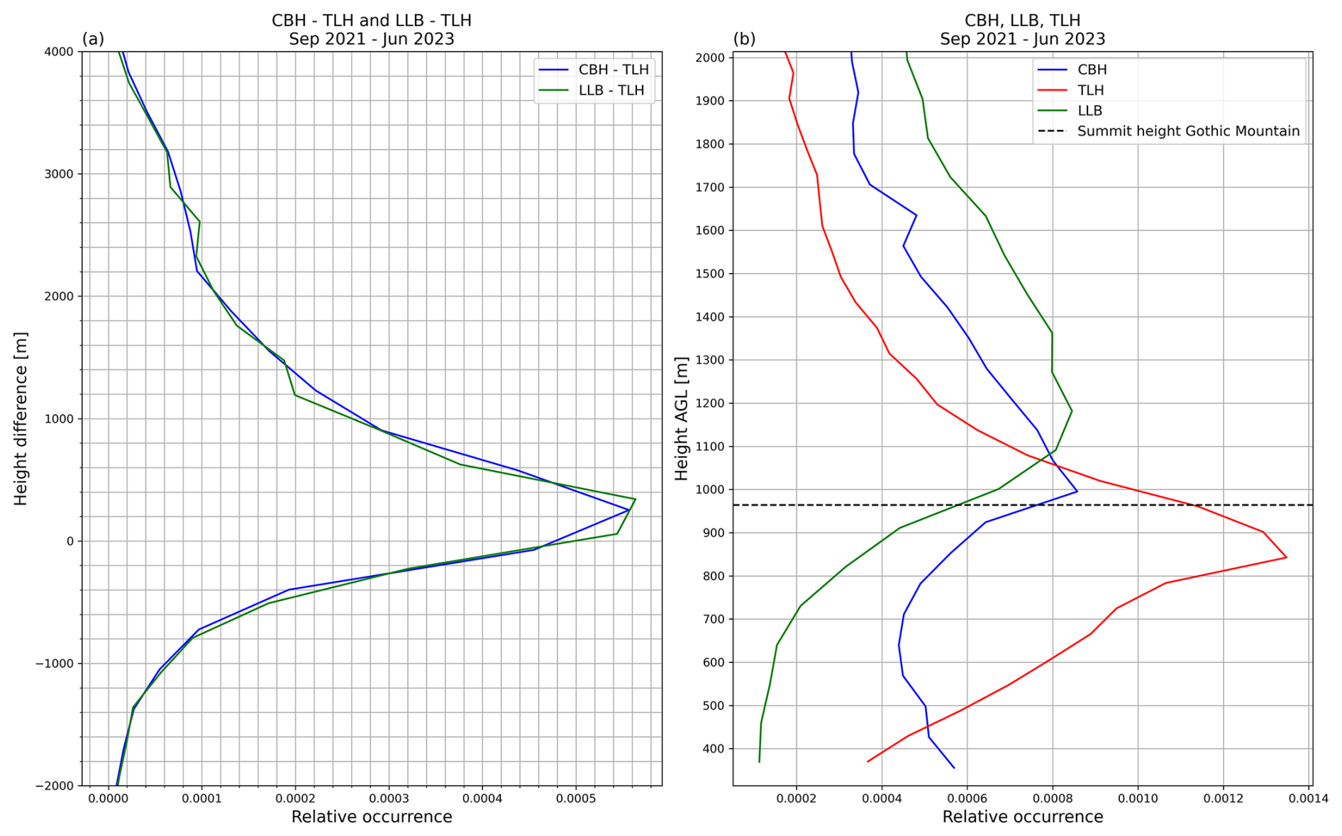
Figure 5 (a) Statistic of difference between CBH and TLH (blue line) and the difference between LLB and TLH (green line) for the duration of the SAIL campaign from September 2021 to end of May 2023. (b) Statistic of turbulent layer height detected as described in Sect. 2.6.1 (red line), ceilometer cloud base (blue line), liquid layer base height (green line) for the duration of the SAIL campaign from September 2021 to end of May 2023. The black dashed line marks the Gothic Mountain summit height.

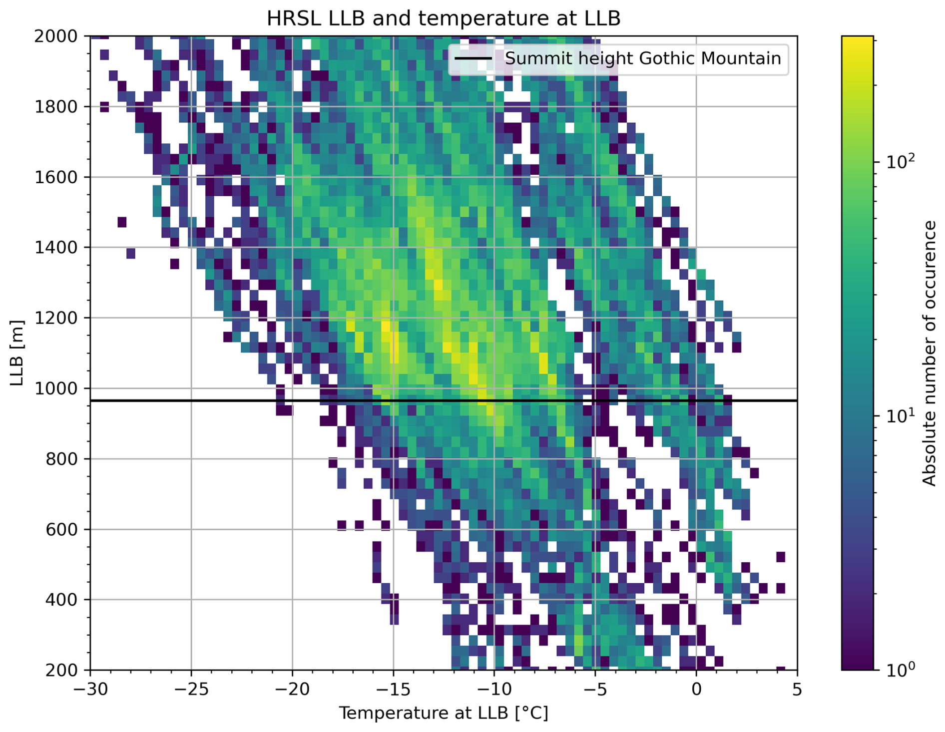
Figure 6 2D histogram of LLB height for the duration of the SAIL campaign from September 2021 to end of May 2023 derived from HRSL measurements, and the respective temperature at LLB height. The black solid line marks the Gothic Mountain summit height.

In Fig. 6 the HRSL LLB is plotted against the temperature at LLB height. The figure shows that cloud liquid is frequently found at heights between 900 and 1600 m a.g.l. with the maximum frequency of occurrence mostly in the vicinity of Gothic Mountain Summit and temperatures between −20 and −5 °C, theoretically allowing for riming even at temperatures down to −20 °C.

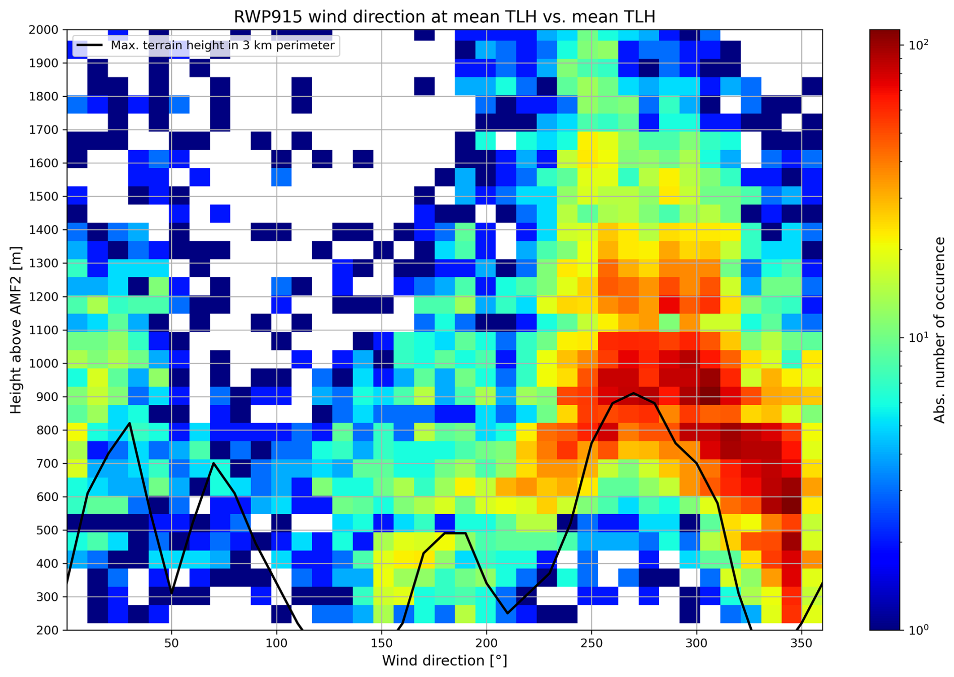
Figure 7 Absolute number of occurrence of TLH (retrieved as described in Sect. 2.6.1) plotted as a function of the wind direction at TLH (measured by the RWP915 between December 2022 and May 2023). The black line is the max. terrain height in a 3 km perimeter around AMF2 at the respective azimuth direction.

Due to the availability of the wind profiler RWP915 between December 2022 and May 2023, we can relate TLH to the wind direction in this period. It is important to notice that RWP915 data is only available during precipitation when hydrometeors serve as tracers for the wind direction. Wind during this time was strongly dominated by south, west and north wind, especially during significant precipitation events. The position of the measurement site in the East River valley introduces a complex terrain, strongly varying with azimuth direction (see Fig. B1 for a map of the local topography). To link the occurrence of turbulence to the surrounding orography we combined the TLH with the wind direction at TLH retrieved by RWP915 and the max. terrain height in a 3 km perimeter around the measurement site (see Fig. 7). The highest mountain close to the measurement site is Gothic Mountain, visible as a peak in orographic height between an azimuth of 240–310°. The occurrence of TLH closely resembles the shape of Gothic Mountain. At wind directions of 240–300°, the turbulent layer is located at summit height of Gothic Mountain or a few hundred meters above, likely forming along the edges of the counterflow behind Gothic Mountain as shown in Sect. 2.6. Slight changes in the wind direction to more southerly or northerly directions causes the TLH to decrease and the turbulence seems to be created along the flanks of Gothic Mountain. During southerly wind directions, a turbulent layer is created by Snodgrass Mountain which is a second, smaller summit south of the measurement site at an azimuth of 150–200°. During periods with northerly wind directions, the wind blows down the East River valley rather undisturbed and the turbulent layer appears anywhere between almost surface level and 1000 m a.g.l. Either the turbulence is formed along the flanks of Gothic Mountain and Avery Peak to the NE (0–50° azimuth), or the flow is still influenced by Mt. Bellview, a summit located 7 km to the NNW of Gothic. A turbulent layer is only rarely detected during wind directions between 50 and 150°, simply because these wind directions are uncommon during precipitation events in that region.

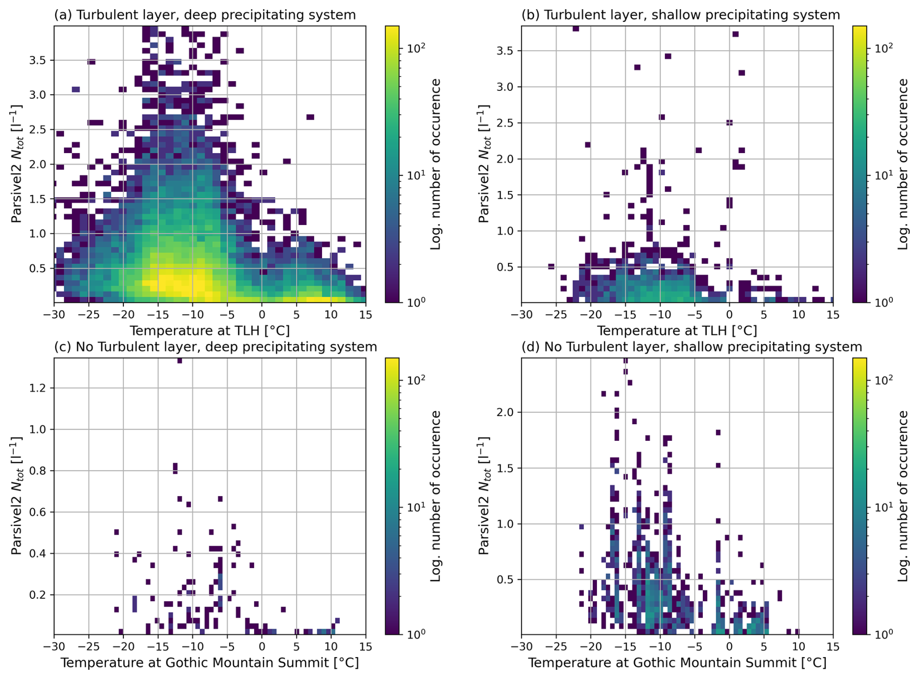
Figure 8 Temperature at TLH plotted as function of the Parsivel2 N_tot for different synoptic configurations. Data from September 2021 to June 2023 was analyzed. (a) A turbulent layer is present, KAZR Z_e between 500 m and 1.5 km above Gothic Mountain summit height exceeds −10 dBZ. (b) A turbulent layer is present, KAZR Z_e between 500 m and 1.5 km above Gothic Mountain summit height does not exceed −10 dBZ. (c) No turbulent layer is present, KAZR Z_e between 500 m and 1.5 km above Gothic Mountain summit height exceeds −10 dBZ. (d) No turbulent layer is present, KAZR Z_e between 500 m and 1.5 km above Gothic Mountain summit height does not exceed −10 dBZ.

Figure 8 shows temperature at TLH plotted against the total number of hydrometeors (N_tot) observed by the Parsivel2 at the surface for different synoptic configurations. Specifically, deep and shallow precipitating systems that either do or do not contain a turbulence layer are contrasted. If no turbulent layer was present, the temperature at Gothic Mountain summit height was used. Events where precipitation was detected without a turbulent layer are rare in the analyzed time span (panels c and d), highlighting the crucial role of turbulence in orographic precipitation, as it often accompanies precipitation, even if not directly causing it. The majority of precipitation events stem from deeper precipitation systems and a turbulent layer somewhere between −5 and −15 °C (panel a). The highest N_tot is also found in this temperature region. At temperatures between −10 and −20 °C, the turbulent layer is in an especially favorable temperature regime for precipitation formation via the WBF, as liquid water formed through updrafts can quickly transition into the ice phase. Furthermore, Takahashi et al. (1995) found that ice-ice collisions produce the highest number of splinters between −10 and −20 °C. The presence of SLW in this temperature region (see Fig. 6) may further enhance depositional growth and also riming, and SIP processes enhanced by turbulence may aid the formation of new particles, which we will discuss in detail in Sect. 3.2. Most interestingly, precipitation is also detected in the presence of a turbulent layer when only a shallow precipitating system is present. Such precipitation is most common at a temperature at TLH between −5 and −20 °C, but features much lower N_tot than deep precipitating systems. Precipitation originating from these shallow clouds may be entirely induced or at least augmented by orographic turbulence; however, definitive evidence remains elusive. Panel (d) for example shows that precipitation may fall from shallow precipitating systems without the presence of turbulence. We can provide some eye witness reports of these clouds, as during the installation of our instruments in Gothic, we had the chance to observe shallow precipitating clouds forming behind Gothic Mountain (see Fig. A1 in Appendix A).

3.2 Fingerprints of microphysical processes in the turbulent layer

In this section, we focus on the microphysical processes inside the turbulent layer and the fingerprints they leave in polarimetric cloud radar data. As mentioned, the problem is that radar observations inside the turbulent layer are masked by the turbulence itself (see Sect. 2.1.2). So instead of looking at radar data inside the turbulent layer, we compare radar variables above and below the turbulent layer and therefrom draw conclusions on microphysical processes inside the turbulent layer (Sect. 2.6.2). We specifically analyze four variables: KAZR Z_e, KAZR MDV, LIMRAD94 K_DP and LIMRAD94 $\mathrm{s}{Z}_{{\mathrm{DR}}_{\max }}$, in a period LIMRAD94 was measuring at constant elevation of 40° from December 2022 to February 2023. MDV is defined negative upward.

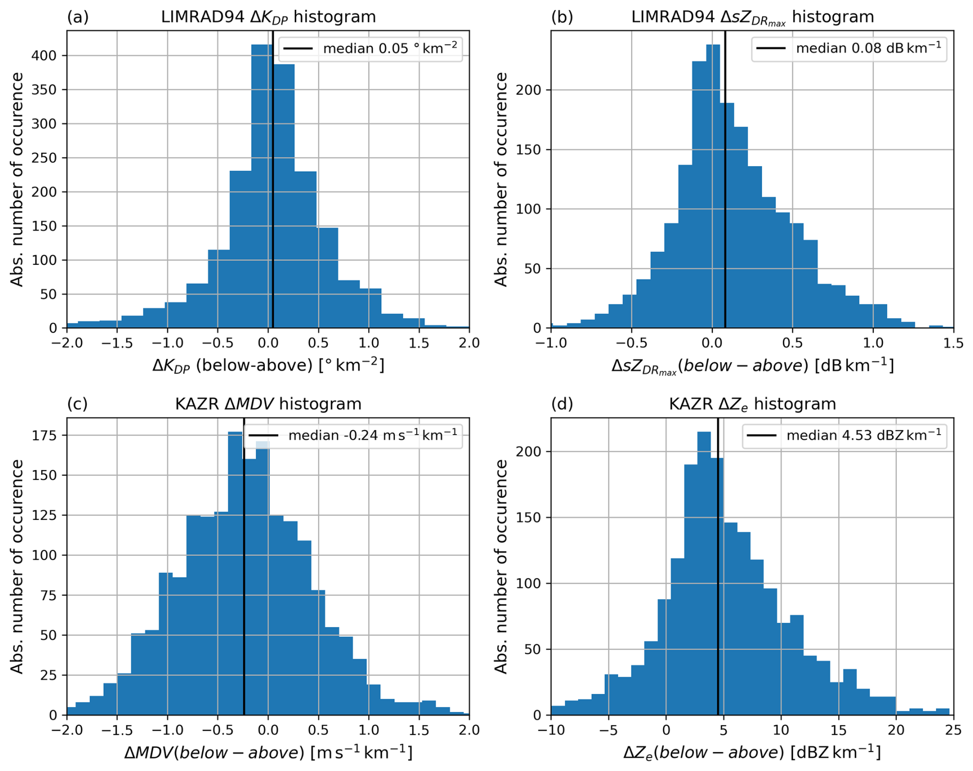
Figure 9 Histograms showing the difference of radar variables above-below the turbulent. (a) LIMRAD94 ΔK_DP, (b) $\mathrm{\Delta }\mathrm{s}{Z}_{{\mathrm{DR}}_{\max }}$, (c) ΔMDV, (d) KAZR ΔZ_e.

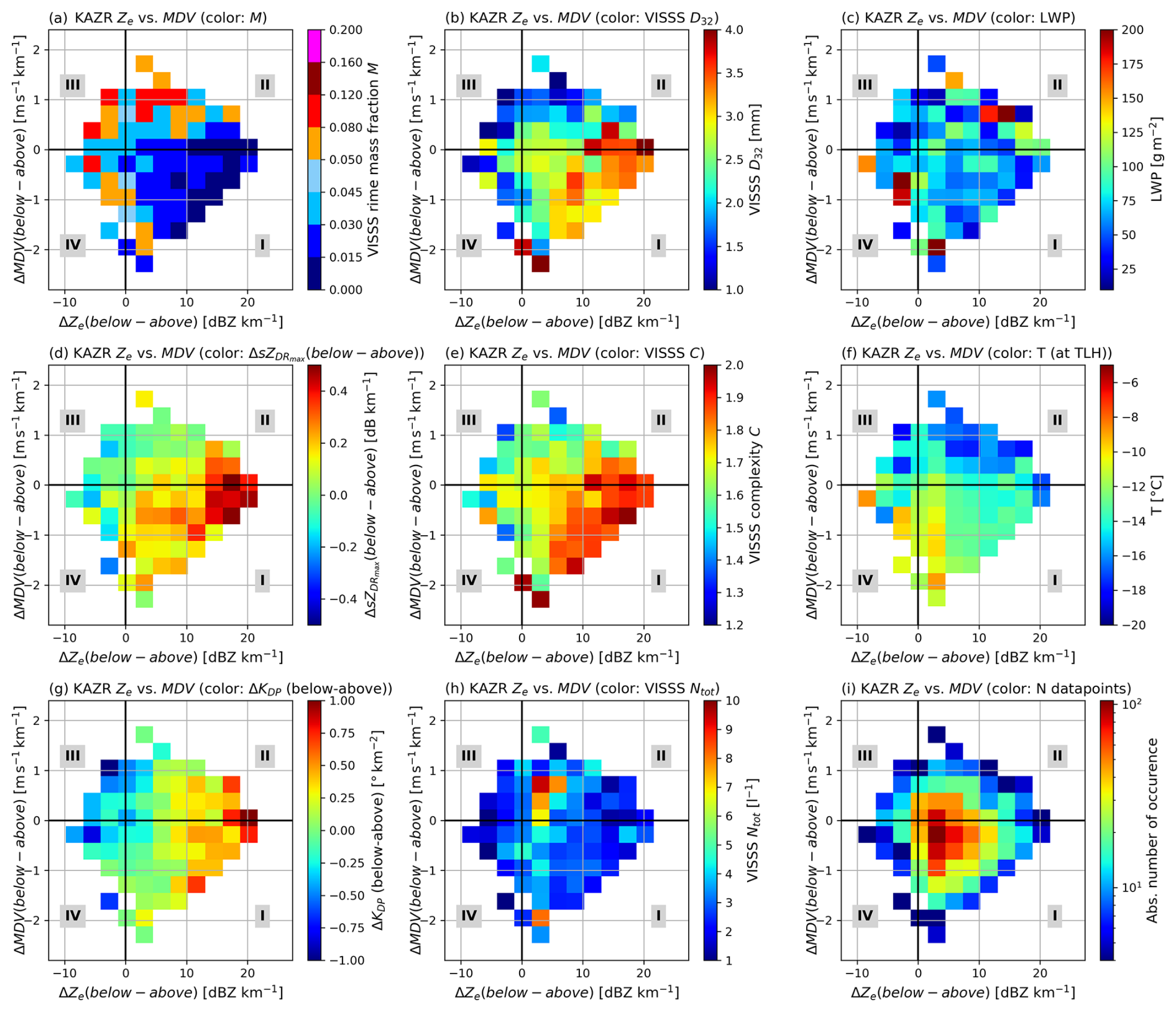
Figure 10 2D histograms showing the difference of radar variables below – above the turbulent layer, the color of each square represents the mean of a third variable. Each square contains at least 4 datapoints. MDV is defined negative upward. All panels divide the x-axis and y-axis into quadrants (I–IV). (a) KAZR ΔZ_e vs. ΔMDV, color: VISSS M, (b) KAZR ΔZ_e vs. ΔMDV, color: VISSS D₃₂, (c) KAZR ΔZ_e vs. ΔMDV, color: $\mathrm{\Delta }\mathrm{s}{Z}_{{\mathrm{DR}}_{\max }}$, (d) KAZR ΔZ_e vs. ΔMDV, color: VISSS C, (e) KAZR ΔZ_e vs. ΔMDV, color: LIMRAD94 ΔK_DP, (f) KAZR ΔZ_e vs. ΔMDV, color: VISSS N_tot

The histograms of the absolute change from above to below the turbulent layer are shown in Fig. 9. Negative/positive values indicate a decrease/increase of the respective variable within the turbulent layer, respectively. The change in K_DP (panel a) follows a near perfect Gaussian distribution centered around 0° km⁻¹. $\mathrm{s}{Z}_{{\mathrm{DR}}_{\max }}$ (panel b) reveals a tendency towards an increase below the turbulent layer, which gives a first hint on possible SIP mechanisms as $\mathrm{s}{Z}_{{\mathrm{DR}}_{\max }}$ increases when non-spherical ice particles are present. Below a turbulent layer, these ice particles might be splinters produced during ice collisional fragmentation. MDV (panel c) also shows a tendency to decrease below the turbulent layer, which means the particles velocity decreases inside the turbulent layer. This might be connected to the formation of a second, slower falling particle mode within the turbulent layer consisting of splinters, while the cases with increasing MDV point to the formation of rimed particles. Z_e (panel d) mostly increases inside the turbulent layer, which might be explained by increasing particle diameters inside the turbulent layer or also increased density (e.g. caused by riming) or increased number concentration of particles. It is apparent that we need to exploit the full polarimetric capacity of LIMRAD94 in combination with in-situ measurements by the VISSS to fully understand the microphysical processes inside the turbulent layer.

For that purpose, Fig. 10 illustrates a blend of various radar and VISSS variables, where radar variables are again represented as the difference between measurements above and below the turbulent layer. Surface-based VISSS variables assist in the classification of particle population characteristics. The plots are designed as 2D histograms between KAZR ΔMDV and ΔZ_e, while the color of each square represents the mean of a third variable that supplements the plot. Each panel domain is divided into four quadrants (Q) labeled I to IV. The absolute number of data points in each statistic is shown in panel (i).

Quadrant I

Quadrant I within each sub-panel comprises data points characterized by an increase in Z_e within the turbulent layer combined with a decrease in MDV (slower particle descent below the TLH compared to above it). This combination is the most common during the analyzed period as evidenced in panel (i), where the total number of data points is shown.

In panel (a), KAZR ΔMDV (below-above) is plotted against KAZR ΔZ_e (below-above) with the retrieved rime mass fraction M as color code. Quadrant I shows that an increase of Z_e in combination with a decrease of MDV (which means particles fall slower) below the turbulent layer can be attributed to mostly unrimed particles. A decrease in MDV which is accompanied by a Z_e increase of less than 5 dBZ km⁻¹ can generally be found in PSDs containing slightly rimed particles (light blue colors). In panel (b.I), the same radar variables are displayed together with VISSS D₃₂ as color. An increase in Z_e in combination with a decrease of MDV is mostly linked to a D₃₂ of 2.5 mm or higher. These situations are mostly found when also the mean complexity (panel e.I) is higher than 1.7. This points to the existence of aggregates, meaning the Z_e increase in these cases is caused by the increase in the particle diameter (Z_e∼D⁴, Moisseev et al., 2017) through aggregation in the turbulent layer. Towards the lower Z_e increase on the left of quadrant I, mean D₃₂ is mostly around 2.5 mm and also the complexity is slightly below 1.7. These ice particles appear to be slightly more rimed smaller aggregates that do not undergo major size increase inside the turbulent layer, which may indicate they are falling from aloft during deep precipitating systems. This is supported by the higher LWP visible in panel (c) on the left side of quadrant I. Temperatures towards the left of quadrant I are slightly higher (panel f), around or higher than −10 °C, indicating that this might be connected to deeper warm frontal precipitation.

Mean LWP in panel (c.I) ranges from under 50 g m⁻² in the outer edges to about 100 g m⁻² more towards the center and left of the plot. At the same time, the mean complexity (panel e.I) shows an inversely proportional behavior. This relation can be explained as follows: In deep frontal systems, especially along warm fronts, LWP might be increased which causes aggregates to be rimed, reducing their complexity. Contrarily, the lower the present LWP, the less riming can occur and hence the more complex the shapes of aggregates can be.

Panel (d.I) can be used to explain the decrease in particle fall velocity in combination with Z_e increase: the same combination of Z_e and MDV is combined here with $\mathrm{\Delta }\mathrm{s}{Z}_{{\mathrm{DR}}_{\max }}$ (below-above). The most significant increase in $\mathrm{\Delta }\mathrm{s}{Z}_{{\mathrm{DR}}_{\max }}$ (below-above) coincides with the strongest increase in Z_e and moderate decrease in particle fall velocity, but in the entire quadrant I, $\mathrm{s}{Z}_{{\mathrm{DR}}_{\max }}$ (below-above) generally tends to increase. Aggregates do not produce high Z_DR, therefore the increased $\mathrm{\Delta }\mathrm{s}{Z}_{{\mathrm{DR}}_{\max }}$ (below-above) points to a second particle mode of smaller, anisotropic ice at the slow edge of the Doppler spectrum which is formed inside the turbulent layer and causes the particle population as a whole (represented by MDV) to fall slower. A logical explanation would be the breakup of aggregates inside the turbulent layer through ice collisional fragmentation. This hypothesis is further supported by panel (g.I), where LIMRAD94 ΔK_DP was added as color. K_DP in quadrant I is mostly increasing inside the turbulent layer, which indicates a higher number of non-spherical particles, consistent with the hypothesis above. A small fraction of the K_DP increase might also be attributed to the presence of aggregates, as these can be responsible for up to 20 % of W-band K_DP (Kötsche et al., 2025). In the left section of quadrant I, K_DP typically exhibits minimal variation or might even slightly diminish within the turbulent layer. This is potentially due to negligible changes in particle concentration within the layer. The denser nature of rimed aggregates could reduce their likelihood of generating many splinters upon collision. As temperatures at TLH tend to be higher than −10 °C during this cases, the number of splinters per ice ice collision may further be reduced as shown in Takahashi et al. (1995). Particles rimed in the turbulent layer may also tend to become more spherical, resulting in a lower K_DP.

The temperature at TLH is shown in panel (f), for the pixels identified as containing mainly aggregates, it is very homogeneous between −12 and −15 °C. This appears to be a temperature where we see efficient aggregation inside the turbulent layer. As this is also still the temperature regime of the dendritic growth layer, it is reasonable to believe that splinters formed by ice collisional fragmentation quickly grow into dendrites and then aggregate as well. Enhanced supersaturation inside the turbulent layer might further aid new particle growth through deposition as also proposed by Lee et al. (2014) or Aikins et al. (2016). We analyzed radiosonde profiles measured during cases included in this statistic, almost all of them indicated supersaturation with respect to ice in the turbulent layer (not shown).

Panel (h.I) displays VISSS N_tot as color. N_tot ranges between 1 and 5 L⁻¹, which underlines that particle populations with many aggregates on average still contain a low number of particles because small, newly formed particles quickly aggregate as well. N_tot is slightly higher in the left of quadrant I, which combined with findings from the other panels, suggests deeper warm frontal precipitation with inherently higher N_tot.

The main suspected microphysical processes and their impact on VISSS and LIMRAD94 variables are shown in quadrant I of Fig. 11.

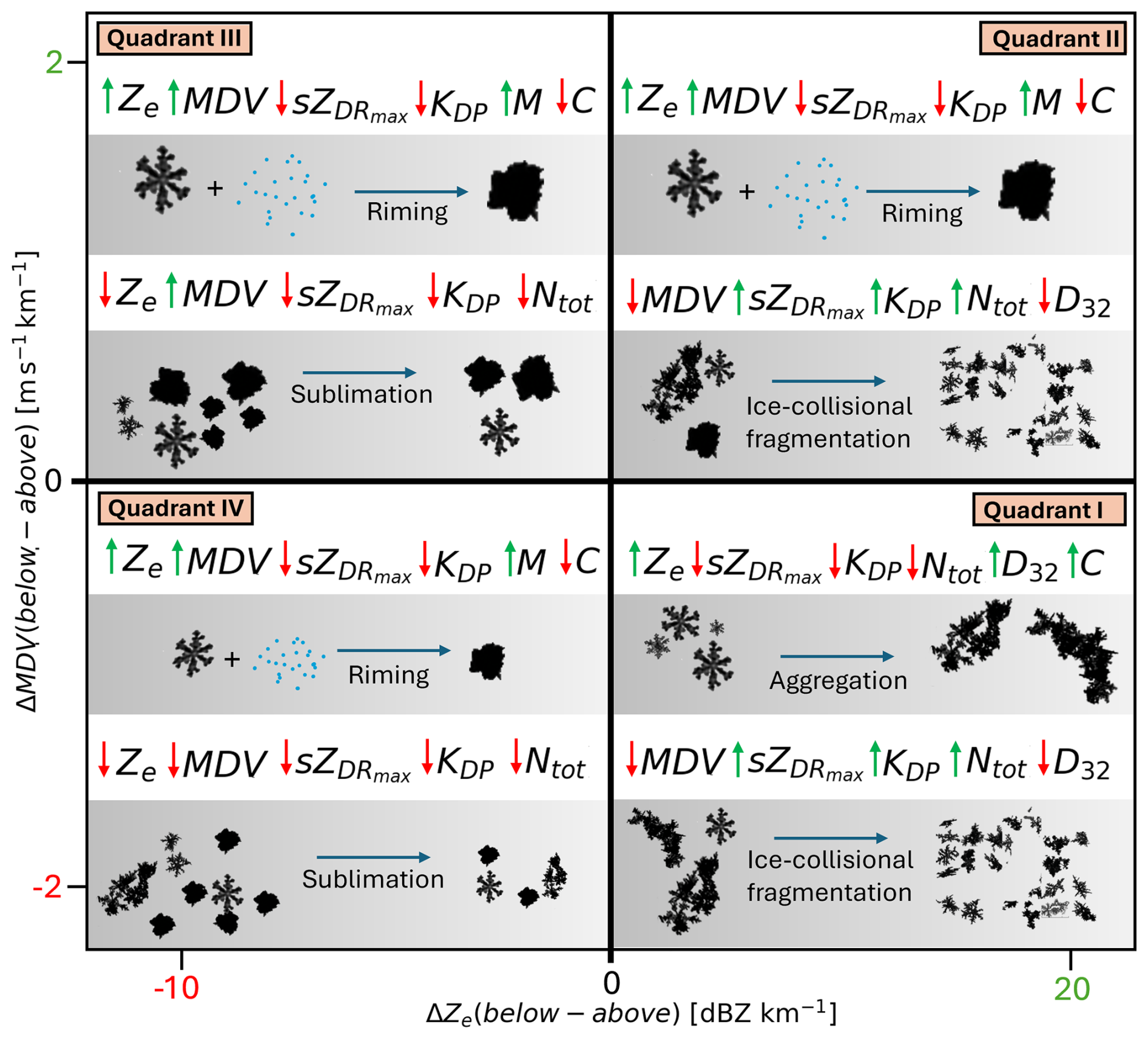
Figure 11 Conceptual diagram of the suspected (dominant) microphysical processes inside the turbulent layer, displayed similar to the four quadrants in Fig. 10. The impact of microphysical processes on radar and VISSS variables is also displayed qualitatively: Red downward facing arrows indicate a decrease of the respective variable, upward facing green arrows an increase. Note that for the radar variables (Z_e, MDV, $\mathrm{s}{Z}_{{\mathrm{DR}}_{\max }}$ and K_DP), we can measure the change inside the turbulent layer. VISSS variables (N_tot, C, D₃₂, M) are measured below the turbulent layer. Their change due to the microphysical process is suspected based on the change of particle and PSD properties. If a variable is not depicted, no clear trend can be derived. The shown particle images were recorded by VISSS.

Quadrant II

Quadrant II within each sub-panel comprises data points characterized by an increase in Z_e within the turbulent layer combined with a increase in MDV (corresponding to higher fall velocity of particles below the turbulent layer compared to above it). This combination is the second most common during the analyzed period as evidenced in panel (i).

In panel (a.II), increasing of Z_e in combination with a increase of MDV features more data points with higher M, these particles are rimed and fall faster due to the density increase, however, we also see pixels where near-zero M indicates unrimed particles, especially towards the highest Z_e increase. Looking at panel (b.II), particle populations generally feature lower D₃₂ values of 2.5 mm and smaller in some pixels to the left, but also higher D₃₂ especially to the right of quadrant II. The complexity in panel (e.II) depicts lower values of around 1.5 in some pixels. Still, we also see many pixels with higher complexities indicating both more rimed aggregates and graupel, but also PSD mainly inheriting unrimed aggregates.

Panel (d.II), compared to quadrant I, generally indicates a smaller increase in $\mathrm{s}{Z}_{{\mathrm{DR}}_{\max }}$ (below-above) inside the turbulent layer or even a slight decrease, especially for pixels with higher M. As Z_DR is closely connected to the particle shape, this decrease may be caused by riming as it tends to render small particles more spherical. For the same reason, K_DP in the left half of panel (g.II) displays little change or slight decrease inside the turbulent layer for more rimed PSDs. Pixels in the right part of II indicate an increase of $\mathrm{s}{Z}_{{\mathrm{DR}}_{\max }}$ (below-above) and K_DP, cross checking with the other panels, these are also pixels where D₃₂ is enhanced and M is low, which are likely particle populations consisting of aggregates producing splinters via ice collisional fragmentation as in quadrant I. We may also see PSDs with coexisting aggregates and graupel particles which we described in Kötsche et al. (2025). The turbulent layer may produce pockets of SLW, causing some particles to be heavily rimed while others experience less riming (e.g. Medina and Houze, 2015). This can lead to more efficient ice collisional fragmentation through greater differences in fall velocity and density. These collisions were found to produce up to 500 fragments per collision by Grzegorczyk et al. (2023). They also showed that the number of splinters increased with increasing collision kinetic energy, which depends on both the particle masses and the square of their relative velocity. In panel (f.II), it is noteworthy that for many pixels with high M, temperature at TLH is below −15 °C, although the overall number of datapoints is low (see panel i). This result differs from previous studies like Kneifel and Moisseev (2020) who found that riming is very uncommon at temperatures colder than −10 °C. The reason is likely that they did not analyze sites influenced by orographic turbulence like in this study. As we did show in Fig. 6, SLW close to Gothic Mountain Summit can be found at temperatures down to −20 °C (see Fig. 6). This implies the turbulent layer is producing SLW even at temperatures way below −10 °C and hence enables riming.

In panel (h.II), VISSS N_tot interestingly shows very high values for the pixels with high M and low D₃₂, indicating high number concentration of small graupel particles. This is consistent to the findings of Lee et al. (2014) who showed that turbulence can lead to a relatively large number of small-sized graupel particles.

See Fig. 11, quadrant II for a schematic view of the main microphysical processes described above.

Quadrant III

Panel (a.III) inherits a combination of decreasing Z_e and increasing MDV (meaning that the particles below the turbulent layer inherit higher fall velocity compared to the ones above it). This combination appears quite infrequently (see panel i.III) and seems physically atypical, as an increase in particle fall velocity usually indicates a size and/or density increase. The reduction in Z_e is up to −10 dB km⁻¹. Quadrant III features mostly rimed particle populations (panel a) and variable D₃₂ between 1 and 3 mm, while pixels with below 2 mm prevail (panel b.III). $\mathrm{s}{Z}_{{\mathrm{DR}}_{\max }}$ and K_DP both show decreasing tendencies in the turbulent layer (panels d.III and g.III), which indicates that small, non-spherical particles are depleted, a signal which may be attributed to sublimation. VISSS N_tot in panel (h.III) agrees with that hypothesis, as the particle populations mostly contain less than 2 L⁻¹. As the small particles in the PSD vanish, MDV will indicate faster falling particles because now the remaining larger particles dominate the spectrum. Given the very low number concentrations, spatial inhomogeneity may also be a reason for the observed behavior of Z_e and MDV.

Quadrant IV

Panel (a.IV) inherits a combination of decreasing Z_e and decreasing MDV (meaning particles below the turbulent layer fall slower than above it), such situations were rarely observed (panel i). Counterintuitively, we see a rather high fraction of more rimed PSDs (higher M). D₃₂ ranges between 1.5 and 3 mm. The complexity also differs between the pixels (panel e.IV), indicating a mix of graupel and less rimed particles. For pixels with high D₃₂, the complexity is also high, indicating some aggregates. $\mathrm{s}{Z}_{{\mathrm{DR}}_{\max }}$ and K_DP both exhibit a slight decreasing or indifferent tendency, which corroborates the depletion of small particles. Nevertheless, it is plausible that both metrics were initially close to zero, as small, rimed particles with low N_tot are unlikely to generate pronounced signals in K_DP or Z_DR. VISSS N_tot in panel (h.III) indicates low number concentrations of below 2 L⁻¹. Combined, these signatures points to sublimating particles in different stages of riming. As these particles sublimate, they lose mass causing them to fall slower. Without the presence of faster falling particles in the PSD, this may cause a decrease in fall velocity across the whole PSD. As for quadrant III, spatial inhomogeneity may also be a reason for the observed behavior of Z_e and MDV.

4 Summmary and conclusions

In this study, we conducted a long-term observational study during the SAIL campaign in Gothic, Colorado. We used a unique and closely collocated instrument setup combining a slanted polarimetric W-band radar (LIMRAD94), a vertically pointing ARM Ka-band radar (KAZR), the Video In Situ Snowfall Sensor (VISSS) and a high resolution spectral lidar (HRSL) as well as other instruments to investigate the characteristics of orographic turbulent layers based on long-term statistical analysis (Sect. 3.1). To draw conclusions on cloud microphysical processes inside the turbulent layer, we analysed the data of LIMRAD94 and KAZR data using a novel method to assess microphysical processes by comparing radar variables above and below the turbulent layer, avoiding direct in-layer radar signal degradation from turbulence (Sect. 3.2). These results are shown in Figs. 9 and 10.

To conclude our study, we would like to highlight the following key findings:

• A turbulent layer was almost always present at the site in Gothic during precipitation events between September 2021 and May 2023. The temperature at TLH during these events was mostly between −5 and −20 °C – a favorable region for aggregation, riming, and secondary ice production (SIP). Precipitation from shallow clouds in connection with a turbulent layer was also frequently seen in this statistical analysis, which underlines the importance of orographic turbulence for precipitation formation (Fig. 8).

• Aggregation is a dominant process inside the turbulent layer and frequently occurs at temperatures between −12 and −15 °C (temperature at turbulent layer height). It is responsible for Z_e increase of up to 20 dBZ km⁻¹ and reduction of the mean particle fall velocity. This reduction is connected to the formation of small, anisotropic particles through SIP. This theory is supported by increasing $\mathrm{s}{Z}_{{\mathrm{DR}}_{\max }}$ and increased K_DP inside the turbulent layer in connection to the aggregation signals (Fig. 10). This indicates SIP through ice-collisional fragmentation producing new, anisotropic ice splinters that may quickly grow into dendrites, given the favorable temperature regime for depositional growth. These results are consistent with the conclusions presented in Chellini and Kneifel (2024).

• Riming frequently occurs inside the turbulent layer, Z_e may increase by up to 15 dBZ km⁻¹ while particle fall speeds always increase. Changes in K_DP or $\mathrm{s}{Z}_{{\mathrm{DR}}_{\max }}$ during riming cases with high rime mass fraction M are mostly minor with a slight decreasing tendency, likely due to particles becoming more spherical. We frequently detected riming where the temperature at turbulent layer height (TLH) was below −15 °C. This implies the turbulent layer is producing SLW even at temperatures way below −10 °C and hence enables riming, contrary to the findings of Chellini and Kneifel (2024) who found riming mainly at temperatures warmer than −10 °C.

• We observe sublimation below the turbulent layer. This is characterized by a decrease in Z_e, K_DP and $\mathrm{s}{Z}_{{\mathrm{DR}}_{\max }}$ in combination with an increase or decrease in MDV. Often, these sublimation cases feature enhanced M. We speculate that small graupel may be forming in a shallow cloud layer inside the turbulent layer and sublimates in the well mixed boundary layer. Sublimation in connection to turbulence was also reported by e.g. Lee et al. (2014) and Ramelli et al. (2021).

• Statistical analysis showed that TLH is strongly tied to the surrounding terrain and the wind direction at turbulent layer height (see Fig. 7). TLH is often collocated with the cloud base height and supercooled liquid water layers near the summit height of Gothic Mountain (Fig. 5). This implies the turbulent layer is producing SLW which was also found by many other studies in the past (e.g. Houze and Medina, 2005; Houze, 2012; Medina and Houze, 2015; Ramelli et al., 2021, among others). The frequent collocation of cloud base height and TLH may be further explained by mechanical mixing of the boundary layer due to turbulence and increased moisture convergence in the lee of Gothic Mountain.

The authors note that the measurement location has intricate terrain and unique synoptic forcing mechanisms. Therefore, the findings are particular to this specific environmental and synoptic scenario and may not be applicable to different locations or situations. Nevertheless, the presence of analogous mountainous and valley structures throughout the Rocky Mountains suggests that comparable processes are likely to occur, which may result in notable congruence with our findings. We particularly highlight a recent campaign named S2noCliME (Pettersen et al., 2024) in the Rocky Mountains. A wide facet of instruments including multiple radar frequencies was deployed in the Park Range of Northwest Colorado during the 2024–2025 winter season. The data gathered there may provide further insights into the microphysical processes connected to orographic turbulence and we strongly recommend exploiting the data set with this special focus on orographic turbulence.

Our findings highlight the importance of orographic turbulence in precipitation enhancement, even in shallow clouds or without the presence of deep precipitating systems. This topic should be addressed in future studies. We demonstrated how radar polarimetry may be used to investigate microphysical processes inside a turbulent layer avoiding the dampening effects of turbulence on radar polarimetry.

Appendix A: On site images of cloud formation behind Gothic Mountain

Figure A1 shows a precipitating cloud forming behind Gothic Mountain, we observed these clouds very frequently on site during the installation of our instruments.

Figure A1 Image of a precipitating cloud behind Gothic Mountain on 22 October 2022 at 16:42 UTC. Courtesy: Anton Kötsche.

Appendix B: Map showing the local topography

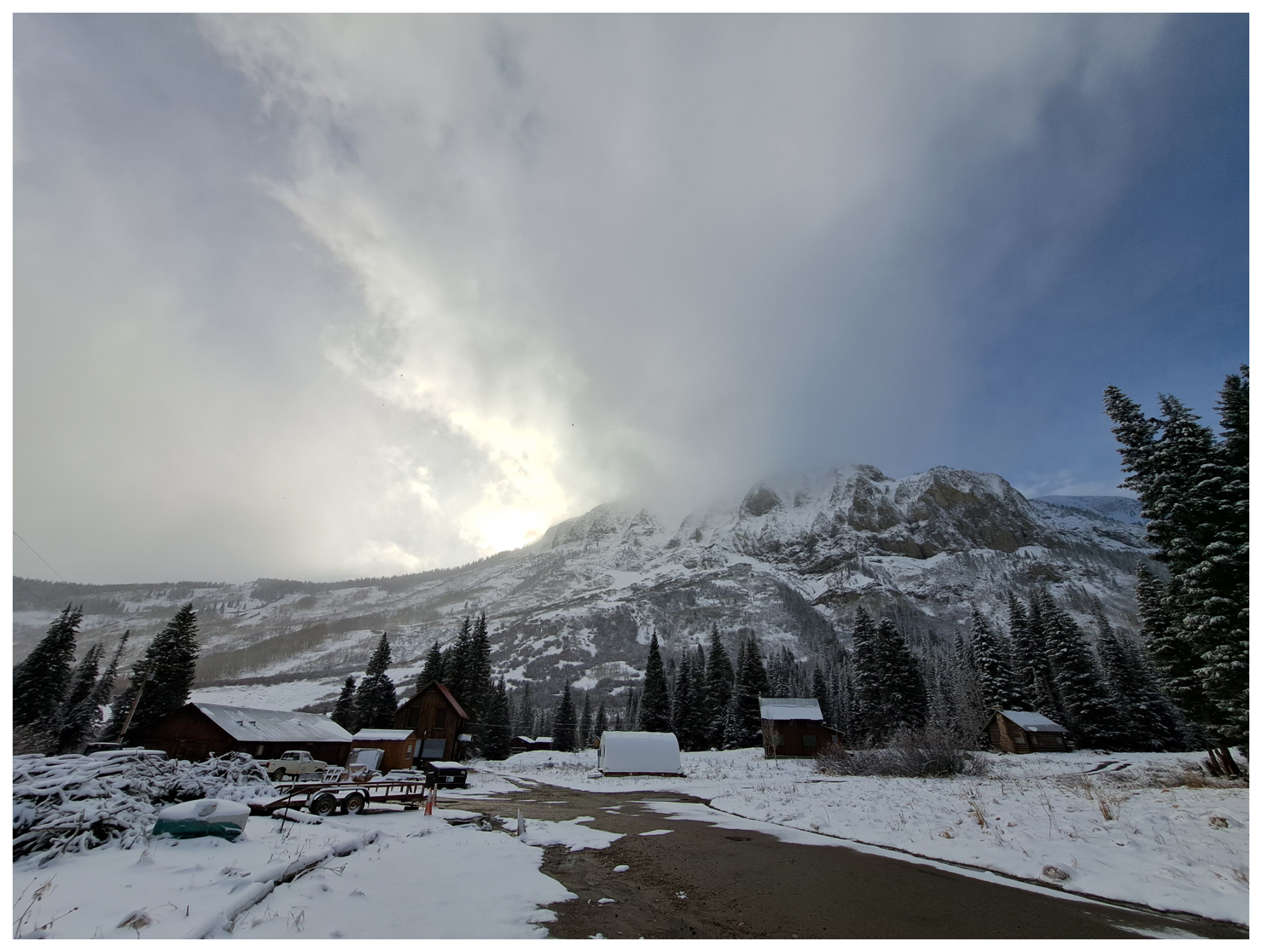
Figure B1 shows the local topography around the measurement site with all relevant mountain peaks and instrument locations marked.

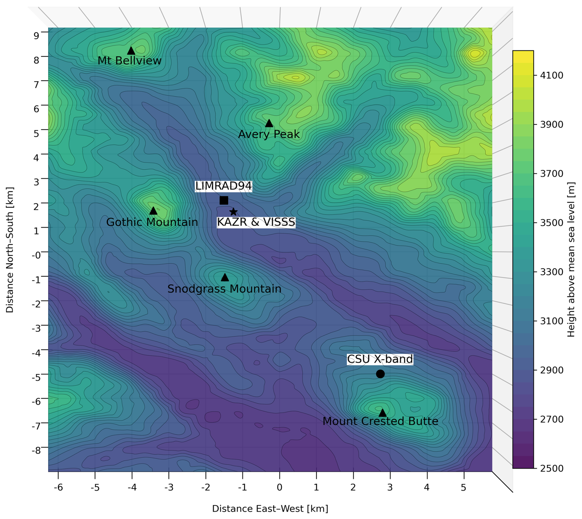
Figure B1 Elevation showing the local topography around the measurement site with all relevant mountain peaks and instrument locations marked. In this view, north corresponds to the top edge of the plot, and east corresponds to the right edge; south and west follow accordingly. Blue and yellow colors mark low and high elevation, respectively.