Advancements and continued challenges in observations and global modelling of atmospheric ice mass

We assess the current status of atmospheric ice mass estimates by first critically comparing satellite-based datasets, then examining global circulation and global storm-resolving models. The analysis focuses on the frozen water path, which offers a more consistent measure across modelling and observational datasets than cloud ice or other partial quantities. As a reference, we use three retrievals derived from the CloudSat mission. Despite using the same input data, these retrievals exhibit a significant spread. Still, common biases cannot be ruled out, and we argue that the uncertainty in overall means can be as high as 30 %. A recently developed machine learning product based on passive thermal infrared observations greatly extends the spatial and temporal coverage available for comparisons, but its local precision is limited compared to radar-based retrievals.

Global circulation models continue to underestimate frozen water paths compared to the observational benchmark and fail to provide consistent representations of regional temporal changes or the annual cycle. Storm-resolving models, which operate at finer grid spacing and explicitly resolve convective dynamics, show better representation of total ice mass, with variations among them similar to the observational uncertainty. However, several issues were noted, such as apparent deviations in the spatial structures of tropical deep convection, and they differ significantly in their relative amounts of cloud ice, snow, and graupel. Together, these findings reveal progress but highlight continuing uncertainties that limit confidence in projections of cloud-related climate feedbacks.

1 Introduction

In a broad review, Waliser et al. (2009) found that the status of cloud ice modelling was unsatisfactory, but there were expectations of progress. As a basic illustration of the shortcomings of the time, a number of global circulation models (GCMs) were shown to vary by a factor of 20 in their reported global mean cloud ice mass. On the other hand, there was hope for progress as more advanced treatments of atmospheric ice were being introduced in GCMs, and new satellite sensors were about to provide better observational constraints. Here, we investigate if the expected improvements have been realised by exploring the status of atmospheric ice mass in present sets of global models and satellite datasets.

A discussion of atmospheric ice must begin by clarifying terminology. Already the term “cloud ice” is a source of confusion. Inside atmospheric models, cloud ice is normally limited to the fraction of ice particles having a low terminal sedimentation velocity, and can be denoted as “suspended”. However, there is no general agreement on a threshold value setting an upper limit in terms of particle fall velocity or size. The remaining ice particles, of larger dimension, are classified as either snow (low density and medium fall speed) or graupel (high density and fall speed). It is noteworthy that the data request document for the latest Coupled Model Intercomparison Project (CMIP6) in effect defines cloud ice as the ice categories considered by the model's radiation scheme (CMIP6 Data Request, 2026). As a consequence, there is still no strict definition of cloud ice found in GCM output.

The vague definition of “cloud ice” was stressed by Waliser et al. (2009) and it was acknowledged that the high deviation between GCMs could partly be attributed to this issue. That is, an equal comparison was not possible and the actual status could not be established.

Compared to cloud ice, a more clear target for a comparison would be to assess the total ice mass. However, this option is of limited applicability for GCMs. This is the case as all, or a large fraction, of the precipitating ice is simply not represented in their output. Accordingly, atmospheric ice masses in GCMs remain difficult to characterise, but the situation is different for the emerging class of global storm resolving models (GSRMs, i.e. models having a horizontal grid spacing in the order of 5 km). Compared to the high degree of parametrisation applied in GCMs, some processes have, to a larger extent, a direct physical representation in GSRMs (Satoh et al., 2008). Clouds are explicitly resolved and the mass of all ice hydrometeor categories are in general prognostic variables.

As also pointed out by Waliser et al. (2009), as well as by Eliasson et al. (2011, 2013), there are similar considerations when approaching datasets of satellite-based estimates of atmospheric ice mass. One aspect is the sensitivity of the measurement to the particle size distribution (PSD). The rule of thumb is that a remote measurement is most influenced by particles whose sizes are of the same magnitude as the wavelength observed; the measured signal at optical and infrared wavelengths will mainly be governed by the smallest particles, while at microwave wavelengths the larger end of the PSD will dominate the impact.

As an example, the satellite-based cloud radars launched so far, the Cloud Profiling Radar (CPR) onboard CloudSat and the CPR onboard EarthCARE (Earth Cloud, Aerosol, and Radiation Explorer), operate at a wavelength of about 3 mm (94 GHz). In many situations, this wavelength is considerably larger than all the ice hydrometeors in the probed air volume. In this case, the back-scattering is proportional to D⁶ (Rayleigh conditions), where D is particle size. The strong dependency on size implies that the measured reflectivity will mainly be generated by the largest particles, despite likely being relatively few; the large particles outshine the small. As a result, additional information is needed to estimate the mass of the non-sensed particle fraction, to map the observed reflectivity to an estimate of the total ice mass.

The same overall logic applies to passive observations: the measurement provides relatively direct information on a fraction of the ice particles. However, the exact size range probed is case-specific, depending on the shape of the local PSD, and no instrument nor retrieval setup is yet capable of isolating e.g. the suspended cloud ice mass. As for models, presently the only clear target for estimates of atmospheric ice contents is the total mass.

Satellite observations are not only limited in terms of particle size, but also with respect to distance into the cloud systems (Eliasson et al., 2011). For active systems (lidars and radars), the emitted signal can be attenuated before reaching the ground level, and for passive systems the optical depth can be too high to effectively probe lower levels. Here, optical and infrared are at an even greater disadvantage, as the attenuation caused by ice crystals increases when decreasing the wavelength, due to the shift towards the impact of smaller (but more numerous) particles discussed above. For the satellite-based cloud radars, strong attenuation is a limitation only for most dense cloud systems. On the other hand, they are affected by surface clutter and there is a blind zone present throughout, extending about 1 km above the surface.

It is also noteworthy that the nomenclature differs between the model and observation communities, for example, in the meanings of ice water content (IWC) and its column counterpart, ice water path (IWP). These terms are commonly used to name retrieval results and, at least in some satellite datasets, refer to the total ice mass. However, if used in conjunction with atmospheric models, IWC and IWP refer only to the cloud ice fraction. To avoid confusion inside this work, the total of all atmospheric ice is denoted as the frozen water. That is, the frozen water content (FWC) is the sum of the ice, snow, and graupel water contents (shortened as IWC, SWC, and GWC, respectively). Some authors have used the term “total ice” (TIWC) as an alternative to frozen water. The vertical integral of FWC will be denoted as the frozen water path (FWP). When averaged, FWP and other ice mass variables throughout refer to “all-weather” means (and not to “in-cloud” means, another averaging strategy).

The aim of this work is to assess the current agreement between satellite retrievals and global models, both within and across the two data sources. We focus the comparisons on FWP for several reasons. FWP is directly proportional to the latent heat released during the conversion of water vapour to ice, and is thus involved in the coupling between clouds and atmospheric circulation (Bony et al., 2015). It can be used to estimate precipitation efficiencies, the fraction of hydrometeor condensation that ends up as surface precipitation (Kukulies et al., 2024b), as well as for tracking convective storms (Kukulies et al., 2024a). The impact on longwave radiation at the top of the atmosphere is, on average, rather proportional to the logarithm of FWP (Deutloff et al., 2025), and not the mean FWP (Berry and Mace, 2014).

Further, there are now global models (GSRMs) reporting the mass of all ice hydrometeor types and the arguably most reliable satellite retrievals, 2C-ICE and DARDAR (Sect. 2.1), estimate this total mass. In any case, total ice is, so far, the only mass quantity consistently defined across models and observations. DARDAR (raDAR/liDAR) and 2C-ICE have been used as the reference in many studies, but are frequently used separately (e.g. Lee and Wing, 2024; Vérèmes et al., 2019; Bjordal et al., 2020; Nugent et al., 2022). Here, both these datasets are considered and confronted to show that they deviate significantly despite using the same measurement input. Besides mean FWPs, the assessment of GSRMs considers the representation of tropical deep convection in terms of organization and diurnal cycles. DARDAR and 2C-ICE do not offer sufficient coverage for addressing these questions and a dataset representing the state of the art for passive retrievals is also applied (Chalmers Cloud Ice Climatology, Sect. 2.1). As described above, for GCMs having fewer hydrometeor output variables and coarser resolution compared to GSRMs, we are so far limited to considering cloud ice, but we still provide a comparison between the models that participated in CMIP6 to establish a link with earlier similar studies.

The following section introduces the datasets used. Section 3 critically compares satellite retrievals of FWP to elucidate their limitations and to establish a reference for the assessment of GCM and GSRM models, found in Sects. 4 and 5, respectively.

2 Data

2.1 Satellite retrievals

2.1.1 Background

Considering how electromagnetic radiation interacts with ice hydrometeors and the spatial resolution achieved by passive and active instruments, estimates of FWP based on cloud radar reflectivities must be considered the most reliable. CloudSat's CPR became the first space-based cloud radar when it was launched in 2006 (Stephens et al., 2008). Multiple retrievals exist involving CloudSat, where 2C-ICE (Deng et al., 2010, 2015) and DARDAR (Delanoë et al., 2014; Cazenave et al., 2019) are two widely used ones. In-depth comparisons of 2C-ICE and DARDAR are relatively few; exceptions include Heymsfield et al. (2008); Deng et al. (2013, 2015); Winker et al. (2024), and several recent papers highlight deviations in the occurrence fractions of FWP from DARDAR and 2C-ICE, as well as substantial differences between DARDAR versions 2 and 3 (Atlas et al., 2024; Sokol et al., 2024; Gasparini et al., 2025).

Retrievals based on passive measurements tend to give considerably lower column ice mass values. This can largely be understood by the fact that 2C-ICE and DARDAR provide estimates of the total ice hydrometeor mass, while the passive datasets tend to only reflect parts of the ice column. Sensors recording optical and infrared radiation are most sensitive to the cloud top layer, with, as mentioned, the signal dominated by small ice crystals. As a consequence, retrieved values have often been interpreted as estimates of the cloud ice mass, roughly corresponding to the suspended fraction of ice particles. Microwave radiation propagates relatively unimpeded through ice clouds and the interaction is dominated by the largest ice particles. This is also the situation for cloud radars, but a higher FWP is required for obtaining a measurable signal with a microwave radiometer. As traditional passive retrievals have been shown to have a strong bias with respect to CloudSat-based ones (e.g. Eliasson et al., 2011; Duncan and Eriksson, 2018), they are excluded from this study.

A new manner to extract FWP from passive observations is to apply machine learning, using a CloudSat dataset as the reference. An early example on such retrievals was SPARE-ICE (Synergistic Passive Atmospheric Retrieval Experiment-ICE; Holl et al., 2014), that Duncan and Eriksson (2018) found to agree well with DARDAR in the tropics but to still exhibit a low bias at mid-latitudes. However, SPARE-ICE was only produced for a limited time period. A newer machine learning-based product is CCIC (Chalmers Cloud Ice Climatology, Amell et al., 2024). By making use of homogenised datasets of geostationary data, quasi-global coverage over decades at high spatial resolution is achieved. As cloud radar data only cover a limited time period, have very low instantaneous spatial coverage and are limited in diurnal sampling (as flown in sun-synchronous orbits), a dataset like CCIC emerges as a potentially very important complement.

2.1.2 Included active datasets

CloudSat was launched in 2006 into a sun-synchronous orbit and initially provided observations during both day and night, at around 01:45 LST. Due to a battery failure, occurring in 2011, the measurements were limited to the day passage for the later part of the mission until the instrument was turned off in 2023. The horizontal and vertical resolutions of measured reflectivities are about 1.5 and 0.5 km, respectively.

Three retrievals involving the CloudSat CPR radar are considered and compared. The first two, 2C-ICE and DARDAR, apply the optimal estimation method (OEM, Rodgers, 2000). Both also take input from the CALIOP (Cloud-Aerosol Lidar with Orthogonal Polarization) lidar onboard CALIPSO (Cloud-Aerosol Lidar and Infrared Pathfinder Satellite Observations) that flew in tandem with CloudSat. Here we give less attention to the lidar side as it is judged to have a small impact on the overall mean FWP, in comparison to the radar input. As a complement to these established datasets, radar-only retrievals using an algorithm of “onion peeling” character were also made. Although both DARDAR and 2C-ICE use OEM, the implementations are not the same with the most critical differences being assumptions regarding microphysics.

DARDAR version 3.1 (Cazenave et al., 2019) is selected for this study. It is not possible to discern liquid and ice particles from CloudSat CPR reflectivities alone. In the DARDAR algorithm, all reflectivities measured at temperatures below 0 °C are assigned to the ice phase. Cloud liquid droplets are too small to generate significant back-scattering at 94 GHz, but the DARDAR approach still assumes that there exist no super-cooled liquid droplets with a size matching drizzle or stronger rain. The ice hydrometeor particle model combines the oblate spheroid representation from Hogan et al. (2012) and the particle size distribution (PSD) from Delanoë et al. (2014) with updated mass-size relation parameters and the calculation of scattering properties assuming totally randomly oriented particles (Cazenave et al., 2019). Only molecular absorption is considered for two-way attenuation of the radar signal.

The 2C-ICE version included is R05. To distinguish ice from liquid in 2C-ICE, cloud phase from the 2B-CLDCLASS-LIDAR (Sassen et al., 2008) product is used. 2B-CLDCLASS-LIDAR locates the presence of liquid water by identifying a sharp increase in the lidar signal followed by a sharp decrease, arising first from lidar's high sensitivity to cloud water and then strong attenuation. If water is present, 2B-CLDCLASS-LIDAR product defines the layer as mixed phase if the cloud layer top is colder than −7 °C and the maximum radar backscatter exceeds a temperature-dependent threshold. If 2B-CLDCLASS-LIDAR classifies the region as pure ice, 2C-ICE performs a retrieval. If the layer is classed as mixed phase, 2C-ICE performs retrievals of ice mass from measurements at temperatures below −4 °C. As for DARDAR, ice hydrometeors are treated to be totally randomly oriented (Deng et al., 2010), but a mix of particle habits following Baum et al. (2005) is assumed with single scattering properties taken from Hong (2007). Attenuation due to both molecular absorption and ice hydrometeors is accounted for.

As a complement and as a way to test the impact of different assumptions, a module from the Atmospheric Radiative Transfer Simulator (ARTS, Buehler et al., 2025) was applied. These inversions start at the radar range gates with the highest altitude, where a unit transmission can be assumed. The inversion continues downwards, one height range at a time, using the integrated extinction through the higher ranges to estimate the unattenuated reflectivity from the measured one. Retrieving one layer at a time in this fashion has been denoted as “onion peeling” (Rodgers, 2000). We adopt this term and denote the approach as ARTS onion peeling (AOP). In this work, the nominal setup of ARTS assumes that all back-scattering below 0 °C is due to ice particles (like DARDAR). Ice hydrometeors are represented as a particle model consisting of a large plate aggregate habit, taken from the ARTS single-scattering database (Eriksson et al., 2018), and the PSD of Field et al. (2007). The attenuation correction considers extinction by molecules and ice hydrometeors. Further details of AOP are found in Appendix A.

It is noteworthy that the PSDs of DARDAR and 2C-ICE both have two free parameters at each altitude, while in the radar-only regime (i.e. below the penetration depth of the lidar) there is only one piece of information per height range coming from the measurement. For this reason, a considerable vertical correlation is assumed for one of the two free parameters, to stabilize the retrieval. The AOP takes another approach, using PSDs that have a single free parameter. As a consequence, for two reflectivities, measured at the same temperature, AOP gives the same FWC in both cases, while for 2C-ICE and DARDAR the locally retrieved FWC depends on the full column. This statement neglects attenuation, but its impact is generally low. Common for all three retrievals is that the PSD parameters are temperature dependent.

2.1.3 Included passive dataset

The CCIC algorithm has been applied on two “georing” datasets of merged geostationary infrared measurements (Amell et al., 2024). The data used here are based on the CPCIR dataset (Janowiak et al., 2001), covering latitudes between ±60° N over 20 years at a 30 min resolution. That is, CCIC provides a continuous view of atmospheric ice mass with near-global coverage over a long time span. The CCIC machine learning model is trained using 2C-ICE as “ground truth”. The input is restricted to 11 µm radiances, as stable long-term data exist only for this wavelength. Using only thermal infrared data as input yields no difference between day and night performance. CCIC is based on a convolutional neural network combined with quantile regression neural networks (QRNNs, Pfreundschuh et al., 2018), which comprise the last layers of the complete model.

As the input data only have direct sensitivity to the upper parts of cloud layers (Sect. 2.1.1), the information regarding the full FWP is relatively indirect. This yields poorer precision than the radar measurements. Nevertheless, there is still considerable retrieval performance at local scales, as exemplified by Amell et al. (2024), and further assessment is provided below. By incorporating a QRNN, the overall statistical properties of the reference dataset are preserved. Accordingly, averages, e.g., zonal means, of CCIC agree very well with 2C-ICE (Pfreundschuh et al., 2025), on which it is trained. On the other hand, possible biases and limitations in 2C-ICE are inherited and need to be remembered.

No geographical or temporal information is provided to CCIC, and it is applicable to all time periods and local times, provided the local atmospheric conditions are represented in the training data. Retrievals at local times besides the ones covered by 2C-ICE (the reference data) are possible, as none of the used channels depend on solar radiation, and CCIC provides realistic diurnal cycles of FWP (Leko, 2025). Both the CPCIR and GridSat versions, the latter covering 40 years, show long-term stability; both indicate that the global mean FWP has not experienced any significant change over the last decades. On the other hand, both versions show that changes on regional scales have occurred (Pfreundschuh et al., 2025).

2.2 General circulation models (GCMs)

The Coupled Model Intercomparison Project (CMIP) is an international climate modelling initiative aimed to improve the understanding of past, present, and future climate change using a multi-model framework (Eyring et al., 2016). CMIP has progressed through multiple phases, each introducing enhanced climate model experiment protocols, standards, and data distribution mechanisms. The latest phase with publicly available data output was the sixth phase (i.e. CMIP6).

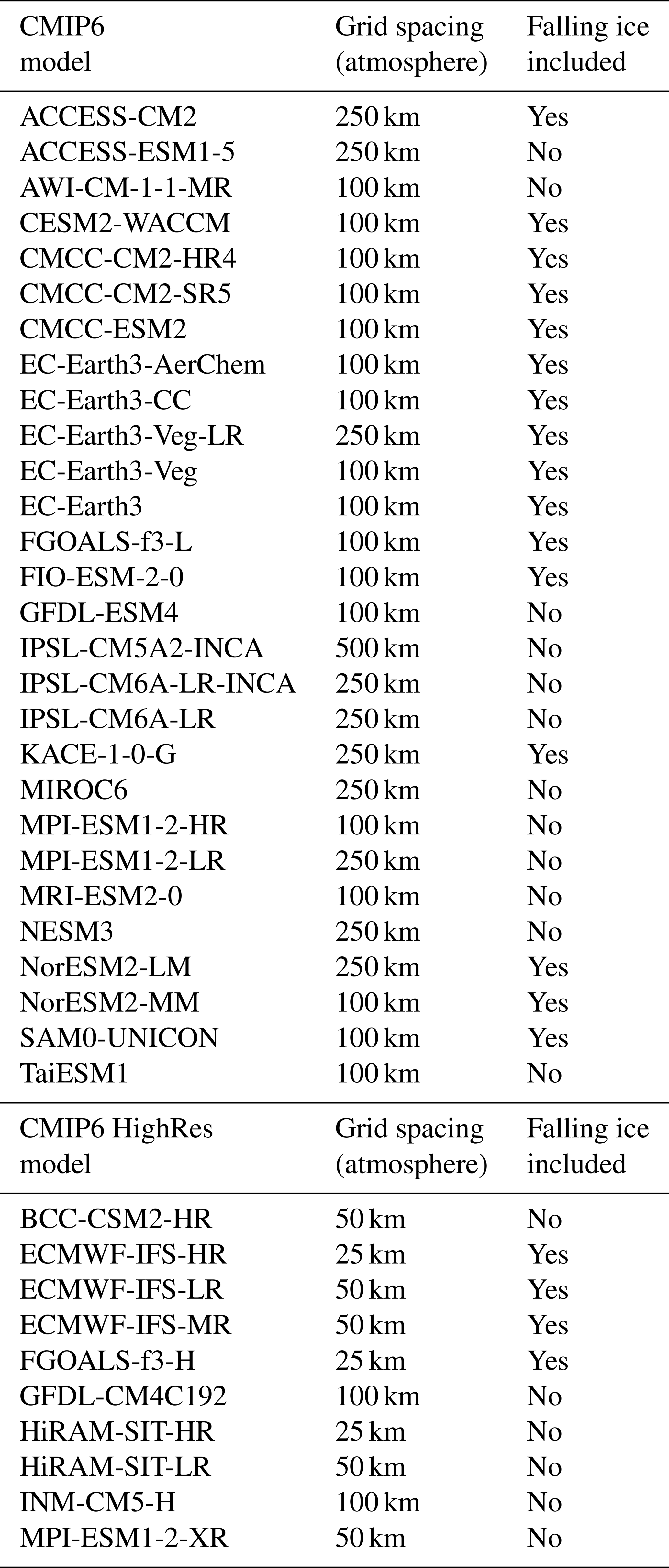
In this work, we use historical simulations from CMIP6 GCMs to assess their representation of atmospheric ice on global scales. The choice of the CMIP6 GCMs is based on data availability at the time of this study. 16 models are used, some of them with different model versions, resulting in 28 model outputs. Additionally, we complement the analysis with model output from the High Resolution Model Intercomparison Project (HighResMIP phase 1 or HighResMIP1) (Haarsma et al., 2016). That adds ten datasets to the analysis. The horizontal grid spacing of the simulations spans from 100–500 km for the atmospheric part of the CMIP6 GCMs and 25–100 km for the atmospheric part of the CMIP6 HighRes GCMs (see Table 1).

We use the variable clivi, defined as the atmosphere mass content of cloud ice, the so-called ice water path. In this study hereafter referred to as FWP. This variable includes precipitating frozen hydrometeors only when they affect the calculation of radiative transfer in the model, which is not the case for all models (Table 1).

Table 1 Model specifications of the CMIP6 historical and CMIP6 HighRes hist-1950 simulations used in the analysis: model name, horizontal resolution (approx. grid spacing at the equator) and whether the falling ice is considered in the radiative transfer and included in the FWP (“Falling ice included”). In all cases the configuration variant of the model is r1i1p1f1: realisation 1 (first ensemble member), initialisation method 1 (initial conditions of the piControl experiment), physics 1 (the standard physics setup of the model), forcing 1 (no additional forcing configuration).

2.3 Global storm-resolving models (GSRMs)

In recent years, with the growth of computational power, the possibility to simulate the atmosphere with a high resolution on global scales has become a reality (Stevens et al., 2019). These non-hydrostatic models typically utilize spatial grid spacings on the order of about 5 km and finer. This allows for the explicit simulation of the interaction between small, intermediate and large scales of motion, thereby avoiding the problems caused by the use of parametrizations (e.g., for deep convection) (Randall et al., 2003; Stevens and Bony, 2013; Stevens et al., 2019). The models with the capabilities to perform such simulations on global scales are known as GSRMs.

Table 2 Model specifications of the DYAMOND GSRMs simulations used in the analysis: model name, horizontal resolution (approx. grid spacing at the equator) and output frequency. Atmosphere models simulated atmosphere only, coupled models additionally simulated the ocean and land.

The Dynamics of the Atmosphere general circulation Modeled On Non-hydrostatic Domains (DYAMOND) intercomparison is the first intercomparison project of GSRMs. Since these models are able to simulate deep convection explicitly, they provide a more robust representation of the climate system and a more direct connection to high-resolution satellite retrievals (Stevens et al., 2019).

So far, two phases of DYAMOND have been carried out: (1st) DYAMOND Summer, and (2nd) DYAMOND Winter. In both of them, the GSRMs were run during 40 d periods: 1 August–10 September 2016 for the boreal summer, and 20 January–1 March 2020 for the boreal winter phase. The first ten days are considered spin-up time for the models and are excluded from our analysis. The models did run freely (no nudging towards re-analysis data was applied). Meteorological re-analysis provided by the European Centre for Medium Range Weather Forecasts (ECMWF) was used only to initialize the atmospheric state of the GSRMs. In this study, we use and compare the FWP from the models participating in the DYAMOND Winter phase. Since the GSRMs were freely run, they are not expected to reflect the real weather conditions during the simulated period. Therefore, in our study, the GSRMs outputs are analysed and compared with observations/retrievals from a statistical perspective.

Most DYAMOND models use one-moment microphysics schemes, which classify frozen water into cloud ice, graupel, and snow (Nugent et al., 2022). The data protocol of the DYAMOND intercomparison asked for including the vertical integral of cloud ice, snow and graupel. The models thus provide outputs of vertically integrated cloud ice (IWP), graupel (GWP), and snow (SWP) with output frequencies as can be seen in Table 2. To calculate the FWP we sum up the three vertically integrated hydrometeors mentioned before (IWP, GWP, SWP). That is, the DYAMOND dataset offers a first opportunity to compare the total amount atmospheric ice between different global models, a possibility used by e.g. Nugent et al. (2022); Ćorko et al. (2025). For the second (winter) phase of DYAMOND, 9 of 12 participating models met this suggestion. We chose the 9 DYAMOND models that provide all three parts of FWP (cloud ice, graupel, snow) for our study. In the case of IFS, graupel is not reported separately, but it is included in the snow category (SWP thus reflects both snow and graupel) (Peter Bechthold, ECMWF, personal communication, 2025).

3 Satellite retrievals

Frozen water path (FWP) from the 2C-ICE, DARDAR, AOP, and CCIC (CPCIR version) datasets (Sect. 2.1) are compared. These four products were selected because they all aim to retrieve the total ice hydrometeor mass, and their results should ideally agree perfectly. This is especially true for 2C-ICE, DARDAR and AOP, as they are all based on measurements by the CloudSat CPR radar, albeit the first two also incorporate the CALIOP lidar. The overall aim of the comparison is to establish the accuracy of global FWP datasets, to e.g. establish target ranges for the subsequent analysis of various atmospheric models.

The year 2015 was arbitrarily selected for the comparison. In Sect. 3.4 we argue that the derived differences are not critically dependent on the choice of year. During 2015, CloudSat measured only during the day part of its orbit and, as a consequence, all data in 2C-ICE, DARDAR and AOP are for a local solar time (LST) of about 13:30. CCIC data have been extracted along the CloudSat orbit by taking data within an interval of ±15 min around the same LST as CloudSat. Collocations were performed by performing a nearest neighbour interpolation of CCIC onto CloudSat geographical position, where the maximum distance of CCIC from CloudSat is 0.035° in latitude and longitude. Only data between 60° S and 60° N are considered, following the latitude coverage of the CCIC version used. To make the radar-based retrievals more comparable to the horizontal resolution of CCIC and the atmospheric models, the data from 2C-ICE, DARDAR, and AOP were averaged along track over about 6 km (four adjacent radar footprints) before the analysis. This averaging has no impact on regional and zonal means.

3.1 A sample scene

As an introduction to the satellite retrievals, Fig. 1 shows results for an individual scene. The first two panels show retrieved FWC from DARDAR and 2C-ICE to highlight some of their fundamental differences. AOP and CCIC also provide FWC, but are not shown since our focus is FWP.

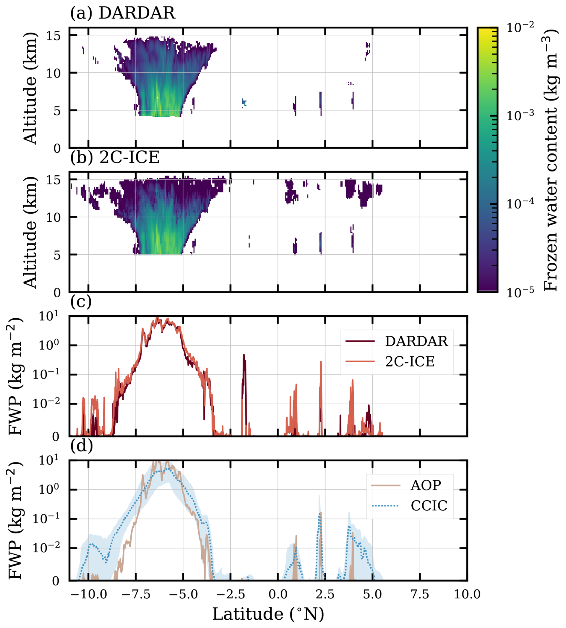
Figure 1 Example of collocated retrievals for a scene including deep convection (located between −7.5 and −5° N), observed on 28 August 2015. Panels (a) and (b) show the retrieved fields of frozen water content (FWC) for DARDAR and 2C-ICE, respectively. Panel (c) shows retrieved FWP from DARDAR and 2C-ICE, and panel (d) shows retrieved FWP from AOP nominal and CCIC. The shaded region in panel (d) represents the 90 % confidence interval for the retrieved CCIC FWP.

The FWCs from 2C-ICE and DARDAR agree broadly, but clear differences can be noticed. One example is the widespread thin clouds between 11 and 15 km found in 2C-ICE, but not in DARDAR. The FWP of these clouds reaches 10⁻² kg m⁻² (third panel). The radar-only AOP retrievals yield zero FWP for these clouds, indicating that the differences between DARDAR and 2C-ICE stem from how the lidar measurements are treated. Given the altitude, these clouds, if present, should consist solely of ice. CCIC appears to corroborate the presence of the thin clouds identified by 2C-ICE; however, it should be noted that CCIC is trained on 2C-ICE and may inherit its limitations.

DARDAR and 2C-ICE are more similar regarding the thin clouds found around 7 km. Still, here an opposing example can be noticed. Around −2° N DARDAR reports a FWP exceeding 0.1 kg m⁻², while 2C-ICE reports only an FWP of 10⁻² kg m⁻².

Further deviations are brought forward by the extensive convective system between −7.5 and −5° N. In particular, DARDAR reports non-zero FWC down to lower altitudes than 2C-ICE. In the case of DARDAR, all radar back-scattering measured at temperatures below 0 °C is assigned to ice hydrometeors, while for 2C-ICE this limit is set to −4 °C. On the other hand, the FWC of 2C-ICE tends to be higher in the mid-altitude region of the system, while DARDAR again is higher when reaching its upper parts. Integrated vertically, these differences largely cancel, and the FWPs of 2C-ICE and DARDAR end up being close. AOP gives matching values in the central section of the system but gives lower FWP in the anvil regions on both sides.

A general note on CCIC is its lower horizontal resolution, which explains the relatively smooth variation in FWP. The geostationary data used as input to CCIC have a resolution of about 5 km but, as these observations are highly indirect for determining FWPs, the retrievals incorporate spatial features in their estimation. Technically, this is achieved by making use of convolutions of the input image. As a result, the retrieval resolution deteriorates compared to that of the input data. For the thin clouds discussed above, CCIC tends to match the local peak values of 2C-ICE and thus overestimates the FWP averaged over each cloudy area. For the convective system, CCIC is on the low side compared to other datasets in the core region but gives higher FWPs, e.g., in the anvil around −7.5° N. As uncertainty estimates are not yet standard for machine learning products, one of CCIC's confidence intervals has been included. The test indicates that the quantile regression approach provides reliable values; the 90 % confidence interval largely brackets the DARDAR and 2C-ICE retrievals. The main exception is around −2° N, where 2C-ICE and DARDAR also disagree.

3.2 Collocation statistics

A more comprehensive view of the agreement between the collocated data is provided by Fig. 2. DARDAR is selected as the common reference for this comparison, but this shall not be taken as an indication that these retrievals are the most accurate. As data from 2015 are used, the results match daytime conditions only. More information can be obtained from lidar observations at night, when there is no interfering solar radiation.

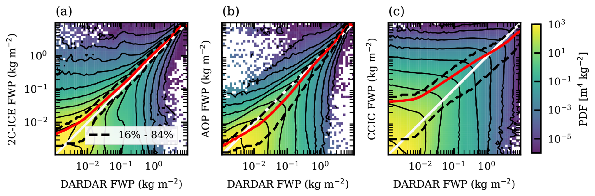
Figure 2 Joint probability distribution functions of collocated FWP retrievals. All panels show DARDAR FWP on the x-axis, with the y-axis showing 2C-ICE in panel (a), AOP nominal in panel (b), and CCIC in panel (c). The data are daytime-only collocations from 2015 between 60° S and 60° N. Black contour lines represent nine logarithmically spaced levels between 10⁻⁵ and 10³ m⁴ kg⁻². The red line represents the conditional mean. Black dashed lines represent the 16th and 84th quantile of the conditional distribution of the y-axis retrieval product FWP conditioned on DARDAR FWP.

Already Fig. 1 indicated that there are substantial differences between 2C-ICE and DARDAR, despite being based on the same input data. Figure 2a shows that the deviation at one location can exceed two orders of magnitude. However, such large deviations are rare, and 68 % of the retrievals are found along the 1:1 line between the two dashed lines. The distribution is somewhat shifted in the direction of higher 2C-ICE values, and the average of these retrievals is higher than that of DARDAR, as explored further below.

In Fig. 2b, it can be seen that there are fewer cases where AOP and DARDAR disagree by orders of magnitude. A contributing factor is that the nominal AOP retrievals apply the same temperature threshold for assigning radar back-scattering to liquid or ice particles as DARDAR (0 °C). For the uppermost range of FWPs, the highest densities and the conditional mean are found along the 1:1 line, and there is a symmetric pattern in general. For lower FWP (as reported by DARDAR), there is an asymmetry where higher densities and the conditional mean fall below the 1:1 line, indicating that AOP gives lower means than DARDAR in this range of FWP. This latter observation is partly explained by the fact that AOP does not consider any lidar data and thus misses the contribution from thinner clouds. However, there are situations where AOP is lower by 1 kg m⁻², and such large deviations show that other factors are also at play.

As expected, there is a high spread between CCIC and DARDAR on local scales (Fig. 2c). This can be attributed to the poorer horizontal resolution of CCIC. However, the CCIC retrievals are successful in the sense that the probability density exhibits a relatively symmetric pattern and that the full range of FWP values is found in CCIC. Except below $\mathrm{3}\times {\mathrm{10}}^{-\mathrm{3}}$ kg m⁻², the 1:1 line is inside the range spanned by the 16th and 84th percentiles. However, CCIC's deviations with respect to DARDAR are not fully symmetric, and the conditional mean lies above/below the 1:1 line below/above about 1 kg m⁻². The same pattern was found by Amell et al. (2024) when comparing to 2C-ICE, the reference dataset of CCIC.

3.3 FWP distributions

Moving to overall statistics, Fig. 3 shows the distribution of FWP inside each dataset. To aid comparison to earlier works, two versions are included. The data in Fig. 3a are normalised to be probability density functions (PDFs), p(FWP), i.e. their integrals are unity:

$$\begin{array}{}\text{(1)}& \underset{\mathrm{0}}{\overset{\mathrm{\infty }}{\int }}p\left(\mathrm{FWP}\right)d\mathrm{FWP}=\mathrm{1}.\end{array}$$

This type of distribution of FWPs has been reported by e.g. Wu et al. (2009), Eriksson et al. (2014), May et al. (2024). The PDFs in Fig. 3a vary over many orders of magnitude and steadily decrease with FWP. They have the same shape up to about 5 kg m⁻². Above this, the PDFs of 2C-ICE and AOP match well and are the highest, while the PDF of DARDAR drops off the quickest. CCIC is found in between.

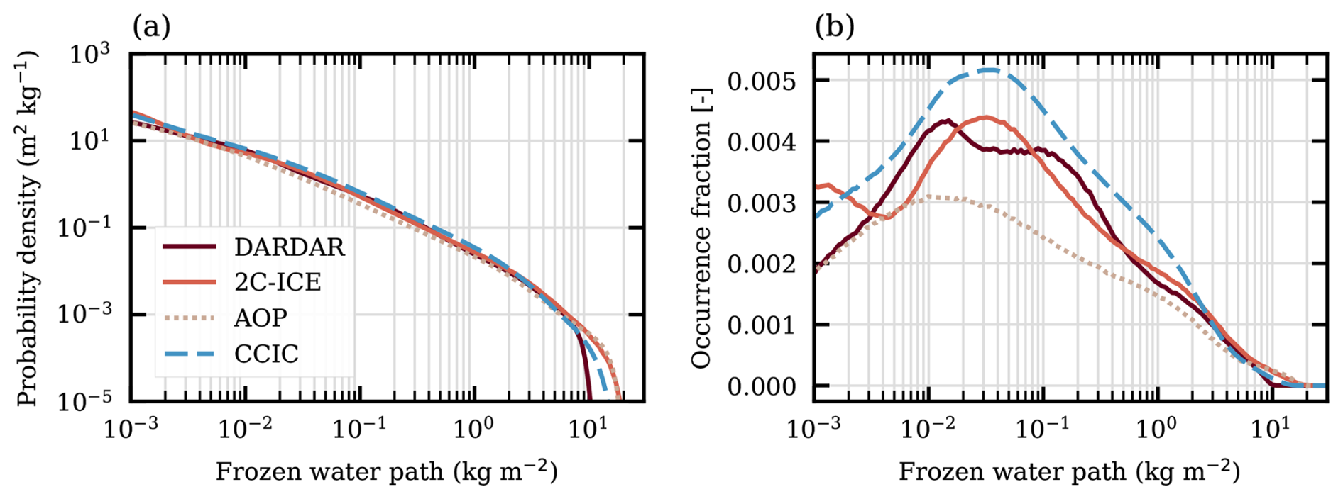
Figure 3 Distributions of retrieved FWP values from daytime observations during 2015 and for latitudes between ±60° N. The sampling of the CCIC dataset is centred around CloudSat LTAN with an interval of ±15 min. All cases (including FWP =0) are used in the normalisation. Panel (a) shows the overall probability distribution function. Panel (b) shows the logarithmically binned occurrence fractions (using 200 bins between 10⁻⁴ and 10² kg m⁻²).

In Fig. 3b, logarithmically binned occurrence fractions (log-OFs) are shown, o_i(FWP), i.e. their sums are unity:

$$\begin{array}{}\text{(2)}& \sum _{i=\mathrm{1}}^{n}o\left(\mathrm{FWP}\right)=\mathrm{1}.\end{array}$$

If the bins were equally sized (linearly), these distributions would have the same shape as the PDFs. FWP retrievals have been visualised as log-OFs by e.g. Hong et al. (2016), Sokol and Hartmann (2020), Atlas et al. (2024). When comparing the absolute values of both PDFs and log-OFs it must be considered if all FWP (as done here), or just cases above some threshold, are included. For log-OFs, the absolute values also depend on the selected bin sizes.

The log-OFs vary much less in magnitude. In fact, they are fairly constant between 10⁻³ and 1 kg m⁻², each varying by less than a factor of two. Compared to the PDFs, differences at lower FWPs stand out more clearly in the log-OFs. For FWP <5 kg m⁻², the largest discrepancy is found around 0.1 kg m⁻² where CCIC is about twice as high as AOP. On the other hand, the log-OFs of AOP and CCIC show consistency in both being smooth and unimodal, peaking between 0.01 and 0.04 kg m⁻². The peak values of the 2C-ICE and DARDAR log-OFs are generally found inside the same FWP range. However, these distributions are somewhat oscillating and a clear deviation between DARDAR and 2C-ICE occurs below $\mathrm{2}\times {\mathrm{10}}^{-\mathrm{3}}$ kg m⁻². The oscillations and the deviation at low FWP seen in Fig. 3b are also present when only considering retrievals from the tropical belt (Atlas et al., 2024).

The mean FWP can be derived from the PDF as

$$\begin{array}{}\text{(3)}& \stackrel{\mathrm{‾}}{\mathrm{FWP}}=\underset{\mathrm{0}}{\overset{\mathrm{\infty }}{\int }}p\left(\mathrm{FWP}\right)\mathrm{FWP}d\mathrm{FWP}.\end{array}$$

Thus, the product p(FWP) FWP shows how different FWP-ranges contribute to the mean FWP. It is interesting to note that log-OFs are directly proportional to this product, as the bin widths applied for the log-OFs are proportional to FWP. With this observation, we can deduce from Fig. 3b that FWP cases from below 10⁻³ kg m⁻² up to several kg m⁻² contribute significantly to the mean FWPs. That is, an observation system must cover about four orders of magnitude in FWP in order to provide a basis for correctly estimating global or local mean FWPs.

Table 3 Statistics of the satellite retrievals inside latitudes ±20° N (2015). AC is the anvil cirrus fraction (0.01 ≤ FWP < 1 kg m⁻²), CC is the convective core fraction (FWP ≥ 1 kg m⁻²), and the last column gives the 99.99th percentile in kg m⁻². Tropical convection has a considerable diurnal variation, in particular over land, and it is stressed that these fractions only are derived for the CloudSat passage time of 13:30 (LST). There are approximately 4.75 million samples per dataset, so about 475 samples exceed the 99.99th percentile.

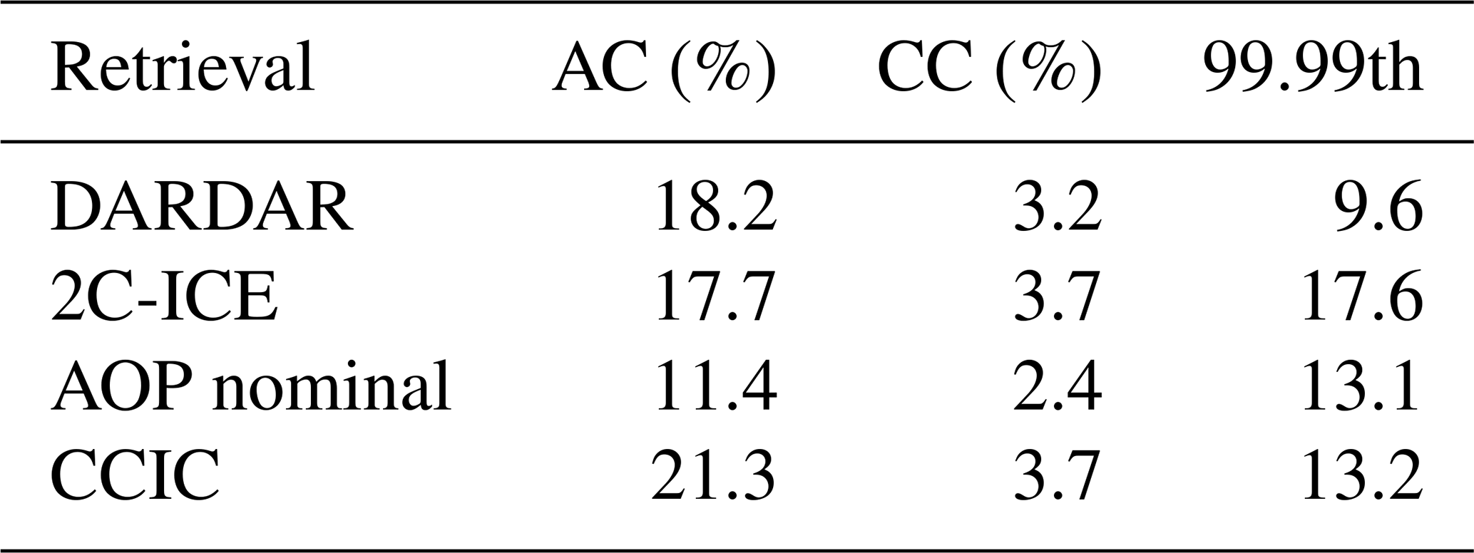
Sokol and Hartmann (2020) introduced a rough classification of tropical ice clouds: FWPs above 1 kg m⁻² are treated as convective cores (CC), FWPs below 10⁻² kg m⁻² are classified as thin cirrus, and intermediate values as anvil cirrus (AC). Table 3 reports AC and CC fractions according to this scheme, based on the satellite retrievals. 2C-ICE and DARDAR show the most consistent results, but the CC fraction of 2C-ICE is still 16 % higher than DARDAR (in relative terms). It is also noteworthy that the two datasets differ greatly for FWP above 10 kg m⁻², as indicated by their 99.99th percentile values. The deviations seen in Fig. 3a for high FWP are also valid for the tropical domain. An underestimation at high FWP is likely because, under such conditions, the radar pulse can be attenuated before reaching the bottom layers. The FWP that is still retrieved depends critically on how attenuation is estimated. For these situations, multiple scattering of the radar pulse is an additional consideration that is not yet covered (in contrast to the lidar side). A treatment of radar multiple scattering is part of at least one of the upcoming EarthCARE products (Mason et al., 2023).

Including lidar data, as done by DARDAR and 2C-ICE, helps detect thinner clouds, and the low anvil fraction of AOP can be understood as being radar-only. However, the information from the lidar should be of an indirect nature to constrain FWP >1 kg m⁻² and the low CC fraction of AOP can not directly be ruled out as being less trustworthy than the ones of 2C-ICE and DARDAR, increasing the possible span for the CC fraction downwards. CCIC has the highest fraction for both AC and CC. This can, at least in part, be attributed to the smearing effect discussed in conjunction with Fig. 1, and CCIC has likely a high bias in both CC and anvil “cloudiness”.

3.4 Mean values

The overall means of the datasets are found in Table 4. Since CCIC is trained on 2C-ICE, their mean FWPs are very close, around 0.14 kg m⁻². DARDAR and AOP also form a pair, with DARDAR achieving a mean FWP of 0.116 kg m⁻² and AOP achieving 0.115 kg m⁻². Both DARDAR and AOP apply a 0 °C liquid/ice threshold, but the close agreement between the two must still be considered unexpected since AOP applies a particle model that is entirely independent of the one used in DARDAR.

Table 4 Overall means of FWP between 60° S and 60° N (2015).

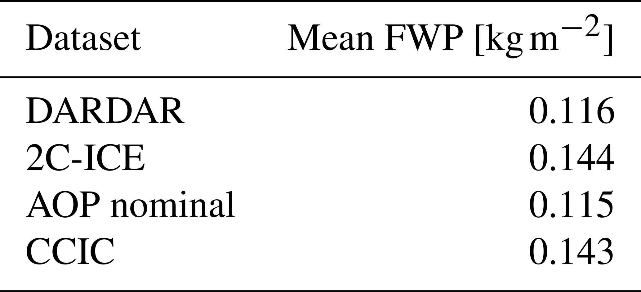
Figure 4 Zonal mean of FWP retrieved from daytime observations during 2015. The sampling of CCIC is centred around CloudSat LTAN with intervals of ±15 min.

DARDAR/2C-ICE is about 10 % below/above their combined mean. According to Fig. 6 of Pfreundschuh et al. (2025), the results on global mean FWP, including the difference between 2C-ICE and DARDAR, derived here for 2015, are representative of the complete CloudSat measurement period.

The zonal means found in Fig. 4 show that the agreement in mean FWP between 2C-ICE and CCIC, and between the DARDAR and AOP, is not limited to the overall mean. This pattern is also seen at each latitude range. For all latitudes, DARDAR, 2C-ICE and AOP are inside ±15 % of their combined mean (compared to ±10 % for the global mean). The same applies to regional means. Figure 7 of Pfreundschuh et al. (2025) shows that the spatial patterns of mean FWP from 2C-ICE, DARDAR and CCIC are very similar, and they only differ in the overall mean value. AOP also fits into this picture (not shown).

3.5 Sensitivity tests

The AOP framework is used here to test the sensitivity of overall means to several assumptions employed in the radar retrieval schemes. Performed tests and obtained changes in global mean FWP are reported in Table 5. For background information on AOP, see Sect. 2.1.2 and Appendix A.

Table 5 Change in overall mean FWP, ΔFWP, as a result of changes to the AOP retrieval scheme. The change in FWP is given as a percentage relative to the AOP nominal setup, i.e. the setup described in the first row of the table. The columns list in order: the particle habit applied, the particle size distribution (PSD) applied, if liquid water content (LWC) is considered in calculation of pulse attenuation, ice/liquid temperature limit (T), size of approximation for azimuthally random orientation (aARO) and the resulting ΔFWP. Remaining acronyms are described in the text.

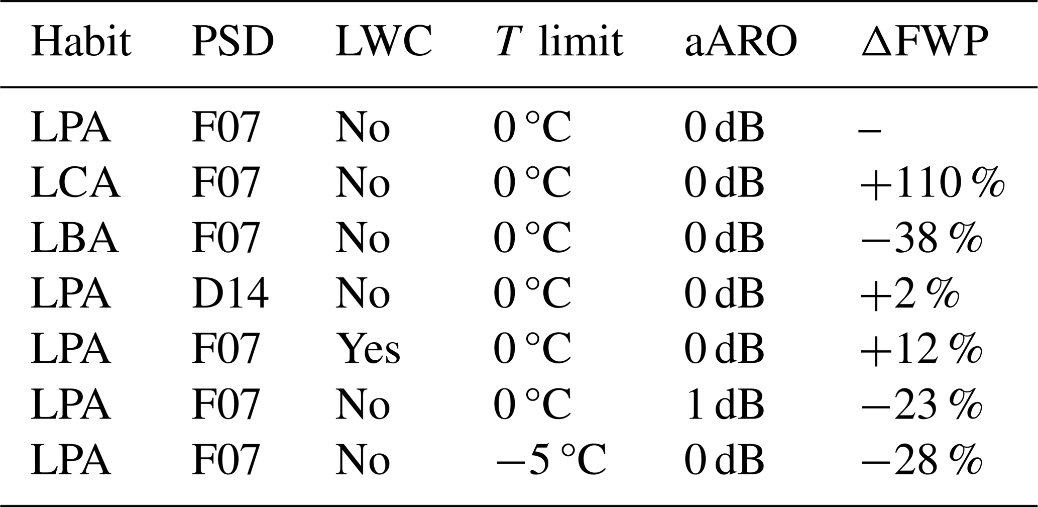
The first tests refer to changes in the particle model. Changing from the nominal large plate aggregate (LPA) to two other aggregate particle habits from Eriksson et al. (2018) affects the mean FWP drastically. The large column aggregate (LCA) gives less backscattering for a given particle mass. Reversely, a measured reflectivity then maps to a higher ice mass content and the global mean FWP more than doubles compared to when using LPA. Switching to the large block aggregate (LBA) has the opposite effect, as this habit constitutes a harder radar target, resulting in an FWP decrease of 38 %.

The second aspect of the particle models in AOP is the assumed PSD. Replacing Field et al. (F07, 2007) with Delanoë et al. (D14, 2014, used as in May et al., 2024) was found here to have a small effect, but this is not a general result since there could be a significant effect when used in conjunction with other habits. This is illustrated by Fig. 6 of Ekelund et al. (2020). This figure displays AOP retrievals for combinations of three PSDs and eight habits, serving as a complement to the results derived here.

In reality, both habit and PSD vary from position to position. However, satellite observations provide limited constraints on this variability, and the selection of particle model essentially boils down to finding the best average one. The nominal AOP particle model is primarily motivated by its use in RTTOV-SCATT to represent snow (Geer, 2021), making it widely used for assimilating passive observations at frequencies similar to those used by satellite-based cloud radars (94 GHz). The combination of F07 and LPA was singled out based on global observations, but the process assumed that the atmospheric data used (from ECMWF) had no biases, making the optimisation model specific. A similar study by Fox (2020), using another atmospheric model and restricted geographically, instead found F07 and LCA as the best particle model. The same combination was also found to be the best by Ekelund et al. (2020), based solely on satellite observations but limited to tropical conditions. The latter two studies found that LBA, in combination with F07, was a poorer option than the nominal particle model. For example, it deteriorates the agreement with the reflectivity-FWC relationship derived by Protat et al. (2016), compared to using LPA and LCA (Ekelund et al., 2020).

In summary, the question of a “one size fits all” ice particle model for the retrievals of concern remains an open question; however, the judgement is that the particle model selected for AOP (LPA) is more likely to yield a low bias than a high one.

Liquid cloud droplets are too small to cause significant reflectivity (for CloudSat CPR), but they still attenuate the radar pulse; however, this effect is neglected by DARDAR, 2C-ICE, and the nominal AOP setup. This results in a tendency towards under-estimation of ice mass. Including LWC from ERA5 (Hersbach et al., 2020) in the two-way attenuation of the radar pulse increases the overall mean with 12 %. The found value depends on how well ERA5 represents supercooled water, a quantity known to be poorly represented in atmospheric models (Komurcu et al., 2014; Korolev et al., 2017). There is also uncertainty in the microwave attenuation of supercooled water (Lonitz and Geer, 2019). The impact of neglecting LWC is the strongest at low latitudes.

All three retrievals involve non-spherical ice particles in their calculation of radar backscatter, but they all consider these to be totally randomly oriented (TRO). This is a simplification: ice hydrometeors tend to align their largest dimension horizontally (e.g. Hogan et al., 2002; Matrosov et al., 2005; Gong and Wu, 2017; Brath et al., 2020). Azimuthal random orientation (ARO) should still apply. By assuming TRO instead of ARO, the backscattering for a given ice mass is under-estimated, causing a high bias in the retrievals. Our test with AOP resulted in a 23 % decrease in FWP, assuming that particle orientation matches a change of 1 dBZ. Hogan et al. (2006) found that log ₁₀(FWC) is linearly proportional to 0.06 dBZ. This relationship gives a lower sensitivity, −15 % dB⁻¹. Marchand et al. (2013) found a median orientation effect of 2.4 dB, but this was based on data from a single measurement campaign.

As mentioned, cloud droplets do not generate a significant backscattering, but precipitation-sizes drops are still present at temperatures below 0 °C in updrafts. On the other hand, ice is found above 0 °C in falling melting particles. This raises a question of definition: shall ice in melting particles be included in FWP or not? Since including this ice fraction would further complicate the overall assessment, we set it aside for now. As for the particle model, the local variation can not be resolved, and the retrievals apply a global mean temperature threshold for delineating reflectivities generated between ice and (larger) liquid particles. The last test reported in Table 5 refers to changing the threshold temperature from 0 to −5 °C, a value that may be more realistic considering the discussion above and closer to the assumption in 2C-ICE (−4 °C). This change decreases FWP by 28 %.

Adding LWC increases FWP, but considering particle orientation and switching to a more realistic temperature threshold (ignoring melting ice) yields larger, opposing effects. Accordingly, the combined treatment of these three aspects in the nominal version of AOP likely results in a high bias. The bias is presumably significant.

3.6 Retrieval trueness

The DARDAR, 2C-ICE and CCIC retrievals come with case-specific errors that should be considered for single retrievals but cannot be easily mapped to averaged values. Assuming that averages are based on a large number of samples, the random component of local errors can basically be neglected. In this case, the retrieval trueness, i.e., the level of systematic errors, should be considered. Unfortunately, systematic retrieval errors are less well characterised than the random ones; it can be expected that provided retrieval errors do not include all systematic effects. In any case, no information is given on how local errors are partitioned between random and systematic sources.

In the lack of data to weight the different retrievals objectively, we argue for using the average of 2C-ICE and DARDAR as the best estimate of mean values, according to satellite retrievals. In the figures below, this centre level is determined by the mean for years 2007–2010, including both day and night retrievals. The mean is taken for the same part of the year as the data of concern. For example, the GSRM data in Sect. 5 cover only the month of February, and the satellite uncertainty range is correspondingly based on retrievals from February 2007 to 2010. The uncertainty around the centre level we estimate to be ±30 %. The reasoning for this choice is as follows.

Relative to their combined averaged values, the DARDAR and 2C-ICE means differ by about ±10 % (Sect. 3.4). It is likely overconfident to assume that these two retrievals bracket the true mean FWPs, given a high probability of additional biases.

For example, assuming that DARDAR has selected a close to optimal particle model, the last three rows of Table 5 still represent highly likely systematic errors. For example, the 0 °C threshold applied by DARDAR must be deemed to result in an overestimation of FWP. This is because liquid droplets large enough to cause radar backscattering exist at lower temperatures. The signs of the three effects are relatively certain, but their magnitudes are not. For the values applied in Sect. 3.5, these three error sources add up to −39 %. If this value is taken as a worst-case scenario and the estimate is halved, a 20 % overestimation in DARDAR remains possible. We also end up at around a 20 % overestimation if we assume that the two effects related to super-cooled liquid cancel each other perfectly, but consider the effect of particle orientation to be well captured by the test in Sect. 3.5 (giving −23 %).

The biases associated with the particle models can take either sign. The second row in Table 5 indicates that both DARDAR and 2C-ICE could be underestimating mean FWP by a factor of around 2. Considering that comparisons with airborne measurements show no strong biases (Deng et al., 2013; Heymsfield et al., 2017), and that the nominal AOP version is below 2C-ICE, we rule out such gross underestimations. Therefore, for simplicity, we assume a maximum systematic underestimation of 20 % in 2C-ICE due to a suboptimal particle model choice, resulting in a symmetric uncertainty range.

With a possible 20 % over-/underestimation by DARDAR/2C-ICE, we get a 30 % uncertainty with respect to the best estimate based on their combined mean (that is 10 % above/below the mean of DARDAR/2C-ICE). We cannot assign a likelihood to our uncertainty range; we just assume it to be on the conservative side. Accordingly, we expect that other datasets will fall within this uncertainty range in the comparisons below. For annual means between 60° S and 60° N, based on the results in Table 4, the target range is 0.091–0.169 kg m⁻² (0.130±0.039 kg m⁻²).

3.7 Emerging satellite retrievals

A second cloud radar has now been launched: The Cloud Profiling Radar (CPR) onboard EarthCARE (Wehr et al., 2023). EarthCARE's CPR is a 94 GHz single-frequency radar, like CloudSat's CPR, and retrievals remain highly sensitive to the assumed particle model. However, there are several improvements. This new radar has a higher sensitivity, extending the retrieval coverage to lower FWPs, and it has the capability to measure vertical velocities, providing additional input for retrieval schemes with respect to e.g. a riming factor (Mason et al., 2023). At the time of writing, none of the EarthCARE products have reached a stable version and are not considered.

CCIC demonstrates that machine learning unlocks new possibilities, and we anticipate seeing improved FWP estimates based on existing passive measurements. A product similar to CCIC, but with limited spatial coverage, is presented by Jeggle et al. (2025). Continuous production using an updated version of the SPARE-ICE (Synergistic Passive Atmospheric Retrieval Experiment-ICE) algorithm (Holl et al., 2014) has just started. SPARE-ICE is a dataset of FWP retrievals derived exclusively from passive microwave and infrared observations using the Microwave Humidity Sounder (MHS) and the Advanced Very High Resolution Radiometer (AVHRR) on board NOAA-18, NOAA-19 and the MetOp satellites. The retrievals are performed using machine learning, with the model trained on 2C-ICE data collocated with MHS and AVHRR observations from NOAA-18.

Passive retrievals will also benefit from data in a new wavelength (λ) region – the sub-millimetre. The Ice Cloud Imager (ICI) is an upcoming mission in this direction, dedicated to measuring ice hydrometeor properties (Eriksson et al., 2020). This sensor, scheduled for launch in 2026, will conduct observations at higher microwave frequencies than those currently used, thereby enhancing sensitivity to ice cloud mass (Evans and Stephens, 1995; Jimenez et al., 2007). ICI will have channels up to 664 GHz (λ=0.45 mm), but the Arctic Weather Satellite (AWS, Eriksson et al. (2025)), launched in 2024, already provides a first glimpse of ice clouds at the lower end of the sub-millimetre range with four channels around 325 GHz (λ=0.9 mm).

These later emerging retrievals, based on passive data, are exemplified in Fig. 5. CCIC is included and serves as a reference to the results found above. The AWS retrievals are made following May et al. (2024). It is noteworthy that the AWS algorithm does not involve any other retrievals (in contrast to CCIC); instead, the machine learning is based on physical simulations. As both CCIC and SPARE-ICE are trained on 2C-ICE data, it is not surprising that their zonal means align closely south of 15° N. However, there is a clear disagreement in the remaining part of the northern hemisphere, indicating that machine learning based on collocations has specific issues to consider. For this northern range, there is strong agreement between SPARE-ICE and AWS. The latter two retrievals are for these latitudes at the lower end of the expected range, but CCIC is also relatively low compared to the historical data, indicating that the mean FWP was low during the two months considered. Some annual variations are to be expected for means over relatively short time periods. In summary, the AWS and SPARE-ICE data show acceptable agreement with the reference, despite being emerging datasets.

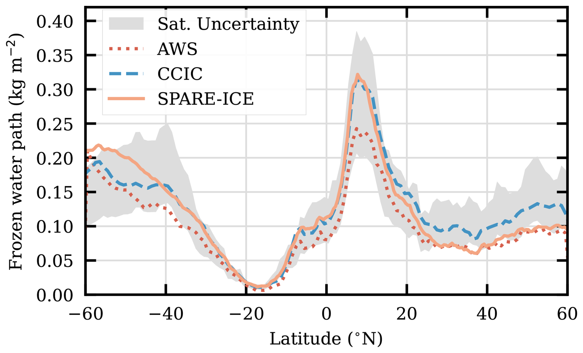
Figure 5 Zonal mean, for July and August 2025, of three retrievals based on passive observations. The CCIC data have been sub-sampled to the local solar times observed by AWS (approx. 10:30 and 22:30). The grey area represents the expected range according to CloudSat-based estimates covering 2007–2010 (see Sect. 3.6 for details).

4 General circulation models

In the following, we compare the FWP for a selection of CMIP6 and CMIP6-HighRes models (historical simulations). The variable used for the analysis (clivi) refers to the atmosphere mass content of cloud ice and does not always include precipitating frozen hydrometeors (Sect. 2.2), i.e., snow and graupel. In other words, not all ice is represented in the FWP for all models, and we can expect lower values from the CMIP6 analysis compared to satellite retrievals. However, we still compare these models with observations following Waliser et al. (2009), Jiang et al. (2012), Li et al. (2012, 2020), and others. More details on the specific models and the inclusion of precipitating hydrometeors can be found in Table 1. Note that in the following, the overall assessment is based on means within the 60° S–60° N latitude range to enable a proper comparison with the satellite retrievals.

4.1 Mean values

We first explore quasi-global mean values within the 60° S–60° N latitude range. Figure 6 shows that, in both groups of models, the mean FWP is within similar ranges: from 0.011 to 0.088 kg m⁻² in the CMIP6 historical simulations, and from 0.011 to 0.090 kg m⁻² in the CMIP6-HighRes simulations. This means that the models with the largest FWPs have values around 6 to 8 times higher than those with the smallest FWPs. This overall behaviour remains largely unchanged when all latitudes are included (not shown). Waliser et al. (2009), in a similar comparison using CMIP3 models, found differences of up to a factor of 20 between the models with the highest and lowest FWP values (Fig. 1d in Waliser et al., 2009). However, this large spread was primarily due to two models with markedly high FWPs. When those outliers were excluded, the remaining models showed differences of about a factor of 6 – comparable to our findings. Moreover, although not explicitly quantified in Waliser et al. (2009), the global mean FWPs of these models appear to fall within a similar range to those we found in our study. It is noteworthy that there is no clear separation between models that just include cloud ice in the reported FWP and those that also add falling ice. For example, the two model categories are represented at both ends of the FWP range (Fig. 6).

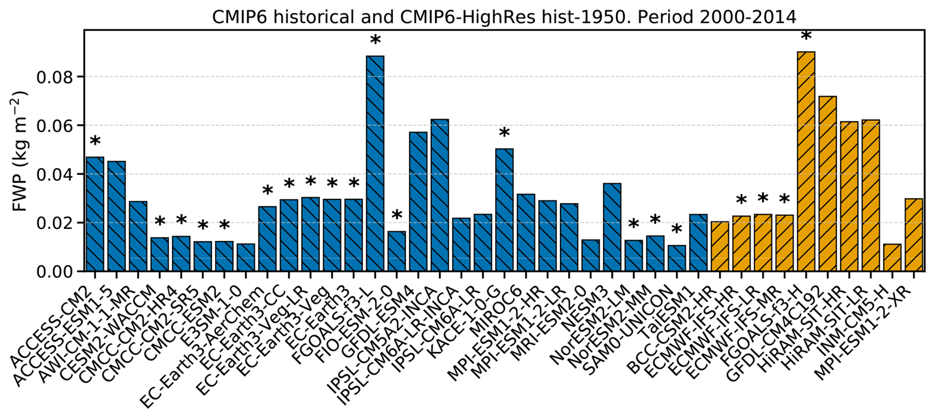
Figure 6 Average of monthly FWP means, between latitudes 60° S and 60° N, during the period 2000–2014 for the CMIP6 historical simulations (bars in blue with stripes descending), and CMIP6 HighRes hist-1950 simulations (bars in orange with stripes ascending). Models including falling ice in their FWP are marked with an asterisk (*).

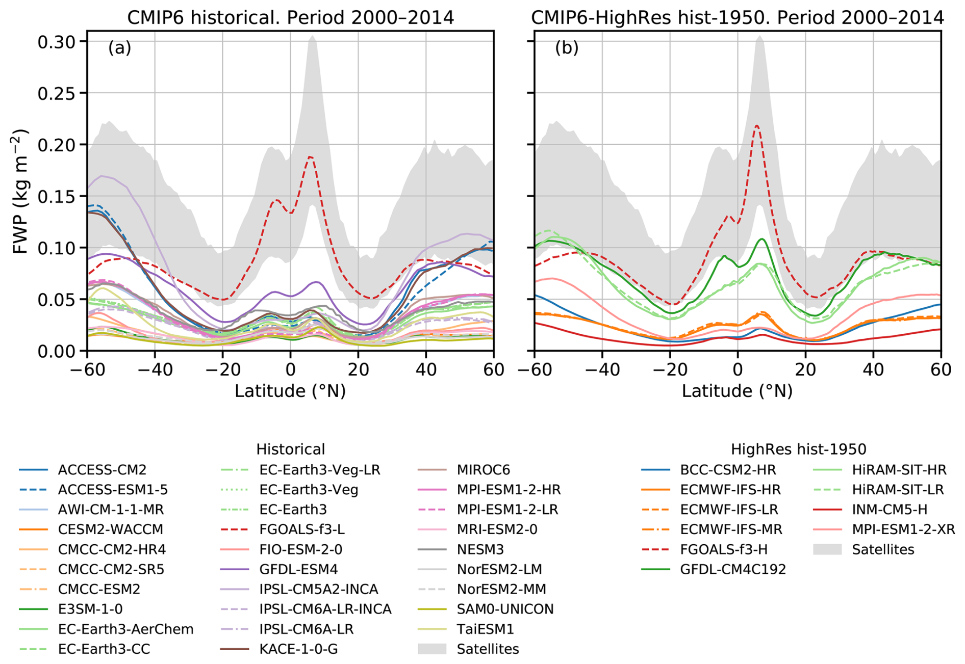
Figure 7 Zonal means of monthly FWP means during the period 2000-2014 for (a) CMIP6 historical simulations, and (b) CMIP6 HighRes hist-1950 simulations. The grey area represents the expected range according to CloudSat-based estimates covering 2007–2010 (Sect. 3.6).

To further explore the differences, we calculate the FWP zonal means and compare these with satellite retrievals (Fig. 7). Nearly all models participating in the CMIP6 and CMIP6-HighRes underestimate the FWP when compared to satellite retrievals. In the historical simulations (Fig. 7a), there is a large spread in FWP values across the mid and high latitudes, with some of the models approaching or falling within the satellite retrieval range (e.g. IPSL-CM5A2-INCA, ACCESS-ESM1-5, ACCESS-CM2 and KACE-1-0-G). On the other hand, the values are clustered below 0.05 kg m⁻² in the tropics, and are substantially smaller than the satellite retrieval. The only exception is the FGOALS-f3-L model, whose values in the tropics and subtropics fall within the satellite range. In the CMIP6-HighRes simulations (Fig. 7b), the high-resolution version of the model FGOAL (FGOALS-f3-H) also produces FWPs values in the tropics and subtropics that fall within the satellite range. Both FGOALS simulations (for CMIP6 and CMIP6-HighRes) produce very similar FWPs. The remaining models appear to be divided into two distinct groups, with one group – HiRAM-SIT-HR, HiRAM-SIT-LR, and GFDL-CM4C192 – exhibiting higher mean FWPs across all latitudes and aligning more closely with satellite retrievals than the other models.

As for the quasi-global means, no systematic difference between the models including falling ice or not is found and for most models a small relative latitudinal difference in low/high FWP values can be seen, i.e. a model with low quasi-global FWP means shows low zonal mean FWP values over the whole latitude range. Another interesting feature is that the FWPs of the simulations performed with the same model but at different resolutions (e.g., ECMWF and HiRAM) do not differ substantially. Furthermore, the combined information from Table 1 and Fig. 7b does not suggest an improvement in the simulated FWPs when the grid spacing decreases from 100 to 25 km. This is not particularly surprising since at those resolutions many processes in these models (e.g., deep convection and ice-phase processes) still need to be parametrized and the model physics is the same for the models participating in both, CMIP6 and CMIP6-HighRes.

Previous research comparing GCMs with observations has identified several of the features we highlight above. For instance, Komurcu et al. (2014) also reported an underestimation of FWP in GCMs (from the IPCC (Intergovernmental Panel on Climate Change), AR5) compared to observations, which is consistent with the FWP range they obtained (as described above). Moreover, Eliasson et al. (2011) found that, over the tropical oceans, the FWP in half of the six GCMs from the IPCC AR4 they evaluated fell below or well below the uncertainty range of satellite retrievals. In our case, this underestimation applies to most models across the entire tropical region, including both land and ocean areas.

4.2 Trends

Time series of monthly quasi-global mean FWP covering 35 years are found in Fig. B1. Linear fits of these time series give trends between −1.0 and +0.5 % per decade. This lack of clear trends is consistent with the CCIC data record, which also indicates a basically constant global mean FWP since 1983 (Pfreundschuh et al., 2025). On the other hand, CCIC and other datasets show that there have been clear regional trends in mean FWP. Here, we disregard the exact values of regional trends and instead investigate the agreement among GCMs regarding these trends. To minimise the impact of differences in global mean FWP, trends are reported relative to local means. This approach was adopted by Pfreundschuh et al. (2025), and a high level of agreement was obtained for trends between CCIC and ERA5, even though the latter dataset does not report all ice mass.

Regional FWP trends for all models are found in Figs. B2 and B3. There is a clear spread in the trends between the models. One feature worth highlighting is the trend in the eastern Pacific ITCZ. In this region, some models predict a negative tendency, which is in line with the 40-year trends of CCIC and PATMOS-x in Pfreundschuh et al. (2025) (their Fig. 11), but in disagreement with the corresponding trends for ISCCP and with the 20-year trends for all datasets in Pfreundschuh et al. (2025) (their Fig. 10). However, other models, like the FGOALS-f3-L, exhibit a positive trend in this region. Overall, no clear relationship emerges between the features observed in the trends and the model characteristics investigated (i.e. the spatial resolution or inclusion of falling ice).

4.3 Annual cycles

Variations of global mean FWP with a period of one year can be discerned in Fig. B1. To investigate this further, long-term mean annual cycles were derived and are displayed in Fig. 8. CCIC indicates a semi-annual variation with maxima and minima at about 2 % above and below the annual average. The maxima occur about one month before the summer/winter solstices. The annual cycles of the GCMs vary. Compared to CCIC, the amplitude of the models' cycles is, in general, higher, with peak-to-peak amplitudes of up to about 15 %, but there are also some models with weaker cycles. Most models exhibit a semi-annual pattern similar to CCIC, but there are also models where the peak during boreal spring dominates. For the boreal spring, there is also a tendency for the models to peak about one month earlier (April–May) than CCIC (May–June). In summary, most models provide a fair representation of the annual cycle in global mean FWP, but some notable deviations are evident.

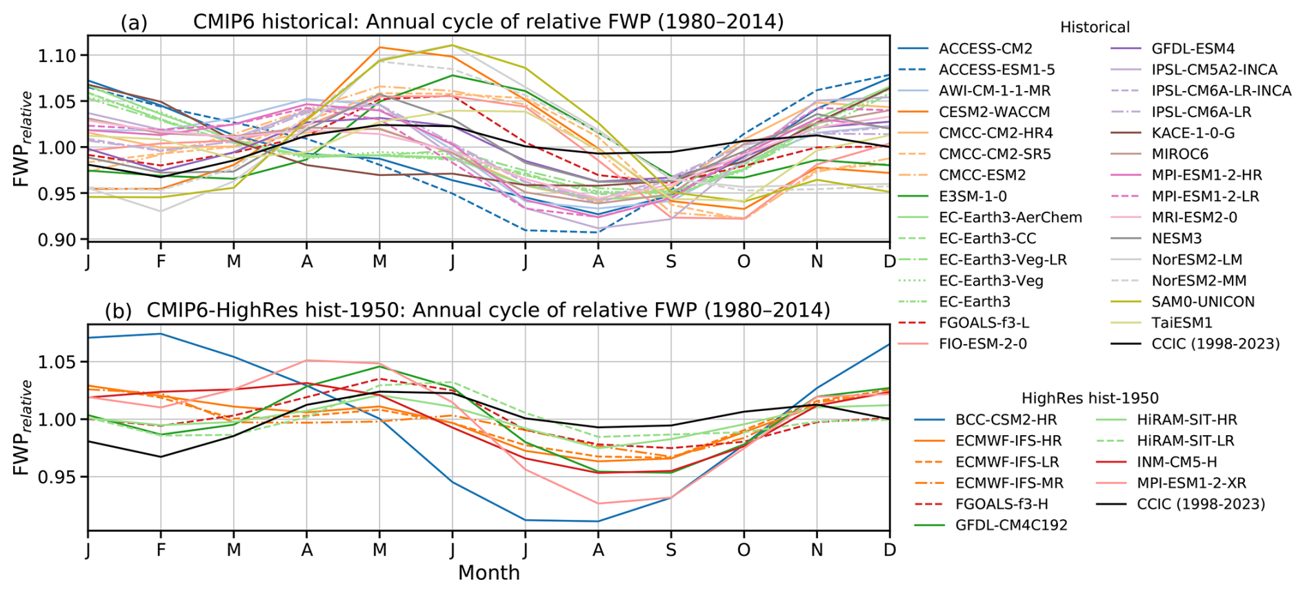
Figure 8 Annual cycles of relative FWPs (FWP_relative) between 60° S and 60° N, calculated for each model as the ratio of monthly mean FWP to the mean FWP over 1980–2014. Results are shown for (a) CMIP6 historical simulations and (b) CMIP6 HighRes hist-1950 simulations. The annual cycle of FWP_relative for CCIC over 1998–2023 is also shown in both panels for comparison.

5 Global storm-resolving models

In this section, FWP in global storm-resolving models (GSRMs) is assessed. The aim is to explore the general capabilities of this new type of models. Details of individual models are brought forward to indicate issues to be resolved, not to rank the models in any manner. The GSRM data is taken from the DYAMOND model intercomparison project and covers February 2020 (i.e. the spin-up period is not included, Sect. 4). Following the satellite section, we limit the overall assessment to 60° S–60° N. This is complemented with a dedicated section on the Tropics (20° S–20° N).

5.1 Overall statistics

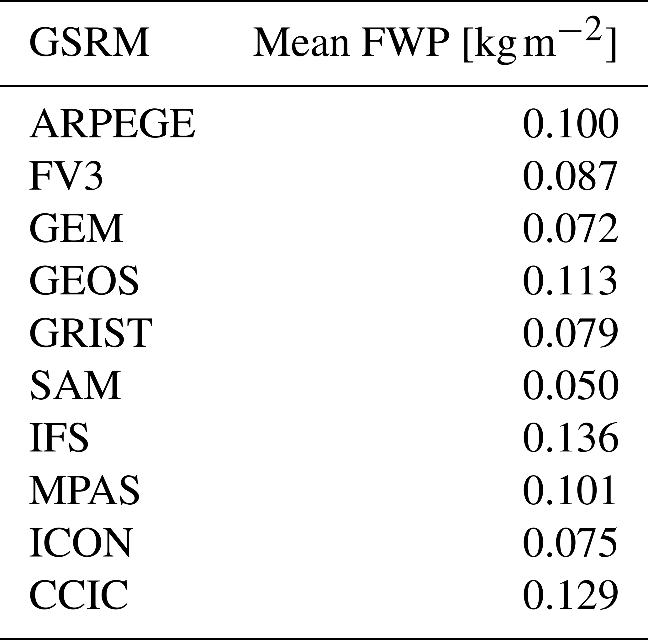
The (quasi-global) mean FWPs of the GSRM models are shown in Table 6. Given that these models incorporate advanced features intended to improve the representation of the climate system compared to the GCMs (see Sect. 2.3), we expect their FWPs to show better agreement with observations. This is the case. The target range for these means derived in Sect. 3.6 is 0.091–0.169 kg m⁻². ARPEGE, GEOS, IFS and MPAS are inside this range. The corresponding CCIC value is included in Table 6. CCIC is here about 10 % lower than in Table 4, indicating a lower global mean for this month than the full annual mean used as a reference. If decreasing the target range by 10 %, which sets a lower limit of approximately 0.082 kg m⁻², also FV3 ends up inside the range. Among the remaining models, GEM, GRIST and ICON lie relatively close to this lower bound, while SAM reports the lowest value at 0.050 kg m⁻².

Table 6 Means FWP between 60° S and 60° N of considered GSRM model runs (covering February 2020). The mean of CCIC for the same area and time period is included, as a reference.

For a comprehensive view of the spatial distribution, Fig. 9 compares the model ensemble mean FWPs with corresponding CCIC satellite retrievals. Global distributions for the DYAMOND summer phase (winter phase used in this work) are found in Fig. 1 of Ćorko et al. (2025).

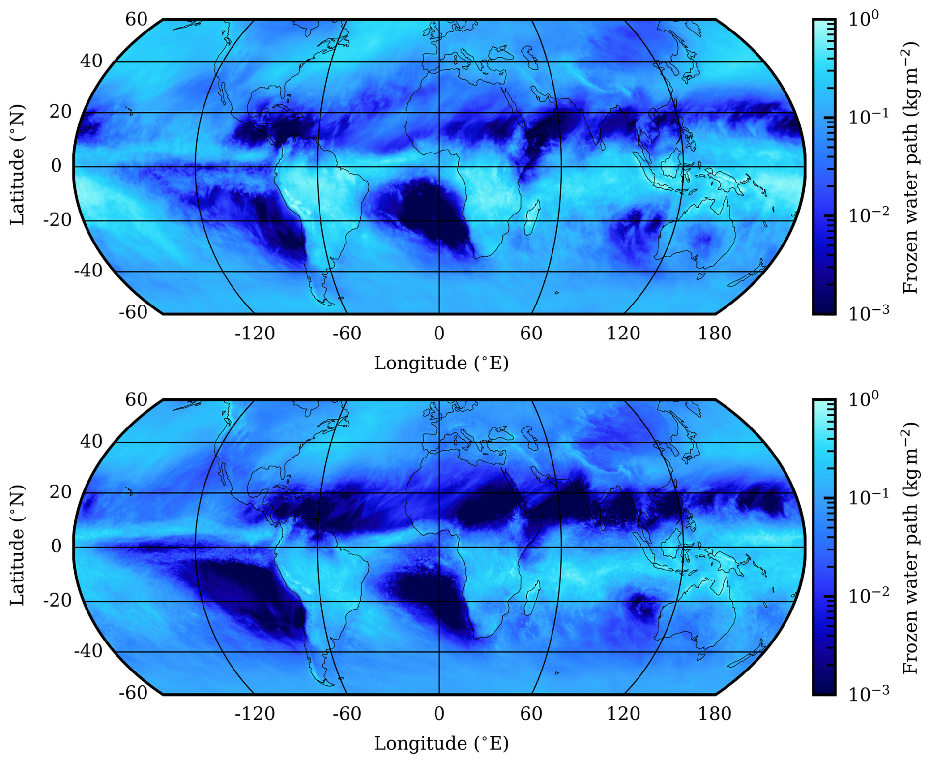
Figure 9 Gridded (1° resolution) mean FWP for February 2020, for CCIC (top panel) and averaged over the nine considered GSRMs (lower panel).

As discussed above, the model ensemble exhibits a lower global mean FWP compared to CCIC. Nevertheless, disregarding this offset in the mean, the agreement shown in Fig. 9 can be considered strong. The spatial patterns of mean FWP in the models generally align well with those derived from observations, despite the fact that the GSRMs were not nudged to reproduce the actual weather during the analysed period. For instance, the signatures of the Intertropical Convergence Zone (ITCZ), as well as the Andean, Zagros, and Himalayan mountain ranges, are strikingly similar in both panels. On the other hand, the model ensemble shows more extensive regions of very low mean FWP across the tropics and subtropics.

Zonal means from the GSRMs are shown in Fig. 10. The majority of models produce values within the satellite-derived range or are around its lower bound. The SAM model consistently exhibits the lowest mean FWP across most of the latitudes. Interestingly, Atlas et al. (2024) found that, in SAM, the SAM1MOM microphysics scheme – also used in the DYAMOND simulations – produced the lowest FWP among several available microphysics schemes. This suggests that the selection of this microphysics scheme is likely the primary factor contributing to the relatively low FWP values in SAM's DYAMOND simulations. In the tropics, IFS stands out by having a mean FWP about double as high as any other model around 10° S. IFS shows a similar behaviour in the DYAMOND summer phase (Ćorko et al., 2025, Fig. 2).

In summary, compared to the GCMs, the spread among the GSRMs is relatively small. This is partly due to the consistent definition of FWP applied across all models, but it also represents a positive indication of their ability to bracket the mean FWP of Earth's atmosphere.

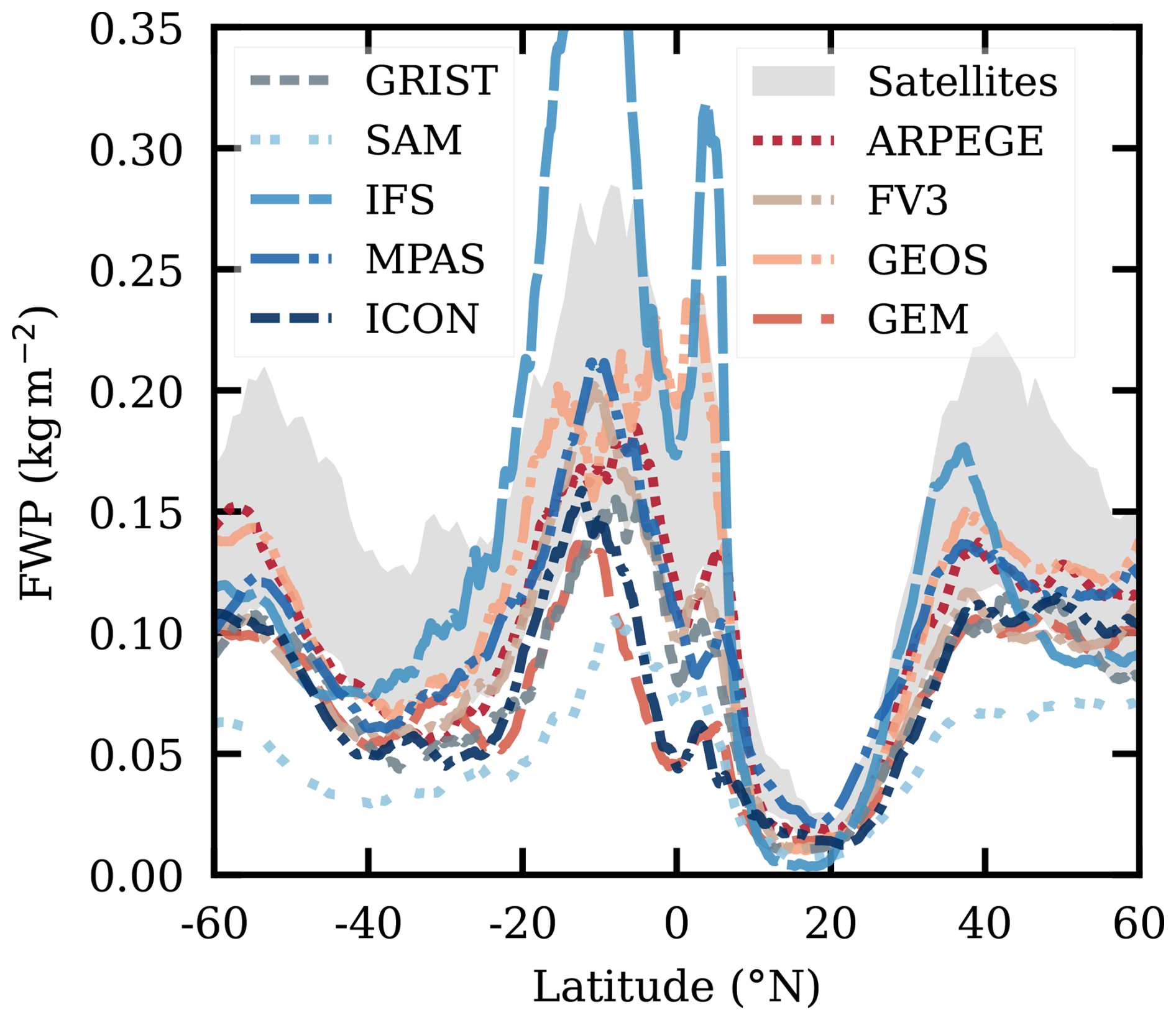
Figure 10 Zonal mean FWP of the GSRM models (February 2020). The grey area represents the expected range according to CloudSat-based estimates covering 2007–2010 (Sect. 3.6). The primary peak of the IFS-model is cut off in an attempt to improve visual clarity for all other models. It has a maximum FWP value of 0.46 kg m⁻² at 9.5° S.

Figure 11 provides an overview of individual FWP values. Aside from discretization artefacts, the models exhibit similar distributions, generally peaking around 0.02 kg m⁻². The main exception is FV3, that peaks around $\mathrm{3}\times {\mathrm{10}}^{-\mathrm{3}}$ kg m⁻². The same bin size has been applied in Figs. 11 and 3b and the results are comparable. Model and observational distributions agree well, most closely at high occurrence fractions where they exhibit similar peak values. The models tend to be on the high/lower side at the lower/higher FWPs.

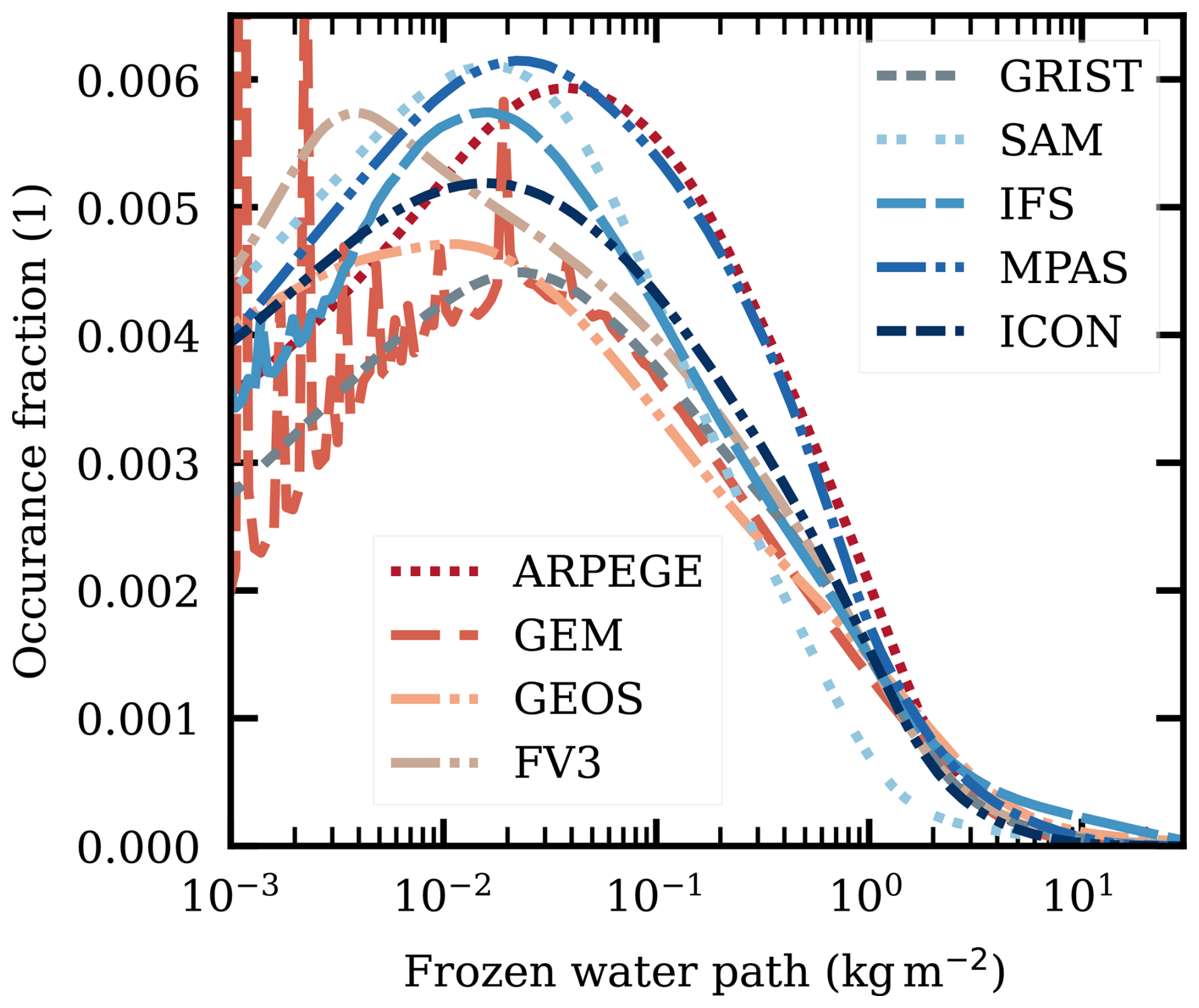
Figure 11 Logarithmically binned occurrence fractions (log-OF) of each model's FWP between 60° S and 60° N (February 2020). The spikes for some models are caused by discretization of the output.

As explained in Sect. 2.3, the output of the GSRMs distinguishes between ice water path (IWP), snow water path (SWP) and graupel water path (GWP), with the FWP defined as the sum of these three components. This detailed output allows to compare the partitioning among ice-phase hydrometeors in the GSRMs, an analysis that is not possible with the GCMs due to the absence of these specific output variables. The IWP, SWP and GWP fractions for quasi-global data are visualised in Fig. 12. These fractions were also calculated over other latitude ranges, but since only small variations were found these results are not presented. The most clear difference in fractions between the extra-tropics and the tropics, is a somewhat higher graupel fraction in the latter case, at the expense of cloud ice. An exception is the SAM model, that exhibited the opposite behaviour. The snow fractions stayed unaffected by the latitude limits applied (with the exception of IFS that does not distinguish between snow and graupel).

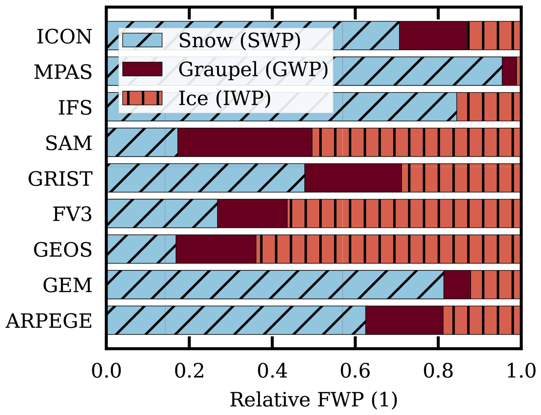
Figure 12 Relative fraction of ice, snow and graupel to the total frozen water, for each GSRM model. Compiled using all data between 60° S and 60° N (February 2020). For IFS, snow incorporates the graupel category.

Although the fractions of FWP experience only minor variations across latitude changes within each model, there is a clear lack of agreement between the models. The fractions vary as follows: snow 17 %–95 %, graupel 3 %–32 %, and ice 1 %–64 %. There is no obvious relationship between the category fractions and mean FWP. For example, SAM and GEOS have similar fractions, but SAM is the model with lowest FWP and GEOS is around or above average in zonal mean values.

In summary, Fig. 12 illustrates that there is no common view among the GSRMs on the fractioning between cloud ice, snow and graupel. It is outside the scope of this work to explore this further. However, presumably, both basic definitions of the meaning of these ice categories and direct model shortcomings contribute to this poor agreement.

5.2 The tropical region

The higher horizontal resolution of GSRMs, in comparison to GCMs, is expected to be especially beneficial for the representation of tropical deep convection, and, accordingly, many studies making use of the DYAMOND database are focused on the tropical region (e.g. Christensen and Driver, 2021; Su et al., 2022; Nugent et al., 2022; Turbeville et al., 2022). In this section, we follow the same line and present statistics on the impact of deep convection.

The high end of the distribution of tropical FWP (all-day, February 2020) of each model is summarised Table 7. For the same analysis of the satellite retrievals in Sect. 3.3, the data were taken from 2015 and only cover local solar times around 01:30. The results for CCIC in Tables 3 and 7 for three statistical measures are fairly similar ($\mathrm{21.3}/\mathrm{24.9}$, $\mathrm{3.7}/\mathrm{4.0}$, and $\mathrm{13.2}/\mathrm{12.9}$). Nevertheless, the different time coverages should be kept in mind in the following discussion around Table 7.

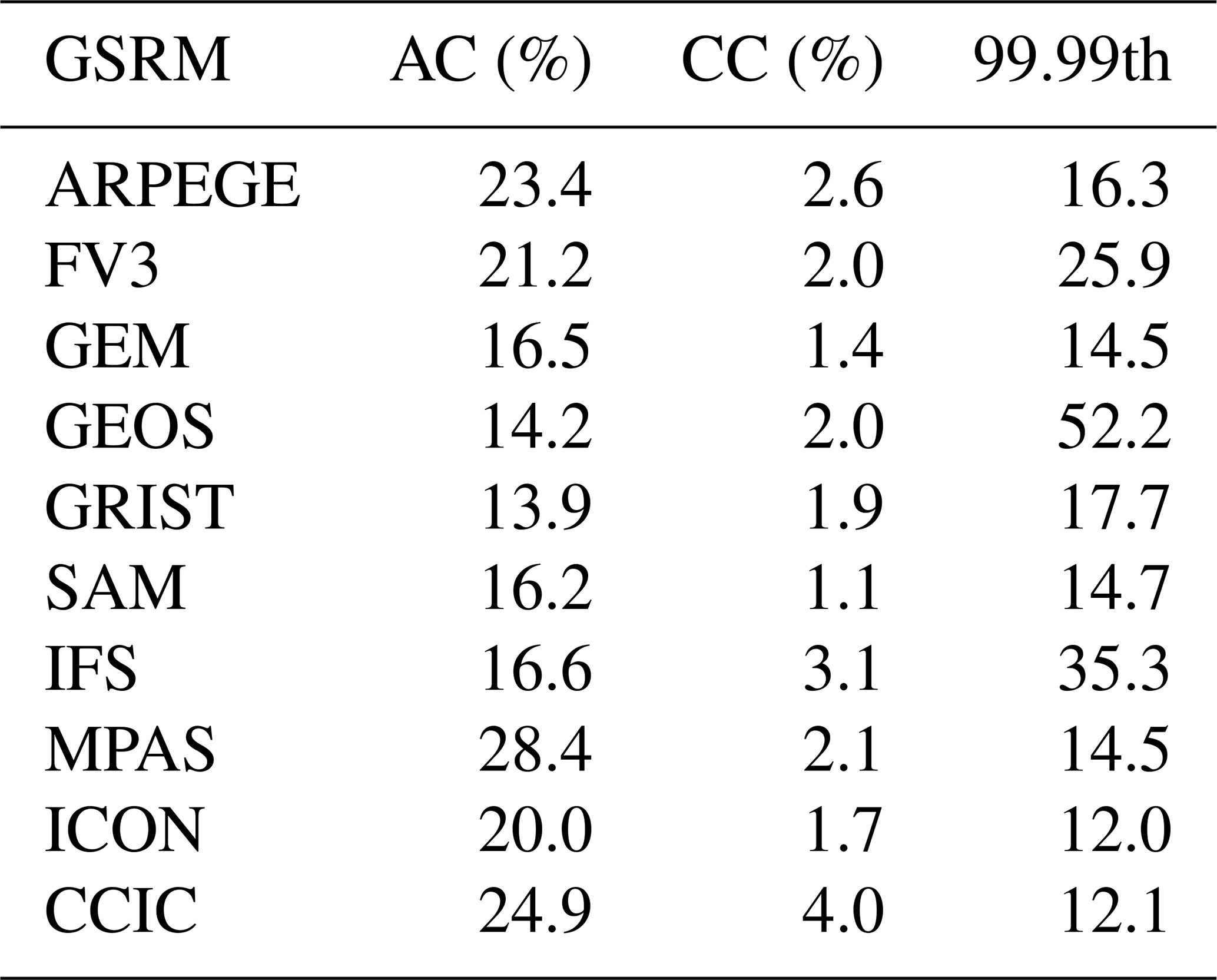
There is a considerable spread among the models in their 99.99th percentile, with values from 12.0 kg m⁻² (ICON) to 52.2 kg m⁻² (GEOS). The corresponding range for the satellite retrievals is 9.6–17.6 kg m⁻², but a low bias in these values is likely due to the high attenuation of the radar signal at very high FWPs (Sect. 3.3). Accordingly, all the models' 99.99th percentiles can be considered as reasonable. In any case, none of the models exhibits an apparent deficiency in simulating very high FWP values.

Despite reaching FWP values exceeding 10 kg m⁻², the models tend to have low CC fractions. None surpasses the CC fraction derived from DARDAR of 3.2 %, and they fall even further below the 3.7 % reported by both 2C-ICE and CCIC (Table 3). The closest is IFS at 3.1 %. The CC fraction of AOP is considerably lower (2.4 %), but, aside from IFS, only ARPEGE exceeds this value. The CC fractions correlate to some extent with the models' overall mean FWP. The models' AC fractions vary with a factor of 2, between 14 % and 28 %, but they are fairly well centred around the observations.

Table 7 Statistics of GSRM FWP inside latitudes ±20° N (Feb 2020). AC is the anvil cirrus fraction (0.01 ≤ FWP < 1 kg m⁻²), CC is the convective core fraction (FWP ≥ 1 kg m⁻²), and the last column gives the 99.99th percentile in kg m⁻². The CCIC-based statistics for the same area and time period is included, for reference.

The remainder of this sub-section is focused on the organization of convection. The primary manner to track tropical mesoscale convective systems by satellite data is through measured infrared radiances (Feng et al., 2025), but it has been shown that FWP from CCIC can, in fact, better discriminate between non-convective and convective clouds (Kukulies et al., 2024a). Along the same lines, Sokol and Hartmann (2020) defined convective cores, CC, as areas with FWP ≥ 1 kg m⁻², an approach subsequently adopted by e.g. Nugent et al. (2022); Turbeville et al. (2022); Bolot et al. (2023). However, as discussed above, applying this limit results in varying CC area fractions across models, with an overall low bias relative to observations. As a consequence, we set the threshold below at the 97th percentile of the FWP distribution for each model, with a common threshold for the complete time period. The 97th percentile is selected because satellite observations indicate a CC fraction of 2.4 %–3.7 % (Table 3). This normalised threshold is denoted as CC_n. Our analysis is limited to overall statistics. The spatial distribution of data exceeding the CC_n threshold is not captured by the applied statistical measures, but it is fairly similar across the models (not shown).

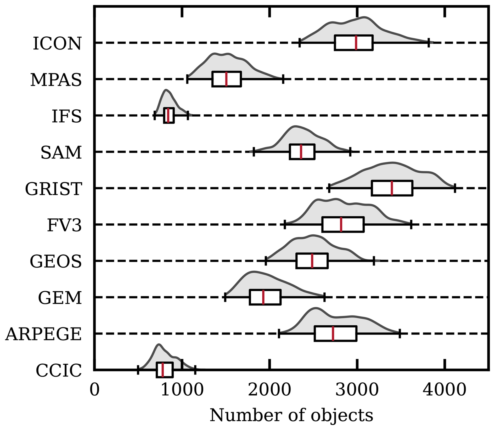
Figure 13 Distribution of number of convective core objects, inside 20° S to 20° N for each GSRM model and CCIC (February 2020). The grey areas are the probability distributions of object numbers, between model and retrieval time steps. A corresponding box-plot (representing the 0th and 100th percentile as whiskers, the 25th, 50 and 75th percentile as a box and the median as a red line) is shown underneath. Objects are defined as the set of adjacent grid cells (including diagonals) whose FWP value is in the top 3 % for the dataset of concern.

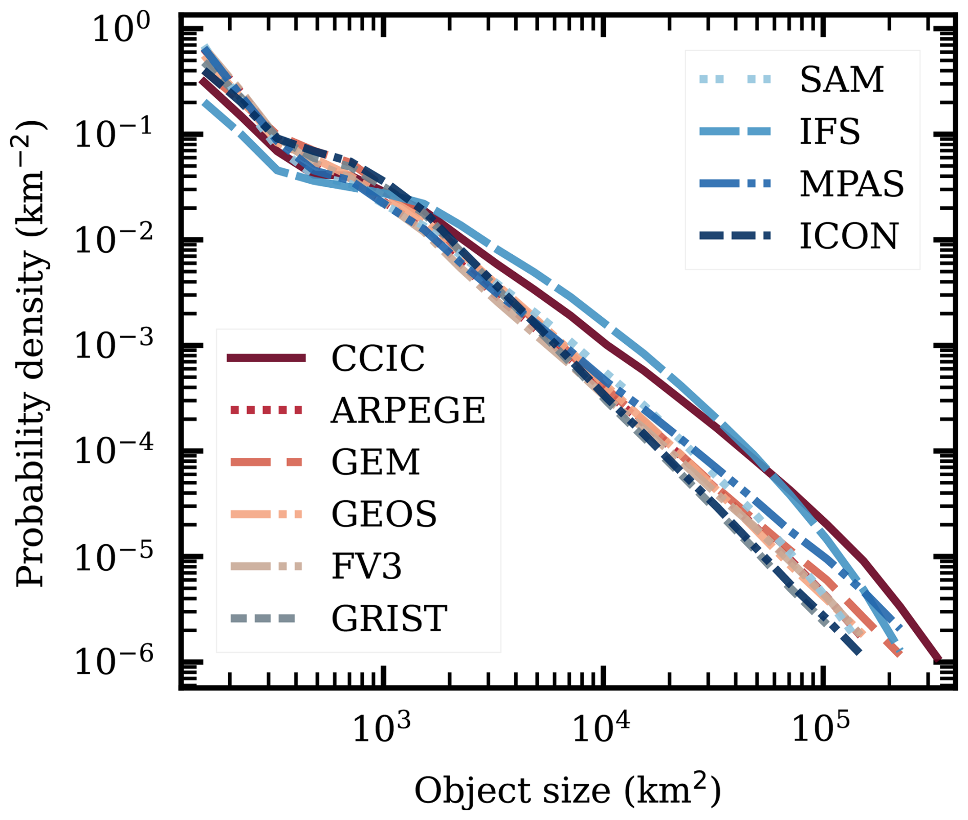
Figure 14 The probability distribution of convective core object areas. Considered area and definition of objects as in Fig. 13.

Figures 13 and 14 provide statistics of convective objects defined according to CC_n, i.e. as depicted by the highest fraction of FWP of each dataset. The strength of CCIC here emerges, since it is the only satellite-derived dataset providing the spatial coverage needed for this analysis. However, we remind about the limited horizontal resolution of CCIC, which can be seen in Fig. 1. CCIC should be reliable at large scales, but can be expected to underestimate the number of objects below about 10³ km².

The models exhibit a significant spread in the number of objects at each time step (Fig. 13), from means around 800 (IFS) up to 3500 (GRIST). CCIC, due to its limited resolution, is likely biased towards a small number of objects. In the small size range (Fig. 14), IFS is below CCIC, and this model is likely underestimating more localised areas of high FWP. At larger scales, e.g., for mesoscale convective systems, CCIC's resolution is of less concern. In the regime above 10⁴ km², we find that IFS has the best representation among all DYAMOND models. All other models have a considerably low bias compared to CCIC.

The diurnal variation of CC_n is found in Fig. 15. Land and sea have been separated by distinct cycles, with differences in both amplitude and peak times. According to CCIC, the amplitude is the highest over land, with a clear maximum in the late afternoon, while the less pronounced diurnal cycle over sea peaks around midnight. These patterns of CC_n are corroborated by most of the GSRMs. Again, IFS stands out, with close agreement with CCIC on both land and sea. Some models deviate from these patterns, in particular GEM. However, the overall impression of Fig. 15 is that GSRMs show promise in capturing features associated with convective diurnal variability, a known troublesome point for GCMs (e.g. Pritchard and Somerville, 2009). After assessing diurnal cycles of precipitation in different model types, Song et al. (2024) reached the same conclusion.

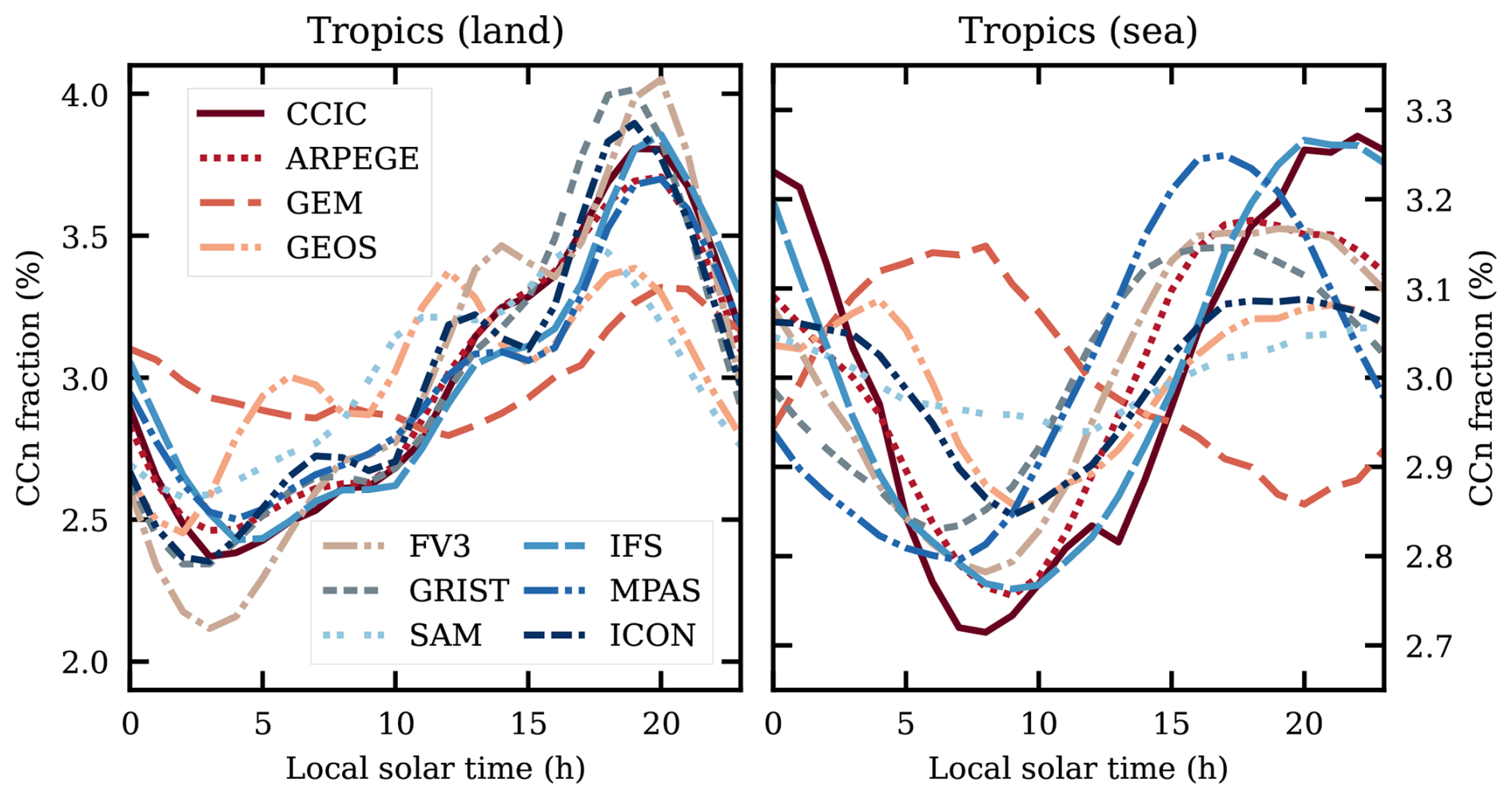
Figure 15 The diurnal variation of data exceeding the CC_n threshold, of the GSRM models and CCIC (February 2020), over land (left) and sea (right). The diurnal average of all datasets is 3 %, as stipulated by the definition of CC_n.

5.3 Convective organization indices

There is a growing interest in studying the organization and aggregation of convection in models and observations. To quantify and compare the organization of convection across different scenarios, numerous so-called organizational indices have been defined to measure the level of organization. However, at this time, there is no consensus on such an index. Mandorli and Stubenrauch (2024) reviewed and compared a number of such measures. Here, we apply seven of those indices to the GSRM data. The exercise is primarily a practical test to provide additional information on the behaviour of the DYAMOND models, rather than to establish a best index. Results for CCIC are provided, but its limited ability to resolve smaller high-FWP areas decreases its value as a reference, to varying degrees across the indices. Derived values are found in Table 8. Note that we modify the characteristic length scales used in Mandorli and Stubenrauch (2024) to allow for rectangular domains.

Table 8 Organization of convection according to seven measures. The results cover nine GSRMs and the CCIC satellite retrievals. Lowest and highest values among the models are marked as bold. Considered area and definition of objects as in Fig. 13.

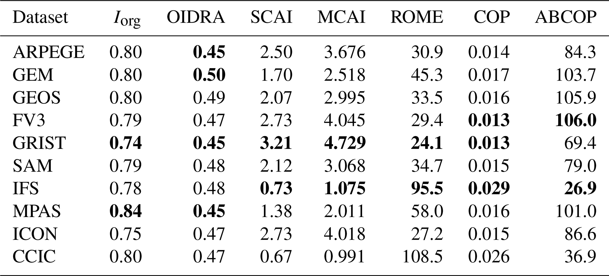
The first index, I_org, is based solely on the distances between convective objects. It classifies the spatial organization of convective areas as random (I_org=0.5), clustered (I_org>0.5), or regular (I_org<0.5). According to these categories the deep convection is clearly classified as clustered in all the GSRMs as well as in CCIC. The I_org index finds a similar level of clustering across in most datasets with I_org≈0.8. GRIST and ICON exhibit less clustered convection, while MPAS shows the strongest clustering. Using GridSat brightness temperature (T_b), Bony et al. (2020) reported an I_org=0.82 over tropical latitudes (±30° N). Despite analysing a different period (1990–2017) and using a different variable (T_b) and criterion to identify deep convective areas (defined as regions with T_b<240 K), their reported value falls within the range of our results – higher than the I_org for CCIC, yet still lower than that for MPAS (I_org=0.84).

The OIDRA index increases when convective objects are larger relative to the total convective area. It decreases as the distances between these objects increase. OIDRA is always smaller than 1 (Mandorli and Stubenrauch, 2024); lower values indicate reduced convective aggregation. For all GSRMs as well as CCIC, OIDRA identifies similar level of aggregation. It ranks GEM as the model with the highest, and MPAS as the one with the lowest, convective aggregation.

The SCAI and MCAI indices are based on the distances between objects, while MCAI additionally accounts for their size. Note that both indices reach maximum organization at zero; their lower bound. Mandorli and Stubenrauch (2024) shows that both indices strongly correlate with the number of convective objects. Our results reflect these findings (cf. Fig. 13). Accordingly, CCIC shows the strongest convective aggregation, with IFS in closest agreement among the GSRMs. Conversely, GRIST exhibits the weakest aggregation according to both indices.

The ROME index depends on the spatial proximity and size distribution of convective objects. Higher values indicate a greater degree of aggregation. In our data, ROME identifies IFS as the model with the strongest aggregation apart from the CCIC retrievals. On the other end, ICON exhibits the lowest aggregation. This ranking is consistent with Fig. 14, which reports much a higher number of large convective objects in CCIC and IFS compared to the other GSRMs. As such, our data supports the strong positive correlation with the objects mean size found in Mandorli and Stubenrauch (2024).

The COP index increases with the proximity and size of convective areas, with higher values indicating greater convective aggregation. However, Mandorli and Stubenrauch (2024) show that COP is not strongly correlated with the number, total area or mean size of the convective objects. According to this index, the convection in CCIC is more aggregated than in any of the GSRMs. Among the models, IFS exhibits the highest degree of convective aggregation and the closest agreement to CCIC, while GRIST and FV3 show the lowest levels aggregation.

Lastly, the ABCOP index is a modification of COP that has a strong correlation with the total area of convection over the studied domain (Mandorli and Stubenrauch, 2024). This index also reports IFS as the model that better agrees with CCIC, but also reports both of them as exhibiting lower aggregated convection than the rest of the models, in contrast with ROME, SCAI, MCAI and even COP.

The level of convective aggregation, and thus the ranking of the GSRMs, depends on the chosen index and the trust placed in the corresponding value derived from CCIC. SCAI, MCAI, ROME, and ABCOP consistently identify IFS as the closest match to CCIC in terms of convective aggregation. These indices exhibit strong correlation with the number and/or size of convective areas (Mandorli and Stubenrauch, 2024). As such, the results may be explained through Figs. 13 and 14. The three remaining indices, COP, I_org, and OIDRA, all correlate only weakly with the aforementioned variables. While COP also identifies IFS as the closest match to CCIC, I_org and OIDRA favour other models. In summary, all convective indices indicate that the models disagree about the level of convective organisation (using FWP as a proxy), but it is not possible to identify a best model due to the uncertainties in the reference values (derived from CCIC).

6 Conclusions

Accurately representing atmospheric ice remains a major challenge for climate science, as remaining limitations critically influence radiative transfer, vertical water transport, precipitation processes, and high-cloud radiative feedback. This study examined the representation of atmospheric ice mass in various types of circulation models and satellite observations, with the frozen water path (FWP) as a common benchmark. The conclusions refer to “all-weather” FWP averages; in-cloud means were not considered.

Global and zonal FWP means of considered CloudSat-based satellite retrievals (2C-ICE, DARDAR, and AOP) are within ±10 % and ±15 %, respectively (Sect. 3.4). This is a small spread compared to the poor agreement found in comparisons involving passive datasets (e.g. Duncan and Eriksson, 2018). However, these radar-based datasets can still exhibit both shared and counteracting biases, and systematic errors of the order of 30 %, with respect to a common best estimate, cannot be ruled out (Sect. 3.6).

Global climate models remain biased low. Most CMIP6 and HighResMIP models substantially underestimate FWPs compared to satellite-based estimates, particularly in the tropics. The overall spread among models is reduced compared to earlier generations; however, the systematic bias persists. One could think that the underestimation was due to models not reporting all forms of ice in their output; in particular, many models do not include precipitating ice. However, Fig. 5 shows that those models that do include precipitating ice in their output do not have systematically higher FWP compared to those that do not.

GSRMs represent a significant step forward. They capture a more comprehensive hydrometeor spectrum and represent deep convection explicitly, resulting in more realistic FWP distributions. Although significant differences remain when compared to observations, particularly for extreme events and regional variability, they are in a relatively early stage of development and there is hope for further progress within this new modelling paradigm in the near future.

No consensus “truth” exists. Both observations and models suffer from inherent limitations, leaving open the question of the true global distribution of atmospheric ice. This hinders the closure of the atmospheric water cycle and the quantification of associated radiative effects. This remark includes the fractioning between cloud ice, graupel, and snow; neither observations nor models provide a basis for distinguishing between the hydrometeor categories.

Future progress requires coordinated efforts. Advances in satellite missions (e.g., EarthCARE and ICI) and retrieval methodologies are essential. Cross-comparisons of independent datasets will be crucial in reducing uncertainties. Such comparisons should not only consider the value presented as the best estimate, but also whether the stated uncertainties are reasonable. To facilitate this, retrieval datasets shall make a clear separation between random and systematic errors, in line with the ambition level observed in other atmospheric satellite measurements (von Clarmann et al., 2020). Machine learning unlocks new possibilities, but, at least presently, constitutes a step backwards with respect to error characterisation; most such retrievals provide only broad, overall uncertainties, while cloud retrieval errors tend to be highly case-specific.

For GSRMs, there should be efforts to pinpoint the sources of the ice mass disagreement. Microphysics schemes are a possible source, but other parametrisations are also relevant. Although GSRMs lack some of the problematic parametrisations of GCMs (convective parametrisation, cloud scheme), others remain, in particular the turbulence scheme, which was identified by Lang et al. (2023) as a major source of discrepancies in the representation of the moisture distribution.

To facilitate comparison with satellite retrievals, we recommend to extend the saved output from atmospheric models. In the case of GCMs, the first step would be to report complete ice mass (including all forms of precipitating ice) at all, with adding FWP as the initial step. This quantity is already covered in publicly available GSRM datasets, and the natural continuation is also to provide vertically resolved data. On this side, we recommend starting with the total mass, i.e., frozen water content (FWC), if data volumes make it impractical to keep cloud ice, snow, and graupel contents separated.

Another way forward on the model side is to move away from a separation of distinct ice hydrometeor types and instead use a single-category model, such as the P3 scheme of Morrison and Milbrandt (2015). Interestingly, there are clear resemblances to P3 in the ice hydrometeor model used for the ACM_CAP EarthCARE product (Mason et al., 2023). Taken together, this gives hope for a more unified description of ice hydrometeors across models and observations.

In summary, while significant progress was made since earlier assessments, atmospheric ice mass remains to be much less well constrained than other atmospheric variables. Narrowing the uncertainties around FWPs is crucial for improving confidence in climate projections, because it would help us better constrain high cloud radiative feedbacks.

Appendix A: AOP radar inversions

This appendix complements Sect. 2.1.2 in the description of the ARTS onion peeling (AOP) algorithm. These radar inversions make use of pre-calculated look-up tables. The inversions are performed one layer at a time, beginning at the top of the atmosphere. The measured reflectivity in each layer is converted to an unattenuated reflectivity using the estimate of the two-way attenuation through the layer above. With the corrected value at hand, the local FWC and attenuation due to ice hydrometeors are derived from the look-up table matching the assumed particle habit and size distribution. The attenuation due to gases (nitrogen, oxygen and water vapour) is always considered. To include liquid water content (LWC) in the attenuation is optional. When considered, the microwave absorption of LWC is calculated following Ellison (2007). Amounts of water vapour and LWC are extracted from ERA5. The extinction of ice hydrometeors is included in all calculations in this study. However, AOP allows a rough scaling of this extinction to compensate for multiple scattering, based on results in Battaglia et al. (2010). In this work, the scaling factor is set to 0.5. If the attenuation in one layer is overestimated, it tends to result in a too high ice hydrometeor attenuation in lower layers as well. To avoid a runaway effect, the attenuation correction is not allowed to exceed 4 dB. As an additional measure, FWC is clipped at $\mathrm{5}\times {\mathrm{10}}^{-\mathrm{3}}$ kg m⁻³. In the absence of a comprehensive database of scattering data for oriented particles, look-up tables are generated based on data for totally random particle orientation. The effect of particle orientation is instead included as a term subtracted from measured reflectivities, specified in dB.

Appendix B: Time series and trends of GCM FWPs

Time-series of monthly global mean FWP are shown in Fig. B1. Local changes in mean FWP are displayed in Figs. B2 and B3, as relative trends with respect to the local mean FWP over the time period considered.

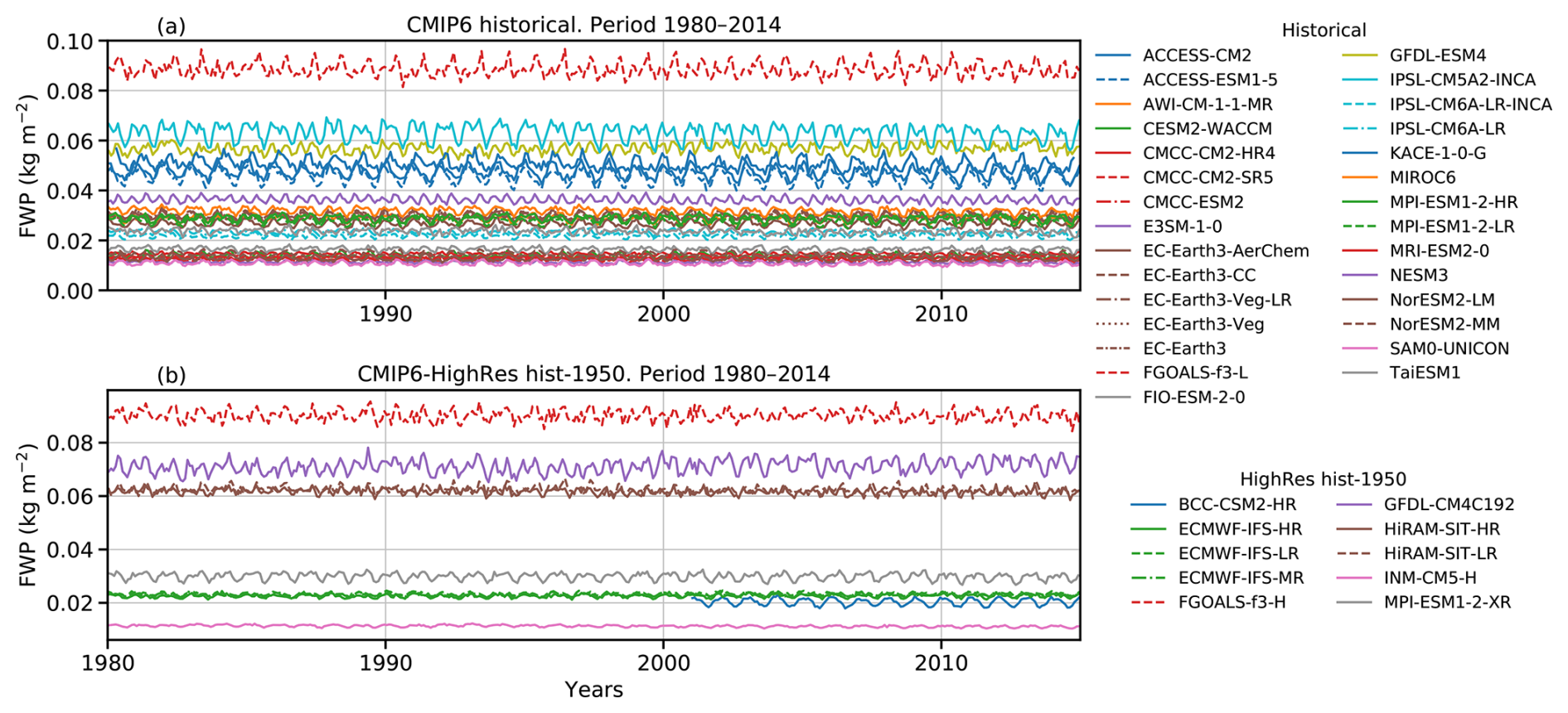
Figure B1 Time series of monthly means FWP between 60° S and 60° N during the period 1980–2014 for (a) CMIP6 historical simulations, and (b) CMIP6 HighRes hist-1950 simulations.

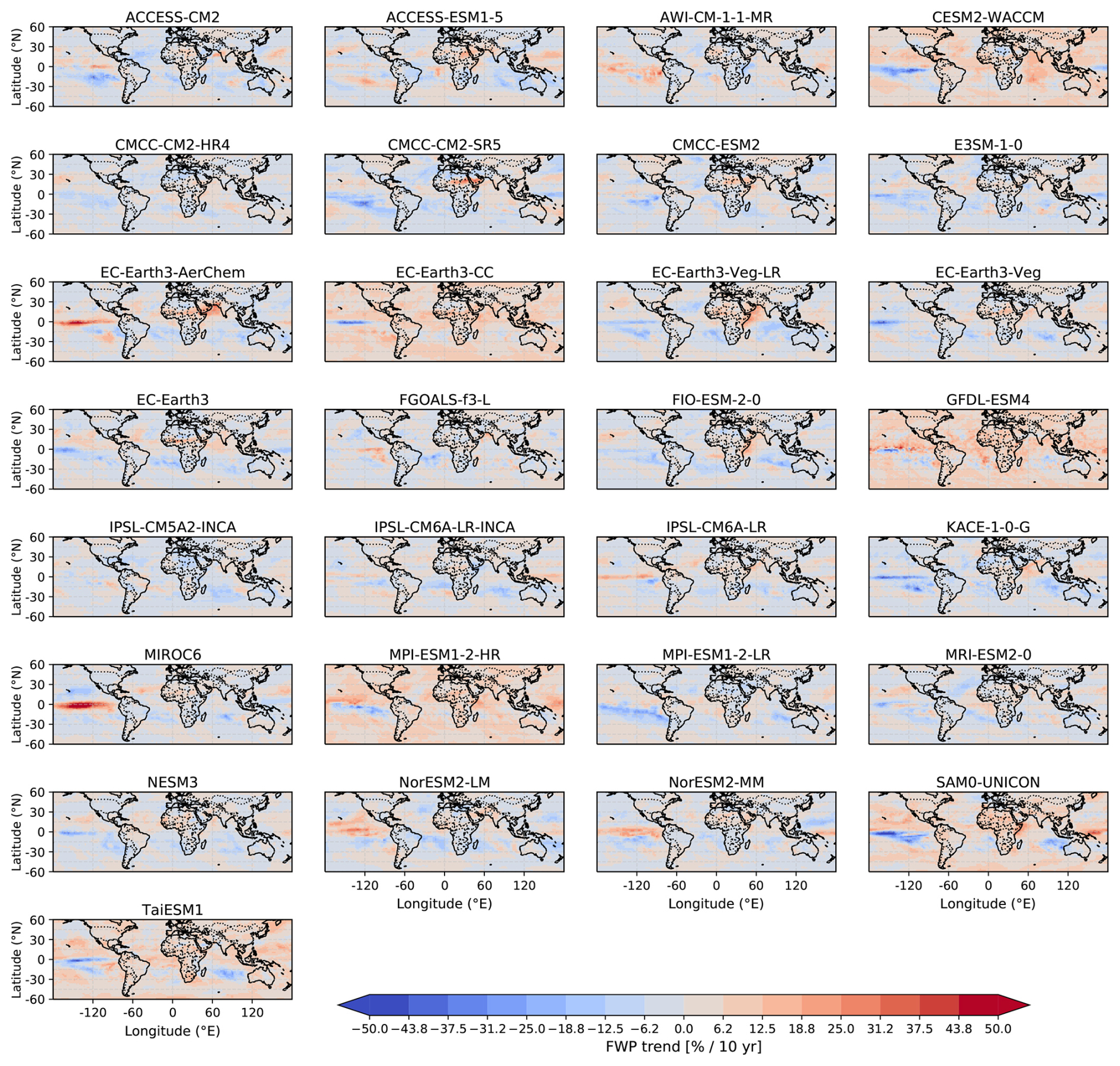
Figure B2 Decadal FWP trends from 1980 to 2014 for the CMIP6 historical simulations. The trends based on the monthly mean values in each model grid cell for the full period. Red-shaded regions correspond to increases in FWP, whereas blue-shaded regions correspond to decreases in FWP.

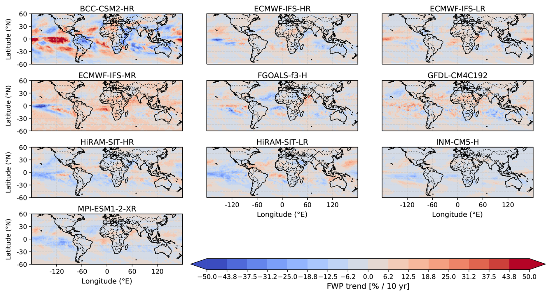
Figure B3 Decadal FWP trends from 1980 to 2014 for the CMIP6 HighRes hist-1950 simulations. Red-shaded regions correspond to increases in FWP, whereas blue-shaded regions correspond to decreases in FWP.