Constraining a data-driven CO₂ flux model by ecosystem and atmospheric observations using atmospheric transport

Global estimates of the net ecosystem exchange of CO₂ (NEE) from data-driven models differ widely depending on their underlying data and methodology. Bottom-up models trained on eddy-covariance data are most informative at the ecosystem-level. Top-down models, such as atmospheric inversions, produce regional and global results consistent with the observed atmospheric growth rate, accurately capturing the interannual variability (IAV) of NEE. Both approaches have limitations estimating NEE across scales: Bottom-up models can miss large-scale dynamics of NEE when aggregated globally. Top-down approaches have difficulty relating the large-scale atmospheric signal to biophysical processes at smaller scales. To address these limitations, we create a model that uses a hybrid combination of direct observations and atmospheric dynamics to integrate ecosystem-level eddy-covariance data and atmospheric CO₂ mole fraction data into a single coherent ecosystem-level flux model.

Aggregated globally, our new model estimates an annual sink with a low bias, and consistent IAV when compared with independent estimates. The IAV of the estimated NEE is closer in magnitude to an ensemble of atmospheric inversions, and our model produces a higher temporal coefficient of correlation with these data than state-of-the-art bottom-up data-driven models. This improvement in IAV is achieved without direct access to the observed variability of the atmosphere: the model is trained using only one year of daytime observations from 3 tall-tower observatories. No atmospheric information is available to the model during the production of global NEE estimates. This shows the efficiency of our method in synthesizing top-down information into bottom-up mapping of flux-environment relationships.

1 Introduction

The global net flux of biogenic CO₂ between the land surface and the atmosphere, or net ecosystem exchange (NEE), is a critical but uncertain term in our understanding of the global carbon budget and the climate system (Friedlingstein et al., 2014; Bastos et al., 2022). Current data-driven approaches to modeling NEE can be largely grouped into two categories: top-down approaches that infer NEE from observations of atmospheric CO₂ by prescribing fire and fossil fuel emissions. The second category are bottom-up approaches that model NEE at the ecosystem level from local observations (Kondo et al., 2020). Both approaches provide important information about the function of the biosphere, but have their limitations.

Data-driven bottom-up models are most commonly informed by eddy-covariance observations at the ecosystem scale, along with remotely sensed variables (greenness and water indices, spectral data) (Nelson and Walther et al., 2024; Jung et al., 2020; Kondo et al., 2020; Bodesheim et al., 2018). However, the spatial distribution of NEE and the total magnitude of NEE at global scale remain highly uncertain as the available eddy-covariance data is sparse in important biomes across the globe, such as tropical rain forests (Chu et al., 2017; Hayek et al., 2018; Fu et al., 2018; Jung et al., 2020). Some processes, such as carbon emissions from fires, are not captured by these local observations. Eddy-covariance data are further potentially subject to systematic errors overestimating the carbon uptake (Aubinet et al., 2005), particularly in the tropics, due to complex CO₂ nighttime storage and horizontal advection in the canopy (Fu et al., 2018; Moncrieff et al., 1996). Historically, when these eddy-covariance data are used to train a data-driven bottom-up flux model for global upscaling of NEE (e.g. FLUXCOM V1, Jung et al., 2020), the underlying issues of data availability and representation are propagated into the global result resulting in an overestimation of the tropical carbon sink and by extension, the global carbon sink. Therefore data-driven global products such as FLUXCOM V1 NEE, which are very dependent on the quality and completeness of the training data, are not fully consistent with the magnitude of the growth rate of atmospheric CO₂, or the interannual variability (IAV) of the global NEE signal (Jung et al., 2020; Kondo et al., 2015). However the length of the available eddy-covariance record has increased, and the data collection and processing have improved (Pastorello et al., 2020). These longer, improved data, along with improved handling and gap-filling of the complementary co-located remotely sensed variables (Walther and Besnard et al., 2022) have allowed for FLUXCOM X-BASE to improve its estimates of the magnitude of regional and global NEE. Despite these improvements, the eddy-covariance record may miss complex drivers of IAV, or they may be obscured by sensor issues (Jung et al., 2024). The under-estimation of the global NEE IAV in FLUXCOM X-BASE remains unresolved (Nelson and Walther et al., 2024).

Top-down approaches, most commonly atmospheric inversions, are trained using observations of CO₂ mole fraction from tall-tower observatories and/or satellite retrievals of CO₂. Atmospheric inversions use a Bayesian inversion framework and an atmospheric transport model to produce global or regional estimates of NEE which are consistent with the observed atmospheric signal (Chevallier et al., 2005; Peylin et al., 2013; Crisp et al., 2022; Ciais et al., 2022). These inversion systems by design provide estimates of NEE that agree with the growth rate of CO₂ at the global scale and across broad latitudinal bands (Peylin et al., 2013) despite differences in priors and representation of transport mechanisms. Atmospheric inversions are formulated to capture the structure and dynamics of atmospheric CO₂, and can reproduce the observed IAV of NEE with very high accuracy (Rödenbeck et al., 2018).

However, despite improvements in the ability of regional inversions to provide spatially explicit flux estimates (Munassar et al., 2022), global top-down estimates of NEE lack the ability to spatially map the atmospheric signal to local biophysical conditions. Global inversions are more commonly used to understand the land surface at larger integrated scales, and are not directly comparable with eddy-covariance data (Kaminski and Heimann, 2001). Like bottom-up systems, the top-down approach is also limited by a lack of observations. The observational network does not provide sufficient tropical coverage for a robust top-down estimate of the tropical land flux (Palmer et al., 2019). In the Southern Hemisphere, the weaker gradients in CO₂, and shorter observational records also exacerbate issues of data availability and data quality (Peylin et al., 2013). Additionally, in tropical regions there are less independent data to validate atmospheric inversion estimates (Chevallier et al., 2019).

Previous work has demonstrated that top-down information can be effectively combined with a bottom-up data-driven flux model, improving the regional and global performance by creating a dual constraint from eddy-covariance data and atmospheric inversion estimates of NEE (Upton et al., 2024). Although this dual-constrained model was able to infer regional and global NEE integrals with a much lower bias compared with other best estimates of NEE than the comparable FLUXCOM RS+METEO V1 results (Jung et al., 2020), the model has several important limitations; First, the atmospheric constraints were pre-calculated using large-scale mean NEE from an ensemble of inversions, rather than from atmospheric CO₂ itself. Second, the atmospheric constraint was connected to the local bottom-up data-driven flux model using a static, statistical model rather than an atmospheric transport model. This means that the additional atmospheric information is aggregated, and adds no additional information on the spatial distribution of NEE. Both issues limited the amount of information available to the model from the atmospheric constraint.

To address these limitations, we create a new model that uses a hybrid combination of direct observations and atmospheric dynamics to integrate ecosystem-level eddy-covariance data and atmospheric CO₂ mole fraction data into a single coherent ecosystem-level flux model. To create the computational link between ecosystem-level fluxes and atmospheric CO₂ mole fraction we use a physical atmospheric transport model, the Stochastic Time-Inverted Lagrangian Transport (STILT) model (Lin et al., 2003). In this way, both eddy-covariance and atmospheric observations are used to train and update the model at the ecosystem level, the result is a bottom-up model that uses atmospheric data to improve the representation of the land surface. This technique opens a large corpus of new observations for constraining the model. Due to varying transport patterns around each tower, the data-driven model is exposed to a large number of non-eddy-covariance locations which represent biophysical conditions that are coupled to important dynamics in global NEE. This enrichment of the model's view of the underlying relation between driver variables and NEE, we hypothesize, allows the system to learn additional dynamics in global, and regional NEE.

2 Data

2.1 Ecosystem-level data

At the ecosystem level, we define Net Ecosystem Exchange (NEE) as the simple difference between Gross Primary Production (GPP) and Total Ecosystem Respiration (TER). These terms are measured as the flux density $\mathrm{\mu }\mathrm{mol}{\mathrm{CO}}_{\mathrm{2}}{\mathrm{m}}^{-\mathrm{2}}{\mathrm{s}}^{-\mathrm{1}}$. The sign of NEE indicates the direction of the flux. When NEE is negative, GPP exceeds TER and the flux is a local sink of CO₂. If NEE is positive, TER exceeds GPP and the ecosystem is a local source. NEE represents the net carbon exchange of the vegetation and does not include disturbance fluxes, fires, or out-gassing from freshwater ecosystems.

The core ecosystem-level meteorological and NEE data was collected between 2001 and 2020 at 294 globally distributed eddy-covariance (EC) towers (see appendix for a full list of sites). These data were then processed using the ONEFLUX processing pipeline (Pastorello et al., 2020). Variables from the eddy-covariance sites are air temperature, vapor pressure deficit, incoming shortwave radiation, the computed potential shortwave incoming radiation, and the computed wind speed.

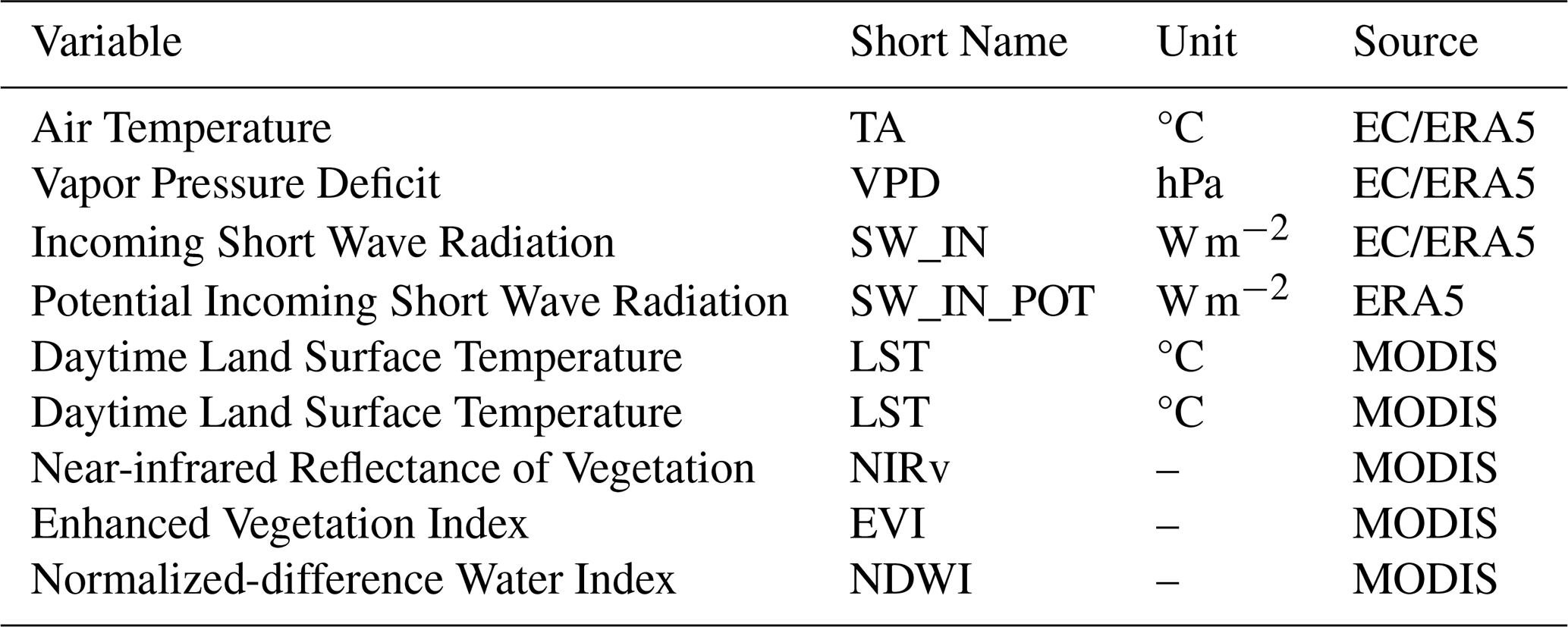
During training, at pixels co-located with eddy-covariance towers we use the surface reflectances (MCD43A4, Schaaf and Wang, 2015a) and land surface temperature (LST) from the MOderate Resolution Imaging Spectroradiometer (MODIS) collection v006 (http://daac.ornl.gov/MODIS/, last access: 11 January 2024). The surface reflectances are used to compute two vegetation indices, the enhanced vegetation index (EVI) (Huete et al., 2002), and the spectral reflectance of vegetation in the near-infrared (NIRv) (Badgley et al., 2019). A water index, the normalized difference water index (NDWI) with MODIS band 7 (Gao, 1996) was also included. MODIS data has a spatial resolution of 0.05°, and a 1 d temporal resolution. The full set of variables is described in Table 1.

Table 1 Driver variables for the model (EC-STILT) in this study.

When producing our atmospheric constraint, and when estimating global NEE, the drivers for our bottom-up model are the same set of remotely-sensed and eddy-covariance quantities, extracted from remotely-sensed and meteorological reanalysis data. The RS data are derived from the 0.05° global MODIS product (MCD43C4, Schaaf and Wang, 2015b), and the global meteorological variables are derived from the European Center for Medium-Range Weather Forecasting (ERA5) atmospheric reanalysis data (https://www.ecmwf.int/en/forecasts/dataset/ecmwf-reanalysis-v5, last access: 11 January 2024). ERA5 is provided at 0.25° spatial resolution, and hourly temporal resolution (Hersbach et al., 2020). Air temperature at 2 m height, incoming shortwave radiation, and vapor pressure deficit (computed from air temperature, relative humidity, and surface pressure) are used to create the global meteorological data.

All data are accessed through the FLUXCOM-X code base using the preprocessing, and gap-filling from Nelson and Walther et al. (2024) and the procedures of FluxnetEO data version 2 (Walther and Besnard et al., 2022), and the quality flagging described in Jung et al. (2024). Please see Nelson and Walther et al. (2024) for a full description of the FLUXCOM-X data and processing environment.

2.2 Atmospheric data

The model in this study uses observations of atmospheric CO₂ mole fraction from tall-tower observatories measured at three sites: ATTO (Botia et al., 2022), Hegyhatsal (Haszpra, 2024) and Zottino (Tran et al., 2024a). These sites are chosen to include one tropical, one extra-tropical and one boreal domain. The mole fraction data used for the Amazon Tall Tower Observatory in Brazil (ATTO), collected at 79 m are the same used and fully described in Botia et al. (2022). Mole fraction data for the Hegyhátsál tower in Hungary (HUN), collected at 115 m are provided by the Integrated Carbon Observation System (ICOS). The observations for the Zotino Tall Tower Observatory in Siberia (ZOTTO), collected at 301 m are provided by Tran et al. (2024b). The data for all three towers was provided hourly, for one calendar year (2019 for ZOTTO and Hegyhátsál, 2015 for ATTO). Only daytime observations from 13:00–17:00 (local time) were used. The selected times represent a daytime planetary boundary layer (PBL) with assumed well-mixed convective conditions (Peters et al., 2010).

2.3 Reference data

For global and regional comparison we use the land flux corrected for fossil fuel and cement production from the ensemble of N=14 atmospheric inversions from GCB23 (https://doi.org/10.18160/4M52-VCRU, Luijkx et al., 2024, last access: 4 March 2024). The atmospheric inversions are provided as monthly data with a 1° spatial resolution. See Friedlingstein et al. (2023) for a full description of the ensemble members. These fluxes are adjusted for fire by removing the fire emissions from Global Fire Emissions Database, Version 4.1 (GFEDv4) (last access: 13 February 2024) (Randerson et al., 2017).

For comparison with the current state-of-the-art bottom-up NEE model, we use the global NEE product from the latest version of FLUXCOM X-BASE (Nelson and Walther et al., 2024, last access: January 2025). The FLUXCOM X-BASE NEE model (hereafter X-BASE) is trained using the same data processing and data quality flagging, including gap-filling. X-BASE uses a different data-driven algorithm, XGBoost (Chen and Guestrin, 2016), instead of a neural network. Comparison with X-BASE allows us to understand the performance of our system relative to a highly optimized bottom-up model. So, despite differences in structure, we consider X-BASE to be the most appropriate bottom-up model for comparison.

For regional analysis we use the set of 11 large regions from the TransCom 3 intercomparison project (TransCom) project (Baker et al., 2006). See Fig. A1 for the coverage and names of the 11 land regions used in this study. For analysis of model function by climate zone, we use the Köppen-Geiger (KG) classification system using maps from Beck et al. (2018), for the years 1991–2020. The Köppen-Geiger classification groups the land-surface into regions by their annual climate (Fig. A2).

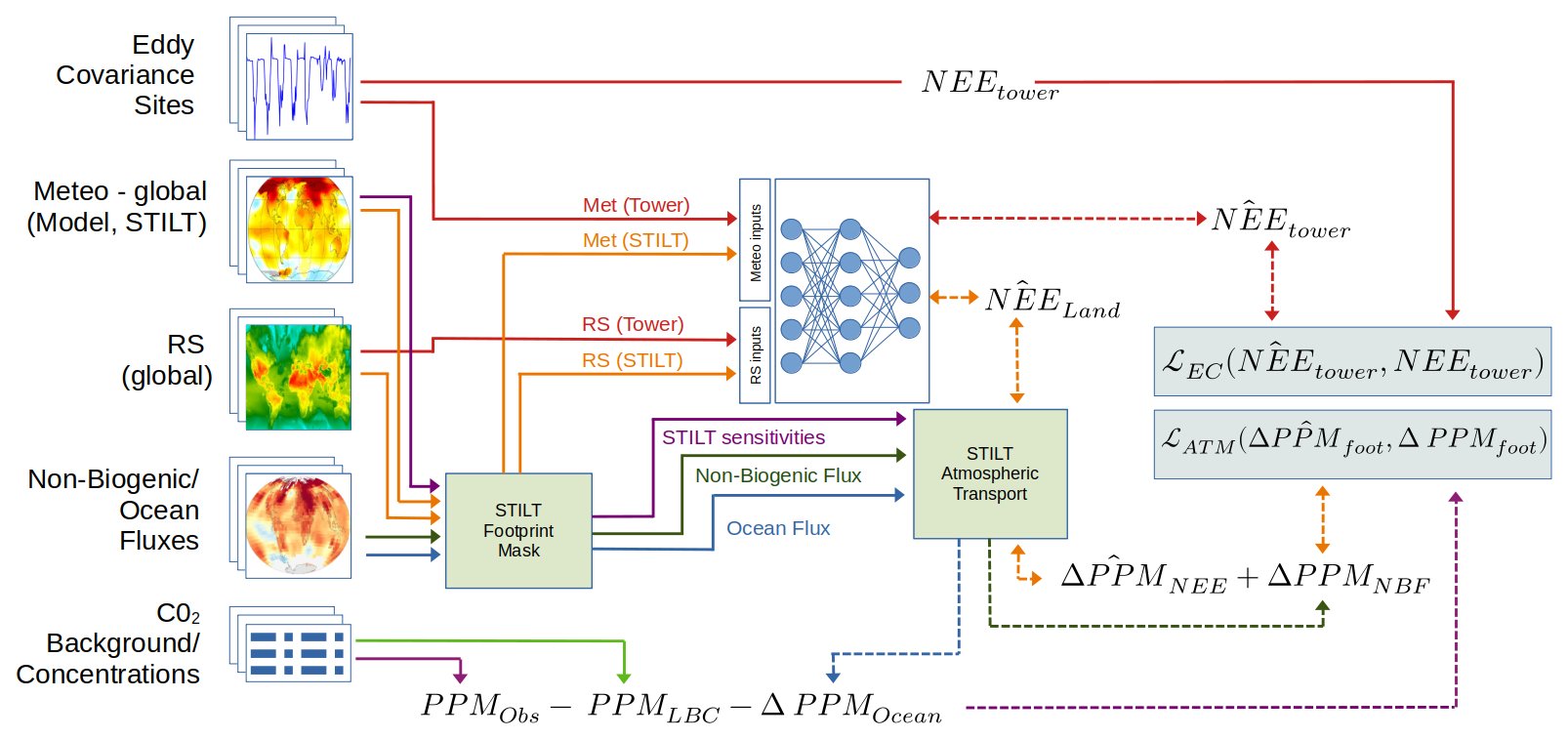
Figure 1 Data flow for atmospheric constraint calculation. An objective term from eddy-covariance (red lines) is created from tower observations of driver variables, co-located remotely sensed data, and tower observations of NEE. An objective term from atmospheric observations (model: orange lines, ancillary data: other colors) uses the STILT model to transport modeled flux densities into concentration space, and corrected for non-local and non-biogenic CO₂: The lateral boundary condition (PPM_LBC), or background CO₂ from the well-mixed atmosphere, and any ocean flux contributions (ΔPPM_Ocean) are removed from the tower observation (PPM_Obs) to create the observed value for the contribution from the footprint (ΔPPM_foot). Non-biogenic fluxes (ΔPPM_NBF) from fire and fossil fuels are added to the predicted NEE from the footprint ($\mathrm{\Delta }{\widehat{\text{PPM}}}_{\mathrm{NEE}}$) to produce the predicted contribution from the footprint ($\mathrm{\Delta }{\widehat{\text{PPM}}}_{\mathrm{foot}}$). Dashed lines indicate terms that are created during the process of training. See Sect. 3.3 and 3.4 for a full description of terms. Lines with bi-directional arrows indicate the flow of backpropagation leading to the weights of the neural network being updated.

3 Methods

In this work, we start with a neural network model which uses eddy-covariance, meteorological, and remotely sensed data to estimate NEE at the ecosystem level. We create a hybrid objective function which allows direct constraint by eddy-covariance (EC) observations and hybrid constraint from direct mixing ratio observations of CO₂ using the Stochastic Time-Inverted Lagrangian Transport (STILT) atmospheric transport model as the computational link from the EC-model to the top-down observations. We therefore refer to this new data-driven system with its dual constraints as EC-STILT. Its components and their recombination in a machine-learning framework are described below.

3.1 Ecosystem-level model

The ecosystem-level model takes as input observations of meteorological drivers (from eddy-covariance or reanalysis data) and remotely-sensed drivers and predicts NEE in $\mathrm{\mu }\mathrm{mol}{\mathrm{CO}}_{\mathrm{2}}{\mathrm{m}}^{-\mathrm{2}}{\mathrm{s}}^{-\mathrm{1}}$ (Fig. 1, red lines, orange lines) at an hourly tempo. As a machine-learning system, the ecosystem-level model can be described as a feed-forward neural network trained using standard backpropagation techniques (Kelley, 1960). The network is a set of fully-connected layers which consist of nodes or “neurons”. The neurons are exposed to the output of all neurons in the previous layer. Between each layer of neurons, the output is passed through a non-linear activation function. Additionally, the output of the activation function is passed through a normalization function, which scales the output to a mean of 0 and a standard deviation of 1. Our network is a set of three fully-connected layers with the Rectified Linear Unit (ReLU) activation function (Agarap, 2019) and batch normalization. Each layer in a neural network is a complex, non-linear embedding of the previous inputs into a new latent space. This series of embedding functions is the learning space of the network. These latent spaces allow the model to learn complex non-linear relationships between driver variables and NEE. Because these relationships are discovered in these abstract non-geographic spaces, they can represent complex space-for-time and time-for-space substitutions. We refer to the process of learning these non-linear, non-geographic mappings between the input distribution and NEE as learning in “environmental response” space.

3.2 STILT transport

The computational link from this ecosystem-level model to the atmospheric constraint (Fig. 1, purple lines) is built around the STILT atmospheric transport model (Lin et al., 2003). STILT is a Lagrangian particle dispersion model (LPDM) which uses meteorological forcing data to compute the transport of sources and sinks to the time and location of an observation. The STILT footprint represents this atmospheric transport as a set of sensitivities of the final observation to fluxes at different times and locations. This footprint can be multiplied with a set of local estimates of NEE, which transports them and converts them into a simulated mole fraction. EC-STILT uses a set of pre-computed STILT footprints at the three tall tower locations, for midday observations, for one year (Fig. 1). For each tower, the STILT model is run for each selected observation over the year, producing footprints covering the tower domain hourly for the 10 d prior to the observation time. STILT domains (Fig. 2) are selected to capture the relevant near field over the time of analysis based on regional meteorological conditions (Lin et al., 2003).

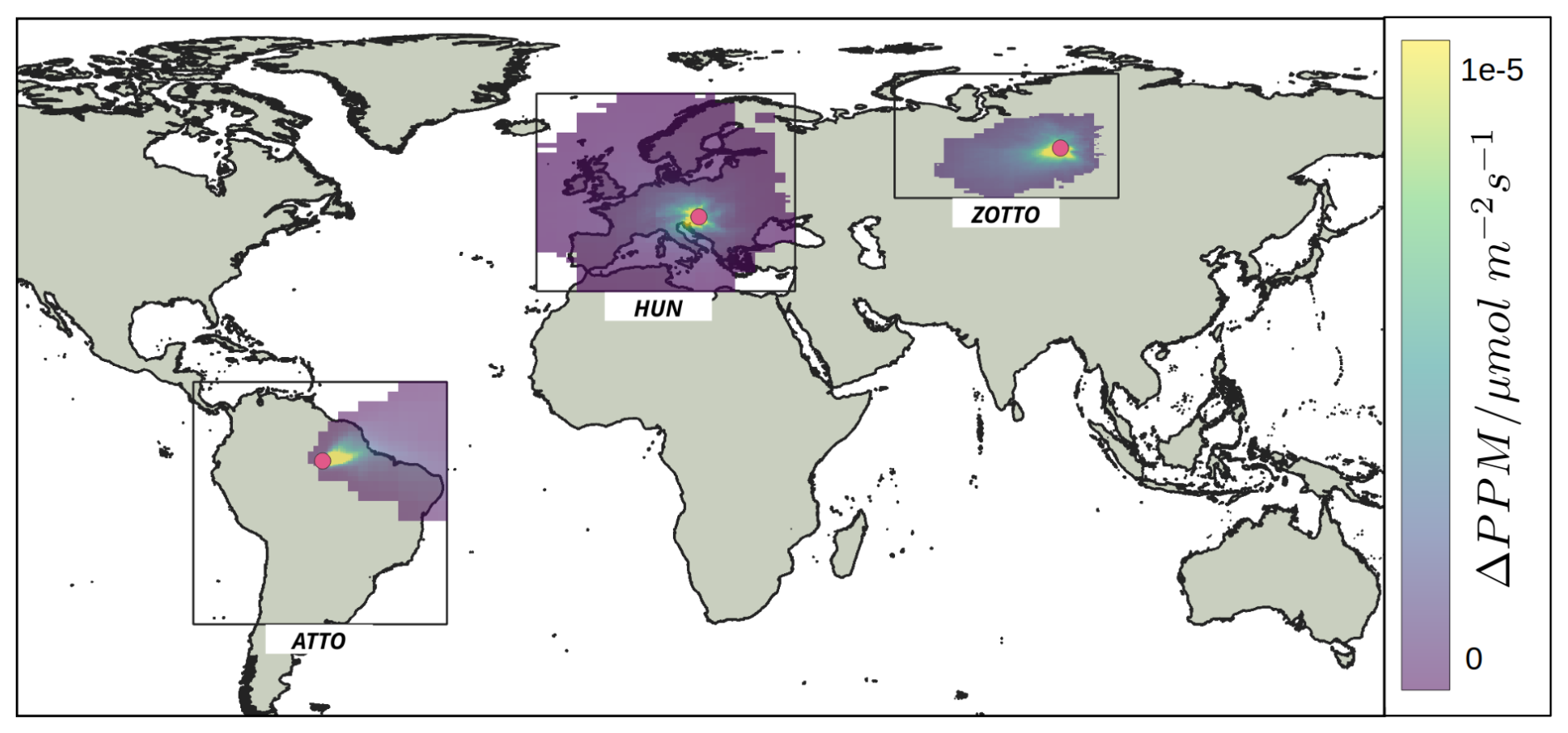
Figure 2 Locations of tall towers used by the atmospheric constraint (red dots). The boxes represent the near-field domain where STILT is computed, and the grid within each domain is the mean annual sensitivities of the computed STILT footprints. The colorbar, in $\mathrm{\Delta }\text{PPM}(\mathrm{\mu }\mathrm{mol}{\mathrm{m}}^{-\mathrm{2}}{\mathrm{s}}^{-\mathrm{1}}{)}^{-\mathrm{1}}$, represents the mean sensitivity of the tower observation to the region over the full year.

For the atmospheric constraint, we must isolate the biogenic contribution (ΔPPM_NEE) of an hourly observation of CO₂ (PPM_Obs). Conceptually, the biogenic contribution is the residual of the observation and the non-biogenic terms: the lateral boundary condition (LBC), non-biogenic fluxes (NBF) and Ocean contributions. This is presented in Eq. (1), with spatially explicit terms on the right.

$$\begin{array}{}\text{(1)}& {\mathrm{PPM}}_{\mathrm{Obs}}-{\mathrm{PPM}}_{\mathrm{LBC}}-\mathrm{\Delta }{\mathrm{PPM}}_{\mathrm{Ocean}}=\mathrm{\Delta }{\mathrm{PPM}}_{\mathrm{NEE}}+\mathrm{\Delta }{\mathrm{PPM}}_{\mathrm{NBF}}\end{array}$$

The NBF contribution (ΔPPM_NBF) consists of fossil fuel fluxes and fire emissions. For fossil fuel emissions, we use fossil fuel/energy signal across sectors, using GridFED (version 2022.2, last access: 15 February 2024) (Jones et al., 2021), provided at a 0.1° resolution. Fire emissions are provided by the Global Fire Emissions Database, Version 4.1 (GFEDv4) (last access: 13 February 2024) (Randerson et al., 2017) provided at a 0.25°. For the GFEDv4 data, temporal profiles were used to add monthly, daily, and diurnal cycles to the fire signal. The GridFED data are interpolated to the 0.25° spatial resolution of the analysis. We do not include lateral transport fluxes in the current analysis. Crop and wood harvest are important for regional and long term accounting (Ciais et al., 2022), but are not critical for the instantaneous carbon budget that is represented in Eq. (1). The potential impact of riverine transport are discussed below in Sect. 5.1.

The lateral boundary condition of the region (PPM_LBC) is precomputed using The Jena CarboScope (s04ocv4.3) (Rödenbeck et al., 2003), following Botia et al. (2022). Optimized results from the CarbonTracker Data Assimilation Shell (CTDAS) (van der Laan-Luijkx et al., 2017) (CTE2020) are used for the ocean flux and its conversion to mole fractions (ΔPPM_Ocean) with STILT. The LBC values are calculated for each tall tower for each observation time. We used the ensemble of STILT trajectories released at each data point to obtain the mean ending position (lat, lon) as well as a mean ending height above the ground. Using this information we sample global 3D fields, in this case the optimized CO₂ mole fractions from CarboScope, and obtain a mole fraction associated with a measurement at the tower. We acknowledge that this method is sensible to biases in the global 3D fields, but for example at ATTO a bias-corrected version of the LBC yielded very similar results to the CarboScope LBC, please see Botia et al. (2022) for the full discussion.

3.3 Objective function – eddy covariance

During training, EC-STILT generates an objective function with two terms, or losses: the ecosystem loss term ℒ_EC, and the atmospheric loss term ℒ_ATM. To generate the ecosystem loss term ℒ_EC from eddy-covariance, the EC-model ℱ() is run using a batch of data randomly selected by time and site, x_batch collected at eddy-covariance tower sites (Eq. 2, along with remotely sensed (RS) data at pixels that are co-located with the eddy-covariance tower, producing an estimate of NEE at the ecosystem level (Eq. 2). The ecosystem loss term is computed as the mean squared error (MSE) between this estimate and the observed NEE from the eddy-covariance observations (Eq. 3).

$$\begin{array}{}\text{(2)}& {\displaystyle }\widehat{\mathrm{NEE}}& {\displaystyle }=\mathcal{F}\left(x_{\mathrm{batch}}\right)\text{(3)}& {\displaystyle }{\mathcal{L}}_{\mathrm{EC}}& {\displaystyle }=\text{MSE}({\mathrm{NEE}}_{\mathrm{obs}},\widehat{{\mathrm{NEE}}_{\mathrm{tower}}})\end{array}$$

3.4 Objective function – atmospheric

To generate the atmospheric loss term ℒ_ATM for each training step, an hourly daytime (13:00 to 17:00 local time) observation of the mole fraction of CO₂ for each tower is selected. For each observation, a pre-computed STILT footprint, along with associated NBF, LBC and ocean data are retrieved. The observed mole fraction, LBC and ocean contributions are used to create the left-hand side of Eq. (1). The ocean term represents the flux from any pixels under the footprint, transported using the footprint into concentration enhancements at the tower. To create the right-hand side of Eq. (1), which is the change in CO₂ mole fractions attributable to fluxes within the footprint (ΔPPM_foot). The ecosystem-level model is then run for each non-zero location in the STILT footprint, producing an estimate of local NEE (Fig. 1, NEE_land). The NEE inferences and NBF values are transported with the footprint into concentration enhancements at the tower. This produces the two terms ΔPPM_NEE, and ΔPPM_NBF which are then added element-wise. These sums represent the total simulated change in PPM at the tower. The loss term ℒ_tower,ATM is the squared difference between the simulated change in concentration ${\widehat{\mathrm{\Delta }\text{PPM}}}_{\mathrm{foot}}$, and the observed change in concentration ΔPPM_foot. For a single training step, a loss is calculated for one observation for every tower. These three tower losses are averaged, producing the final atmospheric loss term (Eq. 5).

$$\begin{array}{}\text{(4)}& {\displaystyle }{\mathcal{L}}_{\mathrm{tower},\mathrm{ATM}}& {\displaystyle }=(\mathrm{\Delta }{\mathrm{PPM}}_{\mathrm{foot}}-{\widehat{\mathrm{\Delta }\text{PPM}}}_{\mathrm{foot}}{)}^{\mathrm{2}}\text{(5)}& {\displaystyle }{\mathcal{L}}_{\mathrm{ATM}}& {\displaystyle }={\displaystyle \frac{{\sum }_t^{\mathrm{Num}.\mathrm{Towers}}{\mathcal{L}}_{\mathrm{t},\mathrm{ATM}}}{\mathrm{Num}.\mathrm{Towers}}}\end{array}$$

The two terms of the objective function, ℒ_EC and ℒ_ATM are combined using a learned weighting scheme (Kendall et al., 2018). This allows the model to learn the appropriate relative weight to assign each loss term during training, based on their internally estimated uncertainty. To achieve this, the model has a set of additional parameters which are used to learn an estimate of the homoscedastic uncertainty for each term of the objective function. This uncertainty is dependent on the inherent noise in the training data, rather than the quality or quantity of training data. For EC-STILT these mixing parameters, ${\mathit{\sigma }}_{\mathrm{EC}}^{\mathrm{2}}$ and ${\mathit{\sigma }}_{\mathrm{ATM}}^{\mathrm{2}}$, are added to the processing chain of the model after its initialization. During training, using the normal backpropagation process that uses the chain rule to attribute and update the free parameters of the neural network according to their contribution to the loss value, the model also updates these mixing parameters. For the individual tasks $L\in [\mathrm{EC},\mathrm{ATM}]$, the ${\mathit{\sigma }}_{\mathrm{L}}^{\mathrm{2}}$ parameter is used to create two terms; w_L (Eq. 6), and s_L (Eq. 7). These are then used to calculate the effective loss, balanced by the learned uncertainty of the terms (Eq. 8). The evolution of these terms during training is provided in Fig. A4. After this final weighting calculation, the loss is combined in small batches to stabilize model training during backpropagation.

$$\begin{array}{}\text{(6)}& {\displaystyle }{w}_{\mathrm{EC}}& {\displaystyle }={\displaystyle \frac{\mathrm{1}}{\mathrm{2}{\mathit{\sigma }}_{\mathrm{EC}}^{\mathrm{2}}}},w_{\mathrm{ATM}}={\displaystyle \frac{\mathrm{1}}{\mathrm{2}{\mathit{\sigma }}_{\mathrm{ATM}}^{\mathrm{2}}}}\text{(7)}& {\displaystyle }{s}_{\mathrm{EC}}& {\displaystyle }=\log \sqrt{{\mathit{\sigma }}_{\mathrm{EC}}^{\mathrm{2}}},s_{\mathrm{ATM}}=\log \sqrt{{\mathit{\sigma }}_{\mathrm{ATM}}^{\mathrm{2}}}\text{(8)}& {\displaystyle }{\mathcal{L}}_{\mathrm{total}}& {\displaystyle }=(w_{\mathrm{EC}}\times {\mathcal{L}}_{\mathrm{EC}})+(w_{\mathrm{ATM}}\times {\mathcal{L}}_{\mathrm{ATM}})+s_{\mathrm{EC}}+s_{\mathrm{ATM}}\end{array}$$

3.5 Model training

EC-STILT is trained using 10-fold cross-validation. The full set of eddy-covariance observations are split by tower location into 10 equal subsets. Ten ensemble members are created, each trained on 8 of the subsets, with one held out for validation and one held out for testing. The ensemble is used to define the flux uncertainty as given in the Results section, as a 1σ of the member spread. The available footprints for each tower were randomized and 80 % are used for training, 20 % for validation on each member. The cross-validation results for the eddy-covariance level results below are the ensemble member results against the 10 % of sites held out for testing.

The STILT footprints were run for a 0.25° grid. All MODIS driver variables and NBF data were translated to this grid. MODIS variables were averaged. Where necessary, NBF fluxes were interpolated using the nearest neighbor method which reduced the overestimation of emissions in pixels surrounding urban hotspots. When run globally, EC-STILT is run at full MODIS 0.05° resolution.

3.6 Model evaluation

We perform several analyses by KG geophysical region to understand how model performance is modified by the atmospheric information available during training. To discover the regions which contribute to the global IAV in EC-STILT, we use the covariance method described in Lee et al. (2023). This method uses the row sum of the covariance matrix, scaled by the sum of the full covariance matrix to estimate the per-pixel contribution to the IAV, which is in turn additive. We then sum by KG region to determine the relative contribution.

To test our hypothesis that adding an atmospheric constraint improves the representation of the land surface, we estimate the probability distribution functions (PDF) of the model’s training data (such as temperature and VPD) by KG region. We also estimate the PDF of the full land surface, as represented by the full dataset used to create a global multi-year estimate of NEE. For the training data we estimate two different PDFs: one PDF of the data provided from the eddy-covariance towers, which is the training set for X-BASE, and one PDF representing additionally the areas of the land-surface which are under the STILT footprints, which is the training set of our model. The footprint data is weighted by the number of times that time and location is used during training. Global and regional PDFs are generated from a random subsample of the full dataset. The subsamples are the per-year time series for ten percent of randomly selected spatial locations. To quantify the relationship between the training PDFs and the full PDF, we use two metrics that describe the distance between two distributions; Kullback-Leibler and Jennsson-Shannon.

To understand the impact of the STILT data on our results, we try to isolate and test specific potential confounders by training nearly identical models with specific modifications. These models share the same architecture and random state. To test the role of model architecture on model performance, we train an EC-only version of our model which lacks the STILT operator, and so has no additional atmospheric information during training. To test for potential influences from the atmospheric inversion data which we use to calculate the LBC timeseries for each tall tower, we train a model which replaces the hourly LBC with the annual mean LBC for each time step. In this way this mean-LBC model has no time-varying information on the background state of the atmosphere.

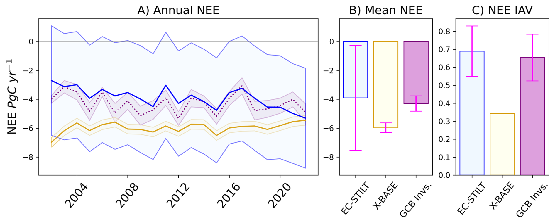
Figure 3 (A) Annual NEE integrated globally in Pg C yr⁻¹. The blue line is the mean of the EC-STILT ensemble with the shaded area representing the 1σ range across ensemble members. The yellow line is FLUXCOM X-BASE. The purple dotted line is the mean of the GCB23 ensemble of atmospheric inversions, and the shaded area is the standard deviation across the ensemble members. (B) Mean NEE integrated globally over all years. The error bars represent the 1σ range across ensemble members or published uncertainty. (C) IAV of NEE, calculated as the standard deviation of the global integral. The error bars represent the 1σ range of IAV across ensemble members.

4 Results

4.1 Global model performance

EC-STILT produces an estimate of annual global NEE of $-\mathrm{3.90}\pm \mathrm{3.63}\mathrm{Pg}\mathrm{C}{\mathrm{yr}}^{-\mathrm{1}}$, compared to the ensemble mean of atmospheric inversions in GCB23, adjusted for fire, $-\mathrm{4.29}\pm \mathrm{0.65}\mathrm{Pg}\mathrm{C}{\mathrm{yr}}^{-\mathrm{1}}$ (Fig. 3B). The RMSE of the EC-STILT annual mean with the inversion ensemble annual mean is 0.69 Pg C yr⁻¹, compared with 1.81 Pg C yr⁻¹ for X-BASE. The uncertainty of the global annual flux is very high (Fig. 3A), being driven by uncertainties in tropical NEE (Fig. 4C).

EC-STILT has learned a relationship between the input variables and NEE, which captures a large part of the natural interannual variability of global annual NEE. When producing an estimate of global NEE, the model takes the driver variables across the full land surface as inputs, but does not access any STILT footprint data, LBC or NBF data, or mole-fraction data, which are only used in constraint during training. When the model is run globally for years 2001–2021, the standard deviation of annual NEE (IAV) of the EC-STILT member mean, 0.69 Pg C yr⁻¹ (1σ), is substantially closer to the GCB23 inversion ensemble IAV of 0.65 Pg C yr⁻¹ than that of X-BASE (Fig. 3C). The R² of EC-STILT annual mean NEE with the GCB23 inversion ensemble is 0.42 (N=21 years), compared with an R² of 0.02 for X-BASE. EC-STILT IAV is consistent across the model members despite the large uncertainty in the magnitude of the flux. The mean R² between the 10 members and GCB23 inversion ensemble is 0.34 (1σ 0.08), and the mean IAV is 0.71 (1σ 0.14) Pg C yr⁻¹.

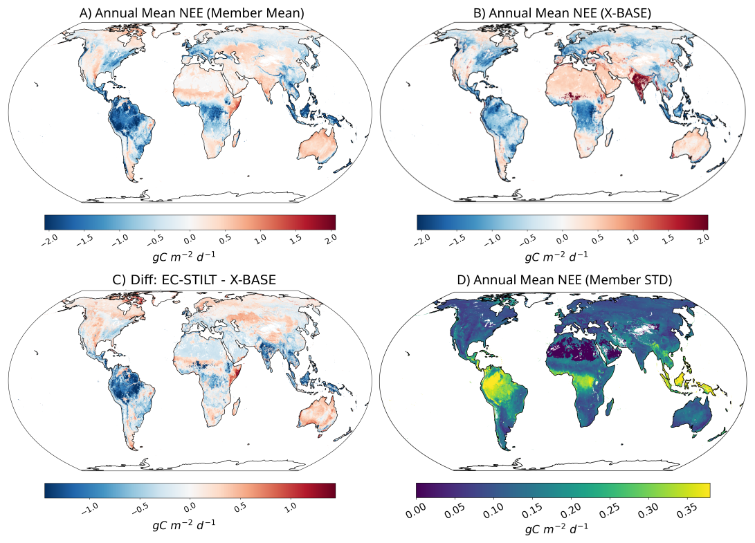
Figure 4 Spatial distribution of global annual NEE (A) Mean annual NEE for EC-STILT in $\mathrm{g}\mathrm{C}{\mathrm{m}}^{-\mathrm{2}}{\mathrm{d}}^{-\mathrm{1}}$ (B) Mean annual NEE for X-BASE in $\mathrm{g}\mathrm{C}{\mathrm{m}}^{-\mathrm{2}}{\mathrm{d}}^{-\mathrm{1}}$ (C) The difference in mean annual NEE between EC-STILT and X-BASE in $\mathrm{g}\mathrm{C}{\mathrm{m}}^{-\mathrm{2}}{\mathrm{d}}^{-\mathrm{1}}$. (D) The standard deviation of mean annual NEE for the EC-STILT 10-member ensemble in $\mathrm{g}\mathrm{C}{\mathrm{m}}^{-\mathrm{2}}{\mathrm{d}}^{-\mathrm{1}}$.

Spatially, the distribution of the mean annual NEE is largely consistent with X-BASE (Fig. 4B) with a spatial correlation of 0.71 for global mean NEE. EC-STILT has a stronger Amazonian sink and weaker boreal sink (Fig. 4C). The boreal reduction is a reduction in the length and intensity of the growing season. The EC-STILT results have removed several hotspots of source, in the Sahel and in the Indian subcontinent. These potentially unrealistic hotspots in X-BASE can be attributed to an incorrect learned relationship for crop-cover PFTs in certain dry conditions (Nelson and Walther et al., 2024). The lack of specific Plant Functional Type (PFT) information in the EC-STILT training data may be responsible for the removal of these strong sources. The large model spread in the tropics (Fig. 4D) across the Amazon Basin, the Congo Basin, and Oceania is the major source of global model spread in Fig. 3A.

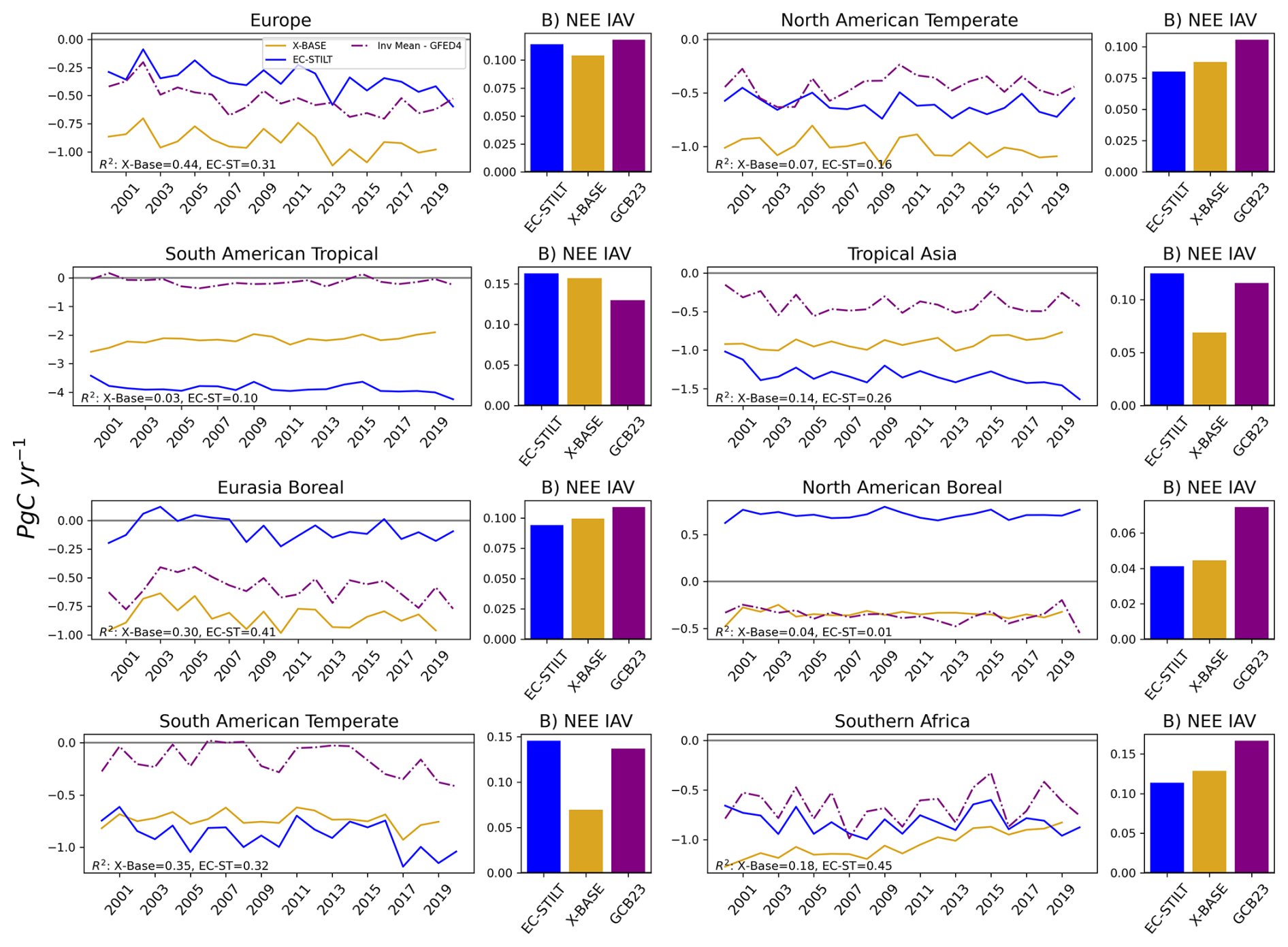
Figure 5 Annual regional NEE and IAV by TransCom region, left: the time series of the annual regional integral flux. right: the magnitude of IAV for the region. Column (A): Regional fluxes for TransCom regions directly impacted by atmospheric observations: Europe is impacted by observations in the HUN domain. Eurasia Boreal is impacted by observations in the ZOTTO domain. Both South American regions are directly impacted by observations in the ATTO domain. Column (B): Regions of similar biome and latitudinal band, by row. The blue is the ensemble mean of EC-STILT, the yellow is FLUXCOM X-BASE, the purple is the ensemble mean of the atmospheric inversions in GCB23 with GFED4.1 fire emissions removed. For each annual time series, the R² is reported for EC-STILT and X-BASE with regard to the fire-corrected ensemble mean

4.2 Regional model performance

The atmospheric constraint has a strong impact on the EC-STILT estimate of regional fluxes. Similar to the global results, EC-STILT estimates regional magnitudes of NEE which are largely inconsistent (Fig. 5, Table 2) when compared with the ensemble of atmospheric inversions used in Friedlingstein et al. (2023) corrected for fire using GFED4.1 fire emissions (Fig. 5, purple lines). The regional IAV is more in agreement with atmospheric inversions, producing similar or better R² and magnitude when compared with X-BASE regional NEE (Fig. 5, inset text, Table 2).

Regionally, there appears to be a relationship between the coverage of the eddy-covariance and atmospheric observational networks, and the impact of the atmospheric information (Table 2). For example, in Europe (Fig. 5), both the atmospheric and eddy-covariance networks are extensive. It appears that in limited cases, the atmospheric information provides some additional information on the magnitude. EC-STILT is closer to the inversion mean with an RMSE of 0.2 Pg C yr⁻¹ compared with 0.37 Pg C yr⁻¹ for X-BASE. However, the IAV is very strongly conditioned on the information in eddy-covariance data; the IAV for Europe from EC-STILT is still very similar to X-BASE with a R² of 0.86 compared with X-BASE, and 0.31 compared with the inversion mean (Table 2). The spatial pattern of summer NEE during the peak growing season (mean JJA) is very consistent between EC-STILT and X-BASE (Fig. 6) with a spatial correlation of 0.86, demonstrating the strong influence eddy-covariance information retains when used in dual-constraint. The reduced sink in the region estimated by EC-STILT (Fig. 5), appears in Fig. 6 to be largely an overall bias, rather than a learned difference in the spatial distribution of NEE.

In regions such as South American Tropical where there is limited eddy-covariance coverage to adequately constrain the model, additional atmospheric information does not improve the modeled NEE, and increases the model uncertainty. EC-STILT has moved away from the inversion mean, compared with X-BASE (RMSE of 3.73 Pg C yr⁻¹ compared with 2.05 Pg C yr⁻¹). The low R² for EC-STILT compared with both the inversion mean and X-BASE annual time series (0.10 compared with the inversions, 0.13 compared with X-BASE) indicate that neither the eddy-covariance data nor the atmospheric signal provide sufficient constraint for EC-STILT to find similar IAV to the atmospheric inversion mean, which itself might be wrong.

The increase in the IAV for the South American Temperate region demonstrates the potential for complex effects from the atmospheric constraint. The region is only directly impacted by the ATTO tower observations in unusual meteorological conditions, which is evident in the mean ATTO footprint in Fig. 2. The eddy-covariance record for the region is sparse, but may have similarities to other, more densely sampled regions. We see a small move away from the inversion mean compared with FLUXCOM X-BASE in the magnitude of NEE (RMSE of 0.74 Pg C yr⁻¹ compared with 0.59 Pg C yr⁻¹ for X-BASE), but an increase in the magnitude of IAV compared with FLUXCOM X-BASE (0.14 Pg C yr⁻¹ compared with 0.07 Pg C yr⁻¹). The atmospheric constraint has added new information about this region despite very limited direct information available in training.

Table 2 Comparison of different estimates with GCB: Column (A) shows the RMSE between the annual regional integrals in Pg C yr⁻¹ of EC-STILT and X-BASE with the atmospheric inversion ensemble mean with fire removed (Invs). Column (B) shows the R² between the annual regional integrals from EC-STILT and X-BASE with regard to the atmospheric inversion ensemble mean, and between EC-STILT and X-BASE. Bold indicates the higher relative performance between EC-STILT and X-BASE for each region and metric.

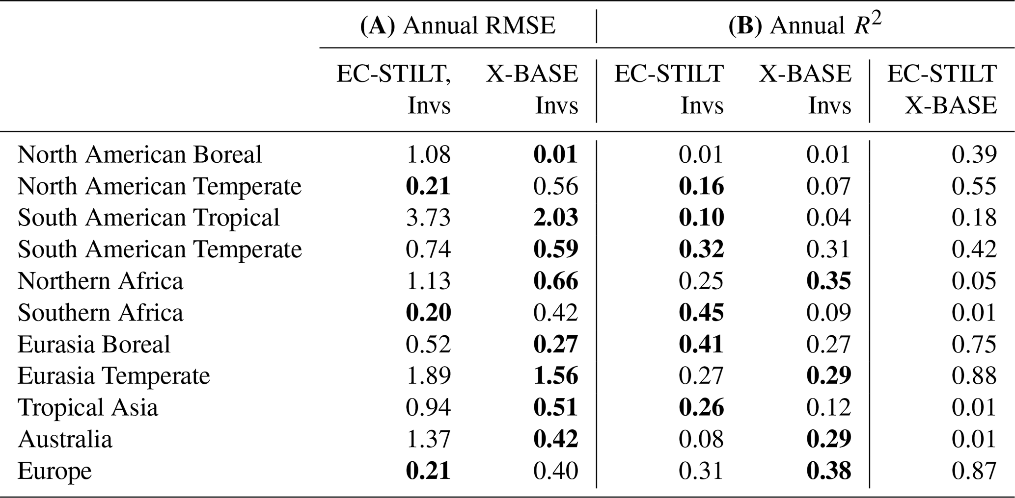
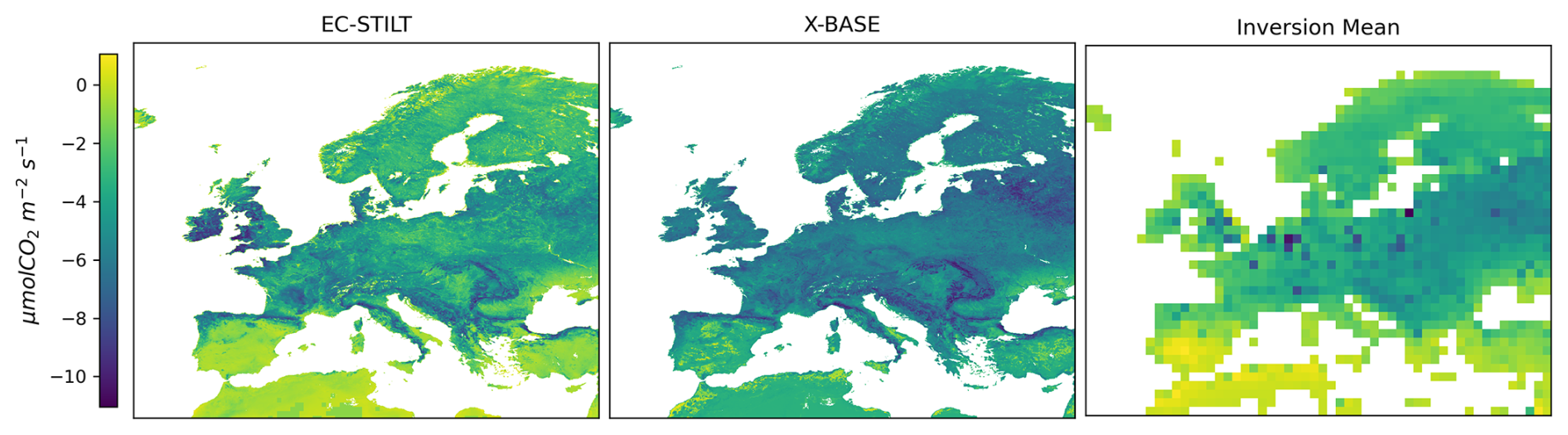
Figure 6 Mean summer NEE (JJA) in $\mathrm{\mu }\mathrm{mol}{\mathrm{CO}}_{\mathrm{2}}{\mathrm{m}}^{-\mathrm{2}}{\mathrm{s}}^{-\mathrm{1}}$ for EC-STILT, X-BASE, and the ensemble mean of the atmospheric inversions.

The atmospheric constraint also has strong effects in TransCom regions that do not directly contain or overlap the STILT regions used during training. This is because EC-STILT learns its land-surface response in environmental space of the features instead of in geographic space like an inversion. Across the globe, EC-STILT produces consistent changes over regions with similar latitude ranges (Fig. 5, right column) with a dominance of the global north in observational networks (Chu et al., 2017). The magnitude of the northern hemispheric land carbon sink is part of ongoing discrepancies in the Global Carbon Budget (O'Sullivan et al., 2024).

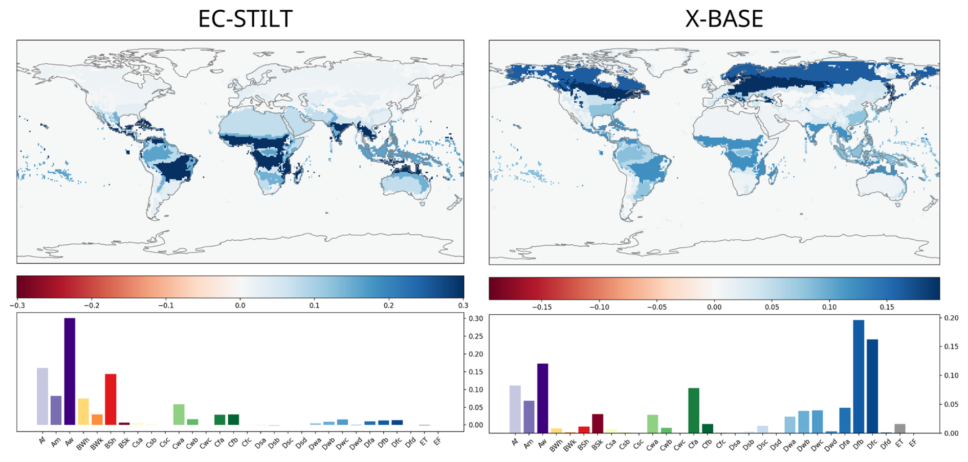
Figure 7 Attribution of IAV by Koppen-Geiger land cover class. The figure on the left is EC-STILT, the figure on right is X-BASE. The value represents the relative contribution of the region to the overall global IAV. The attribution is calculated by the covariance method described in (Lee et al., 2023) using annual detrended NEE anomalies.

4.3 IAV attribution

We find that EC-STILT attributes IAV to tropical drylands in regions Aw (tropical savanah) and Bsh (semi-arid) (Fig. 7). This contrasts with the X-BASE NEE, which attributes IAV to regions Dfb (humid continental), and Dfc (sub-arctic). Both figures show the regional contribution of IAV, relative to the overall IAV of the dataset. This metric captures only the magnitude of the contribution, not the relative accuracy of the inferred IAV, which varies strongly by region (Fig. 5). Recent studies (Metz et al., 2023, 2025; Ahlström et al., 2015; Poulter et al., 2014) also suggest that arid regions are the dominant source of the IAV in global NEE. The constraints that drive this result in our system must come from atmospheric CO₂ data, and we will try to trace the source of this information in Sect. 4.5.

4.4 Eddy-covariance site-level evaluation

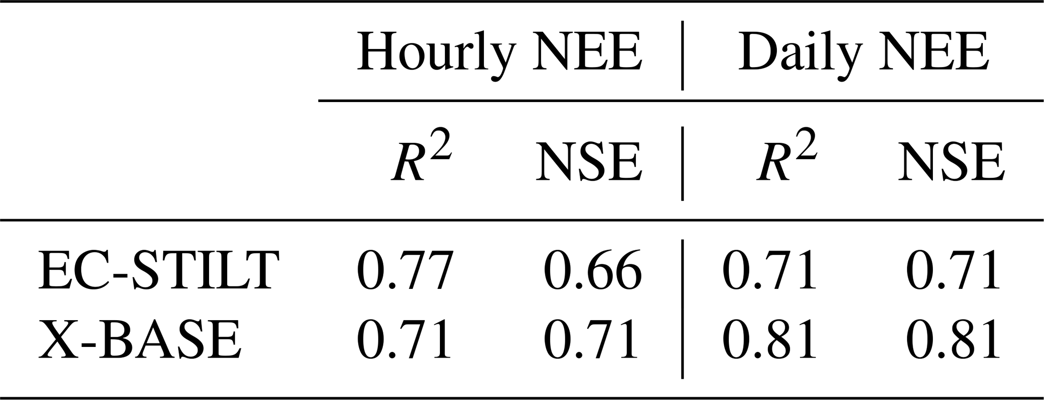
EC-STILT maintains good overall performance for NEE at the eddy-covariance site level, particularly at daily time scale. We use R² and the Nash Sutcliffe model efficiency (NSE) (Nash and Sutcliffe, 1970) to evaluate model performance with regard to the observed eddy-covariance observations, and for comparison with X-BASE. In the EC-STILT's 10-fold cross-validation for all sites (Table B4), the model achieves a median NSE of 0.66, and median R² of 0.77 for hourly fluxes (X-BASE: NSE 0.71, R² 0.71), and a median NSE of 0.76 and median R² of 0.87 for diurnal mean NEE (X-BASE: NSE 0.81, R² 0.81), when comparing the observed and simulated time series. The data used for these performance metrics are the test data, held out from each cross-validation fold, and these tests are performed using the model member which did not see these data in training.

As with regional results, the site-level performance of EC-STILT appears to be strongly influenced by the level of local constraint from eddy-covariance. Figure 8 shows the hourly and daily averaged time series of NEE for three EC sites directly impacted by the atmospheric domains, one in boreal Russia (RU-Ha1), one in a German mixed forest (DE-Hai), and one Brazilian site in the Amazon basin (BR-Sa1). In the Russian site, EC-STILT (blue line) slightly improves the estimate of the mean daily cycle of the EC observations (red line) compared with X-BASE (RMSE of 0.54 compared with 0.79). When averaged to the daily scale, both EC-STILT and X-BASE produce a similar RMSE compared with the observations. EC-STILT appears to better represent the daily signal than X-BASE with a higher R² (0.43 compared with 0.18). EC-STILT produces a range in NEE which is slightly larger than the EC record and much greater than FLUXCOM X-BASE (yellow line). Boreal regions are only moderately constrained in EC-STILT by eddy-covariance given the large difference in annual NEE between EC-STILT and X-BASE (Fig. 5). This may allow for larger differences at the site level, as the boreal observations do not sufficiently weigh against the atmospheric information.

In the German site, DE-Hai, where the constraint from eddy-covariance is strongest, EC-STILT underestimates the hourly magnitude (Fig. 8, center left) with a mean RMSE of 0.92 for EC-STILT, 0.22 for X-BASE), but still largely captures the daily NEE, but with a larger bias than X-BASE (Fig. 8, center right) with an R² of 0.61 and RMSE of 2.00 compared with an R² of 0.83 and RMSE of 1.04 for X-BASE. In the northern extra-tropics, as seen above, the marginal impact of the atmospheric information is minimized, and EC-STILT performs most similarly with X-BASE. This mismatch in the site level results is consistent with the slightly weaker regional sink seen in the northern temperate regions.

In the Brazilian site, over the mean daily cycle EC-STILT strongly underestimates the range of NEE (RMSE of 2.52), but infers a daily value when averaged, that is comparable with X-BASE (R² of 0.47 for EC-STILT and X-BASE). This may indicate that the eddy-covariance and atmospheric constraints are providing confounding information about the hourly flux, which is discussed below.

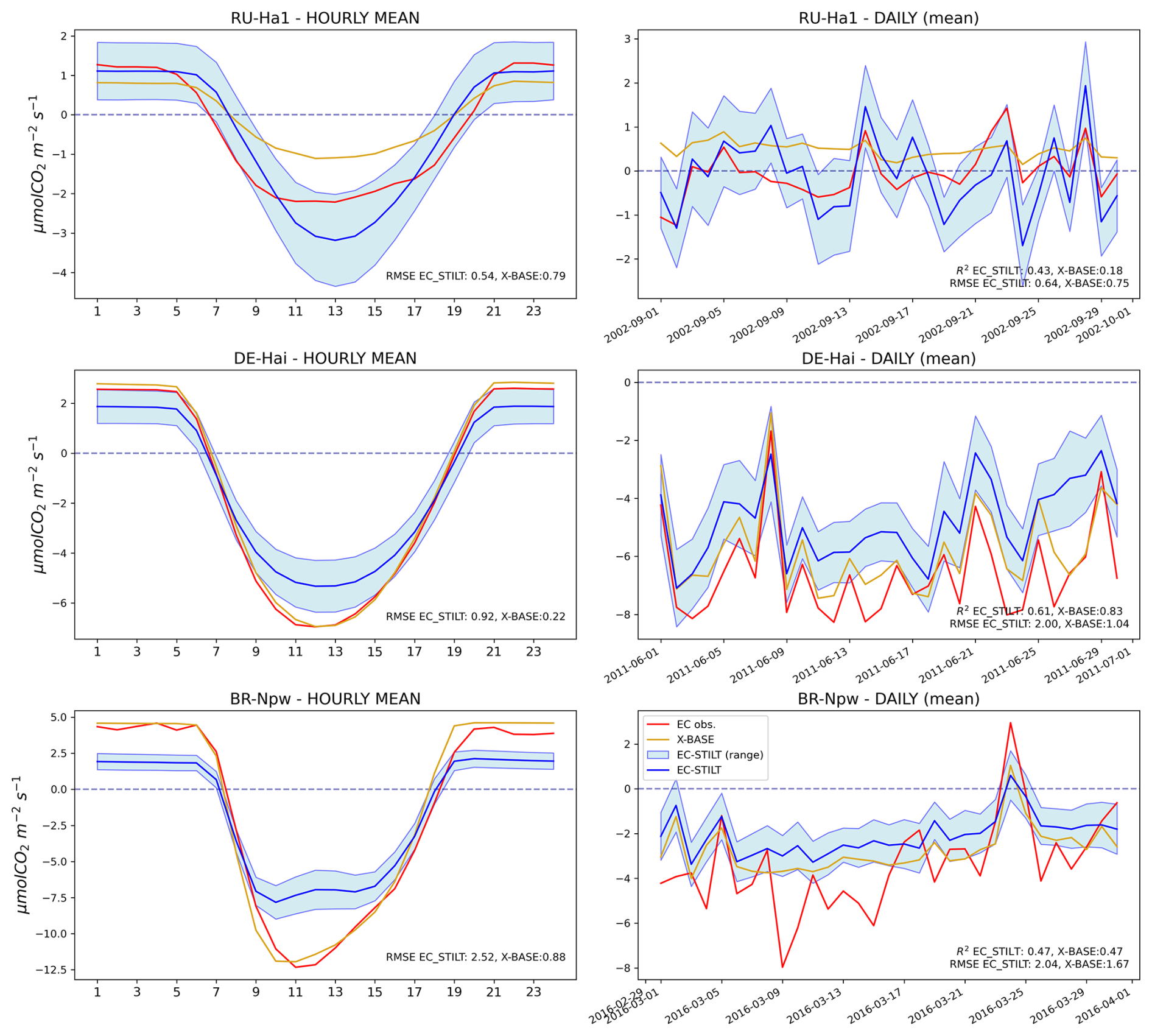
Figure 8 EC tower results across latitude bands: Each row is a tower. The left column is the mean hourly NEE, the right column is the daily mean across an example month. The blue line is the member mean of EC-STILT, the yellow line is the X-BASE NEE, and the red dotted line is the eddy-covariance observations for the tower. All values are in $\mathrm{\mu }\mathrm{mol}\mathrm{C}{\mathrm{m}}^{-\mathrm{2}}{\mathrm{s}}^{-\mathrm{1}}$.

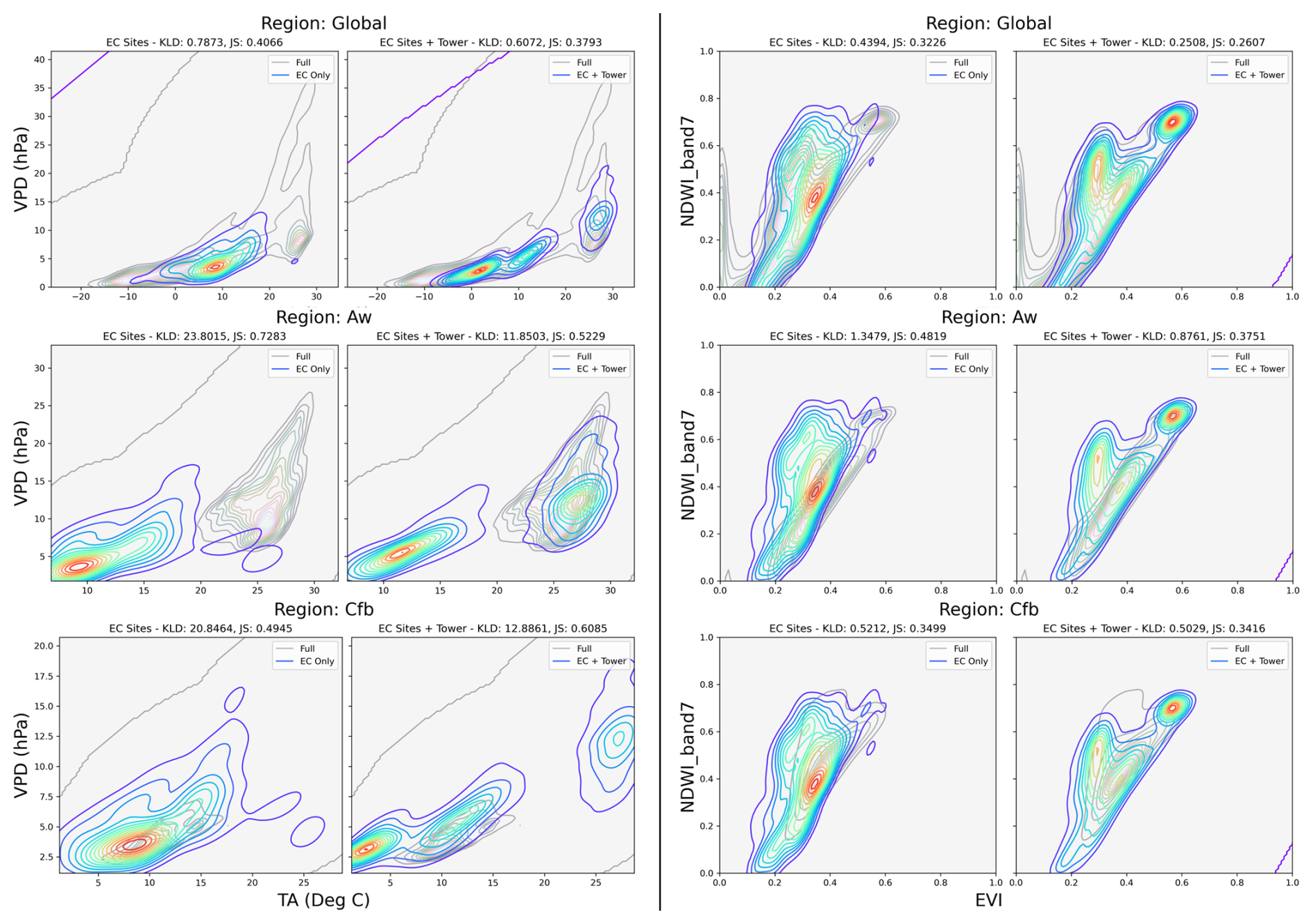
Figure 9 Comparison between training set distributions in two multivariate spaces. Both columns show the difference in distribution between the EC-only training set (left), and the EC+Towers training set (right), and how they compare with the full distribution of the global or regional data in feature space. The left is TA and VPD, the right is EVI and NDWI. The top row is the full global set, the middle row is Köppen-Geiger class Aw (Tropical Dry Winter), the bottom row is Köppen-Geiger class Cfb (Temperate Oceanic). The contour lines represent the probability distribution function (PDF) of each distribution. Two metrics are calculated for each: Kullback-Leibler (KLD) and Jennsen-Shannon divergence (JS), which are measures of distance between the two PDFs.

4.5 Learning in feature space

We analyse in Fig. 9 the coverage of the EC-only and EC-STILT training data in terms of climate and ecological space by approximating the PDF of the two joint distributions in feature-space (TA/VPD, and EVI/NDWI). We compare the relative difference in the Kullback-Leibler distance (KLD) and Jennsen-Shannon metric (JS) between the PDF of the full, or natural distribution of a random subset of all pixels, either globally or by KG class, and the two training sets (Fig. 9, Tables B1–B3). The two variable pairs were chosen to create easily interpretable visualizations. We use subsets of the full 10-dimensional distribution to save on computational costs.

At the global scale, the distribution of the EC training set is more concentrated in cooler, and moderately productive regions than the EC-STILT set (Fig. 9, top panel, compare the higher density in the warmer, more productive regions). In the second row, we can see specifically how the training data changes the representation of a region which is not directly observed. As with the global distributions, the EC-STILT distribution covers the warmer, more water-stressed regions (Fig. 9, middle panel TA/VPD) and in the wetter, more highly vegetated regions (Fig. 9, middle panel EVI/NDWI).

This distributional approach also explains why the model under-performs in regions that are directly constrained by the atmospheric towers. In the third row, the Köppen-Geiger class Cfb (Temperate Oceanic) which covers most of western Europe, we can see that in both variable sets, the EC-only distribution is closer to the natural distribution (Fig. 9, bottom row). Because of the environmental learning of EC-STILT, this means that the inclusion of atmospheric towers may reduce the model's skill in this region.

The specific impact of individual towers, and their interactions in feature space, are inconsistent across regions, variable pairs, and metrics. In Tables B1 to B3, we expand the analysis by quantifying the effect of adding or removing individual atmospheric towers from training. The optimal distribution, shown in bold, characterized by the minimum distance between the two PDFs, is enriched by adding 1–3 towers in 49 of 52 regions across both distributions (Tables B1, B2). However when the full distribution from all towers are considered (Table B3), the improvement of the tower-enriched distributions is more modest, with only 9 of 26 regions (including global) having improved coverage by the towers in both variable pairs.

5 Discussion

The core logic of our model is a synergistic sharing of information between the bottom-up and top-down constraints. The key innovation in our system is the combination of the atmospheric term with the ecosystem-level objective term derived from eddy-covariance data, and their joint projection onto a space that is not the “traditional” geographic distribution of NEE. Instead, EC-STILT learns in “environmental response” space, or a set of relations between the driver datasets (features) and the output NEE. The STILT Atmospheric transport model provides the spatiotemporal locations where ecosystem NEE variations contribute to a downwind CO₂ observation. This large number of locations over the near-field can be modeled and their output constrained by the atmospheric observation. Considered independently this is underconstrained; one atmospheric observation is insufficient to constrain the multiple modeled NEE estimates under the STILT footprint. This lack of constraint is also experienced in many inverse modeling problems using atmospheric data (see Peylin et al., 2013; Gaubert et al., 2023 for an overview). However, because the “environmental response” space of the model is conditioned by the ecosystem-level objective term, the response across the STILT footprint is tightly bound to the local, better-constrained eddy-covariance record. Learning is thus jointly informed by both data sources while maintaining, outside of the tropics, the local daily performance of bottom-up models like FLUXCOM V1 (Jung et al., 2020) and X-BASE (Nelson and Walther et al., 2024).

EC-STILT efficiently learns driver/NEE relationships globally which adds new information on the regional and global dynamics of NEE. This is demonstrated by the improved representation of IAV of global NEE (Fig. 3) and regional NEE (Fig. 5). There is no explicit representation in the training data of the atmospheric IAV; the atmospheric constraint is only present for three regional domains (around the ZOTTO, ATTO, and HUN towers). These domains were chosen to represent a tropical (ATTO), extra-tropical (HUN), and boreal (ZOTTO) eco-region. Each tower has observations across a single year (2019 for ZOTTO and Hegyhátsál, 2015 for ATTO) chosen for reasons of data availability. These relatively small samples of the available atmospheric information are sufficient to partially embed the atmospheric signal in the ecosystem response of EC-STILT, and modify the spatial and temporal distributions of estimated NEE.

We selected a limited subset of towers and training years to balance computational cost and model performance in this proof-of-concept system. The computational cost of additional towers and years is primarily associated with creating STILT footprints for a new temporal and spatial domain, which is costly both in terms of computational and human effort. We selected three sites with the specific goal to achieve good coverage of different geographic, climate and ecological zones. This precluded the use of other towers which we believe might have provided valuable constraints in training. The NOAA ObsPack data (Masarie et al., 2014) could provide a large volume of additional training data, both towers and years. Following the analysis of Sect. 4.5 we find that given the structure of our model, one might be able to increase the performance of the model with a targeted selection of towers. These would optimally represent the natural distribution of the land surface, rather than including all measurement towers across observational networks. Future experiments, similar to the EC representation analysis in Pallandt et al. (2022), can be performed to identify additional towers or years that might yield largest improvements in our predictions.

There is no explicit representation in the data of the atmospheric growth rate, nor mass-balance, yet these are reproduced to an impressive degree. The atmospheric observations are regional and instant, with no direct information on the long-term state of the atmosphere. Because the atmospheric transport system is in fact not run during the calculation of global NEE, there is therefore no atmospheric information available to EC-STILT during the creation of our global NEE data. The potentially realistic global integral and spatial distribution (Fig. 3) demonstrates that the model is able to learn a consistent ecosystem-level response globally from this sparse set of local observations with an improved representation of global dynamics. Of particular note is that these limited observations improve the estimate of IAV across the entire period of analysis, and thus learned relations hold under a range of environmental conditions in each pixel.

Although subject to large uncertainty, the magnitude of the annual flux has moved closer to the GCB23 atmospheric inversion estimate of global NEE. The global magnitude is strongly conditioned, however on the inclusion and handling of the non-biospheric flux data during training; as the total amount of NBF in a region increases, by necessity, the inferred NEE must decrease to keep the local instantaneous equation balanced (Eq. 1). The total contributions to the well-mixed atmosphere over time are complex (Ciais et al., 2022), and often not available in spatially explicit data products. The current study used fire and fossil fuel emissions, but other terms such as riverine fluxes (see Botía et al., 2025, for a discussion at the ATTO tower) may play strong local or global roles in the regional CO₂ balance, and should be included in the tower loss calculation.

Because EC-STILT has no direct access to long-term information about the state of the atmosphere, and yet produces an estimate of global annual NEE which is closer to the atmospheric inversions, there must be some information within the available training data which includes this information. The identically constructed model, trained without the inclusion of the STILT operator (Sect. 3.6) does not produce an increased IAV (see Fig. B1), which removes the influence of the model architecture. We further evaluate the influence on IAV of the LBC (Eq. 1), which is derived from atmospheric inversions. In the results from our mean-LBC model, this change did not reduce the observed IAV (see Fig. B2), which means the LBC is not responsible for the improvements in the IAV in the standard EC-STILT.

To understand the increased IAV in the tropical dry regions (see Sect. 4.3), we hypothesize that our model can better represent the local NEE responses to climate variations in these regions through a more complete representation of the natural distribution of the biophysical drivers of NEE, as shown in Fig. 9. This improvement over the information provided by the EC towers in feature-space explains EC-STILT's improved long-term performance using only a single year of observations. EC-STILT learns to represent NEE using only 10 variables at an hourly time-step. With no static variables, such as latitude, elevation, or PFT information, the model can be considered largely independent of a particular spatial domain. The model only learns to map from a training distribution of drivers to a training distribution of NEE. The quality and completeness of this training distribution determines the models capacity to capture the global phenomena.

The results from Upton et al. (2024) also support the distribution hypothesis presented above. In that study the atmospheric constraint uses a limited number of fixed pixel locations to infer regional totals. This created an NEE product which was much closer in magnitude and seasonality to an ensemble of atmospheric inversions, but did not improve the IAV. This version of atmospheric constraint does not fundamentally change the model's available view of the land surface. From this we can see that the inclusion of training data which fully includes the IAV signal, but that does not improve the distributional representation of regions from which the IAV emerges from the local variance, does not improve the model's ability to capture the IAV.

In Fig. 3A, it appears that the atmospheric signal increases the uncertainty around the magnitude and distribution of tropical NEE, when compared with X-BASE. The ensemble members show a large spread across tropical regions, and at the ecosystem-level, the ensemble mean has difficulty reproducing the magnitude of hourly observations from the eddy-covariance record (Fig. 8). EC-STILT's tropical shortcomings may be a combination of several structural factors; model type, potential mismatches in the atmospheric operator, and limited observational support, which are discussed below.

When compared with X-BASE, the core model structure is important; X-BASE is a XGBoost regressor, which have been demonstrated to be robust in this domain compared with neural networks which have more capacity to overfit (Nelson and Walther et al., 2024; Kraft et al., 2025; Jung et al., 2020). Because our objective function is sensitive to ecosystem and regional results across all three towers, it is possible that within the overall learning process, some local or regional overfitting is occurring. We attempt to reduce overfitting using early stopping of training according to the validation accuracy, and in the model using batch normalization. Potentially, this overfitting could lead to large intra-model uncertainty between neural network members compared with an XGBoost ensemble. Current implementations of XGBoost in the Python programming language (compatible with the FLUXCOM-X framework) were not considered, because they do not allow for complex objective functions with multiple terms, sensitive to different spatial scales. Any additional experimentation with different model structures was outside of the scope of this study.

The tropical response from EC-STILT is also confounded by a specific effect in the performance of the STILT atmospheric operator during training. For HUN and ZOTTO, EC-STILT achieved high Pearson's R values (0.65–0.8) for the inferred and observed land contribution to the CO₂. However for ATTO, although the RMSE during training between the inferred and observed land contribution was similar to the training RMSE for HUN and ZOTTO, Pearson's R was near zero (0.0–0.15, see Fig. A5). This means that the system was able to infer the correct magnitude of the contribution, but unable to get the signal correctly located in time. This poor temporal registration may be attributed to a missing NBF contribution to the signal which has a strong temporal component, such as the mentioned riverine evasion of CO₂ (Botía et al., 2025). Or the issue may be with the transport model or its meteorological forcing. Our STILT footprints are calculated at 0.25° spatial resolution. This resolution was chosen because of computational constraints in our training. It is possible that this spatial resolution does not adequately capture some aspect of the atmospheric processes in the tropics. In relation to the relatively small contribution of intra-model uncertainty within LPDMs (Hegarty et al., 2013), meteorological uncertainty is a more important term in the overall transport uncertainty (Angevine et al., 2014). However, it was out of scope for the current work to estimate that uncertainty with regard to the output STILT sensitivities and and resulting concentration estimates. Lastly, the temporal issue at ATTO may have to do with the rate of air exchange through the canopy. This could introduce a time lag into the release of CO₂ out of the canopy and into the free atmosphere (Faassen et al., 2024).

Both bottom-up (Chu et al., 2017) and top-down (Palmer et al., 2019) observational records are limited and uncertain in the tropics. This limited record forces a data-driven model to extrapolate its response for a range of missing or under-sampled parts of the tropical distribution of the driver variables. It is unrealistic for a model constrained only by the existing observational record to move meaningfully beyond previous work on estimating tropical fluxes. Although the boreal region around ZOTTO is also subject to the same uncertainties with regard to the observational record, the uncertainty relative to the magnitude of the flux does not impact global results to the same extent.

In the eddy-covariance site results (Fig. 8) we may see an example of atmospheric information confounding and augmenting the eddy-covariance signal. Both boreal and tropical regions are less well constrained by eddy-covariance than the northern extra-tropics, which increases the marginal impact of the atmospheric constraint. EC-STILT was able to reproduce both the Russian site's (RU-Ha1) eddy-covariance hourly time series and the ZOTTO time series with high fidelity. Indeed, EC-STILT estimates an hourly variability which is higher than the hourly eddy-covariance data. In the Brazilian site (BR-Npw), where EC-STILT was unable to reproduce the ATTO time series, we see the eddy-covariance finding a low-variability estimate of the daily mean. This may represent confounding between constraints.

While the absolute increase in the R² of IAV with regard to the GCB23 inversions is modest (0.42 for EC-STILT, 0.02 for X-BASE), it represents a meaningful increase over previous data-driven flux models (Jung et al., 2019; Nelson and Walther et al., 2024). As seen above in Sect. 4.2 and Fig. 7, EC-STILT improves the estimation of IAV in regions in the Southern Hemisphere which are known to contribute to a large fraction of the global IAV. However EC-STILT fails to improve the representation of IAV in the Northern Hemisphere, or where the EC observational record dominates. Therefore, the modest gain in R², can be seen as a meaningful gain in the representation of the land surface in regions which are otherwise poorly represented in the EC record.

5.1 Future work

This study finds improvement in a number of important metrics in a bottom-up NEE model that is additionally constrained by three atmospheric tall-towers over one year. As noted above, neither the eddy-covariance record nor the atmospheric observational record have strongly representative global coverage, and additional atmospheric information over new geographic regions could be a benefit. Therefore an important future development of a dual-constrained model is the inclusion of additional tower and non-tower data streams: Additional tall towers could provide stronger constraint in well-measured regions. Non-tower data could be leveraged to provide information on regions that are poorly covered by the current observational network. The current model could run, as-is, against aircraft observations. With a modification of the STILT transport system in the objective function, the structure of this study would allow a bottom-up model to be constrained by satellite retrievals of total column CO₂ (XCO₂). XCO₂ observations could be selected according to their potential to include biomes of specific interest in their upwind footprints. This would enrich our capacity to model NEE across un- and under-sampled biomes. This extension into XCO₂ introduces several possible issues: to model the full column of CO₂, multiple STILT footprints must be run for every observation at different elevations (Wu et al., 2018), and modeled fluxes transported multiple times. This may be a technical challenge to build effective training systems. The inclusion of the full column CO₂ may dilute the available information on the biogenic flux in the observation, reducing the information gain to the bottom-up model.

The performance of EC-STILT in the tropics show the limitations of adding atmospheric information without adequate support in the eddy-covariance record. In the harmonized model described above, the ecosystem-level information appears to provide the “backbone” of the model's performance. Future modeling efforts will benefit from the ongoing efforts to improve and enlarge the corpus of available eddy-covariance sites and data, such as a potential extension of the FLUXNET 2015 dataset (Pastorello et al., 2020). As the eddy-covariance record better describes and constrains key biomes, additional atmospheric constraint may be able to provide improved information on the larger dynamics of regional and global NEE, while reducing the uncertainty.

An important aspect of transport modeling which is not addressed in the current study is the impact of model and meteorological uncertainty. In our analysis, we treat the output of the STILT model as definitive, relative to the meteorological fields in ECMWF short-term forecast. Computational schemes for addressing model uncertainty, multi-LPDM ensembling, or in-model ensembling for STILT by sampling within the stochastic particles could be attempted, without a major increase in computational and I/O workload. In this study, STILT runs are forced with ECMWF short-term forecast data (Botia et al., 2022), and the model is trained using ERA5 reanalysis data. Using identical meteorological data for STILT and the model drivers may also reduce uncertainty.

Conceptually, the current work accounts for two major terms in the non-biogenic flux budget; fires and fossil fuel emissions. In the Amazon and in boreal Russia, fire is the largest and the most relevant term, as the term accounts for both fire, and also for part of the instantaneous flux from land-cover/land-use change associated with biomass burning (Cochrane and Laurance, 2008). In the European domain, fossil fuels are the dominant non-biogenic flux signal. As noted in the Sect. 2, NEE at the eddy-covariance tower and atmospheric CO₂ are not directly comparable. The dual-constraint in this study is created using the residual of an observation and non-biogenic fluxes. Any biogenic or non-biogenic flux terms which are not included, or adequately represented temporally and spatially will bias the atmospheric target that the model is trying to match in training. An example of this would be the non-fire disturbance fluxes, or regrowth after disturbance. Another potentially important term is the instantaneous riverine flux of CO₂, coming from lateral riverine transport. These terms could push the relative carbon balance towards CO₂ release (disturbances) or towards CO₂ assimilation (regrowth), and during retraining the model would attempt to match this new local target balance. As seen above, because of the distributional nature of the model's learning and inference, this new local balance could modify the global NEE response. This reduces the effectiveness of the technique. Any additional spatially explicit NBF data may therefore, improve this comparison, and increase the fidelity of the overall magnitude and may reduce the uncertainty in the global result.

6 Conclusions

This study demonstrates a novel method for combining bottom-up and top-down information in the objective function of a data-driven flux model. We wanted to test the effectiveness of a physics-based operator that transports modeled flux density into atmospheric concentration. And we wanted to determine whether a temporally and geographically-sparse constraint could produce valid global results. The EC-STILT model in this study is still strongly conditioned by the bottom-up constraint from eddy-covariance, and so maintains the strengths of the overall bottom-up approach, but now with access to information on land surface far beyond the eddy-covariance network.

A classical top-down atmospheric inversion matches the observed atmospheric signal but lacks the framework to accurately distribute that signal down into geographic/biophysical space. Bottom-up models can translate EC measurements into their latent space, but do not have any additional information about how inferred fluxes influence the global signal. In contrast, our hybrid system in this study can take information from the atmospheric observations and accurately distribute it into the learned latent space of the model. Because this latent space still contains information from the eddy-covariance record, this allows for a valid mapping down from the atmosphere to the model, and from the model to an estimate of NEE at multiple scales which is comparable both with both atmospheric and ecosystem-level observations. Using our system, a dual-constrained model sits directly between bottom-up and top-down approaches, directly addressing their limitations while maintaining their advantages.

Appendix A: Data

(Garcia et al., 2016)(Kutzbach, 2021)(Posse et al., 2016)(Wohlfahrt et al., 2016)(Cleverly and Eamus, 2016b)(Beringer and Hutley, 2016c)(Meyer et al., 2016)(Pendall and Griebel, 2016)(Beringer and Hutley, 2016b)(Beringer and Hutley, 2016f)(Beringer and Hutley, 2016e)(Schroder et al., 2016)(Beringer and Hutley, 2016a)(Macfarlane et al., 2016)(Beringer and Hutley, 2016d)(Liddell, 2016)(Cleverly and Eamus, 2016a)(Woodgate et al., 2016)(Beringer et al., 2016b)(Beringer et al., 2016a)(Arndt et al., 2016)(Beringer and Walker, 2016)(Team and Centre, 2022b)(Team and Centre, 2022b)(RI, 2021a)(Team and Centre, 2022b)(Team and Centre, 2022b)(Team and Centre, 2022b)(Vourlitis et al., 2022)(Saleska, 2016)(Goulden, 2016d)(Staebler, 2022)(Knox, 2022)(Christen and Knox, 2022)(Wagner-Riddle, 2021)(McCaughey, 2016)(Black, 2021)(Amiro, 2016b)(Goulden, 2016a)(Goulden, 2016b)(Goulden, 2016c)(Goulden, 2016g)(Goulden, 2016e)(Goulden, 2016f)(Black, 2016b)(Black, 2016a)(Margolis, 2016)(Amiro, 2016c)(Amiro, 2016a)(Amiro, 2016d)(Arain, 2016b)(Arain, 2016a)(Arain, 2022b)(Arain, 2016c)(Arain, 2022a)(Nouvellon, 2016)(Team and Centre, 2022b)(Team and Centre, 2022b)(Team and Centre, 2022b)(Team and Centre, 2022b)(Team and Centre, 2022b)(Ammann, 2016)(Team and Centre, 2022b)(Zhang and Han, 2016)(Dong, 2016)(Shi et al., 2016)(Zhou and Yan, 2016)(Chen, 2016k)(Shao, 2016b)(Tang et al., 2016)(Wang and Fu, 2016)(Shao, 2016a)(Team and Centre, 2022b)(Sigut et al., 2016)(Team and Centre, 2022b)(Team and Centre, 2022b)(Team and Centre, 2022b)(Team and Centre, 2022b)(Team and Centre, 2022b)(Team and Centre, 2022b)(Team and Centre, 2022b)(Team and Centre, 2022b)(Team and Centre, 2022b)(Team and Centre, 2022b)(Team and Centre, 2020a)(Team and Centre, 2022b)(Team and Centre, 2022b)(Lindauer et al., 2016)(Knohl et al., 2016)(Team and Centre, 2022b)(RI, 2022b)(Team and Centre, 2022b)(Team and Centre, 2022b)(Schneider and Schmidt, 2016)(Klatt et al., 2016)(Bernhofer et al., 2016)(Team and Centre, 2022b)(Sachs et al., 2016)(Pilegaard and Ibrom, 2016)(Olesen, 2016)(RI, 2022b)(Team and Centre, 2022b)(Team and Centre, 2022b)(Team and Centre, 2022b)(Poveda et al., 2016)(Team and Centre, 2022b)(Team and Centre, 2022b)(Team and Centre, 2022b)(Team and Centre, 2022b)(Reverter et al., 2016b)(Reverter et al., 2016a)(Team and Centre, 2022b)(Lohila et al., 2016)(Team and Centre, 2022b)(Team and Centre, 2022b)(Aurela et al., 2016a)(Team and Centre, 2022b)(Team and Centre, 2022b)(Aurela et al., 2016b)(RI, 2022b)(Team and Centre, 2022b)(Team and Centre, 2022b)(RI, 2022b)(Team and Centre, 2022b)(Team and Centre, 2022b)(Team and Centre, 2022b)(Team and Centre, 2022b)(Berbigier and Loustau, 2016)(RI, 2022b)(Team and Centre, 2022b)(Ourcival, 2016)(RI, 2022b)(Team and Centre, 2022b)(Valentini et al., 2016b)(RI, 2022b)(Hansen, 2016)(Lund et al., 2016b)(Lund et al., 2016a)(Team and Centre, 2022b)(Team and Centre, 2022b)(Team and Centre, 2022b)(RI, 2022b)(Sabbatini et al., 2016c)(Sabbatini et al., 2016a)(Sabbatini et al., 2016b)(Matteucci, 2016)(Team and Centre, 2022b)(Valentini et al., 2016a)(Gruening et al., 2016b)(Cescatti et al., 2016)(Team and Centre, 2022b)(RI, 2022b)(Team and Centre, 2022b)(Spano et al., 2016)(Manca and Goded, 2016)(Team and Centre, 2022b)(Valentini et al., 2016c)(Papale et al., 2016)(Team and Centre, 2022b)(Gruening et al., 2016a)(Team and Centre, 2022b)(Kotani, 2016b)(Kotani, 2016a)(Yepez and Garatuza, 2021)(Kosugi and Takanashi, 2016)(Dolman et al., 2016a)(Team and Centre, 2020a)(Wolf et al., 2016b)(Wolf et al., 2016a)(Griffis and Roman, 2021)(Merbold et al., 2016)(Dolman et al., 2016b)(Team and Centre, 2022b)(Team and Centre, 2022b)(Belelli et al., 2016)(Ardö et al., 2016)(Team and Centre, 2022b)(Team and Centre, 2022b)(Team and Centre, 2020a)(Team and Centre, 2022b)(Team and Centre, 2022b)(Team and Centre, 2022b)(Christensen, 2016)(Boike et al., 2016)(Tagesson et al., 2016)(Billesbach et al., 2022)(Billesbach et al., 2016b)(Billesbach et al., 2016a)(Biraud et al., 2022)(Torn, 2016b)(Torn, 2016a)(Zona and Oechel, 2016a)(Euskirchen, 2022b)(Euskirchen, 2022c)(Euskirchen, 2022d)(Euskirchen, 2022a)(Rey-Sanchez et al., 2022b)(Rey-Sanchez et al., 2022a)(Goldstein, 2016)(Huggins, 2021)(Huggins, 2022c)(Huggins, 2022a)(Huggins, 2022b)(Chen and Chu, 2016b)(Desai, 2022a)(Desai, 2022c)(Desai, 2022d)(Desai, 2022b)(Bowling, 2016)(Oikawa, 2021)(Massman, 2016)(Massman, 2022)(Meyers, 2016b)(Forsythe et al., 2021)(Goslee, 2022)(Munger, 2016)(Liu et al., 2022)(Hollinger, 2022)(Matamala, 2016)(Euskirchen et al., 2022a)(Euskirchen et al., 2022b)(Zona and Oechel, 2016b)(Vivoni and Perez-Ruiz, 2022)(Brunsell, 2022a)(Brunsell, 2022b)(Drake and Hinkle, 2016a)(Drake and Hinkle, 2016b)(Hinkle, 2022)(Meyers, 2016a)(Fares, 2016)(Desai, 2016c)(Novick and Phillips, 2022)(Wood and Gu, 2022)(Law, 2016c)(Law, 2022)(Law, 2016a)(Law, 2016e)(Law, 2016d)(Law, 2016b)(Litvak, 2021)(Sturtevant et al., 2016)(Torn and Dengel, 2021)(Blanken et al., 2022)(Suyker, 2022)(Suyker, 2016b)(Suyker, 2016a)(Silveira, 2021)(Bohrer, 2021)(Bohrer and Kerns, 2022)(Chen et al., 2016)(Desai, 2016d)(Kobayashi and Suzuki, 2016)(Flerchinger, 2022c)(Baker et al., 2022)(Baker and Griffis, 2022a)(Baker and Griffis, 2021)(Baker and Griffis, 2022b)(Flerchinger and Reba, 2022)(Flerchinger, 2022a)(Flerchinger, 2022b)(Kurc, 2022)(Scott, 2016a)(Scott, 2016b)(Shortt et al., 2022)(Kusak et al., 2022)(Ewers and Pendall, 2016)(Desai, 2016b)(Baldocchi and Ma, 2016)(Valach et al., 2021)(Sturtevant et al., 2022)(Chamberlain et al., 2022)(Sanchez et al., 2016)(Valach et al., 2022)(Baldocchi, 2016)(Bohrer, 2022)(Gough et al., 2016)(Gough et al., 2022)(Baldocchi et al., 2016)(Desai, 2016a)(Chen and Chu, 2016a)(Scott, 2016d)(Chen, 2016g)(Chen, 2016e)(Chen, 2016j)(Chen, 2016b)(Chen, 2016d)(Chen, 2016a)(Chen, 2016h)(Chen, 2016i)(Chen, 2016c)(Chen, 2016f)(Litvak, 2022)(Scott, 2016c)(Network), 2022)

Table A1 Citation data for the 294 sites used in training.

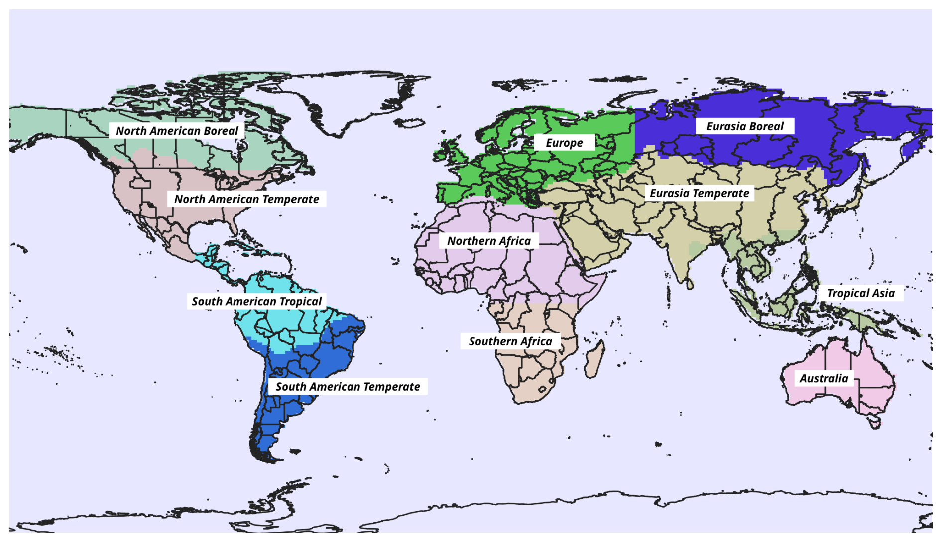
Figure A1 TransCom land regions.

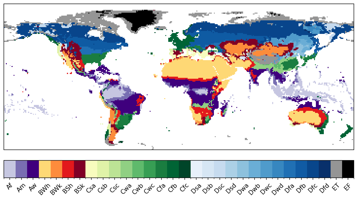
Figure A2 Köppen-Geiger (KG) classification system from Beck et al. (2018).

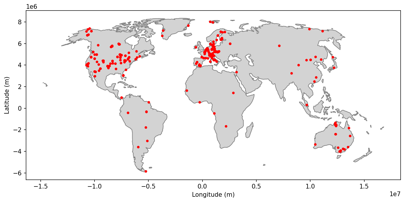
Figure A3 Eddy-covariance towers used in training.

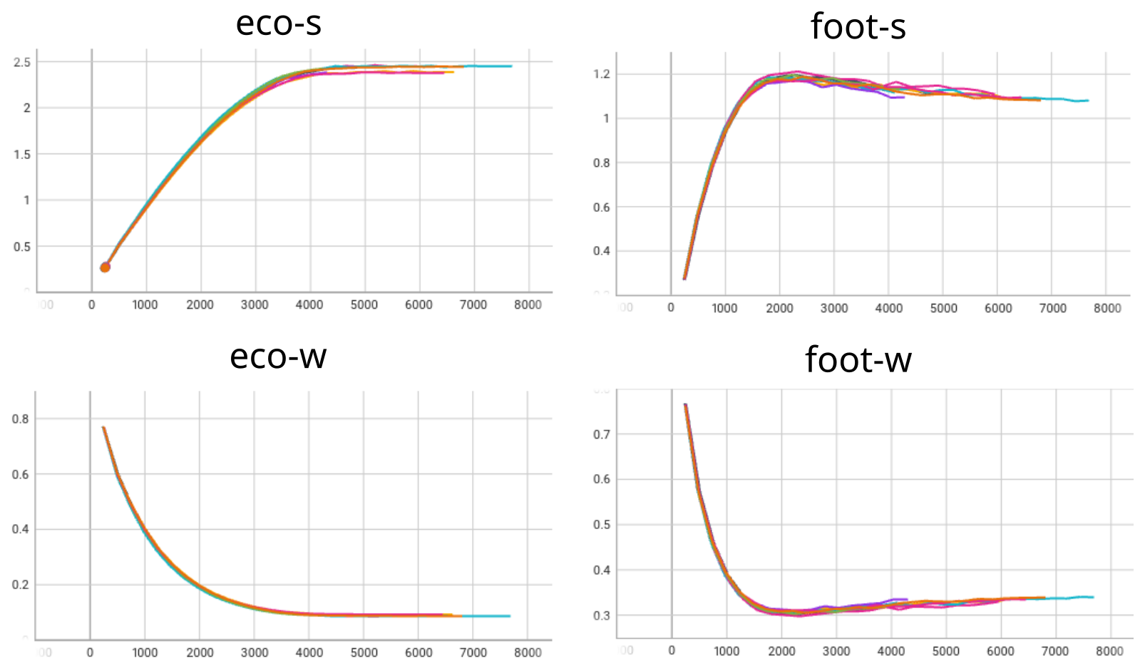
Figure A4 Evolution of weighting-scheme variables during model training. The colored lines represent the 10 members from the k-folds cross validation.

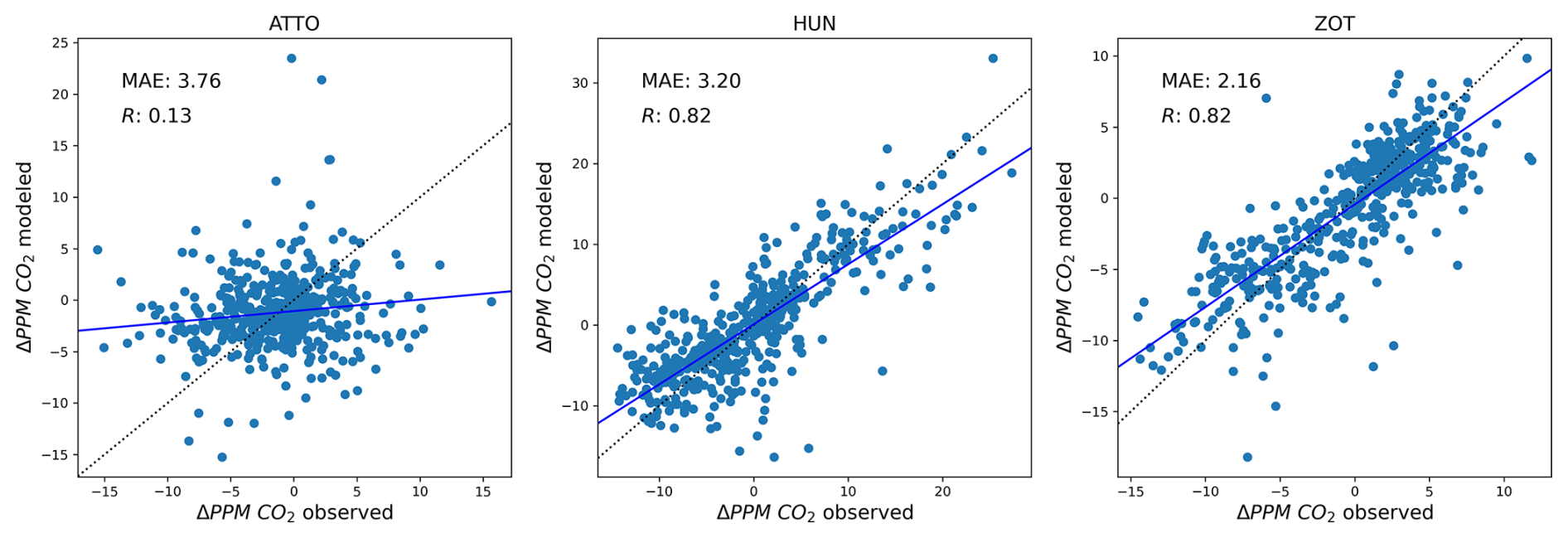
Figure A5 Per-tower representative STILT operator training performance (estimated ΔPPM CO₂ and observed ΔPPM CO₂) for the final epoch of one ensemble member. The black, dotted line is the one-to-one line. The blue line is the regression line. The mean absolute error (MSE) and Pearson's R are reported for each tower.

Appendix B: Results

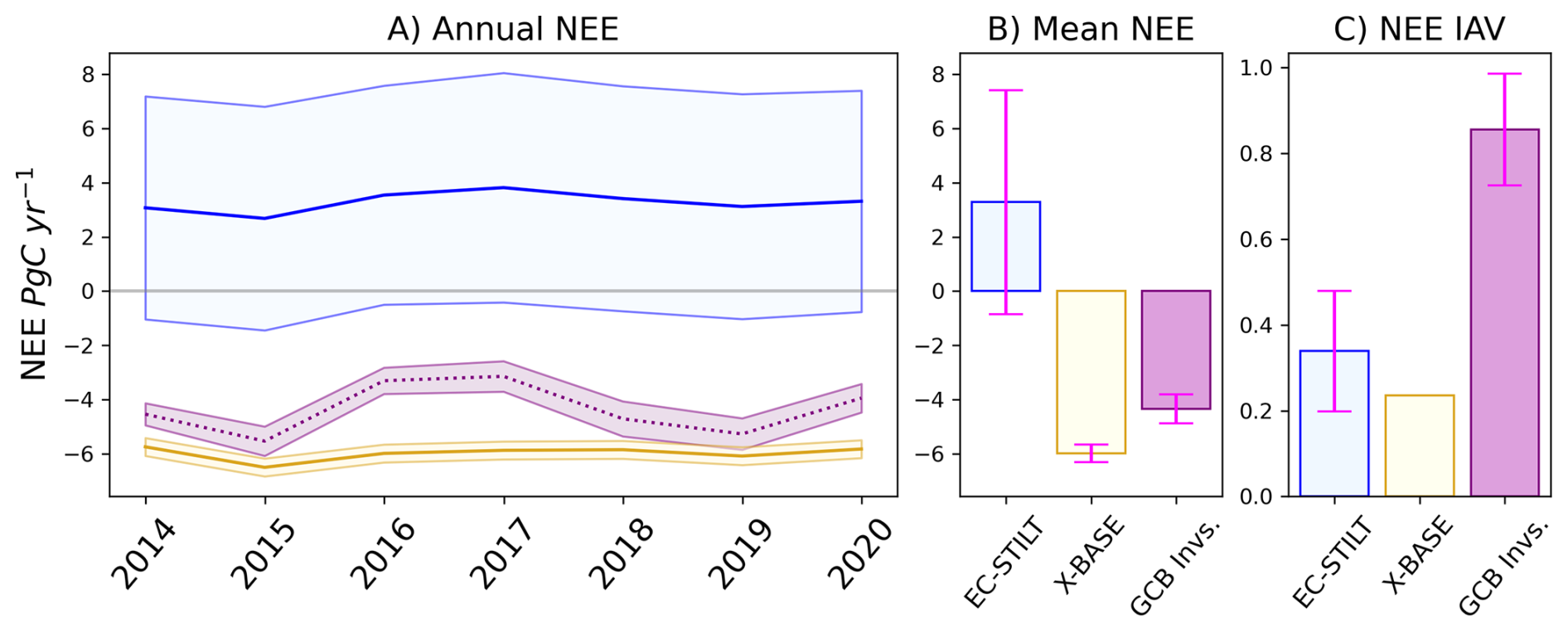
Figure B1 Model ensemble trained without STILT operator: (A) Annual NEE integrated globally in Pg C yr⁻¹. The blue line is the mean of the EC-NO-STILT ensemble with the shaded area representing the 1σ range across ensemble members. The yellow line is FLUXCOM X-BASE. The purple dotted line is the mean of the GCB23 ensemble of atmospheric inversions, and the shaded area is the standard deviation across the ensemble members. (B) Mean NEE integrated globally over all years. The error bars represent the 1σ range across ensemble members or published uncertainty. (C) IAV of NEE, calculated as the standard deviation of the global integral. The error bars represent the 1σ range of IAV across ensemble members.

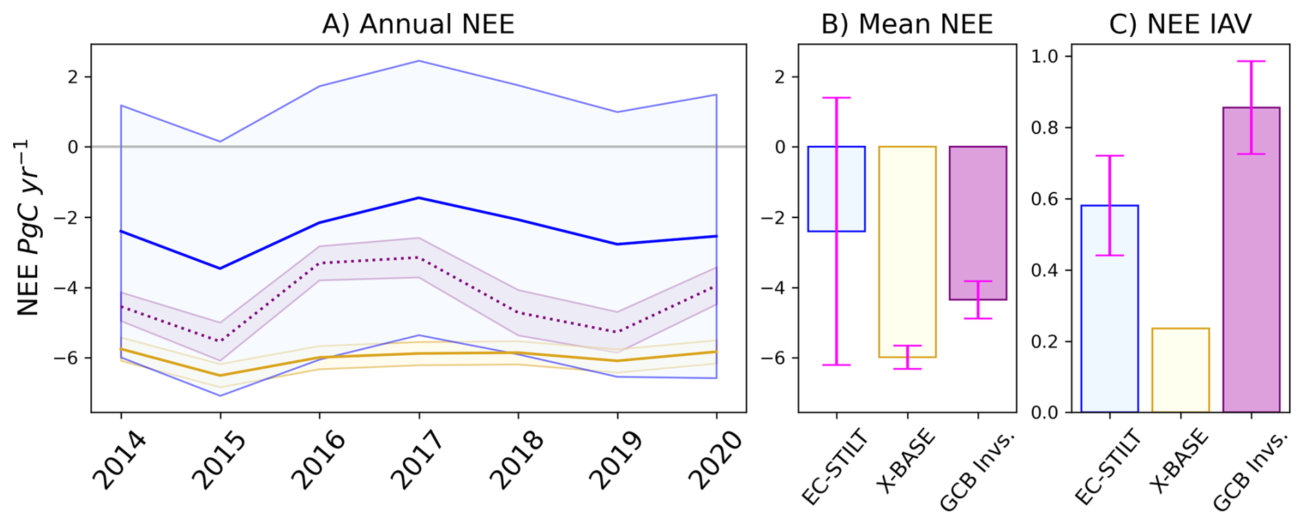
Figure B2 Model ensemble trained a mean LBC term: (A) Annual NEE integrated globally in Pg C yr⁻¹. The blue line is the mean of the meanLBC ensemble (n=3) with the shaded area representing the 1σ range across ensemble members. The yellow line is FLUXCOM X-BASE. The purple dotted line is the mean of the GCB23 ensemble of atmospheric inversions, and the shaded area is the standard deviation across the ensemble members. (B) Mean NEE integrated globally over all years. The error bars represent the 1σ range across ensemble members or published uncertainty. (C) IAV of NEE, calculated as the standard deviation of the global integral. The error bars represent the 1σ range of IAV across ensemble members.

Table B1 TA/VPD: Kullback-Leibler distance (KLD) and Jennsson-Shannon metric (JS) between the estimated global and regional PDFs of training data subsets and the estimated PDF of the natural distribution. Columns represent the eddy-covariance (EC) training data, EC plus all three tall towers (EC + Tower), and EC training data plus single towers (e.g. ATTO represents EC plus ATTO), and plus two towers, notated by the tower removed from consideration (e.g. NO-ATTO represents EC + HUN + ZOT). The bold entry represents the lowest distance by metric. Multiple bold entries indicate identical performance across different training sets.

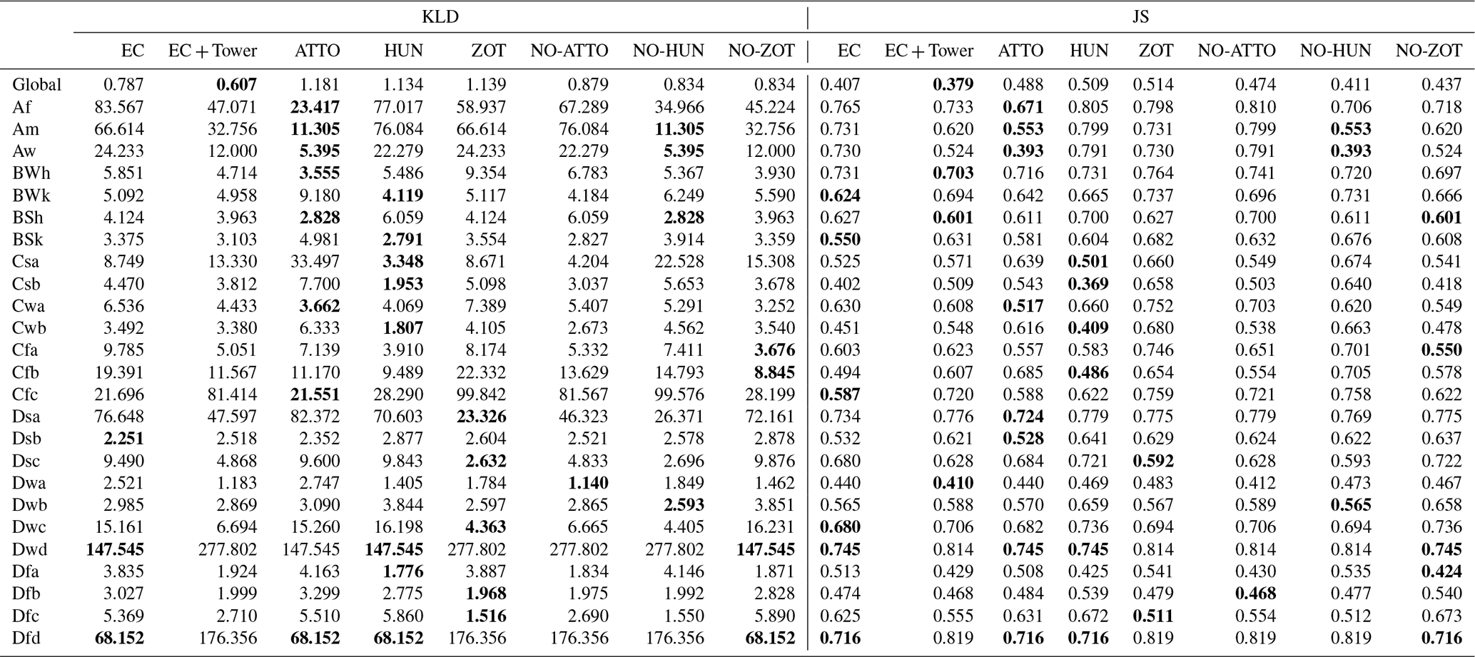
Table B2 EVI/NDWI: Kullback-Leibler distance (KLD) and Jennsson-Shannon metric (JS) between the estimated global and regional PDFs of training data subsets and the estimated PDF of the natural distribution. Columns represent the eddy-covariance (EC) training data, EC plus all three tall towers (EC + Tower), and EC training data plus single towers (e.g. ATTO represents EC plus ATTO), and plus two towers, notated by the tower removed from consideration (e.g. NO-ATTO represents EC + HUN + ZOT). The bold entry represents the lowest distance by metric.

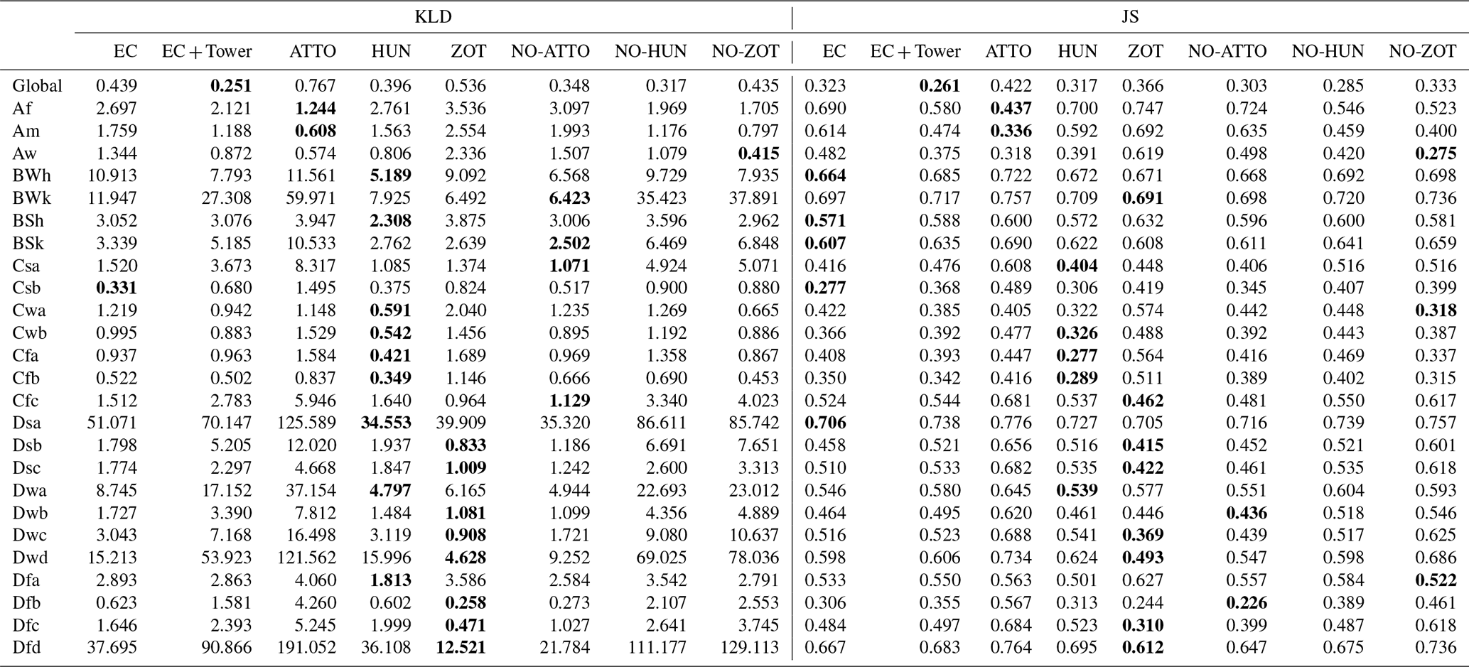
Table B3 EC-only/Tower-enriched: Kullback-Leibler distance (KLD) and Jennsson-Shannon metric (JS) between the estimated global and regional PDFs of training data subsets and the estimated PDF of the natural distribution. For each set of variables and metric, columns represent the eddy-covariance (EC) training data, and the EC plus all three tall towers (EC + Tower). The bold entry represents the lowest distance by metric and variable set.

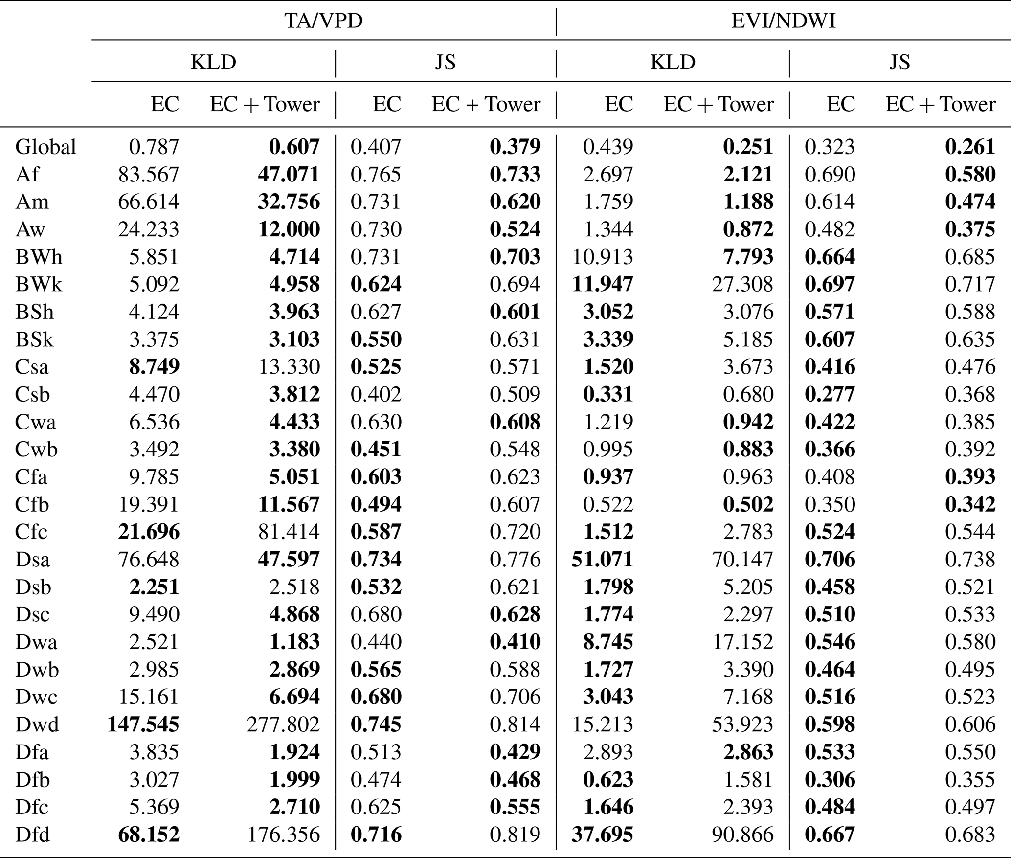
Table B4 Cross-validation results for EC-STILT and X-BASE. The columns are hourly and daily R² and NSE for the sites that were reserved for validation during testing.