
the Creative Commons Attribution 4.0 License.
the Creative Commons Attribution 4.0 License.
 | 16 Nov 2026
Constraining the hydrogen soil sink and photochemical source: insights from atmospheric H2 inversions (2003–2023)

Joram J. D. Hooghiem
Maarten C. Krol
Wouter Peters
Hydrogen (H2) is expected to become an increasingly important energy carrier during the energy transition, likely leading to higher atmospheric H2 levels due to losses during production, transport, storage and usage of hydrogen. Multiple studies have shown this could impact atmospheric composition through interactions with the hydroxyl radical. However, the magnitude of this impact remains uncertain due to large uncertainties in the global H2 budget, particularly in the soil sink and photochemical source. To address this, we present a spatiotemporally resolved H2 budget derived using atmospheric inversions with the TM5 chemical transport model. With this approach, we infer a global mean soil sink of 52.8 [47.8–56.7] Tg yr−1 and a photochemical source of 34.6 [29.2–38.2] Tg yr−1 over 2003–2023. Relative to Ouyang et al. (2025), we estimate a soil sink that is 45 % and 35 % weaker in the Middle East and Oceania, and 45 % and 70 % stronger in South America and Russia, respectively. Our results further suggest that variability in the observed H2 growth rate between 2003–2023 was primarily driven by changes in the photochemical source from CH4 oxidation, together with a declining global soil sink at a mean rate of 0.23 Tg yr−2. Finally, we infer a sensitivity of the soil sink to the El Niño–Southern Oscillation, strongest over diffusion-limited soils in tropical South America, with increased uptake during drier El Niño conditions and reduced uptake during wetter La Niña conditions.
- Article
(14558 KB) - Full-text XML
- BibTeX
- EndNote


Global hydrogen (H2) demand has roughly doubled over the last two decades and is projected to keep increasing during the ongoing energy transition (IEA, 2019, 2023). As a result, atmospheric H2 levels may increase due to unavoidable losses across production, transport, storage, and usage of hydrogen (Ocko and Hamburg, 2022; De Kleijne et al., 2024). This could impact tropospheric methane (CH4) and ozone (O3), as well as stratospheric water vapour levels, through interactions with the hydroxyl radical (OH). Together, these effects yield a 100-year global warming potential (GWP100) for hydrogen of 11.6 ± 2.8 (Sand et al., 2023), meaning that 1 kg of H2 emitted has a climate impact equivalent to 11.6 ± 2.8 kg of CO2 emitted over a 100-year horizon. The uncertainty in the GWP100 estimate arises primarily from a limited understanding of the global hydrogen budget. Particularly, the photochemical H2 source and the soil sink, representing the two largest fluxes in the budget, are highly uncertain (see Table 2). According to the recent comprehensive assessment of the global H2 budget by Ouyang et al. (2025), the remaining terms in the budget, including biomass burning, fossil fuel combustion, ocean emissions, land emissions from N2 fixing bacteria, and the OH sink, are comparatively well constrained in magnitude. This study provides the most detailed uncertainty assessment of the global hydrogen budget to date, based on a diverse ensemble of bottom-up approaches, and will therefore be referred to frequently throughout the remainder of this paper.
The global photochemical H2 source from formaldehyde (CH2O) photolysis is the most uncertain source in the H2 budget. It arises from multiple pathways reflecting the diversity of CH2O precursors and is typically quantified using global chemical transport model simulations. The contribution from CH4 oxidation, the dominant precursor pathway via CH2O, is relatively well constrained. This is because CH4 is a long-lived greenhouse gas with well-characterised global atmospheric abundances, constrained by extensive surface and satellite observations. In contrast, the contribution from oxidation of anthropogenic and biogenic Volatile Organic Compounds (VOCs) is more uncertain, reflecting shorter atmospheric lifetimes and less well-constrained emission inventories of these precursors.
The global H2 soil sink is the largest and most uncertain term in the H2 budget (Sand et al., 2026), as shown in Table 2. Its uncertainty arises from a complex dependence on multiple interacting environmental drivers, including soil moisture, soil temperature, and soil organic carbon content. It also exhibits strong spatial variability, with field measurements showing that fluxes can differ substantially between sites only a few kilometres apart (Cowan et al., 2025). Estimates of the global H2 soil sink rely on parametrisations predominantly derived from field measurements at mid-latitude Northern Hemisphere sites (Ehhalt and Rohrer, 2009). This introduces a representativeness bias, as tropical regions, which are expected to show high soil H2 uptake (Tardito Chaudhri and Stevenson, 2025), are not represented in the underlying observations. In addition, parametrisations are limited by the lack of accurate, high-resolution forcing data for key drivers such as soil moisture and soil temperature, further introducing uncertainty in global flux estimates. Finally, a key limitation of most bottom-up studies is that their fluxes are not propagated through three-dimensional transport models, making it impossible to verify their consistency with long-term global H2 observations.
To overcome some of these challenges, a top-down approach can be used. Here, bottom-up fluxes serve as a first guess and are subsequently adjusted using H2 mole fraction measurements. These atmospheric observations integrate information from sources and sinks over large spatial scales, thereby reducing the influence of local variability and allowing fluxes to be constrained without detailed knowledge of all underlying environmental drivers. Previous top-down studies with two-dimensional box models by Rhee et al. (2006) and Xiao et al. (2007) suggested that the soil sink and photochemical source were substantially larger than found in bottom-up studies (see Table 2). Subsequent studies employing three-dimensional chemical transport models yielded budgets more consistent with bottom-up literature, but relied on shorter observational records. For example, Pison et al. (2009) used observations from a single year (2004), Yver et al. (2011) relied on relatively few stations, mostly in Europe, and Bousquet et al. (2011) analysed observations from 1991–2004. Since then, the observational record has expanded considerably, providing a clear opportunity to revisit this problem. Furthermore, none of these studies included observations from South America or tropical Africa, regions expected to exhibit some of the largest photochemical source and soil sink fluxes globally.
In this study, we present an updated, comprehensive regional-to-global H2 budget for 2003–2023, derived from atmospheric H2 inversions using the TM5 chemical transport model. We build on the work of Pieterse et al. (2013), incorporating several updates and improvements, including updated emission inventories, a more sophisticated soil sink scheme, improved OH fields, and higher horizontal and vertical resolution. We also exploit observations from an expanded network of H2 monitoring sites, providing stronger constraints on regional fluxes. Finally, we evaluate our simulated H2 mole fractions against independent observations from four aircraft campaigns.
The following sections describe the observations (Sect. 2.1), modelling framework (Sect. 2.2), and implementation of hydrogen sources and sinks (Sect. 2.3) used in this study. We then describe the setup of the forward simulations used to pre-balance global mean sources and sinks (Sect. 2.4), followed by the setup of the detailed inversion experiments (Sect. 2.5).
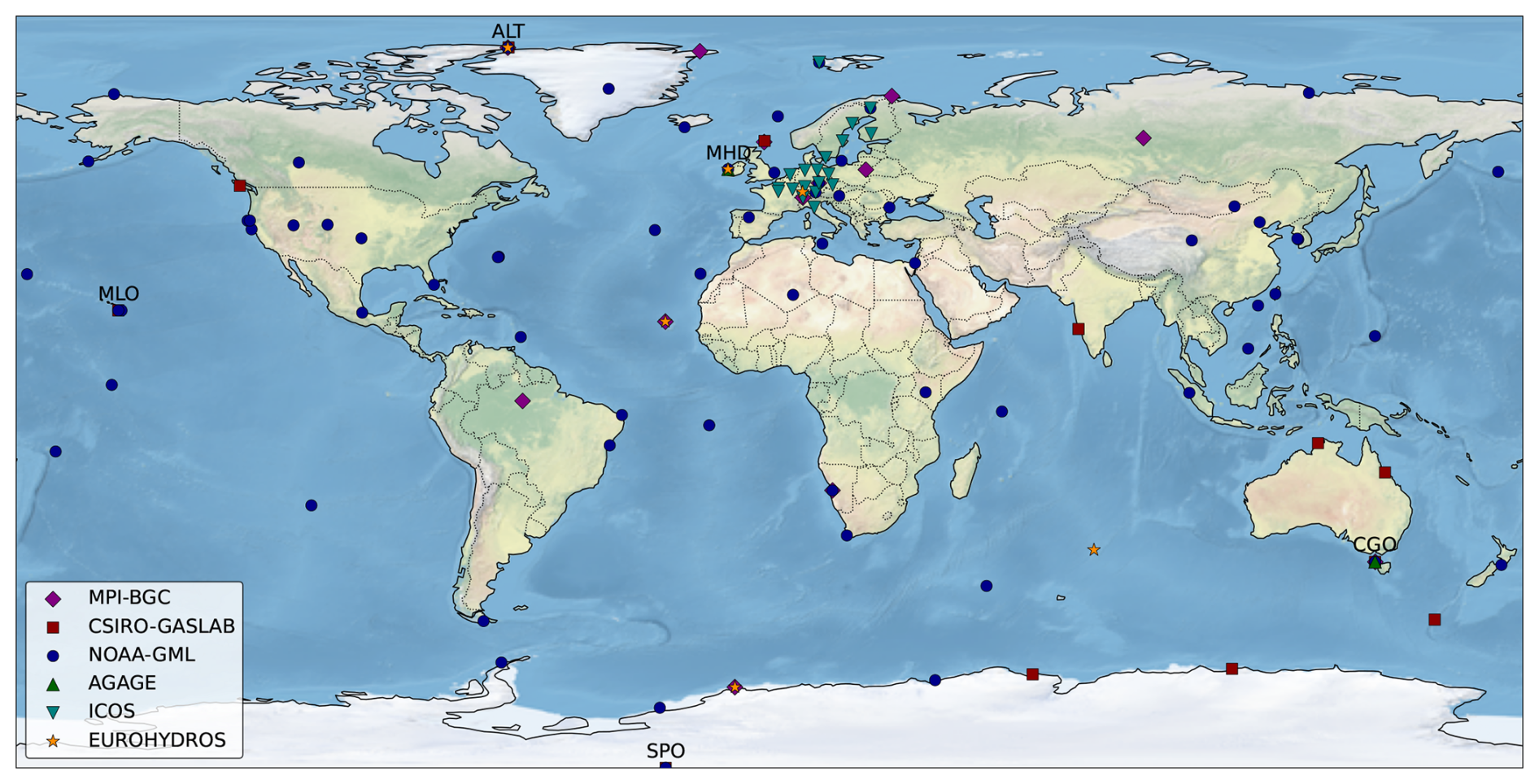
Figure 1Global distribution of H2 monitoring sites (N=96) from the NOAA-GML, CSIRO-GASLAB, MPI-BGC, AGAGE, ICOS, and EUROHYDROS networks. Only sites with measurements at any time during 2003–2023 are included, with individual sites covering different sub-periods. Key sites are labelled for later reference.
2.1 Observations
We use H2 mole fraction observations from multiple surface flask networks, including EUROHYDROS (EUROpean network for atmospheric HYDRogen Observations and Studies; Batenburg et al., 2011), NOAA-GML (National Oceanic and Atmospheric Administration Global Monitoring Laboratory; Pétron et al., 2024), CSIRO-GASLAB (Commonwealth Scientific and Industrial Research Organisation Global Atmospheric Sampling Laboratory; Krummel et al., 2025), MPI-BGC (Max Planck Institute for Biogeochemistry; Jordan et al., 2024), and ICOS (Integrated Carbon Observation System; Apadula et al., 2025). We also use in situ measurements from AGAGE (Advanced Global Atmospheric Gases Experiment; Prinn et al., 2025). All data are reported on the MPI-2009 calibration scale (Jordan and Steinberg, 2011). Observations span 96 monitoring sites, with some locations sampled by multiple networks (Fig. 1). Most sites do not provide continuous coverage over the full analysis period (2003–2023); details on measurement periods and sampling frequency for each network are provided in Table F1 of the Appendix. All data are filtered to retain observations representative of background conditions using available quality control and representativity flags. For NOAA-GML, only measurements analysed with a helium pulse discharge detector are used. For independent evaluation of our optimised H2 mole fractions, we use aircraft measurements from NOAA-GML (Sweeney et al., 2015; McKain et al., 2022). These measurements include continental aircraft profiles over the United States, as well as the HIPPO (HIAPER Pole to Pole Observations; Wofsy, 2011; Wofsy et al., 2017) and ATom (Atmospheric Tomography Mission; Montzka et al., 2019; Thompson et al., 2022; Wofsy et al., 2021) campaigns, which provide pole-to-pole sampling of background atmospheric conditions across multiple altitudes. Additionally, we also use aircraft measurements from IAGOS-CARIBIC (In service Aircraft for a Global Observing System – Civil Aircraft for the Regular Investigation of the Atmosphere Based on an Instrument Container; Batenburg et al., 2016) for independent evaluation.
2.2 Modelling framework
We use the TM5 three-dimensional chemical transport model (Krol et al., 2005), driven by meteorological fields from ERA5 (ECMWF ReAnalysis v5; Hersbach et al., 2020), to simulate atmospheric H2 mole fractions. To estimate the magnitude and spatial distribution of monthly global H2 fluxes, TM5 is coupled with the CarbonTracker data assimilation system (Van Der Laan-Luijkx et al., 2017), which employs an ensemble Kalman filter.
2.3 Implementation of hydrogen sources and sinks
Our modelling framework builds on Pieterse et al. (2013), with several updates and improvements. We include H2 surface emissions as monthly fluxes at 1°×1° resolution. Fossil fuel emissions are calculated by scaling sector-specific CO emissions from CAMS v6.2 (Copernicus Atmosphere Monitoring Service; Soulie et al., 2024) to H2 using corresponding emission factors from CEDS (Community Emissions Data System; Hoesly et al., 2018). This approach exploits the shared origin of H2 and CO in fossil fuel combustion and related processes such as the water–gas shift reaction, while leveraging the relatively well-constrained global CO emissions inferred from satellite observations. Oceanic H2 emissions are prescribed from an annually repeating monthly climatology based on the oceanic CO flux distribution of Conte et al. (2019), scaled to a global annual emission of 5 Tg yr−1 (Price et al., 2007). This approach is based on the shared biological origin of H2 (Walter et al., 2016) and CO (Gros et al., 2009) in the ocean, and uses CO fluxes as a proxy for biological activity. Similarly, land H2 emissions are prescribed from an annually repeating monthly climatology based on biogenic CO land fluxes from MEGAN (Model of Emissions of Gases and Aerosols from Nature; Guenther et al., 2012) for 2010, scaled to a global annual emission of 3 Tg yr−1 (Conrad et al., 1989; Conrad, 1996; Pieterse et al., 2011). Finally, biomass burning emissions are taken from GFED5 (Global Fire Emissions Database v5; Van Der Werf et al., 2025).
We pre-calculated three-dimensional photochemical source fields from CH2O photolysis to use in our system, by running a full-chemistry version of TM5-MP (Williams et al., 2017) with the CB05 chemical mechanism (Carbon Bond v5; Yarwood et al., 2005). The full-chemistry model included 51 species and 156 reactions, covering the oxidation chains of CH4 and other key VOCs. Since H2 was originally treated as a fixed species in CB05, we added H2 production from CH2O photolysis (Reaction R1) to the chemical scheme using the photolysis rate constant from Sander et al. (2006). The remaining CH2O loss pathways were already included in CB05 (Reactions R2 and R3).
We performed the full-chemistry simulations at 3°×2° horizontal resolution with 34 vertical levels over 2003–2023. Chemistry was driven by the H2 fluxes described in this section, together with CH4 fields nudged towards surface observations and CMIP6 (Coupled Model Intercomparison Project Phase 6; Feng et al., 2020) emissions for almost all remaining species. We derived separate photochemical H2 source fields for production from isoprene oxidation (hereafter the isoprene source) and from oxidation of all remaining VOCs, dominated by CH4 oxidation (hereafter the non-isoprene source). This allows for separate specification of the flux uncertainties, with higher confidence in the non-isoprene H2 source due to the well-characterised global abundance of CH4. We derived the source partitioning from five sensitivity simulations in which isoprene emissions were scaled by a factor 1.0 to 0.6 (in steps of 0.1), yielding an essentially linear response in the photochemical H2 source (R2=0.999). We then estimated the non-isoprene H2 source by extrapolating this relationship to zero isoprene emissions, with the isoprene H2 source calculated as the residual relative to the base simulation (with a factor of 1.0). We have relatively high confidence in the spatial distribution of our combined photochemical H2 source fields, based on a comparison of simulated CH2O mole fractions with CH2O aircraft observations from the ATom campaign, as discussed in Sect. A of the Appendix.
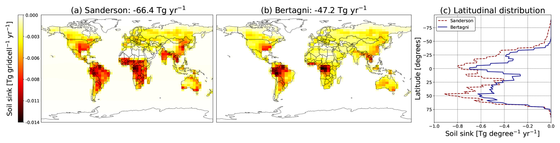
Figure 2H2 annual mean soil sink fluxes (2003–2013) from simulations with the Sanderson (a) and Bertagni (b) scheme. These simulations were performed using a photochemical source of 38.2 Tg yr−1 (scaled by a factor of 0.7 for consistency with the literature) and no additional scaling of the soil sink (factor 1.0). Panel (c) shows the corresponding latitudinal H2 flux distributions.
We calculate soil sink fluxes at 1°×1° resolution following scenario S3c of Pieterse et al. (2013). This approach uses the TM5 dry deposition scheme, which applies a series-resistance formulation including time-varying aerodynamic and soil resistances to compute the H2 deposition velocity. The soil sink flux is then calculated using the deposition velocity and the near-surface H2 mass mixing ratio in the lowest model layer at each 3 h time step of the simulation. In the standard configuration, the soil resistance component follows the Sanderson et al. (2003) scheme. This scheme defines seven ecosystem regions representing broad ecosystem categories rather than explicit soil types, and is driven by soil moisture and soil temperature fields from ERA5 (Hersbach et al., 2020). We also implemented an alternative deposition scheme in which the soil and snow resistance formulations are replaced by those of Bertagni et al. (2021). Here, the soil resistance equations include nonlinear soil moisture dynamics and depend on soil moisture, soil temperature, and porosity across eleven soil texture classes. We obtained the required soil property fields from the Global Land Data Assimilation System (GLDAS; Rodell et al., 2004). Figure 2 highlights the main differences between the two schemes. On average, the Sanderson scheme yields a 40 % larger global soil sink than the Bertagni scheme for 2003–2013. It also yields stronger uptake in subtropical regions such as northern India and South Africa, and weaker uptake in arid regions such as the Sahara and the Tibetan Plateau relative to the Bertagni scheme. Throughout the remainder of this paper, we will refer to simulations using the Sanderson and Bertagni schemes as “Sanderson” and “Bertagni”, respectively (e.g. Sanderson inversion or Bertagni inversion).
We calculate the chemical H2 sink by oxidation with OH based on Reaction (R4) using the reaction rate constant from JPL (Jet Propulsion Laboratory; Percival and Sander, 2026). We use 3 h OH fields from CAMS EAC4 (Copernicus Atmosphere Monitoring Service ECMWF Atmospheric Composition Reanalysis 4; Inness et al., 2019) for the period 2003–2023 at 1°×1° resolution with 60 vertical levels, together with the three-dimensional H2 fields from the TM5 simulation.
In the stratosphere, we prescribe H2 mole fractions based on the CH4–H2 relationship of McCarthy (2004), following Pieterse et al. (2013). This is needed since TM5 was mainly designed to simulate the troposphere and lacks advanced stratospheric chemistry and high vertical resolution. For example, important reactions such as methane oxidation by chlorine radicals and electronically excited oxygen atoms, as described by Rahn et al. (2003) and Röckmann et al. (2003), are not included in TM5. To define the troposphere–stratosphere boundary, above which the H2 mole fractions are fixed, we use the latitude-dependent pressure threshold given by Eq. (1) of Pieterse et al. (2011). To drive the parametrisation, we use monthly CH4 fields from CAMS EAC4 at 1°×1° resolution, interpolated to 34 vertical levels.
2.4 Balancing global mean sources and sinks
To explore the wide range of photochemical source and soil sink estimates in the literature (Table 2), we use the TM5 model to identify source–sink configurations consistent with the observed evolution of global H2 mole fractions. We perform forward simulations for 2003–2013 at 6°×4° resolution with 25 vertical levels, applying uniform global scaling factors to the soil sink and combined photochemical H2 source. We then compute four metrics using the NOAA ccgcrv curve fitting package (Thoning et al., 1989; NOAA Global Monitoring Laboratory, 2026) based on the simulated and observed H2 mole fractions at five NOAA-GML sites (ALT, CGO, MHD, MLO, SPO): (a) detrended RMSE, (b) difference between simulated and observed mean growth rate at MLO, (c) absolute difference between simulated and observed interhemispheric gradient between ALT and SPO, and (d) absolute difference between simulated and observed seasonal amplitude at MHD. The configurations that perform best across these metrics are then used as the starting point for the subsequent Bayesian optimisation of H2 sources and sinks.
2.5 Setup of the inversion experiments
We use the CarbonTracker Europe v3 framework (Van Der Laan-Luijkx et al., 2017) to perform a month-by-month optimisation of the soil sink and photochemical H2 source. We run the inversion over the 2003–2023 period, with atmospheric transport simulated at 3°×2° horizontal resolution and 34 vertical levels. We use an ensemble size of 300 members to balance performance and computational cost. We optimise the photochemical source by applying monthly regional scaling factors to the prior photochemical production fields described in Sect. 2.3. For the soil sink, we do not directly scale the fluxes as calculated within the respective schemes, as test inversions showed that this led to unstable Kalman filter performance. Instead, we optimise linearised representations of the soil sink fluxes, as explained in Sect. 2.5.1.
2.5.1 Linearisation of soil sink and stratospheric flux
The soil sink and stratospheric fixing terms were linearised in the inversions to ensure stable Kalman filter performance. This addresses a well-known limitation in Kalman-based flux optimisation arising from strongly non-linear flux-state dependencies or from initial states far from the solution, as documented in carbon cycle inversions (Tolk et al., 2011). Such conditions are applicable here, since test inversions showed that large posterior-prior adjustments in H2 mole fractions (up to 100 ppb) were required to reconcile global mass balance, large-scale gradients, and seasonal cycles. Since both processes depend directly on the H2 mole fraction, this introduced a non-linear coupling between fluxes and mole fractions that led to instability of the Kalman filter. Therefore, daily linearised soil sink and stratospheric fluxes were obtained from forward simulations at 3°×2° resolution with 34 vertical levels over 2003–2023, using the Sanderson and Bertagni schemes under the best-performing source-sink configurations identified in Sect. 3.1 in relation to four observational metrics. Our inversion results support the linearisation, as posterior mole fractions remain close to the prior (Sect. 3.2.1). Specifically, mean posterior deviations are −2.0 % (Bertagni inversion) and −11.6 % (Sanderson inversion), corresponding to flux differences of 1.1 and 6.6 Tg yr−1 under a fully first-order soil sink formulation. We deem this acceptable, as the differences are modest compared to the range of alternative prior soil sink perturbations (± 13 Tg yr−1 relative to the base case) explored in the sensitivity analysis, which nevertheless showed convergence towards a stable posterior soil sink magnitude (Appendix Sect. D).

2.5.2 Spatial discretisation
We optimise the soil sink over the spatial regions used within each scheme: seven ecosystem regions for Sanderson and eleven soil texture classes for Bertagni (Table 1). In each region, the optimisation adjusts the magnitude of the linearised daily soil sink fluxes on 1°×1° resolution, which are effectively treated as negative surface emissions within the inversion. To introduce additional interhemispheric degrees of freedom in the statevector, the regions are subdivided at 25° N, resulting in 14 and 22 regions, respectively (Fig. F1 in the Appendix). This choice accounts for the asymmetric land distribution between hemispheres and approximately balances land area between the northern and southern portions of the modelling domain. For the photochemical source, we separately optimise pre-calculated H2 production fields from isoprene and non-isoprene oxidation, to account for differences in the uncertainties of their three-dimensional distributions. The isoprene H2 source is optimised over the same 14 Sanderson regions as the soil sink, assuming that isoprene emissions are predominantly biogenic and ecosystem-dependent. This approach reflects the short atmospheric lifetime of isoprene, which leads to relatively localised CH2O production from its oxidation with respect to the underlying emissions. We optimise the non-isoprene H2 source using 1° latitudinal bands, with a correlation length scale of 1000 km, yielding roughly 18 degrees of freedom from pole to pole. This reflects the relatively long atmospheric lifetime of CH4, the dominant precursor of CH2O in this term, yielding a relatively uniform spatial H2 production pattern from its oxidation.
2.5.3 Temporal correlation structure
We apply a temporal correlation structure to the prior flux to ensure coherent adjustments to fluxes over seasonal and sub-seasonal timescales. Annually recurring changes to the seasonal cycle are imposed through flux correlations between the same month of year (MOY) of neighbouring years. This correlation drops off exponentially with a decay constant (σMOY) of 36, 24, and 12 months for the non-isoprene H2 source, soil sink, and the isoprene H2 source respectively. These σMOY values were derived from the sensitivity tests described in Sect. C1 of the Appendix. In addition, a month-to-month correlation is imposed across all prior fluxes to reduce the degrees of freedom and to avoid unrealistically high flux variability. This correlation (σMON) decays exponentially with a time scale of 3 months.
2.5.4 Statevector element uncertainty
To reflect the relative confidence in our prior fluxes, we assign statevector element uncertainties across space and time of 7.5 % for the soil sink, 5 % for the isoprene H2 source, and 2.5 % for the non-isoprene H2 source. We note that these values can not be directly interpreted in flux space (e.g. to compute prior uncertainties in Tg yr−1), as their effect on fluxes is mediated by the inversion and cannot be directly inferred.
2.5.5 Model-data mismatch
We define a model–data mismatch (MDM) of 3.0 ppb for most sites, following Pison et al. (2009). The MDM represents the uncertainty assigned to each observation, accounting for measurement, transport, and representativeness errors. The MDM determines the relative weight of each observation in the inversion with smaller values imposing a stronger constraint on the posterior flux. Our value of 3.0 ppb exceeds the measurement uncertainties reported in Pétron et al. (2024), allowing for errors beyond instrumental uncertainty. For Deep Southern Hemisphere sites, we assign a MDM of 1.5 ppb, reflecting lower transport errors (Appendix Sect. C2). When multiple observations are available on a given day for a site, the MDM for that day is scaled by the square root of the number of observations to avoid overweighting. We exclude the NOAA-GML surface flask sites AMY (Anmyeon-do, South Korea) and SDZ (Shangdianzi, China) from the optimisation, as they are strongly influenced by local fossil fuel emissions that cannot be resolved at the model's spatial resolution. Aircraft H2 observations are also excluded to retain them for independent evaluation.
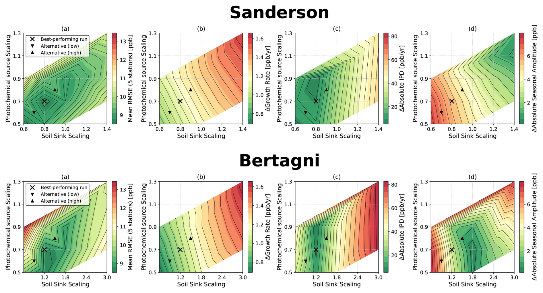
Figure 3Sensitivity analysis for various source-sink configurations using the Sanderson (top row) and Bertagni (bottom row) schemes. Shown are: (a) mean RMSE across five stations (ALT, CGO, MHD, MLO, SPO); (b) Δ Growth Rate at MLO; (c) Δ Interpolar Difference (ALT-SPO); and (d) Δ Absolute Seasonal Amplitude at MHD.
3.1 Balancing global mean sources and sinks
Figure 3 shows the model performance evaluated against four observational metrics, across different global scaling factors applied to the soil sink (x-axis) and photochemical H2 source (y-axis). Here, the upper and lower panels correspond to the Sanderson and Bertagni simulations, respectively (see Sect. 2.4). Because the Bertagni scheme yields a lower prior soil sink, a broader range of scaling factors is required to span the full literature range.
We find that the source–sink balance that best agrees with global H2 observations is close to that reported by Ouyang et al. (2025) and earlier bottom-up studies. This optimum lies in the lower-left quadrants of Fig. 3, where low RMSE (panel a), a realistic growth rate (panel b), and a realistic interhemispheric difference (panel c) are simultaneously achieved, as indicated by the green shading. In contrast, simulating a realistic seasonal amplitude (panel d) requires a substantially larger soil sink, particularly in the Sanderson simulations. This highlights the limitations of using only two global scaling factors and motivates a more elaborate inversion approach. For the Bertagni simulations, the different metrics point to a more consistent optimum, with the seasonal amplitude in better agreement with the other diagnostics. The upper-right quadrants of Fig. 3 also show that the large soil sink and photochemical source magnitudes reported by Rhee et al. (2006) and Xiao et al. (2007), derived using 2D box model inversions, perform poorly when implemented in a 3D global chemical transport model.
We identify the best-performing configurations as indicated by the black crosses in Fig. 3. Here, the global photochemical source is scaled by 0.7 and the soil sink by 0.8 (Sanderson) and 1.2 (Bertagni), corresponding to a photochemical source of 38 Tg yr−1 and soil sinks of 59 Tg yr−1 (Sanderson) and 54 Tg yr−1 (Bertagni) in the final simulation year. These fluxes are consistent with most previous literature, including bottom-up (Ehhalt and Rohrer, 2009) and 3D inverse modelling studies (Pison et al., 2009; Yver et al., 2011; Bousquet et al., 2011). We therefore use them as the starting point for our detailed inversions (hereafter referred to as the “priors”). Additionally, we define two alternative prior configurations for the Sanderson and Bertagni scheme, with lower and higher soil sinks and photochemical sources. These alternative configurations (black triangles) are used to assess the sensitivity of the inversions to the prior magnitudes, as described in Appendix D.
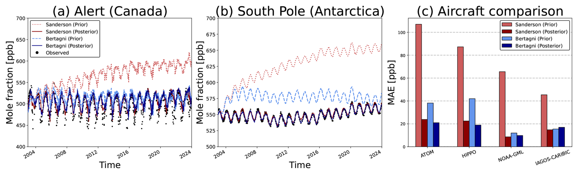
Figure 4Time series of observed (black dots) and simulated (coloured lines) H2 mole fractions at ALT (a) and SPO (b). Dotted and dashed lines show simulations before optimisation (prior), solid lines show simulations after optimisation (posterior). Red indicates Sanderson inversion, blue indicates Bertagni inversion. Panel (c) shows the prior and posterior mean absolute error (MAE), quantifying how well our simulated mole fractions match independent aircraft measurements from four campaigns. Here, the bars are ordered from left to right as Sanderson prior, Sanderson posterior, Bertagni prior, and Bertagni posterior for each campaign.
3.2 Inversions
3.2.1 Evaluation with surface and aircraft observations
Our detailed inversions substantially improve the agreement between simulated and observed H2 mole fractions used in the inversions. Globally, the mean residual across all sites decreases from 69.6 (prior) to −0.8 ppb (posterior) in the Sanderson inversion, and from 11.0 (prior) to −0.7 ppb (posterior) in the Bertagni inversion. Figure 4 shows that our inversions accurately capture the long-term growth rate and seasonal cycle at ALT (panel a) and SPO (panel b), representing the Northern and Southern Hemisphere, respectively. In addition, panel c shows that the inversions generally improve the fit to independent aircraft observations from the ATom, HIPPO, NOAA-GML, and IAGOS-CARIBIC campaigns, giving additional confidence in the results. A more detailed evaluation against aircraft measurements is provided in Table F2 in the Appendix, showing a modest latitudinal gradient in MAE, with generally lower values in the Southern Hemisphere, while altitudinal differences are less systematic and vary between campaigns.
3.2.2 The global hydrogen budget
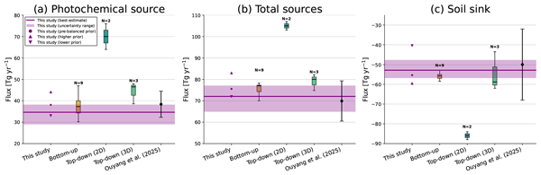
We find a global mean photochemical source of 34.6 [29.2–38.2] Tg yr−1 and a soil sink of 52.8 [47.8–56.7] Tg yr−1 for the period 2003–2023 (Table 2). Here, the central values represent the mean of our best-estimate Sanderson and Bertagni inversions (hereafter referred to as the “posterior”), and the bracketed values denote the posterior error range derived in Appendix D. Figure 5 shows that our posterior photochemical source is lower than most previous estimates (12 of 15 studies) but remains within the one-standard-deviation range given by Ouyang et al. (2025). It also shows that our posterior soil sink agrees well with most previous studies and is close to the Ouyang et al. (2025) ensemble mean. However, our posterior error range is much narrower than their soil sink one-standard-deviation range (32–68 Tg yr−1), despite covering a broad range of inversion parameters.
Ouyang et al. (2025)Table 2Optimised global H2 budget for 2003–2023 based on the mean of the best-estimate inversions using the Sanderson and Bertagni soil sink schemes. Bracketed values indicate posterior error ranges for the optimised photochemical source and soil sink, and variability across inversion experiments for the non-optimised photochemical sink (see Appendix D). Literature values are shown for comparison, noting differences in analysis periods.
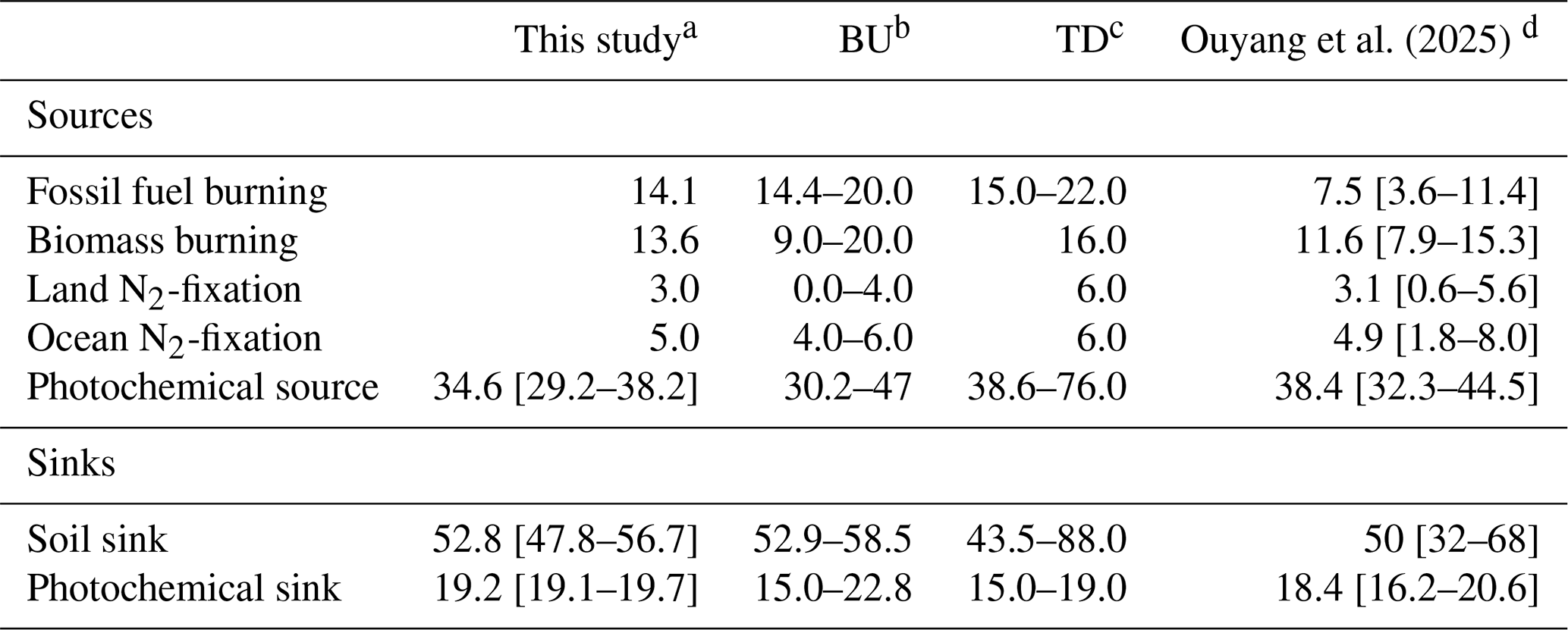
a Includes stratospheric fixing term, with mean magnitude of 3.3 Tg yr−1 (Sanderson) and 0.2 Tg yr−1 (Bertagni) over 2003–2023. b Bottom-up studies (Novelli et al., 1999; Hauglustaine and Ehhalt, 2002; Sanderson et al., 2003; Price et al., 2007; Yashiro et al., 2011; Pieterse et al., 2011, 2013; Paulot et al., 2021; Sand et al., 2023). c Top-down studies using 2D (Rhee et al., 2006; Xiao et al., 2007) and 3D models (Pison et al., 2009; Bousquet et al., 2011; Yver et al., 2011). d Recent key bottom-up study. First value denotes ensemble mean; brackets denote ±1 standard deviation.
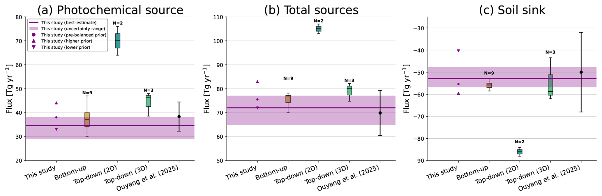
Figure 5Comparison of our fluxes with previous studies. Purple dots and triangles indicate the mean of our pre-balanced priors and alternative priors (Sanderson and Bertagni), respectively (see Sect. 3.1). Horizontal purple lines with shading show our posterior and posterior error range as derived in Appendix D. Previous studies are summarised in box plots grouped by methodological approach (see Table 2), with N denoting the number of studies in each group and whiskers extending to 1.5 IQR. Estimates from Ouyang et al. (2025) are shown as black circles with ±1 standard deviation whiskers.
3.2.3 Spatial variability
We find a high degree of consistency between the posterior-prior flux corrections applied in the Sanderson and Bertagni inversions. For the soil sink, both inversions infer weaker uptake in the Northern Hemisphere mid-latitudes and stronger uptake in the tropics compared to their priors. This reflects reduced uptake in the RECCAP2 (REgional Carbon Cycle Assessment and Processes Phase 2; Ciais et al., 2022) regions of Europe, North America, East Asia, and Russia, and increased uptake in South America, Africa, and Southeast Asia (see Appendix Figs. F2, F3, F4, F5). Figure 6 shows that relative to the Ouyang et al. (2025) ensemble mean, our posterior soil sink is roughly 45 % and 70 % stronger in South America and Russia and 45 % and 35 % weaker in the Middle East and Oceania, respectively. For the non-isoprene H2 source, both inversions yield an increase in the Northern Hemisphere (15.7 Tg yr−1 Sanderson; 15.9 Tg yr−1 Bertagni, up from 15.4 Tg yr−1) and a decrease in the Southern Hemisphere (10.9 Tg yr−1 Sanderson; 10.8 Tg yr−1 Bertagni, down from 11.8 Tg yr−1) relative to the prior. This corresponds to larger sources over Europe, North America, East Asia, and the Middle East, and smaller sources over South America and Oceania (Appendix Figs. F2, F3, F4, F5). For the isoprene H2 source, both inversions infer a consistent decrease across latitudes, with the largest reductions in the Southern Hemisphere (4.7 Tg yr−1 Sanderson; 5.0 Tg yr−1 Bertagni, down from 7.0 Tg yr−1).
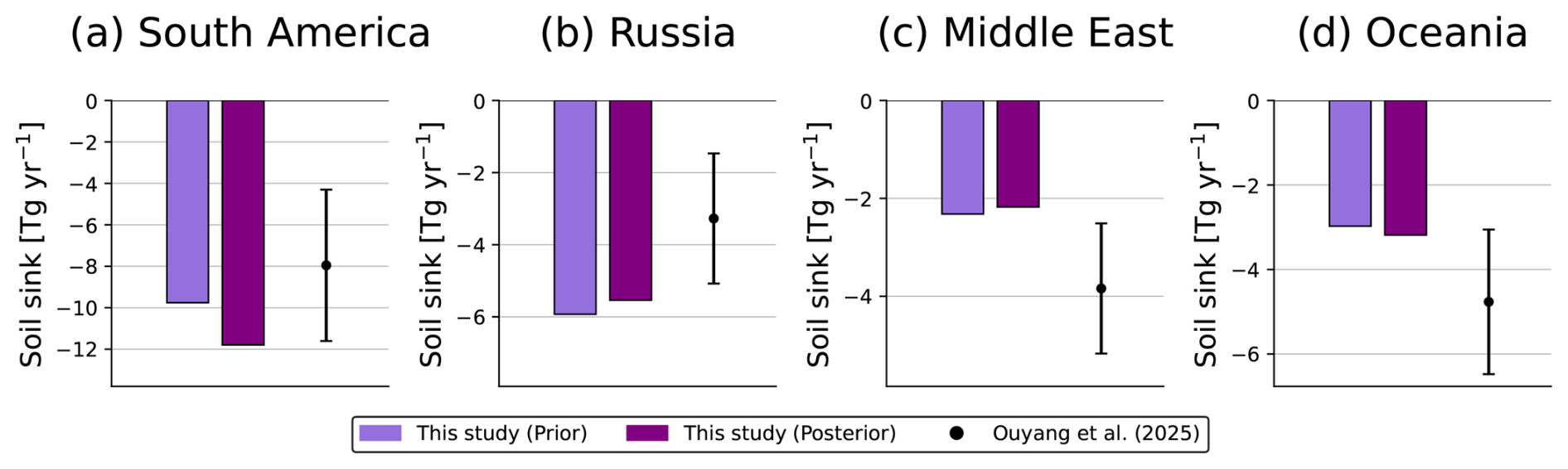
Figure 6Soil sink fluxes (2003–2023 mean) for four selected RECCAP2 regions. Light bars show the prior and dark bars the posterior, taken as the mean of the Sanderson and Bertagni inversions. Black dots with whiskers show the ensemble mean and one standard deviation range from Ouyang et al. (2025).
3.2.4 Long-term growth rate of atmospheric hydrogen
Figures 7a and 7b show the observed annual H2 growth rate from 2003–2023 (grey bars) at SPO and MLO, alongside the simulated posterior growth rate (purple bars). The record exhibits three distinct stages, most clearly at SPO: a moderate growth rate from 2003–2008, a decline from 2008–2016, and a subsequent increase after 2016. Our prior simulations do not adequately capture this temporal evolution, most notably failing to reproduce the pronounced increase in H2 after 2016 (Fig. 4). The prior biomass burning emissions (GFED5) partly explain the decline in growth rate after 2008 (Fig. 7c), whereas the prior fossil fuel burning source (Fig. 7d) and prior isoprene H2 source (Fig. 7e; dotted grey line) remain relatively constant over time. The prior non-isoprene H2 source (Fig. 7f; dotted grey line) contributes to the increase after 2016, reflecting the increasing global CH4 mole fractions in this period. This contribution is, however, partly offset by a strengthening prior soil sink (Fig. 7g; dotted grey line).
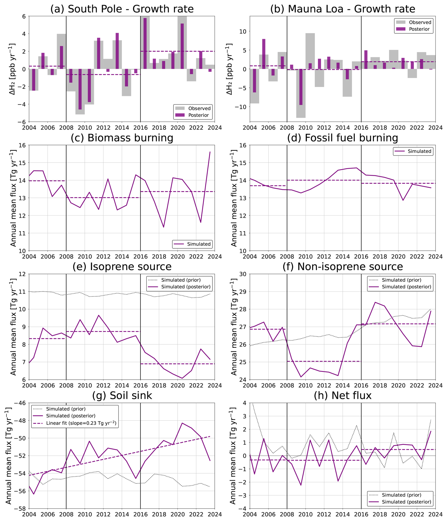
Figure 7Observed and simulated posterior annual growth rates at SPO (a) and MLO (b). Remaining panels show global annual fluxes for (c) biomass burning, (d) fossil fuel burning, (e) isoprene H2 source, (f) non-isoprene H2 source, (g) soil sink, and (h) net sources and sinks. The vertical lines delineate three periods (2003–2008, 2008–2016, 2016–2024) that characterise the observed H2 growth rate.
In the posterior, the fit to the growth rate is primarily improved by adjusting the non-isoprene H2 source (Fig. 7f), consistent with the hypothesis of Ouyang et al. (2025) that CH4-driven photochemical production is a dominant control on the atmospheric H2 growth rate. The posterior isoprene H2 source instead decreases after 2016 (Fig. 7e), but this decrease is smaller than the increase in the non-isoprene source, resulting in a net increase in posterior photochemical H2 sources. Crucially, both inversions also infer a weakening global soil sink over the last two decades, at an average rate of 0.23 Tg yr−2 (Sanderson: 0.26; Bertagni: 0.20 Tg yr−2). This result is noteworthy because a larger increase in the posterior non-isoprene source than inferred here could also have explained the observed increase in H2 growth after 2016. Instead, both inversions consistently infer a weakening soil sink, despite the increasing soil sink in their respective priors. This suggests that environmental limitations on soil uptake have strengthened over time, a change not captured by either prior deposition scheme. Given the theoretical temperature optimum of roughly 30 °C for microbial activity (Smith-Downey et al., 2006; Ehhalt and Rohrer, 2011), we consider a temperature-driven explanation less likely in light of the observed climate warming. Changes in soil moisture or other controls on microbial activity may instead contribute to the inferred trend. This finding warrants further investigation given its potential implications for future atmospheric H2 levels under the expected increase in anthropogenic emissions during the energy transition.
3.2.5 Seasonality and Interannual variability of the soil sink
Both inversions infer an increase in the seasonal amplitude of the H2 soil sink, together with a shift towards a later seasonal maximum in uptake relative to the priors. The mean seasonal range of the monthly soil sink over 2003–2023 increases in all RECCAP2 regions except Europe in the Sanderson inversion and the Middle East in the Bertagni inversion (Appendix Table F3 and Fig. F5), with the largest increases in South America, Africa, Russia, and North America. In South America, the seasonal range increases from 3.3 to 8.4 Tg yr−1 (Sanderson) and from 2.1 to 5.5 Tg yr−1 (Bertagni), in Africa from 1.2 to 6.0 and from 2.5 to 4.7 Tg yr−1, respectively, in Russia from 6.5 to 9.0 Tg yr−1 and from 7.4 to 10.3 Tg yr−1, and in North America from 5.4 to 8.1 and from 6.2 to 7.4 Tg yr−1. The strongest shifts in seasonal timing occur in Asia, particularly South Asia, East Asia, and Southeast Asia. Across all RECCAP2 regions, maximum uptake occurs 25.0 d later on average in the Sanderson posterior and 28.3 d later in the Bertagni posterior. We compare our inferred soil sink seasonality with independent estimates by Stone et al. (2026) and Tardito Chaudhri and Stevenson (2025) in Appendix B. We find excellent agreement with Stone et al. (2026) in both seasonal range and timing, but poor agreement with Tardito Chaudhri and Stevenson (2025), likely due to substantial methodological differences between our studies.
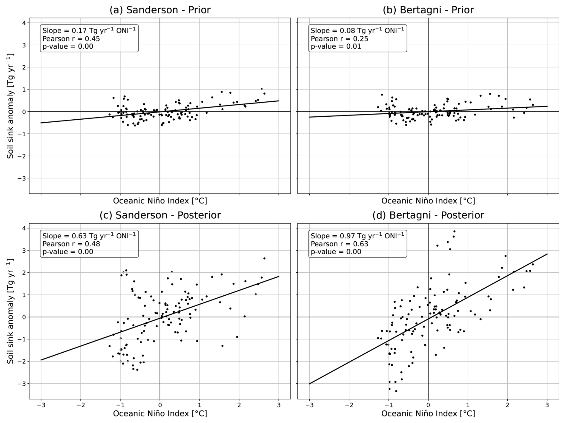
Figure 8Monthly soil sink flux anomalies for tropical South America (RECCAP2 region), defined relative to a month-specific climatology over the final 10 years of the inversions (2014–2024), plotted against the Oceanic Niño Index (Barnston et al., 1997). Left panels correspond to the Sanderson inversion, right panels to the Bertagni inversion.
Our inversions also show a clear sensitivity of the soil sink to the El Niño–Southern Oscillation (ENSO). This response is strongest in tropical South America (Fig. 8) but remains statistically significant globally, including weaker but significant correlations for several other regions (Table F4 in the Appendix). We hypothesise that ENSO primarily influences the soil sink through soil moisture. According to Bertagni et al. (2021), in most regions, including tropical South America, the soil sink is dominantly diffusion-limited (i.e., too wet). Therefore, the drier conditions in the Amazon associated with El Niño may temporarily reduce the diffusive barrier and increase the soil sink, whereas wetter conditions during La Niña increase the diffusive barrier and dampen the soil sink. This could explain the upper right and lower left quadrants of Fig. 8, respectively. Notably, this ENSO–soil sink relationship was only very weakly present in the priors, but emerges much more clearly in the posteriors, highlighting the additional information provided by the atmospheric constraints.
4.1 Uncertainty and potential aliasing in the inferred H2 budget
We have relatively high confidence in our inferred soil sink, supported by the use of observationally constrained OH fields and the agreement of our estimated photochemical sink with other bottom-up estimates. To estimate the photochemical sink, we used OH fields from the CAMS EAC4 reanalysis, which provides globally consistent atmospheric composition fields constrained by satellite observations of O3, CO, NO2, and aerosol optical depth, alongside meteorological observations (Inness et al., 2019). Our resulting photochemical sink of 19.2 [19.1–19.7] Tg yr−1 falls within the range of other bottom-up estimates (15.0–22.8 Tg yr−1; see Table 2) and is very close to the mean estimate of 18.4 [16.2–20.6] Tg yr−1 reported by Ouyang et al. (2025). We note that Sand et al. (2023) reported a higher photochemical sink of 25 [22–30] Tg yr−1 from an ensemble of global three-dimensional atmospheric chemistry models. However, Yang et al. (2025) showed that these models tend to overestimate OH, which explains the higher estimates of the photochemical H2 sink. Supporting this, Sand et al. (2023) report CH4 lifetimes due to OH oxidation of 8.0 [6.9–9.2] years across their ensemble of models, substantially shorter than the lifetime of 11.2 ± 1.3 years inferred from observations (Prather et al., 2012).
We note that our reported range of 19.2 [19.1–19.7] Tg yr−1 represents variability in the mean photochemical sink over 2003–2023 across our inversion experiments, rather than an uncertainty estimate that includes OH uncertainty. This variability arises from differences in the posterior photochemical source, posterior soil sink, and spatiotemporal distribution of posterior mole fractions, as the photochemical sink is not directly optimised in our inversions. We are aware that the range in our photochemical H2 sink is narrow relative to the broader uncertainties in global OH distributions, which partly reflects our use of the same CAMS EAC4 OH fields in all experiments. Therefore, to illustrate the potential implications of OH-field uncertainties, we consider a hypothetical 20 % bias in OH fields. Under a first-order approximation, assuming full compensation in the inversion by an opposite change in the soil sink, this would result in a change in our posterior soil sink of approximately 3.9 Tg yr−1. This change is relatively small compared to the posterior error range on the soil sink (47.8–56.7 Tg yr−1), supporting our conclusion that the inferred soil sink is relatively robust against 20 % variations in OH. Changes in the north–south gradient of OH (Naik et al., 2013; Naus et al., 2021) or in its interannual variations (Patra et al., 2021) would likely affect the photochemical sink and hence soil sink patterns within this global constraint, but these effects are not quantified in our study.
We are also confident in our inferred total sources, although constraining the photochemical source is more challenging. This arises from the fact that several other sources in the hydrogen budget are prescribed in our inversions rather than optimised, introducing a potential for aliasing, whereby biases in these prescribed terms are compensated by adjustments in the posterior photochemical source or soil sink. For example, the three-stage pattern in our posterior photochemical source could also partly reflect a systematic underestimation of biomass burning H2 emissions in the GFED5 prior, which showed a similar temporal structure. However, this is unlikely to fully explain our inferred trend, as GFED5 H2 emissions already lie at the upper end of current literature estimates (Ouyang et al., 2025). Similarly, sources not included in our model provide an additional pathway for aliasing. For example, geological sources and leakage-related industrial emissions were omitted due to the lack of robust emission inventories and their expected small magnitude (Ouyang et al., 2025). If sufficiently large and increasing over time, these fluxes could in principle contribute to the inferred weakening of the global soil sink. This is unlikely for geological sources, for which no clear mechanisms support a sustained long-term increase. Industrial emissions provide a more plausible pathway, as global hydrogen demand increased from 52.5 Tg in 2000 (IEA, 2019) to 95 Tg in 2023 (IEA, 2023), implying an approximate doubling of emissions under constant loss rates. However, fully explaining our inferred soil sink trend (4.8 Tg yr−1 reduction over 2003–2023) would require losses of approximately 11.3 % across the hydrogen supply chain. This lies at the upper end of literature estimates (∼10 %) and well above current best estimates (1.3 %; Trapani et al., 2025), suggesting that industrial emissions may contribute but are unlikely to fully explain our inferred trend.
A possible misattribution of sources and sinks of H2 could be evaluated by propagating our H2 fluxes into simulated hydrogen deuteride (HD) abundances, following an approach similar to Pieterse (2013). While the photochemical source has limited isotopic leverage, the soil sink enriches the atmosphere in HD (Chen et al., 2015). We therefore expect that a decreasing soil sink would contribute to declining global HD levels over time. In the case of a strong increase in industrial or geological emissions, we also expect declining HD levels, since these sources are strongly isotopically depleted (Gibson et al., 2024). However, no HD observations have been published over the past 15 years, meaning this cannot be tested. In addition, other sources and sinks with greater isotopic fractionation have likely evolved in recent decades, as well as their corresponding source signatures. For example, advances in engine technology have likely altered both the H2 : CO emission ratio used to infer fossil fuel burning H2 emissions from CO emissions and the isotopic signature of the resulting H2 (Vollmer et al., 2010); however, such changes remain poorly characterised.
Our inverse problem is further complicated by the opposing signs and substantial spatial overlap of the soil sink and photochemical source (particularly the isoprene-related partition), both of which peak in tropical regions, leading to strong posterior correlations between these flux components (see Appendix E). Flux separability is further complicated by the low observational density in these regions. As recently noted by Tardito Chaudhri and Stevenson (2025), local process-based measurements are crucial for improving understanding of tropical soil H2 fluxes. We further emphasise the need for expanded atmospheric mole fraction observations to constrain future inverse modelling studies, as these regions remain among the least observed globally. A challenge specific to the photochemical source is its three-dimensional nature, making it more difficult to constrain using surface observations alone (Bousquet et al., 2011). Despite this, we consider multi-species inversions a promising approach to better quantify this term, given the strong chemical coupling between H2, CH2O, CO, and OH. Pison et al. (2009) applied such a framework, however we identify a clear opportunity to revisit it in light of nearly two decades of satellite observations of CO and CH2O since then.
4.2 Causes of an overestimated prior photochemical H2 source
We found a significantly lower posterior photochemical H2 source compared to the prior derived from the full-chemistry simulation. This reduction occurred mainly in the pre-optimisation with global scaling factors (Sect. 3.1), but also in the subsequent detailed inversions (Sect. 3.2). Comparison with ATom aircraft observations (Appendix A) shows that the inversions have likely compensated for an overestimation of the CH2O photolysis rate constant through the molecular channel (i.e., the H2-producing pathway), with the magnitude of this overestimation increasing towards the surface. In addition, the inversions likely corrected for an overestimation of CH2O mole fractions over land, particularly in the lower atmosphere. The overestimation of the molecular-channel photolysis rate constant is possibly related to its 30 % increase in the updated CBM4 (Carbon Bond v4) and subsequent CB05 mechanism relative to the original CBM4, introduced to improve simulated CO, CH4, and O3 (Williams and Van Noije, 2008). However, the impact of this enhancement of the H2-producing photolysis channel on simulated H2 was not evaluated in this study.
4.3 Implications of ENSO-driven soil uptake variability for other trace gases
Our inferred H2 soil sink sensitivity to ENSO likely extends to other trace gases such as CH4, CO, N2O and COS, since their uptake efficiency also depends on gas diffusion through the soil pore network. When soils become water-saturated, diffusion is reduced as pores fill with water, limiting access to microbial or chemical sinks. Field measurements support this theory, as Aronson et al. (2019) conducted soil chamber measurements in a tropical forest in Costa Rica and showed that ENSO cycles influence biogenic CH4 fluxes through soil moisture changes, with CH4 consumption highest during the driest phase of El Niño and reduced uptake during La Niña and wetter conditions. These results align with our findings and support an ENSO-driven modulation of the H2 soil sink in tropical regions, with similar moisture-driven mechanisms proposed.
In this study, we performed atmospheric inversions of H2 using the TM5 chemical transport model to derive a spatiotemporally resolved budget over the period 2003–2023. Using this approach, we infer a global mean H2 soil sink of 52.8 [47.8–56.7] Tg yr−1 and a global photochemical H2 source of 34.6 [29.2–38.2] Tg yr−1 over 2003–2023. Notably, our soil sink posterior error range is substantially narrower than the one standard deviation range reported by Ouyang et al. (2025). We also infer a soil sink that is 45 % and 35 % weaker in the Middle East and Oceania and 45 % and 70 % stronger in South America and Russia, respectively, relative to Ouyang et al. (2025). Our results further suggest that variability in atmospheric H2 growth rates between 2003 and 2023 was primarily driven by changes in the non-isoprene photochemical source, consistent with the recent hypothesis of Ouyang et al. (2025) that CH4-driven photochemical production is a dominant control on the atmospheric H2 growth rate. Additionally, our results show a weakening of the global soil sink at a mean rate of 0.23 Tg yr−2 over this period. We recommend further investigation into this, given the potential implications for future atmospheric H2 levels in light of the projected increase in anthropogenic emissions during the ongoing energy transition. Finally, our results show a clear sensitivity of the H2 soil sink to the El Niño–Southern Oscillation, strongest over diffusion-limited soils in tropical South America, with increased uptake during drier El Niño conditions and reduced uptake during wetter La Niña conditions. This sensitivity may extend to other tracers, such as CH4, CO, N2O, and COS, given that their uptake is also dependent on diffusion through the soil pore network.
To further improve quantification of the global hydrogen budget, progress is needed along two complementary directions: improved process understanding to refine prior flux estimates and expanded observational constraints for future inverse modelling studies. For process understanding, additional field measurements of the soil sink across a broad range of environments are key, with particular emphasis on tropical regions, as noted by Tardito Chaudhri and Stevenson (2025). For observational constraints, expanding H2 mole fraction measurements in the tropics should be a priority, given the large fluxes and sparse observational coverage in these regions. Measurements and simulations of HD may provide additional constraints on the global H2 budget, as demonstrated by Pieterse et al. (2013). However, the potential of HD is limited by the absence of observations over the past 15 years, as well as limited progress in constraining source signatures and fractionation factors. Finally, for the photochemical H2 source, we consider multi-species inversions a promising approach given the strong chemical coupling between H2, CH2O, CO, and OH. Pison et al. (2009) applied such a framework, and we identify a clear opportunity to revisit it in light of nearly two decades of satellite observations of CO and CH2O since then.
To assess whether our prior photochemical H2 source fields provide a reasonable starting point for the inversions, we evaluate simulated CH2O mole fractions and the photolysis rate constant () against aircraft observations from the ATom campaign (Hall et al., 2018; Hanisco et al., 2019; Wofsy et al., 2021). The latter refers to the molecular photolysis channel of CH2O, which is the H2-producing pathway.
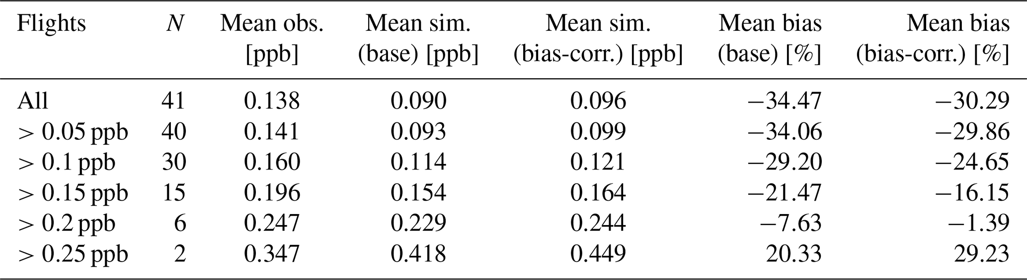
Figure A1 shows that our simulations adequately capture most of the observed large-scale variability in CH2O, including enhanced mole fractions over polluted continental regions. The simulations reproduce the near-surface land-ocean gradient of approximately 1 ppb over North America and the increase toward the surface due to enhanced precursor emissions. Across all flights (N=41), the simulated and observed latitudinal and vertical gradients agree relatively well (Fig. A2), although our simulations show a general negative bias. The mean CH2O mole fraction across all ATom observations was 0.138 ppb, compared to 0.090 ppb in our simulations, yielding a mean bias of −0.048 ppb (−34.5 %; Table A1). For the six flights with mean observed CH2O mole fractions above 0.2 ppb, however, the bias is reduced to −0.018 ppb (−7.6 %). Five of these flights sampled tropical ocean regions, where enhanced CH4 oxidation likely contributed to elevated CH2O levels. The sixth flight sampled continental air over the United States, where greater OH availability, together with anthropogenic and biogenic VOC emissions, likely contributed to the elevated CH2O levels.
Figure A3 shows that our hourly simulated values display a mean bias of +7.4 % across all altitudes relative to the ATom observations. However, this bias increases towards the surface, with values of +23.5 % between 0–2 km and +17.1 % between 2–4 km altitude. Besides this vertical structure, the bias is relatively uniform across latitudes, except between 60 and 90° S, although this region contains few ATom observations and is relatively unimportant for H2 production given that both and CH2O mole fractions are low here. Based on the identified vertical bias structure, we calculated correction factors for for each model vertical layer and reran the full-chemistry simulation for the 2016–2018 period. As expected, the lower values resulted in slightly larger simulated CH2O mole fractions (Figs. A1 and A2). Applying this correction reduced the annual mean photochemical H2 source from 55.0 to 50.3 Tg yr−1 in 2016–2017, still substantially above our posterior estimate of 36.0 Tg yr−1 obtained after the global scaling in Sect. 3.1 and subsequent detailed inversions in Sect. 3.2.
We hypothesize that the remaining difference is related to an overestimation of CH2O in regions important for photochemical H2 production. Evidence for such a bias is provided by the flight over the continental United States (Fig. A1), where simulated CH2O exceeds observations in the lower troposphere, where both CH2O concentrations and photochemical H2 production are high. This regional bias is not apparent in the overall ATom mean because ATom predominantly sampled remote oceanic and background conditions, where CH2O concentrations and photochemical H2 production are lower. The ATom mean therefore does not necessarily represent CH2O biases in regions that contribute most strongly to the global photochemical H2 source. While the bias can be directly corrected using the observational constraint presented here, addressing the CH2O bias would require changes to precursor emissions or the chemical mechanism and is beyond the scope of this study.
Since the correction reduced the prior photochemical H2 source by approximately 3 Tg yr−1 after applying the global scaling factor of 0.7 from Sect. 3.1, we assessed its impact on posterior fluxes. We performed two inversions for 2016–2018 using photochemical H2 source fields with and without the correction. The uncorrected case used the original source fields from the full inversions but was rerun over 2016–2018 to ensure a consistent comparison, excluding observations outside this period that influenced the original inversion through the temporal correlations described in Appendix C1. For 2016–2017, applying the correction changed the posterior fluxes from 50.0 to 48.3 Tg yr−1 for the soil sink, from 27.8 to 26.7 Tg yr−1 for the non-isoprene H2 source, and from 8.2 to 7.5 Tg yr−1 for the isoprene H2 source. Although these changes are not negligible, they remain well within the uncertainty ranges established in Appendix D. Therefore, we do not deem it necessary to rerun all inversions with the bias-corrected photochemical sources.
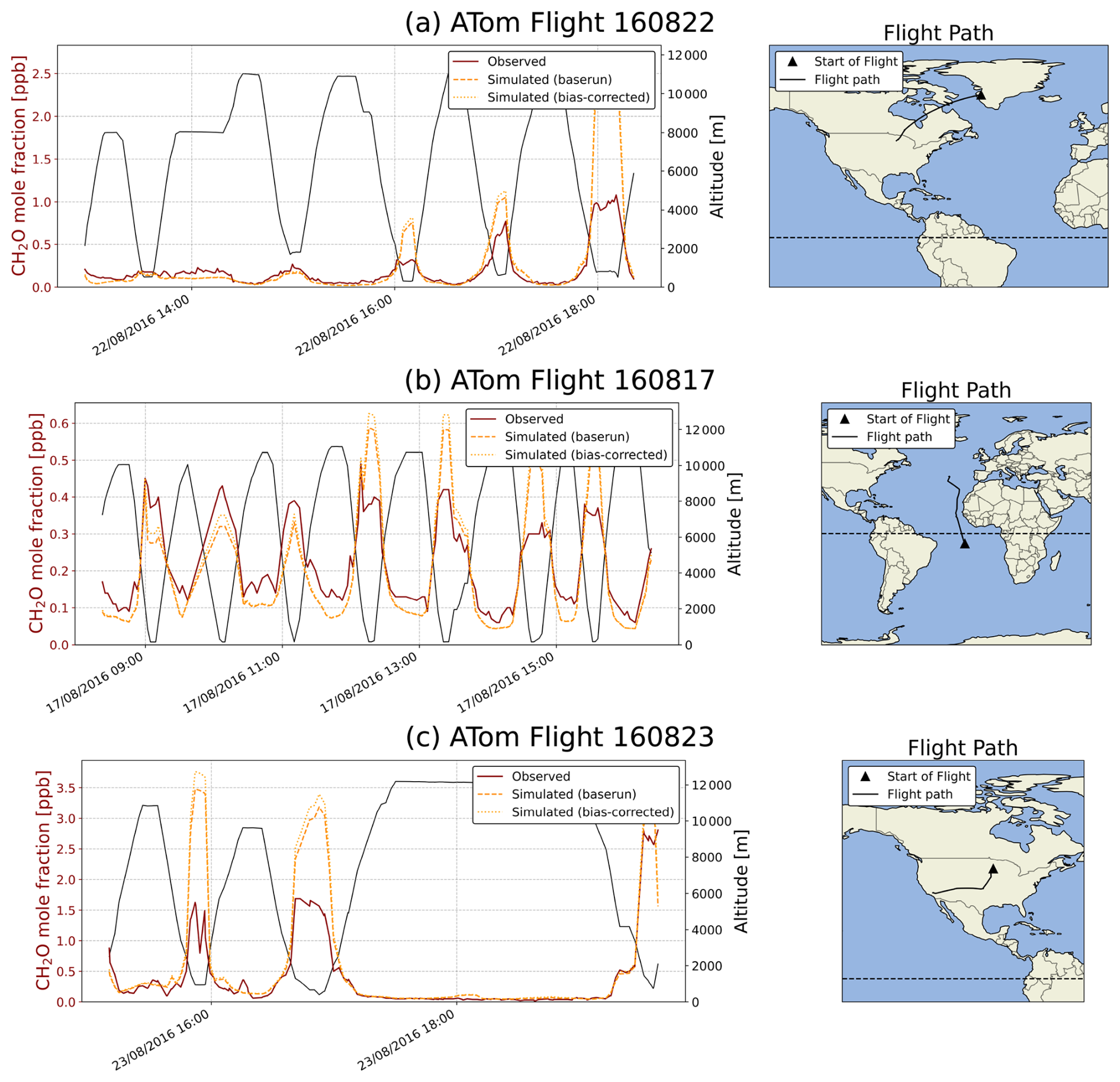
Figure A1Observed and simulated CH2O mole fractions for three ATom flights: (a) 160 822 (mean bias: base run =36.2 %, bias-corrected run =47.3 %), (b) 160 817 (mean bias: base run , bias-corrected run =0.3 %), and (c) 160 823 (mean bias: base run =44.5 %, bias-corrected run =55.2 %). Left axis: CH2O mole fraction; right axis: altitude along flight track.
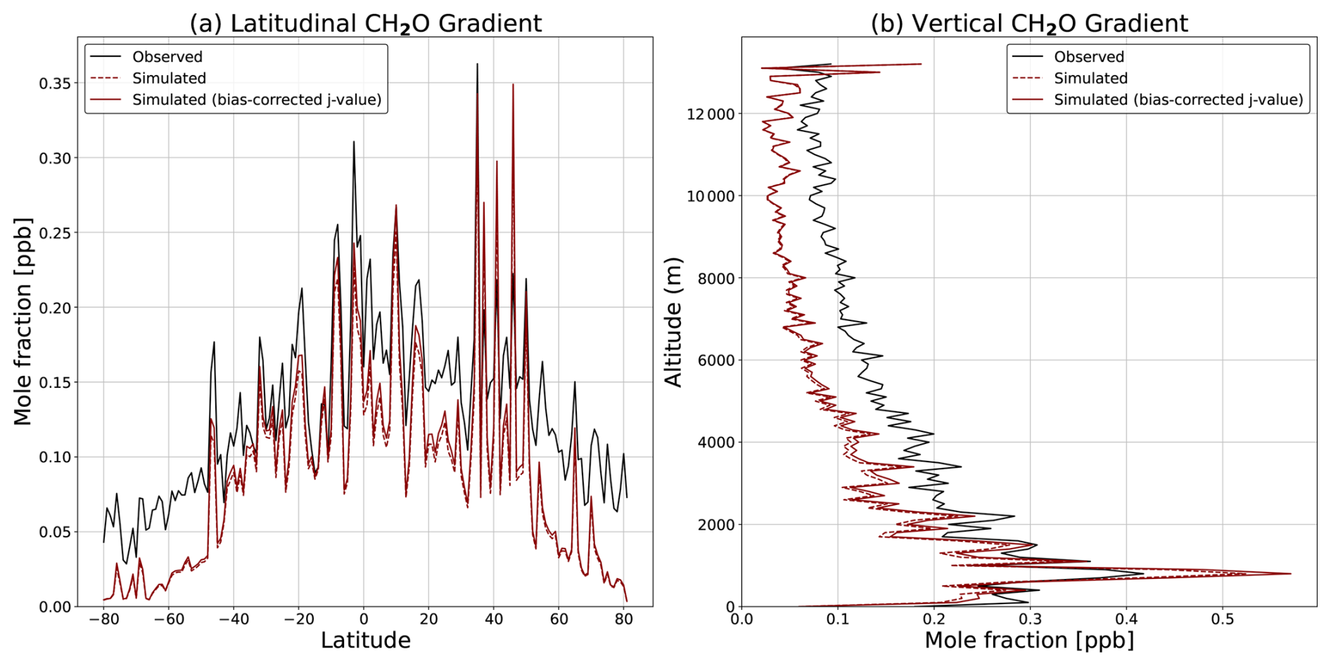
Figure A2Latitudinal and vertical gradients in observed and simulated CH2O mole fractions for the ATom flights. Results are shown for simulations with and without bias correction.
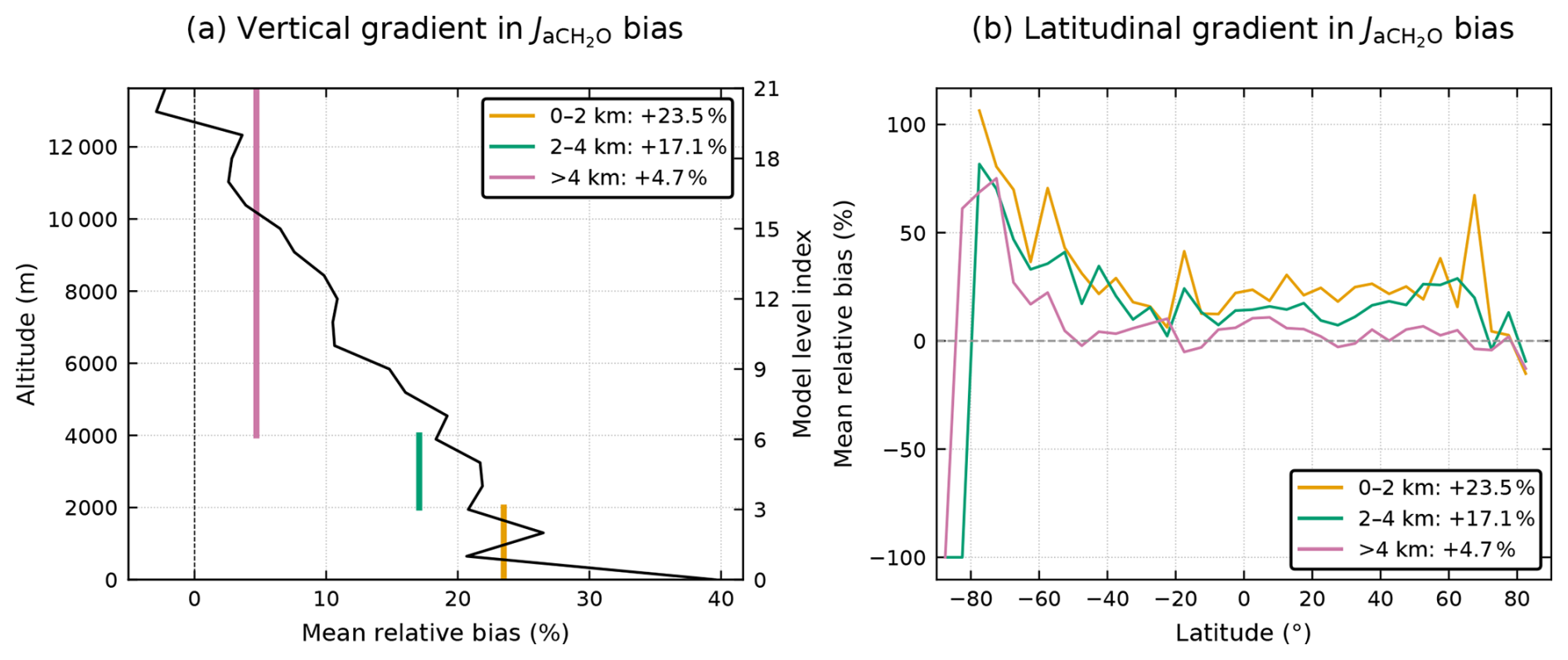
Figure A3Vertical and latitudinal gradient in simulated bias in the photolysis rate constant for the photolysis of CH2O through the molecular channel ().
Table A1Summary statistics of observed and simulated CH2O mole fractions from ATom flights for all flights and subsets with increasing minimum observed CH2O. The table compares observations with the baserun and bias-corrected simulations, reporting the mean simulated mole fractions and the corresponding mean biases relative to observations.
We compare our inferred H2 sink seasonality with the independent estimates of Stone et al. (2026) and Tardito Chaudhri and Stevenson (2025). For this, we calculated the seasonal range and the timing of maximum uptake of our simulated soil sink using the NOAA CCGCRV curve-fitting package (Thoning et al., 1989; NOAA Global Monitoring Laboratory, 2026).
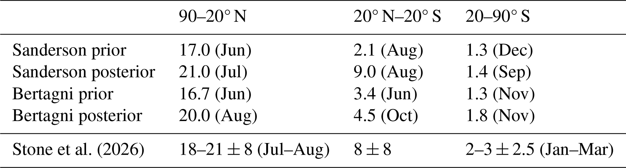
Stone et al. (2026) used HFC-152a observations in a Bayesian three-box inversion to jointly constrain OH seasonality and infer the H2 soil-sink cycle for the Northern Hemisphere (90–20° N), tropics (20° N–20° S), and Southern Hemisphere (20–90° S). We find excellent agreement in seasonal range and timing, particularly in the Northern Hemisphere (Table B1). Here, our posterior seasonal ranges of 21.0 and 20.0 Tg yr−1 for Sanderson and Bertagni closely match their estimate of 18–21 ± 8 Tg yr−1, and our posterior soil sink peaks in July and August, respectively, coinciding with the July–August peak reported by Stone et al. (2026). In the tropics, our Sanderson posterior seasonal range of 9.0 Tg yr−1 agrees very well with their estimate of 8 ± 8 Tg yr−1, while the Bertagni posterior of 4.5 Tg yr−1 still falls well within their reported uncertainty range. Stone et al. (2026) find substantial variation in the timing of maximum uptake across their four experiments, with peaks in January, April, and August. Our inferred maxima in August and October are in good agreement with two of their four experiments, which showed an August maximum. In the Southern Hemisphere, our posterior seasonal ranges of 1.4 and 1.8 Tg yr−1 both fall within their reported range of 2–3 ± 2.5 Tg yr−1. Interestingly, our Southern Hemisphere soil sink peaks in November, consistent with Bousquet et al. (2011) and Xiao et al. (2007), whereas Stone et al. (2026) find a January–March maximum, closer to the February peak reported by Rhee et al. (2006).
Stone et al. (2026) also constrained the seasonality of chemical loss by OH. In the Northern Hemisphere, our posterior seasonal ranges of 8.8 and 8.9 Tg yr−1 for Sanderson and Bertagni closely match their estimate of 8 ± 1 Tg yr−1, and both inversions peak in July, consistent with their June–July maximum. In the tropics, our chemical loss term is relatively constant throughout the year, yielding a seasonal range of only 1.1 Tg yr−1, which falls outside their reported range of 4 ± 2.5 Tg yr−1, with maximum loss occurring in September compared with their February–March maximum. This larger discrepancy in the tropics may reflect differences in the seasonality of photochemical production and other H2 sources between the two approaches. In the Southern Hemisphere, both inversions yield a seasonal range of 4.9 Tg yr−1, lower than their estimate of 7 ± 1 Tg yr−1, while our January maximum is consistent with their December–January maximum.
Interestingly, our inferred soil-sink seasonality differs substantially from Tardito Chaudhri and Stevenson (2025), who used a zonal-mean two-dimensional model with four vertical levels to optimise H2 soil-sink seasonality in three latitude bands. In the 30° S–0° N band, our posterior seasonal ranges are 6.4 and 2.2 Tg yr−1 for Sanderson and Bertagni, respectively, compared with their substantially larger estimate of 21.9 Tg yr−1. The timing of maximum uptake also differs, occurring in September and June in our inversions, respectively, compared with May in their study. Similarly, in the 0–30° N band, our posterior seasonal ranges of 5.9 and 1.7 Tg yr−1 are lower than their estimate of 18.1 Tg yr−1, with maximum uptake occurring in March and December, respectively, compared with October. In the 30–60° N band, our seasonal ranges of 12.7 and 14.0 Tg yr−1 are again lower than their estimate of 23.1 Tg yr−1, while our maxima occur in June and May, respectively, compared with September. Thus, compared with Tardito Chaudhri and Stevenson (2025), our inversions consistently infer weaker seasonal variations and generally different timing of maximum uptake. We attribute this to the different methodological approaches used in the two studies: Tardito Chaudhri and Stevenson (2025) optimise only the soil sink using a zonal-mean transport framework, whereas we jointly optimise the soil sink and photochemical H2 source using a three-dimensional framework. Furthermore, Tardito Chaudhri and Stevenson (2025) used a smaller set of observations (i.e., only NOAA-GML data).
Stone et al. (2026)Table B1Seasonality of the soil sink in our inversions compared with Stone et al. (2026). Our fluxes are evaluated over 2010–2022 to match Stone et al. (2026). We calculate the seasonal range and timing of maximum uptake using the NOAA CCGCRV curve-fitting package (Thoning et al., 1989; NOAA Global Monitoring Laboratory, 2026). Values show the seasonal range in Tg yr−1 followed by the month of maximum sink strength. Stone et al. (2026) provide only one seasonal range value for the tropics box (from their “OH case”) and no month of maximum sink strength, since the latter varies between cases.
To determine the best-performing inversion settings, we conducted various experiments at a 6°×4° horizontal resolution with 25 vertical levels, covering 2003–2013. We used the optimal prior Bertagni soil sink and photochemical source fluxes derived in Sect. 2.4 and the settings described in Sect. 2.5 unless stated otherwise. We use an ensemble size of 150 members, which is sufficient given our chosen uncertainties for each statevector element in space and time. However, our main results in Sect. 3.2 are still obtained with 300 members to be conservative and account for potential sensitivity to random sampling, particularly since tests showed that larger uncertainties on the statevector elements increase this sensitivity.
C1 Temporal correlations
To establish robust temporal correlations, we first examined the effect of the σMOY parameter in our statevector (Table C1). This parameter describes the extent to which observations from neighbouring years influence monthly scaling, and its use is based on the assumption that a large part of the error shows seasonal behaviour. In our first experiment (A1), we use a 60-month value for the non-isoprene H2 source, assuming that CH4 mole fractions show low interannual variability. For the soil sink, we use a 36-month value, assuming that this term is more variable, but that this variability is already partly captured in our input datasets. Finally, we use a 24-month value for the isoprene H2 source, since its interannual variability is poorly understood and poorly constrained. Shorter timescales or uniform long timescales were also tested (Table C1).
Table C1Impact of the σMOY parameter, which prescribes the decay time of correlations between the same months of adjacent years (J–J, F–F, M–M, ...), on the fraction of grid cells with optimised scaling factors that reverse the sign of the prior flux.

Table C2Impacts of progressively refined MDM classes for different site categories on posterior chi-squared () at MAA (Mawson, Antarctica), MLO (Mauna Loa, Hawaii), MHD (Mace Head, Ireland), and NWR (Niwot Ridge, USA). These sites represent Deep Southern Hemisphere, Marine Boundary Layer, Mixed, and Land environments, respectively. Additionally, the fraction of grid cells with optimised scaling factors that reverse the prior flux sign is shown.
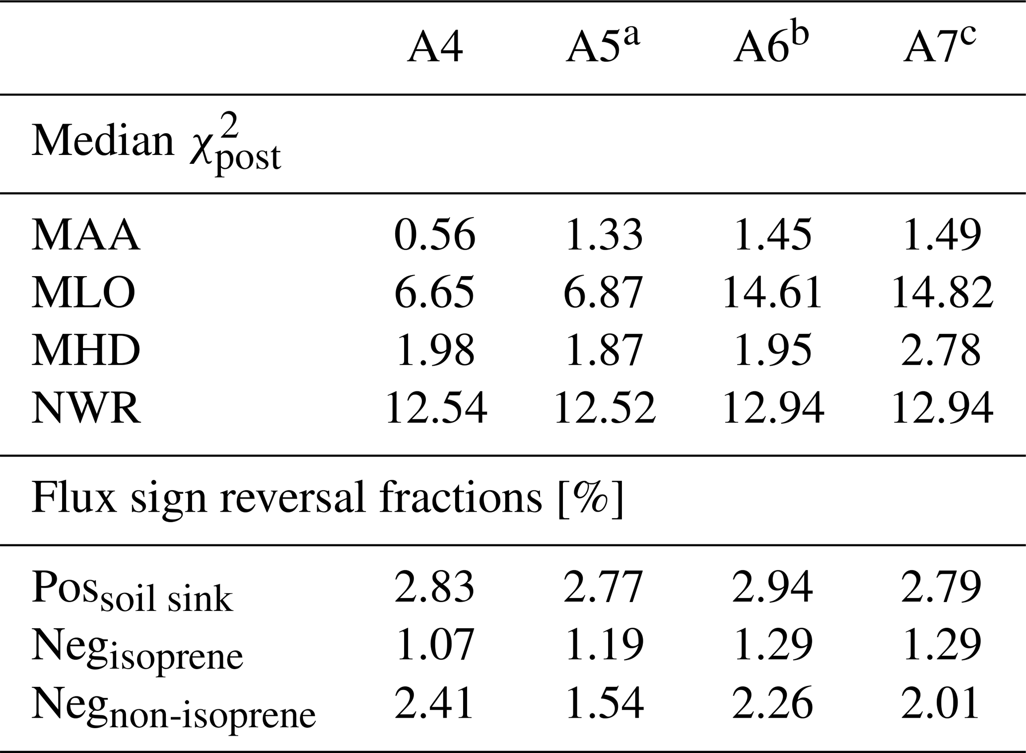
a Deep Southern Hemisphere (1.5 ppb MDM). b Deep Southern Hemisphere (1.5 ppb MDM) + Marine Boundary Layer (2.0 ppb MDM). c Deep Southern Hemisphere (1.5 ppb MDM) + Marine Boundary Layer (2.0 ppb MDM) + Mixed (2.5 ppb MDM).
We identify experiment A2 as the best-performing configuration, as it yields the most physically consistent and interpretable flux estimates, with the lowest fraction of grid cells in which the optimised scaling factors reverse the sign of the prior flux, resulting in positive soil sinks or negative photochemical sources (Table C1). This is illustrated for the South America RECCAP2 region in Fig. C1, where experiments with longer temporal correlation scales (A1 and A3) show a reduced soil sink, compensated by a smaller photochemical source (panel a). This is unlikely, as it largely arises from a more negative photochemical source (panel b) and a more positive soil sink (panel c). We also find this in other regions, including Africa and Oceania (not shown here). Experiment A2 also performs better because it has a more spatially coherent optimised soil sink and a non-isoprene H2 source, in contrast to the scattered and dipole-like patterns obtained in experiments A1 and A3. Finally, the regional fluxes of A2 show realistic interannual variability, whereas variability is strongly suppressed in A1 and A3. Based on these considerations, we adopt the σMOY values from experiment A2 for all remaining inversions.
C2 Model-data mismatch
Next, we investigated the sensitivity of the inversions to the value of the model–data mismatch (MDM). This was achieved through offline inversions, which avoided rerunning the full transport model and reduced computational costs. In the base configuration (experiment A4), a uniform MDM of 3.0 ppb was assigned to all sites. To introduce spatially varying but physically motivated uncertainties, we performed a sequence of experiments with progressively refined site classifications. In experiment A5, Deep Southern Hemisphere (Deep SH) sites were assigned a reduced MDM of 1.5 ppb to reflect their relatively low transport and representation errors (Fig. C2), while all remaining sites retained an MDM of 3.0 ppb. Experiment A6 further distinguished marine boundary layer (MBL) sites, which were assigned an intermediate MDM of 2.0 ppb in addition to the reduced MDM for Deep SH sites. Finally, in experiment A7, mixed sites were assigned an MDM of 2.5 ppb, while land sites, characterised by stronger flux heterogeneity and transport uncertainty, retained the highest MDM of 3.0 ppb. We find experiment A5 performs best, because it yields a posterior chi-squared (χ2) closest to unity at three out of four sites that we selected to represent the MDM classes (Deep SH, MBL, Mixed, and Land). Furthermore, experiment A5 produces the lowest fraction of grid cells with sign-reversing optimised scaling factors, leading to a negative non-isoprene H2 source or a positive soil sink (i.e. physically implausible fluxes), and hence we adopt its MDM classification in the remaining experiments (Table C2).
C3 Statevector element uncertainty
Lastly, we conducted offline inversion experiments by perturbing the uncertainties in our statevector elements across space and time. This was motivated by the observed relationship between the choice of these uncertainties and the occurrence of unphysical scaling factors, which could produce either a negative photochemical source or a positive soil sink (Fig. C3), even with a 300-member inversion. We found that reducing these uncertainties improved the physical consistency of the optimised fluxes while still allowing meaningful adjustments. The initial uncertainties were 15 %, 10 %, and 5 % for the soil sink, isoprene H2 source, and non-isoprene H2 source, respectively. Multiplying these values by a factor of 0.5 provided an optimum balance between minimising unphysical fluxes and maintaining meaningful spatial and temporal adjustments, as shown in Fig. C3. Another reason for choosing the factor 0.5 was that lowering it further led to increasingly large posterior residuals, as denoted by panel d. Consequently, in the main inversions, uncertainties of 7.5 %, 5 %, and 2.5 % are used for the soil sink, isoprene H2 source, and non-isoprene H2 source, respectively.
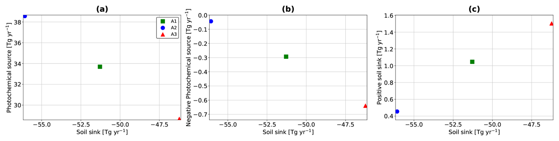
Figure C1Annual mean H2 fluxes over the South America RECCAP2 region (2003–2013) for the three σMOY experiments. Panel (a) shows the soil sink versus the photochemical source, panel (b) shows the soil sink versus the negative photochemical source, panel (c) shows the soil sink versus the positive soil sink over this region.
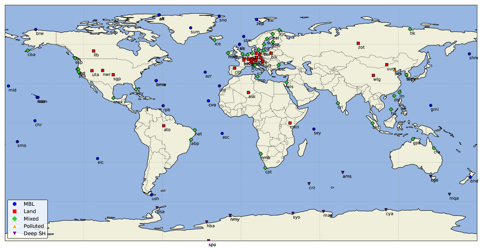
Figure C2Global distribution of H2 surface flask and in situ sampling sites used in this study. Sites are coloured according to their site classification: marine boundary layer (MBL), land, mixed, polluted, and deep Southern Hemisphere (Deep SH).
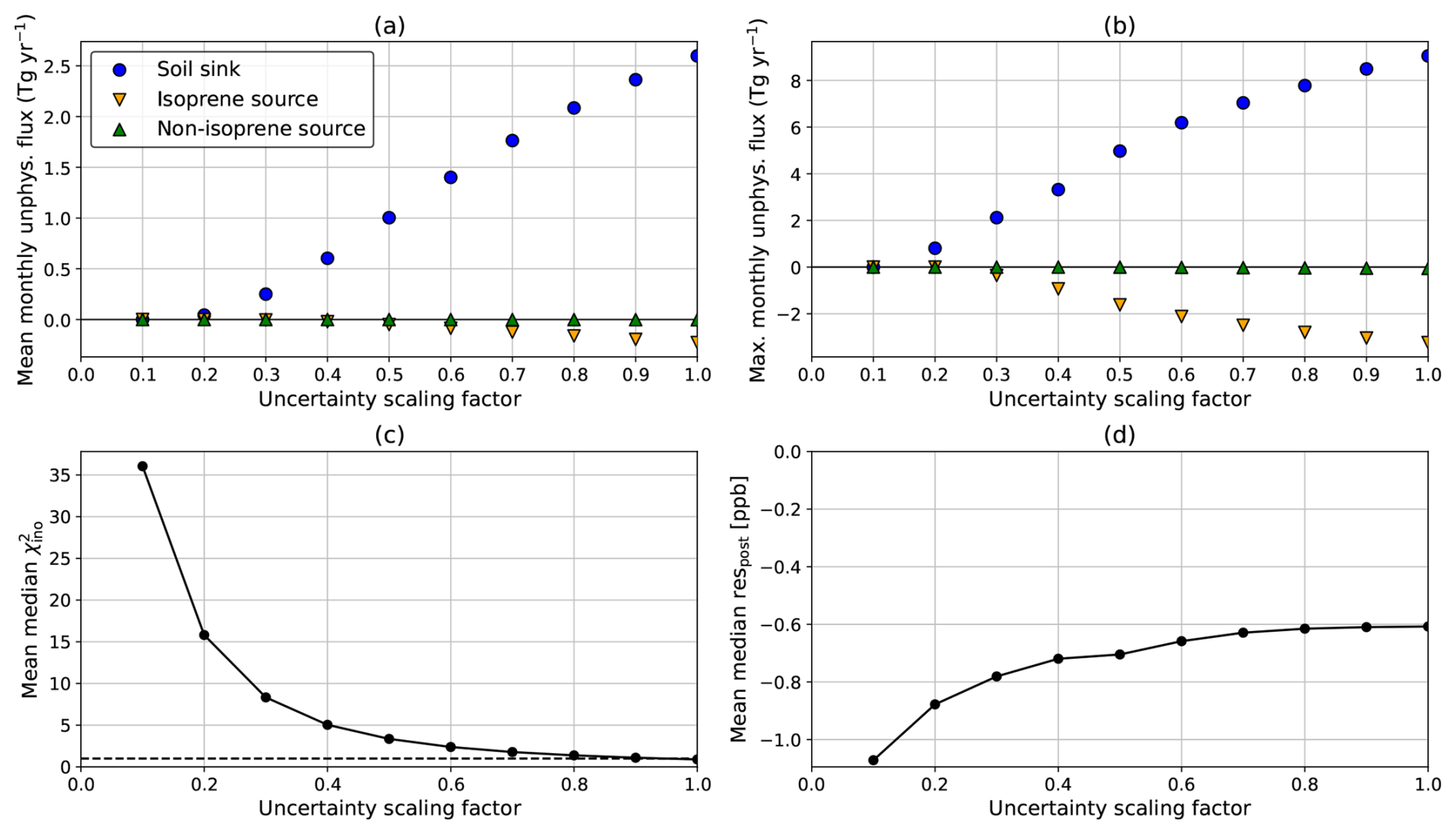
Figure C3Sensitivity of unphysical H2 fluxes and inversion performance metrics to the statevector element uncertainty scaling factor (PU). (a) Monthly mean positive soil dry deposition (sink) and negative photochemical production from isoprene and non-isoprene precursors (sources). (b) Maximum monthly values of these unphysical fluxes during the runtime (2003–2023). (c) Mean of the median innovation chi-squared () across all sites. (d) Mean of the median posterior residual across all sites.
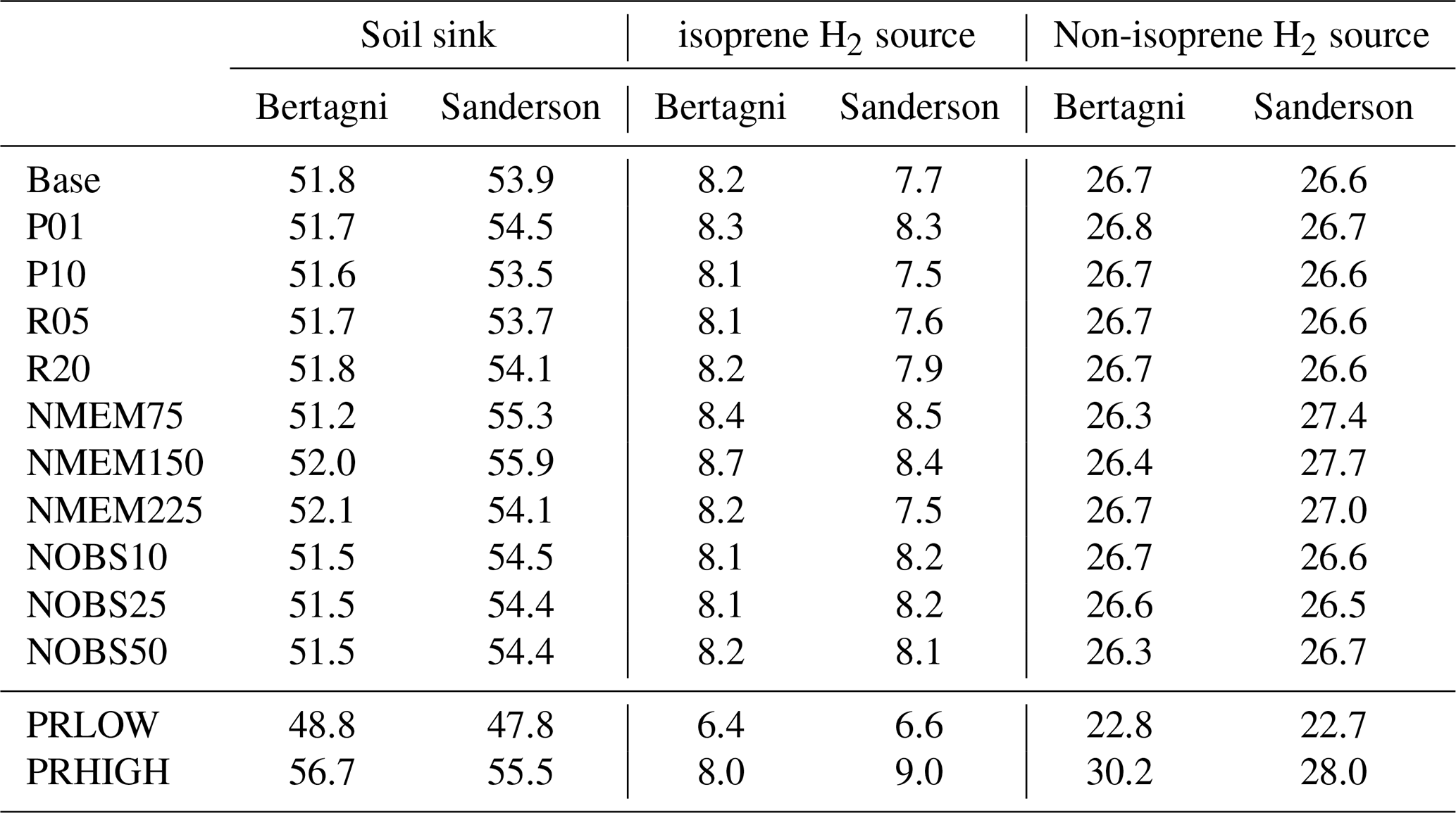
As shown in the previous sections, the choice of inversion parameters strongly influences the posterior fluxes inferred by the inversion. To quantify this impact, we systematically vary the number of ensemble members, observation subsets, scaling factors for the observation error variance (R), and scaling factors for the uncertainty assigned to each statevector element in space and time (P). This approach also provides a practical estimate of uncertainty within our ensemble Kalman filter-based inversion framework, for which formal posterior error estimates are otherwise not available. We perform the analysis using the best-performing configurations for the Sanderson and Bertagni schemes identified in Fig. 3.1, as well as alternative configurations shown in the same figure to assess sensitivity to the absolute magnitude of the priors. These alternative configurations correspond to prior source–sink pairs (photochemical source, soil sink) of (33.1, 40.3) and (44.1, 51.8) Tg yr−1 for the Sanderson experiments, and (33.1, 40.4) and (44.1, 67.3) Tg yr−1 for the Bertagni experiments. We note that scaling the prior flux magnitude also proportionally scales the assumed absolute uncertainty in flux space, thereby modifying both the prior statevector and its associated covariance matrix.
Table D1 shows that the posterior fluxes are most dependent on the absolute magnitude of the prior fluxes. In comparison, the posterior fluxes are relatively insensitive to the remaining inversion parameters. We find that the soil sink and the non-isoprene photochemical source are the most sta-ble flux components, whereas the isoprene H2 source shows larger variability, likely reflecting its spatial correlation with the soil sink. Apart from the absolute prior magnitudes, the largest deviations from the Base run occur in experiments with suboptimal configurations, i.e. when using a reduced number of ensemble members or a strongly limited observational network. This highlights the importance of sufficient ensemble size and observational coverage for robust flux optimisation. Even under these less constrained configurations, the inferred flux changes remain moderate, giving additional confidence to the robustness of our derived global H2 budget. Based on all experiments in Table D1, we derive a posterior error range of 47.8–56.7 Tg yr−1 for the soil sink and 29.2–38.2 Tg yr−1 for the photochemical source. For the individual photochemical source components, we derive an isoprene H2 source of 6.4–9.0 Tg yr−1, and a non-isoprene H2 source of 22.8–30.2 Tg yr−1.
Table D1Posterior H2 fluxes from 11 offline inversions (2003–2023) in which key inversion parameters were systematically perturbed. The final two rows show posterior H2 fluxes from two online inversions (2014–2023) using alternative source–sink configurations for the photochemical source and soil sink. All fluxes are in Tg yr−1. Experiment definitions: Base denotes the “best-performing” inversions used to derive our main results; P01/P10 denote scaling factors for the prior statevector uncertainty P (0.1×, 1.0×); R05/R20 denote scaling factors for the observational error variance R (0.5×, 2.0×); NMEM75/150/225 denote the number of ensemble members; NOBS10/25/50 denote reduced observation subsets (10 %, 25 %, 50 %); PRLOW/PRHIGH denote alternative (lower or higher) prior magnitudes.
We find that both inversions show a strongly negative global correlation between the posterior soil sink and isoprene H2 source fluxes (Fig. E1). This shows that regions with stronger soil uptake (more negative flux values) tend to coincide with regions of higher isoprene H2 emissions (more positive flux values), reflecting spatial co-location of strong flux magnitudes with opposite sign conventions, particularly in the tropics. Both inversions also show a negative correlation between the soil sink and the non-isoprene H2 source. This similarly reflects that regions of enhanced soil uptake tend to coincide with regions of enhanced emissions from this source category, despite limited spatial overlap in their dominant source regions. In contrast, the two H2 source terms (isoprene and non-isoprene) show a positive correlation, indicating that regions with stronger emissions in one source category tend to also exhibit stronger emissions in the other. This suggests a shared spatial structure in the distribution of H2 sources across regions.
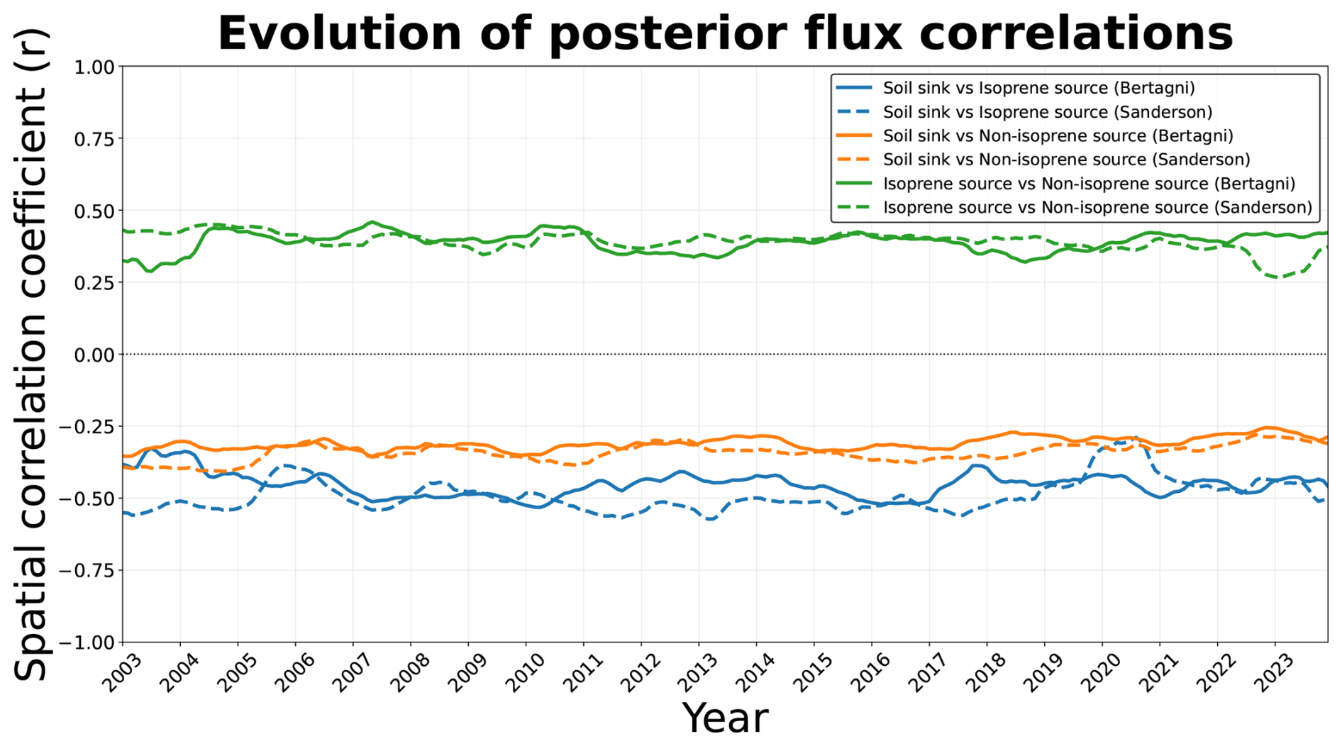
Figure E1Temporal evolution of area-weighted spatial correlations between posterior ensemble-mean H2 flux field. Each panel shows the Pearson correlation computed across grid cells for a given month, using cosine-latitude weighting to account for grid-cell area. Correlations are calculated from posterior ensemble-mean flux fields rather than individual ensemble members, because the ensemble Kalman filter inversion substantially reduces posterior spread, leaving residual ensemble-member variability at the grid scale comparatively small.
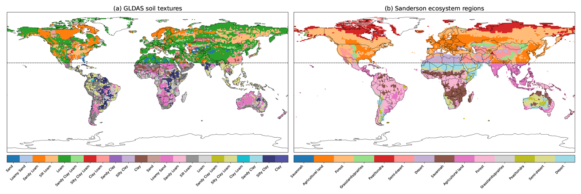
Figure F1Regions used in the soil sink schemes and inversions (statevector regions). The left panel shows the 22 GLDAS soil texture classes, while the right panel shows the 14 Sanderson ecosystem regions. Both are split at 25° N to approximately balance the land area between the Northern and Southern portion of the domain (dotted black line).
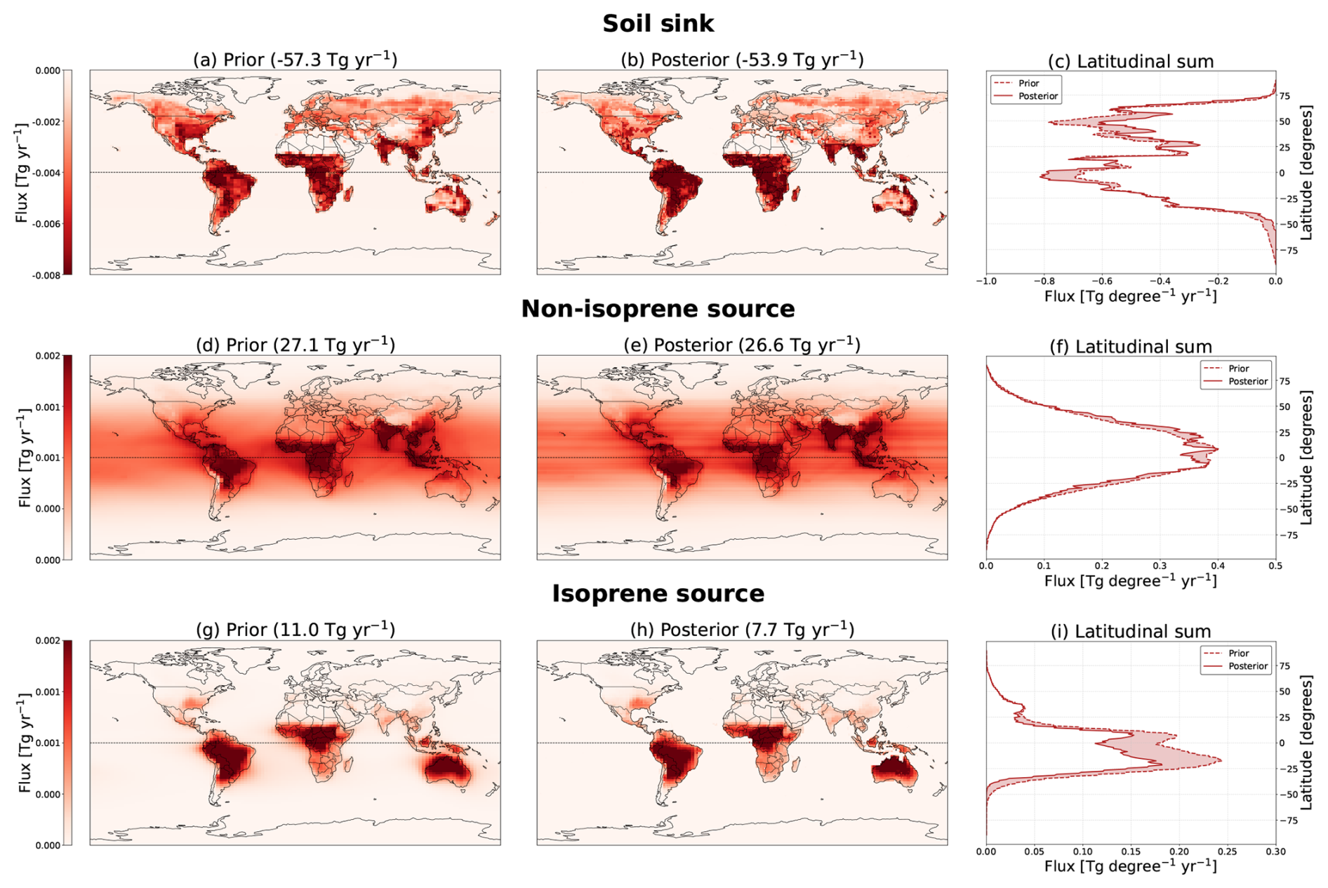
Figure F2Annual mean fluxes (2003–2023) for the Sanderson inversion, with corresponding latitudinal distributions.
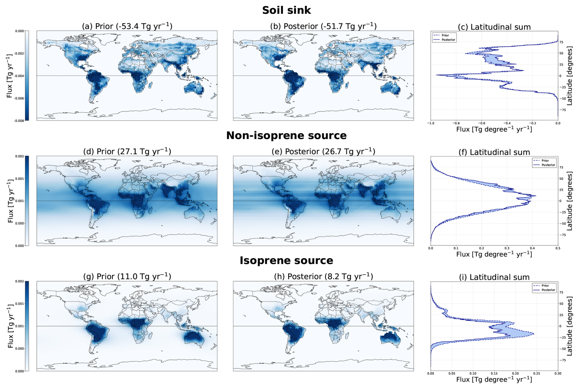
Figure F3Annual mean fluxes (2003–2023) for the Bertagni inversion, with corresponding latitudinal distributions.
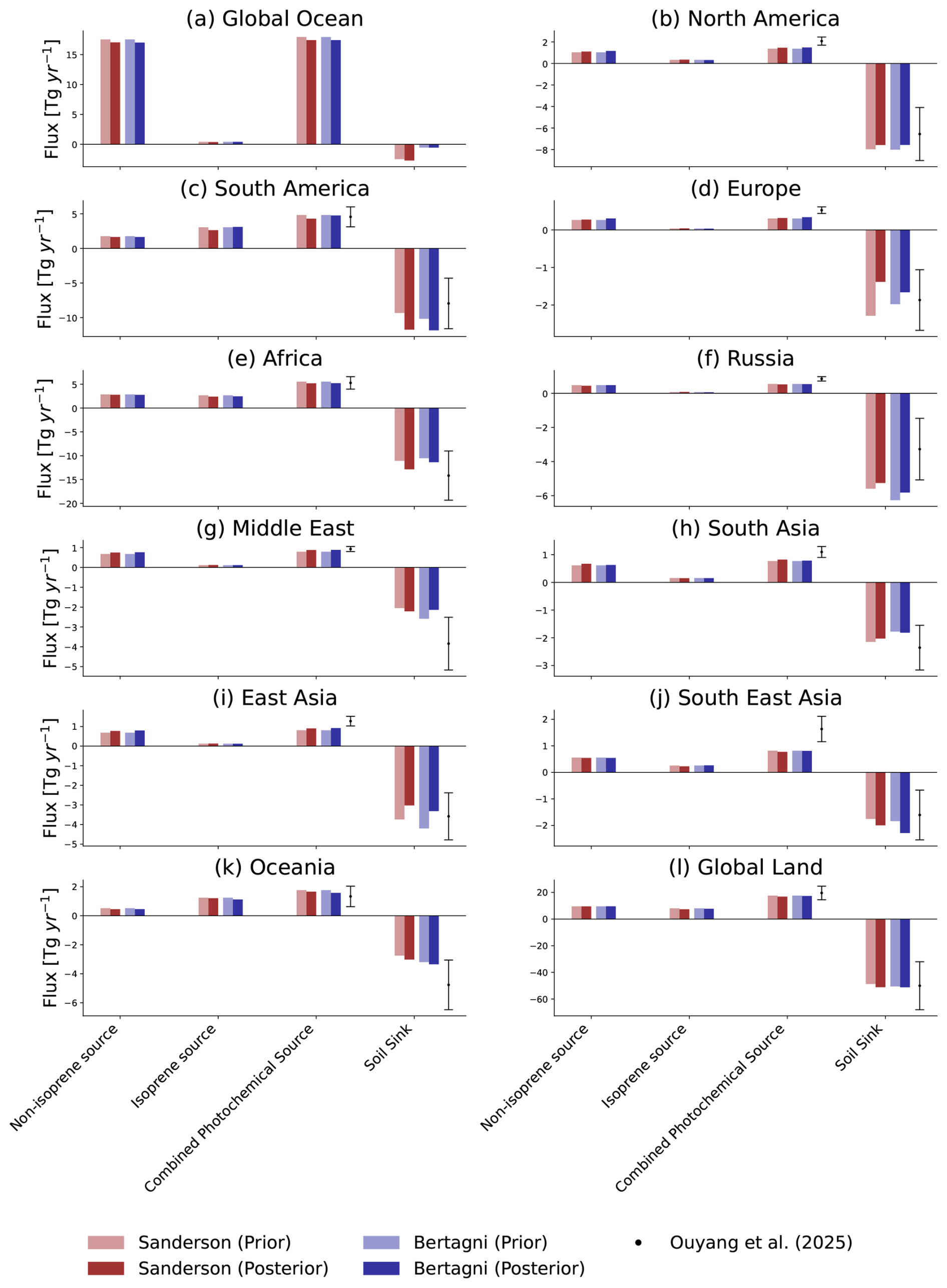
Figure F4Fluxes per RECCAP2 region (2003–2023 mean), ordered from left to right as: Sanderson prior, Sanderson posterior, Bertagni prior, and Bertagni posterior. Black dots with whiskers show the ensemble mean and one standard deviation range from Ouyang et al. (2025). A small soil sink occurs over global ocean regions in our results (Sanderson: 2.7 Tg yr−1; Bertagni: 0.6 Tg yr−1), as some islands are included in the RECCAP2 ocean regions.
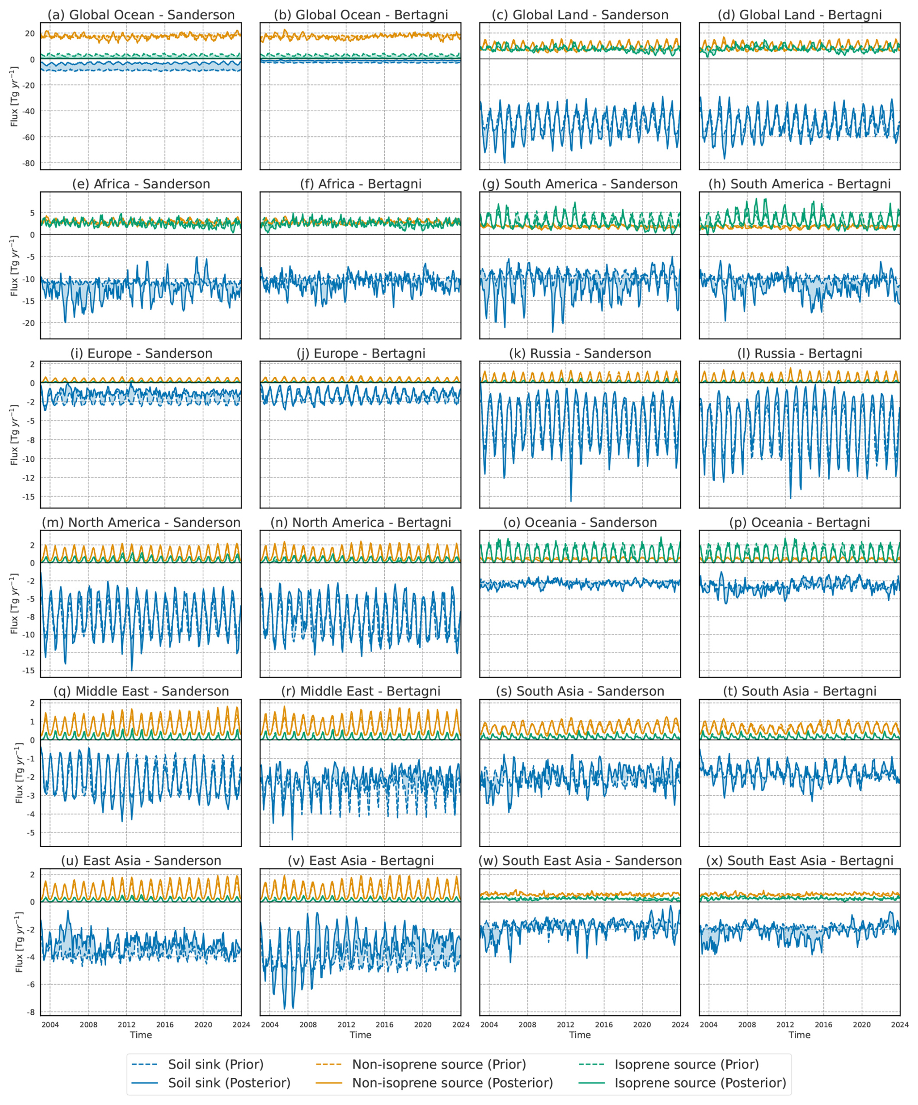
Figure F5Monthly simulated fluxes for each RECCAP2 region in the Sanderson and Bertagni inversions. Prior fluxes are shown as dotted lines and posterior fluxes as solid lines. A small soil sink occurs over global ocean regions in our results (Sanderson: 2.7 Tg yr−1; Bertagni: 0.6 Tg yr−1), as some islands are included in the RECCAP2 ocean regions.
Table F1Overview of measurement networks used in this study, filtered for our study period (2003–2023). Sampling interval denotes the modal (i.e. most frequently occurring) time between consecutive measurements, computed across all stations or flight tracks within each network.
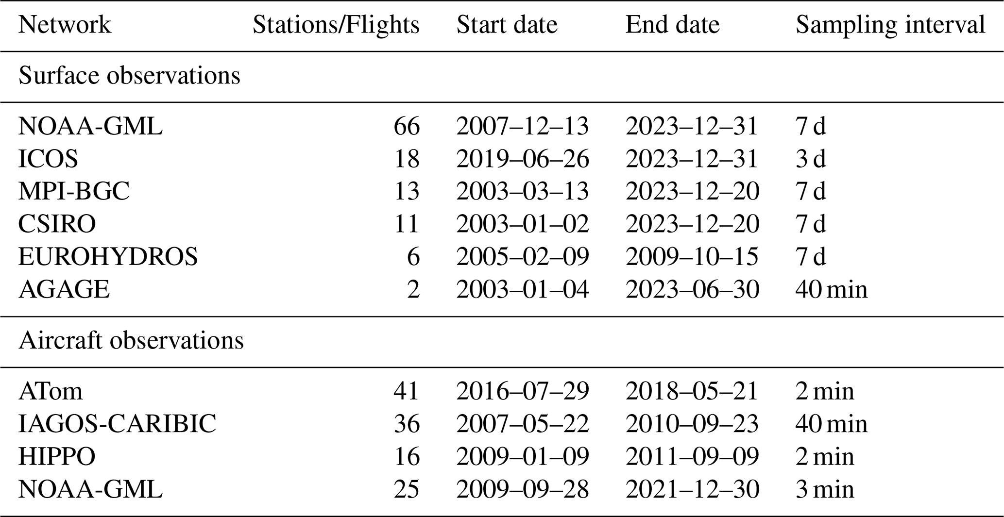
Table F2Evaluation of posterior H2 mole fractions against independent aircraft data. Shown are the mean posterior MAE [ppb] binned by altitude and latitude for the Sanderson (left) and Bertagni (right) inversions for each measurement campaign.
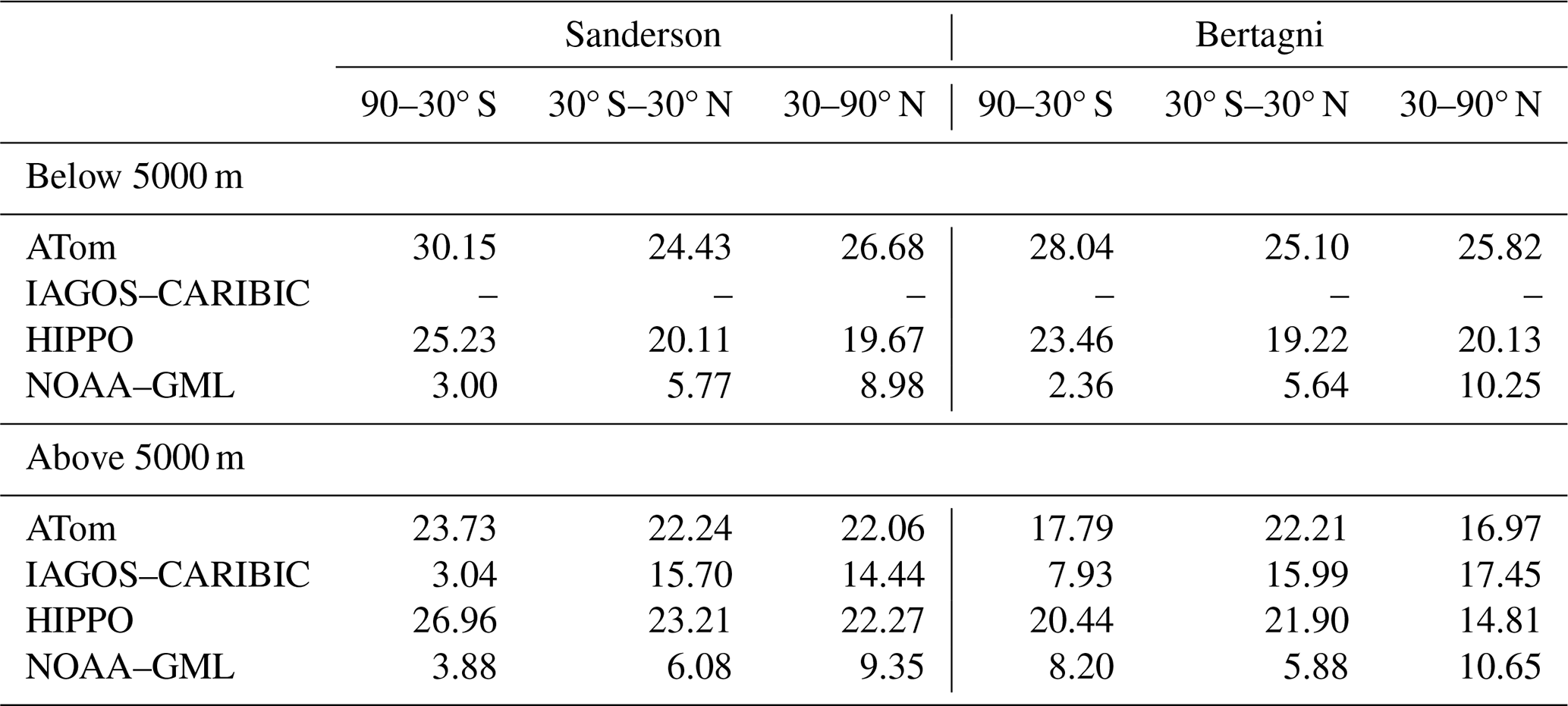
Table F3Seasonality of the monthly H2 soil sink across RECCAP2 regions. Values show the mean annual seasonal range in Tg yr−1 followed by the mean month of maximum uptake calculated over the 2003–2023 region.
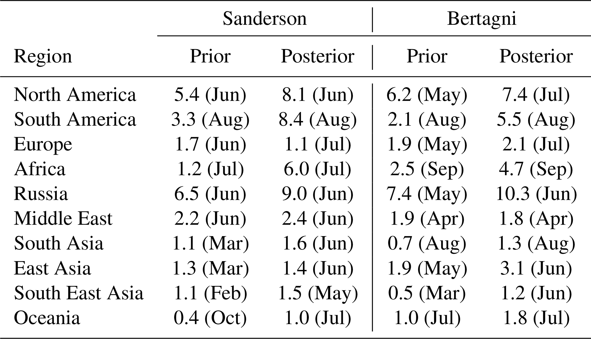
Table F4Correlation statistics between monthly posterior soil sink anomalies and the Oceanic Niño Index (ONI; units °C). Monthly soil sink anomalies are computed as deviations from a month-specific climatology over the final 10 years of the inversions (2014–2024). Metric r is the Pearson correlation coefficient, and p the p-value. Only regions where p<0.05 in either the Sanderson or Bertagni inversion are shown.
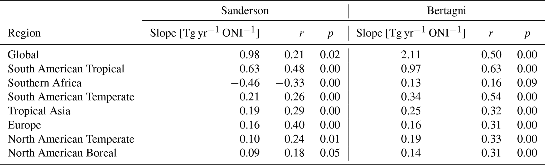
The CarbonTracker and TM5-MP living codebases are openly available via https://git.wur.nl/ctdas (last access: 28 May 2026) and https://ci.tno.nl/gitlab/tm5/tm5-mp (last access: 28 May 2026), respectively. The two-dimensional prior and posterior monthly H2 fluxes produced in this study are archived on https://doi.org/10.5281/zenodo.20427212 (Stroo, 2026) at 1 × 1 resolution. Daily three-dimensional flux fields are available upon request.
FS performed the simulations, analysed and synthesised the data, produced the figures, and led the writing of the manuscript. WP supervised the study and contributed to the conceptualisation and design of the project, manuscript structure, and writing. JH contributed to the development of the model code and the design of the simulations. MK contributed to the conceptualisation and design of the project. WP, JH, and MK reviewed the manuscript.
The contact author has declared that none of the authors has any competing interests.
Publisher's note: Copernicus Publications remains neutral with regard to jurisdictional claims made in the text, published maps, institutional affiliations, or any other geographical representation in this paper. The authors bear the ultimate responsibility for providing appropriate place names. Views expressed in the text are those of the authors and do not necessarily reflect the views of the publisher.
We contacted the PIs of all observational datasets used in this study and gratefully acknowledge the EUROHYDROS (Batenburg et al., 2011), NOAA-GML (Pétron et al., 2024), CSIRO-GASLAB (Krummel et al., 2025), MPI-BGC (Jordan et al., 2024), and ICOS (Apadula et al., 2025) networks for surface flask H2 observations, as well as the AGAGE network (Prinn et al., 2025) for in situ H2 observations. We also acknowledge the HIPPO (Wofsy, 2011; Wofsy et al., 2017), ATom (Montzka et al., 2019; Thompson et al., 2022; Wofsy et al., 2021), NOAA-GML (McKain et al., 2022; Sweeney et al., 2015), and IAGOS-CARIBIC (Batenburg et al., 2016) campaigns for aircraft H2 observations. ATom additionally provided CH2O and photolysis rate constant (JaCH2O) aircraft observations (Hall et al., 2018; Hanisco et al., 2019; Wofsy et al., 2021). AI tools (ChatGPT and GitHub Copilot) were used to assist with language editing, manuscript readability, brainstorming, and coding support for analysis scripts. No generative AI tools were used to generate scientific interpretations or conclusions. All outputs were reviewed and validated by the contact author.
This research has been supported by the Nationaal Programma Groningen and the European Union via the subsidy “Waterstof Werkt: Train and Learn Hub” and by the Gas & Hydrogen Partnerships Shell Nederland. All simulations were performed on the HPC cluster Aether at the University of Bremen, financed by DFG within the scope of the Excellence Initiative.
This paper was edited by Gunnar Myhre and reviewed by Alexander Tardito Chaudhri and one anonymous referee.
Apadula, F., Arnold, S., Bergamaschi, P., Biermann, T., Chen, H., Colomb, A., Conil, S., Couret, C., Cristofanelli, P., De Mazière, M., Delmotte, M., Di Iorio, T., Emmenegger, L., Forster, G., Frumau, A., Harris, E., Haszpra, L., Hatakka, J., Heliasz, M., Heltai, D., Hensen, A., Hermansen, O., Hoheisel, A., Kneuer, T., Komínková, K., Kubistin, D., Larmanou, E., Laurent, O., Laurila, T., Lehner, I., Lehtinen, K., Leskinen, A., Leuenberger, M., Levula, J., Lindauer, M., Lopez, M., Lund Myhre, C., Lunder, C., Mammarella, I., Manca, G., Manning, A., Marek, M. V., Marklund, P., Meinhardt, F., Miettinen, P., Molnár, M., Montaguti, S., Mölder, M., Müller-Williams, J., O'Doherty, S., Ottosson-Löfvenius, M., Piacentino, S., Pichon, J.-M., Pitt, J., Platt, S. M., Plaß-Dülmer, C., Ramonet, M., Rivas-Soriano, P., Roulet, Y.-A., Scheeren, B., Schmidt, M., Schumacher, M., Sferlazzo, D., Sha, M. K., Smith, P., Stanley, K., Steinbacher, M., Sørensen, L. L., Trisolino, P., Vítková, G., Ylisirniö, A., Yver-Kwok, C., Zazzeri, G., Zwerschke, E., di Sarra, A., ICOS ATC-Laboratoires des Sciences du Climat et de L'Environnement (LSCE), France, ICOS Central Radiocarbon Laboratory (CRL), Germany, ICOS Flask And Calibration Laboratory (FCL), Germany, ICOS-CAL-CRL, and ICOS-CAL-FCL: ICOS Atmosphere Release 2025-1 of Level 2 Greenhouse Gas Mole Fractions of CO2, CH4, N2O, CO, meteorology and 14CO2, and flask samples analysed for CO2, CH4, N2O, CO, H2, SF6, delta 13C CO2, delta18OCO2, delta O2N2 and 14C, ICOS ATC time series,ICOS ATC Flask time series Version Number: 1.0, https://doi.org/10.18160/PP29-9CNZ, 2025. a, b
Aronson, E. L., Dierick, D., Botthoff, J. K., Oberbauer, S., Zelikova, T. J., Harmon, T. C., Rundel, P., Johnson, R. F., Swanson, A. C., Pinto‐Tomás, A. A., Artavia-León, A., Matarrita-Carranza, B., and Allen, M. F.: ENSO-Influenced Drought Drives Methane Flux Dynamics in a Tropical Wet Forest Soil, J. Geophys. Res.-Biogeo., 124, 2267–2276, https://doi.org/10.1029/2018JG004832, 2019. a
Barnston, A. G., Chelliah, M., and Goldenberg, S. B.: Documentation of a highly ENSO-related sst region in the equatorial pacific: Research note, Atmosphere-Ocean, 35, 367–383, https://doi.org/10.1080/07055900.1997.9649597, 1997. a
Batenburg, A., Schuck, T., Baker, A., Zahn, A., Brenninkmeijer, C., and Roeckmann, T.: H2 mixing ratio and isotope data from CARIBIC project, figshare, https://doi.org/10.6084/M9.FIGSHARE.2068992.V1, 2016. a, b
Batenburg, A. M., Walter, S., Pieterse, G., Levin, I., Schmidt, M., Jordan, A., Hammer, S., Yver, C., and Röckmann, T.: Temporal and spatial variability of the stable isotopic composition of atmospheric molecular hydrogen: observations at six EUROHYDROS stations, Atmos. Chem. Phys., 11, 6985–6999, https://doi.org/10.5194/acp-11-6985-2011, 2011. a, b
Bertagni, M. B., Paulot, F., and Porporato, A.: Moisture Fluctuations Modulate Abiotic and Biotic Limitations of H2 Soil Uptake, Global Biogeochem. Cy., 35, https://doi.org/10.1029/2021GB006987, 2021. a, b
Bousquet, P., Yver, C., Pison, I., Li, Y. S., Fortems, A., Hauglustaine, D., Szopa, S., Rayner, P. J., Novelli, P., Langenfelds, R., Steele, P., Ramonet, M., Schmidt, M., Foster, P., Morfopoulos, C., and Ciais, P.: A three-dimensional synthesis inversion of the molecular hydrogen cycle: Sources and sinks budget and implications for the soil uptake, J. Geophys. Res., 116, D01302, https://doi.org/10.1029/2010JD014599, 2011. a, b, c, d, e
Chen, Q., Popa, M. E., Batenburg, A. M., and Röckmann, T.: Isotopic signatures of production and uptake of H2 by soil, Atmos. Chem. Phys., 15, 13003–13021, https://doi.org/10.5194/acp-15-13003-2015, 2015. a
Ciais, P., Bastos, A., Chevallier, F., Lauerwald, R., Poulter, B., Canadell, J. G., Hugelius, G., Jackson, R. B., Jain, A., Jones, M., Kondo, M., Luijkx, I. T., Patra, P. K., Peters, W., Pongratz, J., Petrescu, A. M. R., Piao, S., Qiu, C., Von Randow, C., Regnier, P., Saunois, M., Scholes, R., Shvidenko, A., Tian, H., Yang, H., Wang, X., and Zheng, B.: Definitions and methods to estimate regional land carbon fluxes for the second phase of the REgional Carbon Cycle Assessment and Processes Project (RECCAP-2), Geosci. Model Dev., 15, 1289–1316, https://doi.org/10.5194/gmd-15-1289-2022, 2022. a
Conrad, R.: Soil microorganisms as controllers of atmospheric trace gases (H2, CO, CH4, OCS, N2O, and NO), Microbiol. Rev., 60, 609–640, https://doi.org/10.1128/mr.60.4.609-640.1996, 1996. a
Conrad, R., Mayer, H.-P., and Wüst, M.: Temporal change of gas metabolism by hydrogen-syntrophic methanogenic bacterial associations in anoxic paddy soil, FEMS Microbiol. Lett., 62, 265–273, https://doi.org/10.1111/j.1574-6968.1989.tb03701.x, 1989. a
Conte, L., Szopa, S., Séférian, R., and Bopp, L.: The oceanic cycle of carbon monoxide and its emissions to the atmosphere, Biogeosciences, 16, 881–902, https://doi.org/10.5194/bg-16-881-2019, 2019. a
Cowan, N., Roberts, T., Hanlon, M., Bezanger, A., Toteva, G., Tweedie, A., Yeung, K., Deshpande, A., Levy, P., Skiba, U., Nemitz, E., and Drewer, J.: Quantifying the soil sink of atmospheric hydrogen: a full year of field measurements from grassland and forest soils in the UK, Biogeosciences, 22, 3449–3461, https://doi.org/10.5194/bg-22-3449-2025, 2025. a
De Kleijne, K., Huijbregts, M. A. J., Knobloch, F., Van Zelm, R., Hilbers, J. P., De Coninck, H., and Hanssen, S. V.: Worldwide greenhouse gas emissions of green hydrogen production and transport, Nature Energy, https://doi.org/10.1038/s41560-024-01563-1, 2024. a
Ehhalt, D. H. and Rohrer, F.: The tropospheric cycle of H2: a critical review, Tellus B, 61, 500–535, https://doi.org/10.1111/j.1600-0889.2009.00416.x, 2009. a, b
Ehhalt, D. H. and Rohrer, F.: The dependence of soil H2 uptake on temperature and moisture: a reanalysis of laboratory data, Tellus B, 63, 1040, https://doi.org/10.1111/j.1600-0889.2011.00581.x, 2011. a
Feng, L., Smith, S. J., Braun, C., Crippa, M., Gidden, M. J., Hoesly, R., Klimont, Z., van Marle, M., van den Berg, M., and van der Werf, G. R.: The generation of gridded emissions data for CMIP6, Geosci. Model Dev., 13, 461–482, https://doi.org/10.5194/gmd-13-461-2020, 2020. a
Gibson, J., Eby, P., and Jaggi, A.: Natural isotope fingerprinting of produced hydrogen and its potential applications to the hydrogen economy, Int. J. Hydrogen Energ., 66, 468–478, https://doi.org/10.1016/j.ijhydene.2024.04.077, 2024. a
Gros, V., Peeken, I., Bluhm, K., Zöllner, E., Sarda-Esteve, R., and Bonsang, B.: Carbon monoxide emissions by phytoplankton: evidence from laboratory experiments, Environ. Chem., 6, 369, https://doi.org/10.1071/EN09020, 2009. a
Guenther, A. B., Jiang, X., Heald, C. L., Sakulyanontvittaya, T., Duhl, T., Emmons, L. K., and Wang, X.: The Model of Emissions of Gases and Aerosols from Nature version 2.1 (MEGAN2.1): an extended and updated framework for modeling biogenic emissions, Geosci. Model Dev., 5, 1471–1492, https://doi.org/10.5194/gmd-5-1471-2012, 2012. a
Hall, S. R., Ullmann, K., Prather, M. J., Flynn, C. M., Murray, L. T., Fiore, A. M., Correa, G., Strode, S. A., Steenrod, S. D., Lamarque, J.-F., Guth, J., Josse, B., Flemming, J., Huijnen, V., Abraham, N. L., and Archibald, A. T.: Cloud impacts on photochemistry: building a climatology of photolysis rates from the Atmospheric Tomography mission, Atmos. Chem. Phys., 18, 16809–16828, https://doi.org/10.5194/acp-18-16809-2018, 2018. a, b
Hanisco, T., Hannun, R., St.Clair, J., and Wolfe, G.: Atmospheric Tomography Mission (ATom)ATom: L2 Measurements of In Situ Airborne Formaldehyde (ISAF), ORNL Distributed Active Archive Center, https://doi.org/10.3334/ORNLDAAC/1730, 2019. a, b
Hauglustaine, D. A. and Ehhalt, D. H.: A three-dimensional model of molecular hydrogen in the troposphere: TROPOSPHERIC MOLECULAR HYDROGEN, J. Geophys. Res.-Atmos., 107, ACH 4-1–ACH 4-16, https://doi.org/10.1029/2001JD001156, 2002. a
Hersbach, H., Bell, B., Berrisford, P., Hirahara, S., Horányi, A., Muñoz-Sabater, J., Nicolas, J., Peubey, C., Radu, R., Schepers, D., Simmons, A., Soci, C., Abdalla, S., Abellan, X., Balsamo, G., Bechtold, P., Biavati, G., Bidlot, J., Bonavita, M., De Chiara, G., Dahlgren, P., Dee, D., Diamantakis, M., Dragani, R., Flemming, J., Forbes, R., Fuentes, M., Geer, A., Haimberger, L., Healy, S., Hogan, R. J., Hólm, E., Janisková, M., Keeley, S., Laloyaux, P., Lopez, P., Lupu, C., Radnoti, G., De Rosnay, P., Rozum, I., Vamborg, F., Villaume, S., and Thépaut, J.: The ERA5 global reanalysis, Q. J. Roy. Meteor. Soc., 146, 1999–2049, https://doi.org/10.1002/qj.3803, 2020. a, b
Hoesly, R. M., Smith, S. J., Feng, L., Klimont, Z., Janssens-Maenhout, G., Pitkanen, T., Seibert, J. J., Vu, L., Andres, R. J., Bolt, R. M., Bond, T. C., Dawidowski, L., Kholod, N., Kurokawa, J.-I., Li, M., Liu, L., Lu, Z., Moura, M. C. P., O'Rourke, P. R., and Zhang, Q.: Historical (1750–2014) anthropogenic emissions of reactive gases and aerosols from the Community Emissions Data System (CEDS), Geosci. Model Dev., 11, 369–408, https://doi.org/10.5194/gmd-11-369-2018, 2018. a
IEA: The Future of Hydrogen, Tech. rep., International Energy Agency, https://www.iea.org/reports/the-future-of-hydrogen (last access: 28 May 2026), 2019. a, b
IEA: Global Hydrogen Review 2023, Tech. rep., International Energy Agency, https://www.iea.org/reports/global-hydrogen-review-2023 (last access: 28 May 2026), 2023. a, b
Inness, A., Ades, M., Agustí-Panareda, A., Barré, J., Benedictow, A., Blechschmidt, A.-M., Dominguez, J. J., Engelen, R., Eskes, H., Flemming, J., Huijnen, V., Jones, L., Kipling, Z., Massart, S., Parrington, M., Peuch, V.-H., Razinger, M., Remy, S., Schulz, M., and Suttie, M.: The CAMS reanalysis of atmospheric composition, Atmos. Chem. Phys., 19, 3515–3556, https://doi.org/10.5194/acp-19-3515-2019, 2019. a, b
Jordan, A. and Steinberg, B.: Calibration of atmospheric hydrogen measurements, Atmos. Meas. Tech., 4, 509–521, https://doi.org/10.5194/amt-4-509-2011, 2011. a
Jordan, A., Moossen, H., Rothe, M., Brand, W., Heimann, M., Zaehle, S., and Rödenbeck, C.: Atmospheric flask sampling program of MPI-BGC, version 2024.1, Edmond, https://doi.org/10.17617/3.S3KHMS, 2024. a, b
Krol, M., Houweling, S., Bregman, B., van den Broek, M., Segers, A., van Velthoven, P., Peters, W., Dentener, F., and Bergamaschi, P.: The two-way nested global chemistry-transport zoom model TM5: algorithm and applications, Atmos. Chem. Phys., 5, 417–432, https://doi.org/10.5194/acp-5-417-2005, 2005. a
Krummel, P., Langenfelds, R., Guerette, E., and Loh, Z.: Atmospheric H2 at sites from the Commonwealth Scientific and Industrial Research Organisation (CSIRO) global monitoring network, World Data Centre for Greenhouse Gases, https://doi.org/10.50849/WDCGG_H2_ALL_2025, 2025. a, b
McCarthy, M. C.: The hydrogen isotopic composition of water vapor entering the stratosphere inferred from high-precision measurements of CHD3 and HD, J. Geophys. Res., 109, D07304, https://doi.org/10.1029/2003JD004003, 2004. a
McKain, K., Sweeney, C., Crotwell, A., Crotwell, M., Higgs, J., Legard, T., Madronich, M., Miller, J., Moglia, E., Mund, J., Neff, D., Wolter, S., and NOAA Global Monitoring Laboratory: NOAA Global Greenhouse Gas Reference Network Flask-Air PFP Sample Measurements of CO2, CH4, CO, N2O, H2, SF6 and isotopic ratios collected from aircraft vertical profiles, NOAA Global Monitoring Laboratory, https://doi.org/10.15138/39HR-9N34, 2022. a, b
Montzka, S., Moore, F., and Sweeney, C.: Atmospheric Tomography Mission (ATom)ATom: L2 Measurements from the Programmable Flask Package (PFP) Whole Air Sampler, ORNL Distributed Active Archive Center, https://doi.org/10.3334/ORNLDAAC/1746, 2019. a, b
Naik, V., Voulgarakis, A., Fiore, A. M., Horowitz, L. W., Lamarque, J.-F., Lin, M., Prather, M. J., Young, P. J., Bergmann, D., Cameron-Smith, P. J., Cionni, I., Collins, W. J., Dalsøren, S. B., Doherty, R., Eyring, V., Faluvegi, G., Folberth, G. A., Josse, B., Lee, Y. H., MacKenzie, I. A., Nagashima, T., van Noije, T. P. C., Plummer, D. A., Righi, M., Rumbold, S. T., Skeie, R., Shindell, D. T., Stevenson, D. S., Strode, S., Sudo, K., Szopa, S., and Zeng, G.: Preindustrial to present-day changes in tropospheric hydroxyl radical and methane lifetime from the Atmospheric Chemistry and Climate Model Intercomparison Project (ACCMIP), Atmos. Chem. Phys., 13, 5277–5298, https://doi.org/10.5194/acp-13-5277-2013, 2013. a
Naus, S., Montzka, S. A., Patra, P. K., and Krol, M. C.: A three-dimensional-model inversion of methyl chloroform to constrain the atmospheric oxidative capacity, Atmos. Chem. Phys., 21, 4809–4824, https://doi.org/10.5194/acp-21-4809-2021, 2021. a
NOAA Global Monitoring Laboratory: Curve Fitting Methods Applied to Time Series (CCGCRV), https://gml.noaa.gov/ccgg/mbl/crvfit/ (last access: 28 May 2026), 2026. a, b, c
Novelli, P., Lang, P., Masarie, K., Hurst, D., Myers, R., and Elkins, J.: Molecular hydrogen in the troposphere: Global distribution and budget, J. Geophys. Res., 104, 30427–30444, https://doi.org/10.1029/1999JD900788, 1999. a
Ocko, I. B. and Hamburg, S. P.: Climate consequences of hydrogen emissions, Atmos. Chem. Phys., 22, 9349–9368, https://doi.org/10.5194/acp-22-9349-2022, 2022. a
Ouyang, Z., Jackson, R. B., Saunois, M., Canadell, J. G., Zhao, Y., Morfopoulos, C., Krummel, P. B., Patra, P. K., Peters, G. P., Dennison, F., Gasser, T., Archibald, A. T., Arora, V., Baudoin, G., Chandra, N., Ciais, P., Davis, S. J., Feron, S., Guo, F., Hauglustaine, D., Jones, C. D., Jones, M. W., Kato, E., Kennedy, D., Knauer, J., Lienert, S., Lombardozzi, D., Melton, J. R., Nabel, J. E., O'Sullivan, M., Pétron, G., Poulter, B., Rogelj, J., Sandoval Calle, D., Smith, P., Suntharalingam, P., Tian, H., Wang, C., and Wiltshire, A.: The global hydrogen budget, Nature, 648, 616–624, https://doi.org/10.1038/s41586-025-09806-1, 2025. a, b, c, d, e, f, g, h, i, j, k, l, m, n, o, p, q
Patra, P. K., Krol, M. C., Prinn, R. G., Takigawa, M., Mühle, J., Montzka, S. A., Lal, S., Yamashita, Y., Naus, S., Chandra, N., Weiss, R. F., Krummel, P. B., Fraser, P. J., O'Doherty, S., and Elkins, J. W.: Methyl Chloroform Continues to Constrain the Hydroxyl (OH) Variability in the Troposphere, J. Geophys. Res.-Atmos., 126, e2020JD033862, https://doi.org/10.1029/2020JD033862, 2021. a
Paulot, F., Paynter, D., Naik, V., Malyshev, S., Menzel, R., and Horowitz, L. W.: Global modeling of hydrogen using GFDL-AM4.1: Sensitivity of soil removal and radiative forcing, Int. J. Hydrogen Energ., 46, 13446–13460, https://doi.org/10.1016/j.ijhydene.2021.01.088, 2021. a
Percival, C. J. and Sander, S. P.: Chemical Kinetics and Photochemical Data for Use in Atmospheric Studies Evaluation Number 20, Tech. rep., Jet Propulsion Laboratory, California Institute of Technology, https://doi.org/10.48577/JPL.KFQ0TZ, 2026. a
Pieterse, G.: Modelling the global tropospheric molecular hydrogen cycle, Ph.D. thesis, Utrecht University, ISBN 978-94-6191-559-7, 2013. a
Pieterse, G., Krol, M. C., Batenburg, A. M., Steele, L. P., Krummel, P. B., Langenfelds, R. L., and Röckmann, T.: Global modelling of H2 mixing ratios and isotopic compositions with the TM5 model, Atmos. Chem. Phys., 11, 7001–7026, https://doi.org/10.5194/acp-11-7001-2011, 2011. a, b, c
Pieterse, G., Krol, M., Batenburg, A., Brenninkmeijer, C., Popa, E., O'Doherty, S., Grant, A., Steele, L., Krummel, P., Langenfelds, R., Wang, H., Vermeulen, A., Schmidt, M., Yver, C., Jordan, A., Engel, A., Fisher, R., Lowry, D., Nisbet, E., and Röckmann, T.: Reassessing the variability in atmospheric H2 using the two-way nested TM5 model, J. Geophys. Res., https://doi.org/10.1002/jgrd.50204, 2013. a, b, c, d, e, f
Pison, I., Bousquet, P., Chevallier, F., Szopa, S., and Hauglustaine, D.: Multi-species inversion of CH4, CO and H2 emissions from surface measurements, Atmos. Chem. Phys., 9, 5281–5297, https://doi.org/10.5194/acp-9-5281-2009, 2009. a, b, c, d, e, f
Prather, M. J., Holmes, C. D., and Hsu, J.: Reactive greenhouse gas scenarios: Systematic exploration of uncertainties and the role of atmospheric chemistry, Geophys. Res. Lett., 39, 2012GL051440, https://doi.org/10.1029/2012GL051440, 2012. a
Price, H., Jaeglé, L., Rice, A., Quay, P., Novelli, P. C., and Gammon, R.: Global budget of molecular hydrogen and its deuterium content: Constraints from ground station, cruise, and aircraft observations, J. Geophys. Res., 112, D22108, https://doi.org/10.1029/2006JD008152, 2007. a, b
Prinn, R., Weiss, R., Arduini, J., Choi, H., Engel, A., Fraser, P., Ganesan, A., Harth, C., Hermansen, O., Kim, J., Krummel, P., Loh, Z., Lunder, C., Maione, M., Manning, A., Mitrevski, B., Mühle, J., O'Doherty, S., Park, S., Pitt, J., Reimann, S., Rigby, M., Saito, T., Salameh, P., Schmidt, R., Simmonds, P., Stanley, K., Stavert, A., Steele, P., Vollmer, M., Wagenhäuser, T., Wang, H., Wenger, A., Western, L., Yao, B., Young, D., Zhou, L., and Zhu, L.: The dataset of in-situ measurements of chemically and radiatively important atmospheric gases from the Advanced Global Atmospheric Gas Experiment (AGAGE) and affiliated stations, NASA Langley Research Center (LaRC) Data Host Facility (DHF), https://doi.org/10.60718/75D7-QE84, 2025. a, b
Pétron, G., Crotwell, A. M., Mund, J., Crotwell, M., Mefford, T., Thoning, K., Hall, B., Kitzis, D., Madronich, M., Moglia, E., Neff, D., Wolter, S., Jordan, A., Krummel, P., Langenfelds, R., and Patterson, J.: Atmospheric H2 observations from the NOAA Cooperative Global Air Sampling Network, Atmos. Meas. Tech., 17, 4803–4823, https://doi.org/10.5194/amt-17-4803-2024, 2024. a, b, c
Rahn, T., Eiler, J. M., Boering, K. A., Wennberg, P. O., McCarthy, M. C., Tyler, S., Schauffler, S., Donnelly, S., and Atlas, E.: Extreme deuterium enrichment in stratospheric hydrogen and the global atmospheric budget of H2, Nature, 424, 918–921, https://doi.org/10.1038/nature01917, 2003. a
Rhee, T. S., Brenninkmeijer, C. A. M., and Röckmann, T.: The overwhelming role of soils in the global atmospheric hydrogen cycle, Atmos. Chem. Phys., 6, 1611–1625, https://doi.org/10.5194/acp-6-1611-2006, 2006. a, b, c, d
Rodell, M., Houser, P. R., Jambor, U., Gottschalck, J., Mitchell, K., Meng, C.-J., Arsenault, K., Cosgrove, B., Radakovich, J., Bosilovich, M., Entin, J. K., Walker, J. P., Lohmann, D., and Toll, D.: The Global Land Data Assimilation System, B. Am. Meteor. Soc., 85, 381–394, https://doi.org/10.1175/BAMS-85-3-381, 2004. a
Röckmann, T., Rhee, T. S., and Engel, A.: Heavy hydrogen in the stratosphere, Atmos. Chem. Phys., 3, 2015–2023, https://doi.org/10.5194/acp-3-2015-2003, 2003. a
Sand, M., Skeie, R. B., Sandstad, M., Krishnan, S., Myhre, G., Bryant, H., Derwent, R., Hauglustaine, D., Paulot, F., Prather, M., and Stevenson, D.: A multi-model assessment of the Global Warming Potential of hydrogen, Commun. Earth Environ., 4, 1–12, https://doi.org/10.1038/s43247-023-00857-8, 2023. a, b, c, d
Sand, M., Ocko, I. B., Sun, T., Skeie, R. B., Hauglustaine, D. A., Warwick, N. J., Stevenson, D. S., Paulot, F., Myhre, G., Archibald, A. T., Sandstad, M., Krishnan, S., and Prather, M.: Climate impacts of hydrogen emissions, Nat. Rev. Earth Environ., https://doi.org/10.1038/s43017-026-00792-0, 2026. a
Sander, S. P., Friedl, R. R., Ravishankara, A. R., Golden, D. M., Kolb, C. E., Kurylo, M. J., Molina, M. J., Moortgat, G. K., Keller-Rudek, H., Finlayson-Pitts, B. J., Wine, P. H., Huie, R. E., and Orkin, V. L.: Chemical Kinetics and Photochemical Data for Use in Atmospheric Studies: Evaluation No. 15, Tech. Rep. JPL Publication 06-2, Jet Propulsion Laboratory, California Institute of Technology, https://science.jpl.nasa.gov/documents/1493/JPL_15_AllInOne.pdf (last access: 28 May 2026), 2006. a
Sanderson, M. G., Collins, W. J., Derwent, R. G., and Johnson, C. E.: Simulation of Global Hydrogen Levels Using a Lagrangian Three-Dimensional Model, J. Atmos. Chem., 46, 15–28, https://doi.org/10.1023/A:1024824223232, 2003. a, b
Smith-Downey, N. V., Randerson, J. T., and Eiler, J. M.: Temperature and moisture dependence of soil H2 uptake measured in the laboratory, Geophys. Res. Lett., 33, 2006GL026749, https://doi.org/10.1029/2006GL026749, 2006. a
Soulie, A., Granier, C., Darras, S., Zilbermann, N., Doumbia, T., Guevara, M., Jalkanen, J.-P., Keita, S., Liousse, C., Crippa, M., Guizzardi, D., Hoesly, R., and Smith, S. J.: Global anthropogenic emissions (CAMS-GLOB-ANT) for the Copernicus Atmosphere Monitoring Service simulations of air quality forecasts and reanalyses, Earth Syst. Sci. Data, 16, 2261–2279, https://doi.org/10.5194/essd-16-2261-2024, 2024. a
Stone, K., Chen, C., Solomon, S., Western, L. M., Krummel, P. B., Pétron, G., Mühle, J., and O'Doherty, S.: Constraining the atmospheric hydrogen oxidation and soil sink seasonal cycles using HFC-152a, Atmos. Chem. Phys., 26, 10241–10253, https://doi.org/10.5194/acp-26-10241-2026, 2026. a, b, c, d, e, f, g, h, i, j, k, l
Stroo, F.: Posterior and Prior fluxes and model code for the 2003–2023 H2 inversions, Zenodo [data set], https://doi.org/10.5281/zenodo.20427212, 2026. a
Sweeney, C., Karion, A., Wolter, S., Newberger, T., Guenther, D., Higgs, J. A., Andrews, A. E., Lang, P. M., Neff, D., Dlugokencky, E., Miller, J. B., Montzka, S. A., Miller, B. R., Masarie, K. A., Biraud, S. C., Novelli, P. C., Crotwell, M., Crotwell, A. M., Thoning, K., and Tans, P. P.: Seasonal climatology of CO2 across North America from aircraft measurements in the NOAA/ESRL Global Greenhouse Gas Reference Network, J. Geophys. Res.-Atmos., 120, 5155–5190, https://doi.org/10.1002/2014JD022591, 2015. a, b
Tardito Chaudhri, A. K. and Stevenson, D. S.: Soil deposition of atmospheric hydrogen constrained using planetary-scale observations, Atmos. Chem. Phys., 25, 7369–7385, https://doi.org/10.5194/acp-25-7369-2025, 2025. a, b, c, d, e, f, g, h, i, j
Thompson, C. R., Wofsy, S. C., Prather, M. J., Newman, P. A., Hanisco, T. F., Ryerson, T. B., Fahey, D. W., Apel, E. C., Brock, C. A., Brune, W. H., Froyd, K., Katich, J. M., Nicely, J. M., Peischl, J., Ray, E., Veres, P. R., Wang, S., Allen, H. M., Asher, E., Bian, H., Blake, D., Bourgeois, I., Budney, J., Bui, T. P., Butler, A., Campuzano-Jost, P., Chang, C., Chin, M., Commane, R., Correa, G., Crounse, J. D., Daube, B., Dibb, J. E., DiGangi, J. P., Diskin, G. S., Dollner, M., Elkins, J. W., Fiore, A. M., Flynn, C. M., Guo, H., Hall, S. R., Hannun, R. A., Hills, A., Hintsa, E. J., Hodzic, A., Hornbrook, R. S., Huey, L. G., Jimenez, J. L., Keeling, R. F., Kim, M. J., Kupc, A., Lacey, F., Lait, L. R., Lamarque, J.-F., Liu, J., McKain, K., Meinardi, S., Miller, D. O., Montzka, S. A., Moore, F. L., Morgan, E. J., Murphy, D. M., Murray, L. T., Nault, B. A., Neuman, J. A., Nguyen, L., Gonzalez, Y., Rollins, A., Rosenlof, K., Sargent, M., Schill, G., Schwarz, J. P., Clair, J. M. S., Steenrod, S. D., Stephens, B. B., Strahan, S. E., Strode, S. A., Sweeney, C., Thames, A. B., Ullmann, K., Wagner, N., Weber, R., Weinzierl, B., Wennberg, P. O., Williamson, C. J., Wolfe, G. M., and Zeng, L.: The NASA Atmospheric Tomography (ATom) Mission: Imaging the Chemistry of the Global Atmosphere, B. Am. Meteor. Soc., 103, E761–E790, https://doi.org/10.1175/BAMS-D-20-0315.1, 2022. a, b
Thoning, K. W., Tans, P. P., and Komhyr, W. D.: Atmospheric carbon dioxide at Mauna Loa Observatory: 2. Analysis of the NOAA GMCC data, 1974–1985, J. Geophys. Res.-Atmos., 94, 8549–8565, https://doi.org/10.1029/JD094iD06p08549, 1989. a, b, c
Tolk, L. F., Dolman, A. J., Meesters, A. G. C. A., and Peters, W.: A comparison of different inverse carbon flux estimation approaches for application on a regional domain, Atmos. Chem. Phys., 11, 10349–10365, https://doi.org/10.5194/acp-11-10349-2011, 2011. a
Trapani, D., Marocco, P., Gandiglio, M., and Santarelli, M.: Hydrogen leakages across the supply chain: Current estimates and future scenarios, Int. J. Hydrogen Energ., 145, 1084–1095, https://doi.org/10.1016/j.ijhydene.2025.06.103, 2025. a
van der Laan-Luijkx, I. T., van der Velde, I. R., van der Veen, E., Tsuruta, A., Stanislawska, K., Babenhauserheide, A., Zhang, H. F., Liu, Y., He, W., Chen, H., Masarie, K. A., Krol, M. C., and Peters, W.: The CarbonTracker Data Assimilation Shell (CTDAS) v1.0: implementation and global carbon balance 2001–2015, Geosci. Model Dev., 10, 2785–2800, https://doi.org/10.5194/gmd-10-2785-2017, 2017. a, b
Van Der Werf, G. R., Randerson, J. T., Van Wees, D., Chen, Y., Giglio, L., Hall, J., Roland, V., Mu, M., Binte Shahid, S., Barsanti, K. C., Yokelson, R., and Morton, D. C.: Landscape fire emissions from the 5th version of the Global Fire Emissions Database (GFED5), Sci. Data, 12, 1870, https://doi.org/10.1038/s41597-025-06127-w, 2025. a
Vollmer, M. K., Walter, S., Bond, S. W., Soltic, P., and Röckmann, T.: Molecular hydrogen (H2) emissions and their isotopic signatures (H/D) from a motor vehicle: implications on atmospheric H2, Atmos. Chem. Phys., 10, 5707–5718, https://doi.org/10.5194/acp-10-5707-2010, 2010. a
Walter, S., Kock, A., Steinhoff, T., Fiedler, B., Fietzek, P., Kaiser, J., Krol, M., Popa, M. E., Chen, Q., Tanhua, T., and Röckmann, T.: Isotopic evidence for biogenic molecular hydrogen production in the Atlantic Ocean, Biogeosciences, 13, 323–340, https://doi.org/10.5194/bg-13-323-2016, 2016. a
Williams, J. and Van Noije, T.: On the upgrading of the modified Carbon Bond Mechanism IV for use in global Chemistry Transport Models, Scientific Report WR-08-02, KNMI, 2008. a
Williams, J. E., Boersma, K. F., Le Sager, P., and Verstraeten, W. W.: The high-resolution version of TM5-MP for optimized satellite retrievals: description and validation, Geosci. Model Dev., 10, 721–750, https://doi.org/10.5194/gmd-10-721-2017, 2017. a
Wofsy, S., Daube, B., Jimenez-Pizarro, R., Kort, E., Pittman, J., Park, S., Commane, R., Xiang, B., Santoni, G., Jacob, D., Fisher, J., Pickett-Heaps, C., Wang, H., Wecht, K., Wang, Q., Stephens, B., Shertz, S., Watt, A., Romashkin, P., Campos, T., Haggerty, J., Cooper, W., Rogers, D., Beaton, S., Hendershot, R., Elkins, J., Fahey, D., Gao, R., Schwarz, J., Moore, F., Montzka, S., Perring, A., Hurst, D., Miller, B., Sweeney, C., Oltmans, S., Hintsa, E., Nance, D., Dutton, G., Watts, L., Spackman, J., Rosenlof, K., Ray, E., Hall, B., Zondlo, M., Diao, M., Keeling, R., Bent, J., Atlas, E., Lueb, R., and (Deceased), M. J. M.: HIPPO Combined Discrete Flask and GC Sample GHG, Halocarbon, and Hydrocarbon Data, Version 1.0, NSF NCAR Earth Observing Laboratory, https://doi.org/10.3334/CDIAC/HIPPO_012, 2017. a, b
Wofsy, S., Afshar, S., Allen, H., Apel, E., Asher, E., Barletta, B., Bent, J., Bian, H., Biggs, B., Blake, D., Blake, N., Bourgeois, I., Brock, C., Brune, W., Budney, J., Bui, T., Butler, A., Campuzano-Jost, P., Chang, C., Chin, M., Commane, R., Correa, G., Crounse, J., Cullis, P. D., Daube, B., Day, D., Dean-Day, J., Dibb, J., DiGangi, J., Diskin, G., Dollner, M., Elkins, J., Erdesz, F., Fiore, A., Flynn, C., Froyd, K., Gesler, D., Hall, S., Hanisco, T., Hannun, R., Hills, A., Hintsa, E., Hoffman, A., Hornbrook, R., Huey, L., Hughes, S., Jimenez, J., Johnson, B., Katich, J., Keeling, R., Kim, M., Kupc, A., Lait, L., McKain, K., Mclaughlin, R., Meinardi, S., Miller, D., Montzka, S., Moore, F., Morgan, E., Murphy, D., Murray, L., Nault, B., Neuman, J., Newman, P., Nicely, J., Pan, X., Paplawsky, W., Peischl, J., Prather, M., Price, D., Ray, E., Reeves, J., Richardson, M., Rollins, A., Rosenlof, K., Ryerson, T., Scheuer, E., Schill, G., Schroder, J., Schwarz, J., St.Clair, J., Steenrod, S., Stephens, B., Strode, S., Sweeney, C., Tanner, D., Teng, A., Thames, A., Thompson, C., Ullmann, K., Veres, P., Wagner, N., Watt, A., Weber, R., Weinzierl, B., Wennberg, P., Williamson, C., Wilson, J., Wolfe, G., Woods, C., Zeng, L., and Vieznor, N.: Atmospheric Tomography Mission (ATom)ATom: Merged Atmospheric Chemistry, Trace Gases, and Aerosols, Version 2, https://doi.org/10.3334/ORNLDAAC/1925, ORNL Distributed Active Archive Center, 2021. a, b, c, d
Wofsy, S. C.: HIAPER Pole-to-Pole Observations (HIPPO): fine-grained, global-scale measurements of climatically important atmospheric gases and aerosols, Philos. T. Roy. Soc. A, 369, 2073–2086, https://doi.org/10.1098/rsta.2010.0313, 2011. a, b
Xiao, X., Prinn, R. G., Simmonds, P. G., Steele, L. P., Novelli, P. C., Huang, J., Langenfelds, R. L., O'Doherty, S., Krummel, P. B., Fraser, P. J., Porter, L. W., Weiss, R. F., Salameh, P., and Wang, R. H. J.: Optimal estimation of the soil uptake rate of molecular hydrogen from the Advanced Global Atmospheric Gases Experiment and other measurements, J. Geophys. Res., 112, D07303, https://doi.org/10.1029/2006JD007241, 2007. a, b, c, d
Yang, L. H., Jacob, D. J., Lin, H., Dang, R., Bates, K. H., East, J. D., Travis, K. R., Pendergrass, D. C., and Murray, L. T.: Assessment of Hydrogen's Climate Impact Is Affected by Model OH Biases, Geophys. Res. Lett., 52, e2024GL112445, https://doi.org/10.1029/2024GL112445, 2025. a
Yarwood, G., Rao, S., Way, R., Yocke, M., Whitten, G. Z., and Reyes, S.: Updates to the Carbon Bond chemical mechanism: CB05, Tech. rep., U.S. Environmental Protection Agency, EPA-HQ-OAR-2010-0799-1062, 2005. a
Yashiro, H., Sudo, K., Yonemura, S., and Takigawa, M.: The impact of soil uptake on the global distribution of molecular hydrogen: chemical transport model simulation, Atmos. Chem. Phys., 11, 6701–6719, https://doi.org/10.5194/acp-11-6701-2011, 2011. a
Yver, C. E., Pison, I. C., Fortems-Cheiney, A., Schmidt, M., Chevallier, F., Ramonet, M., Jordan, A., Søvde, O. A., Engel, A., Fisher, R. E., Lowry, D., Nisbet, E. G., Levin, I., Hammer, S., Necki, J., Bartyzel, J., Reimann, S., Vollmer, M. K., Steinbacher, M., Aalto, T., Maione, M., Arduini, J., O'Doherty, S., Grant, A., Sturges, W. T., Forster, G. L., Lunder, C. R., Privalov, V., Paramonova, N., Werner, A., and Bousquet, P.: A new estimation of the recent tropospheric molecular hydrogen budget using atmospheric observations and variational inversion, Atmos. Chem. Phys., 11, 3375–3392, https://doi.org/10.5194/acp-11-3375-2011, 2011. a, b, c
- Abstract
- Introduction
- Methods
- Results
- Discussion and outlook
- Conclusions
- Appendix A: Evaluation of simulated formaldehyde levels and the photolysis rate constant with aircraft observations
- Appendix B: Comparison of H2 sink seasonality with previous studies
- Appendix C: Evaluation of inversion parameters
- Appendix D: Approximation of flux uncertainty
- Appendix E: Spatiotemporal correlations
- Appendix F: Additional figures and tables
- Code and data availability
- Author contributions
- Competing interests
- Disclaimer
- Acknowledgements
- Financial support
- Review statement
- References
- Abstract
- Introduction
- Methods
- Results
- Discussion and outlook
- Conclusions
- Appendix A: Evaluation of simulated formaldehyde levels and the photolysis rate constant with aircraft observations
- Appendix B: Comparison of H2 sink seasonality with previous studies
- Appendix C: Evaluation of inversion parameters
- Appendix D: Approximation of flux uncertainty
- Appendix E: Spatiotemporal correlations
- Appendix F: Additional figures and tables
- Code and data availability
- Author contributions
- Competing interests
- Disclaimer
- Acknowledgements
- Financial support
- Review statement
- References