
the Creative Commons Attribution 4.0 License.
the Creative Commons Attribution 4.0 License.
 | 16 Nov 2026
Physics-constrained inverse neural estimation (PINE) of NOx emission spatial patterns from TROPOMI NO2 columns over the North China Plain
Yinan Wang

Daren Lyu
Satellite NO2 columns constrain where nitrogen oxides (NOx) are emitted, but conventional inversions are costly or depend on existing emission products. We present physics-constrained inverse neural estimation (PINE), applied to NOx as PINE-NOx: a neural encoder maps Sentinel-5P/TROPOMI NO2 columns to emissions, and a fixed, differentiable two-dimensional transport–chemistry decoder maps them back. We retrieve annual, monthly and overpass-time daily emission patterns over the North China Plain at 0.1° for 2023, with the annual total normalized to the EDGAR inventory; the observations adjust the daily relative pattern around this prior, which still sets the magnitude and large-scale structure. On 54 validation days used only to select the training epoch, the retrieved emissions raise the log-space spatial correlation between simulated and observed columns from 0.332 (EDGAR) to 0.856 (observation reconstruction, not emission accuracy). PINE-NOx places less emission than EDGAR in the strongest-emitting cells, but a synthetic test with known emissions gives a similar decrease, so this shift is primarily a structural artefact, most likely of this decoder, not an observed signal. Relative to MEIC, which the inversion does not use, 13.5 % of July emissions are placed in different 0.5° cells, against 18.5 % in the synthetic test and 20.5 % for EDGAR; January shows no clear gain. The 1σ uncertainty of annual 0.5° emission shares is at least 17.5 % (structural error excluded), mostly from the prior inventory. In a one-month WRF-Chem simulation, the retrieved emissions bring simulated columns closer to TROPOMI but do not improve agreement with surface NO2 stations.
- Article
(7371 KB) - Full-text XML
-
Supplement
(5825 KB) - BibTeX
- EndNote


The North China Plain (NCP; Fig. 1) is one of the most industrially intensive emission regions in the world; its annual-mean NOx emission intensity is roughly 8–10 times the global average, and its NO2 vertical column densities have long ranked among the highest worldwide (van der A et al., 2017; Zheng et al., 2018; Zhang et al., 2019). NOx is a key precursor of ozone and PM2.5 (Jin and Holloway, 2015; Lu et al., 2019; Geng et al., 2021). Accurately quantifying the spatial distribution of NOx emissions in this region is important for air-quality forecasting, the evaluation of emission-reduction policies and climate simulation. Existing static, annual-mean emission inventories (e.g. the Emissions Database for Global Atmospheric Research, EDGAR, and the MIX Asian anthropogenic inventory; Li et al., 2017) agree more closely on how much NOx the region emits than on where it is emitted, and satellite-constrained inversions can reduce this allocation uncertainty (Mijling et al., 2013; Kong et al., 2019; Goldberg et al., 2019; Souri et al., 2020), which otherwise limits the fine constraint on emission initial fields in high-resolution air-quality forecasting; the large short-term changes in satellite NO2 during the COVID-19 lockdowns further show how far actual emissions can depart from static inventories (Goldberg et al., 2020).
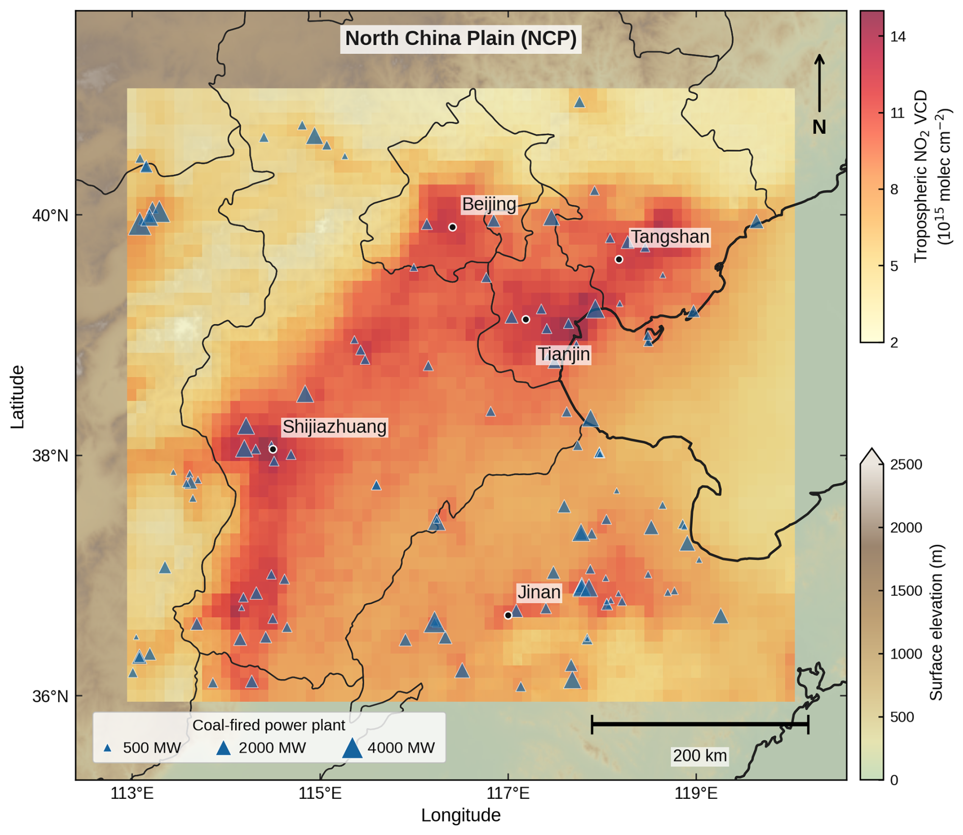
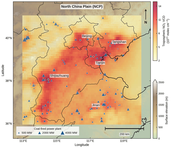
Figure 1Study region. A shaded-relief map of the North China Plain (lower colour bar: surface elevation) overlaid with the 2023 TROPOMI annual-mean tropospheric NO2 column after quality screening (upper colour bar). Triangles mark the 126 coal-fired power plants of the Global Power Plant Database within the study domain, with area directly proportional to installed capacity (60–4520 MW). Major cities and a 200 km scale bar are annotated.
Existing emission-inversion methods all face some degree of limited applicability over the North China Plain (Martin et al., 2003; Streets et al., 2013). The flux-divergence method (FDM; Beirle et al., 2011, 2019; de Foy et al., 2015; Liu et al., 2016) relies on assumptions of uniform wind and a clean background, and its signal-to-noise ratio is too low under the high background concentrations and dense sources of the NCP. A quantitative analysis shows that in winter (December–February), the domain-mean wind speed is about 0.95 m s−1, the characteristic plume scale is about 24 km, the interquartile range of the background vertical column density (VCD) is as large as 100 µmol m−2, and the median nearest-neighbour distance among the 126 coal-fired power plants within the domain is only 14 km, so none of the three necessary conditions is met (Fig. S5). Global chemical-transport-model (CTM) data assimilation (Miyazaki et al., 2012, 2021) represents transport and chemistry in full but is computationally expensive, with typical run times of hundreds of CPU hours per year; the fast regional inversion DECSO (Daily Emission estimates Constrained by Satellite Observations; Mijling et al., 2013) is suitable at moderate resolution but lacks the fast, end-to-end inference capability afforded by deep learning.
In recent years, methods that combine physical constraints with data-driven inference, such as physics-informed neural networks (PINNs), differentiable simulation and simulation-based inference, have developed rapidly in Earth system science (Raissi et al., 2019; Cranmer et al., 2020; Karniadakis et al., 2021). PINNs embed physical laws into the training of neural networks, so that network outputs remain physically consistent even under sparse-data or label-free conditions. For NOx, Xing et al. (2022) inferred emissions from satellite-derived surface NO2 with a physically informed variational autoencoder trained on chemical-transport-model simulations, and Chen et al. (2026) estimated regional and point-source emissions across China directly from TROPOMI with a directional-derivative approach. Here we extend this idea to atmospheric NOx emission inversion: a differentiable transport-chemistry operator is embedded as a fixed decoder within an autoencoder, so that the neural encoder can infer an emission field under the physical constraint of reconstructing the satellite observations, without any emission labels. To our knowledge, such a label-free combination of a differentiable forward operator with neural-network inversion, together with a systematic comparison of different neural backbones (Ronneberger et al., 2015), the Fourier neural operator (Li et al., 2020), and their spectral fusion, has not yet been applied to high-resolution NOx emission inversion. We emphasize that our framework differs in mechanism from the classical PINN: a PINN approximates the solution of a partial differential equation (PDE) with a neural network and uses the PDE residual as a soft-constraint loss term, whereas our framework retains a simplified numerical solver of transport and first-order decay as a fixed, differentiable decoder and treats physics as a hard constraint, with the neural network performing only the amortized inverse mapping from observations to emissions (after training, a single forward pass suffices for inference, with no per-day re-optimization). It is therefore closer to the differentiable-simulation and inverse-rendering paradigm.
We present the PINE-NOx framework (Fig. 2), which we position as a physics-constrained neural inversion for atmospheric inverse problems: the neural encoder infers emissions from TROPOMI columns, the fixed, differentiable advection-chemistry operator serves as a decoder that renders emissions into columns, and the network is trained label-free to reconstruct the observed columns. The paper makes three contributions. (1) End-to-end and label-free: it does not rely on any existing emission-inversion product as supervision; emissions are inverted directly as a physical latent variable, avoiding the circularity of training on inventory-derived labels. (2) It systematically compares convolutional, spectral-operator and spectral-fusion encoder backbones in terms of their forward skill under label-free physical reconstruction, providing a basis for architecture selection in this class of inverse problems. (3) It compares the retrieved pattern with the EDGAR allocation over the NCP, with an uncertainty budget and a synthetic test with known emissions that shows which part of the change the method produces on its own, and tests the pattern against the MEIC inventory and a WRF-Chem simulation with surface stations; once trained, inference takes milliseconds.
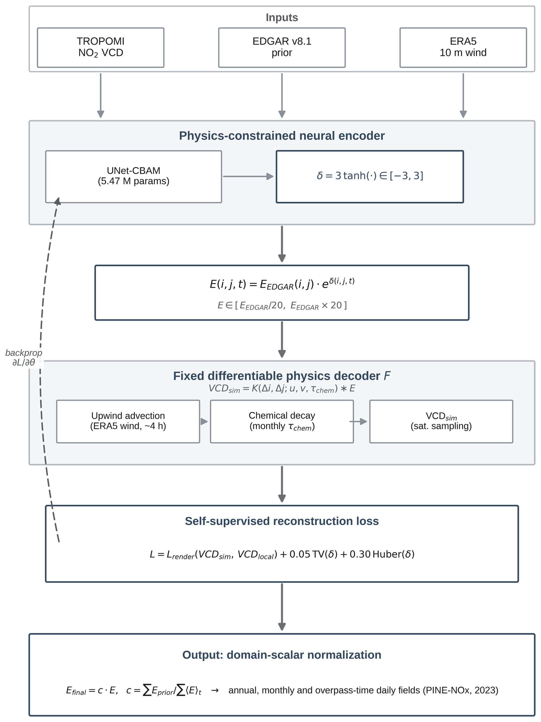
Figure 2Schematic of the physics-constrained inverse neural estimation (PINE-NOx) framework.
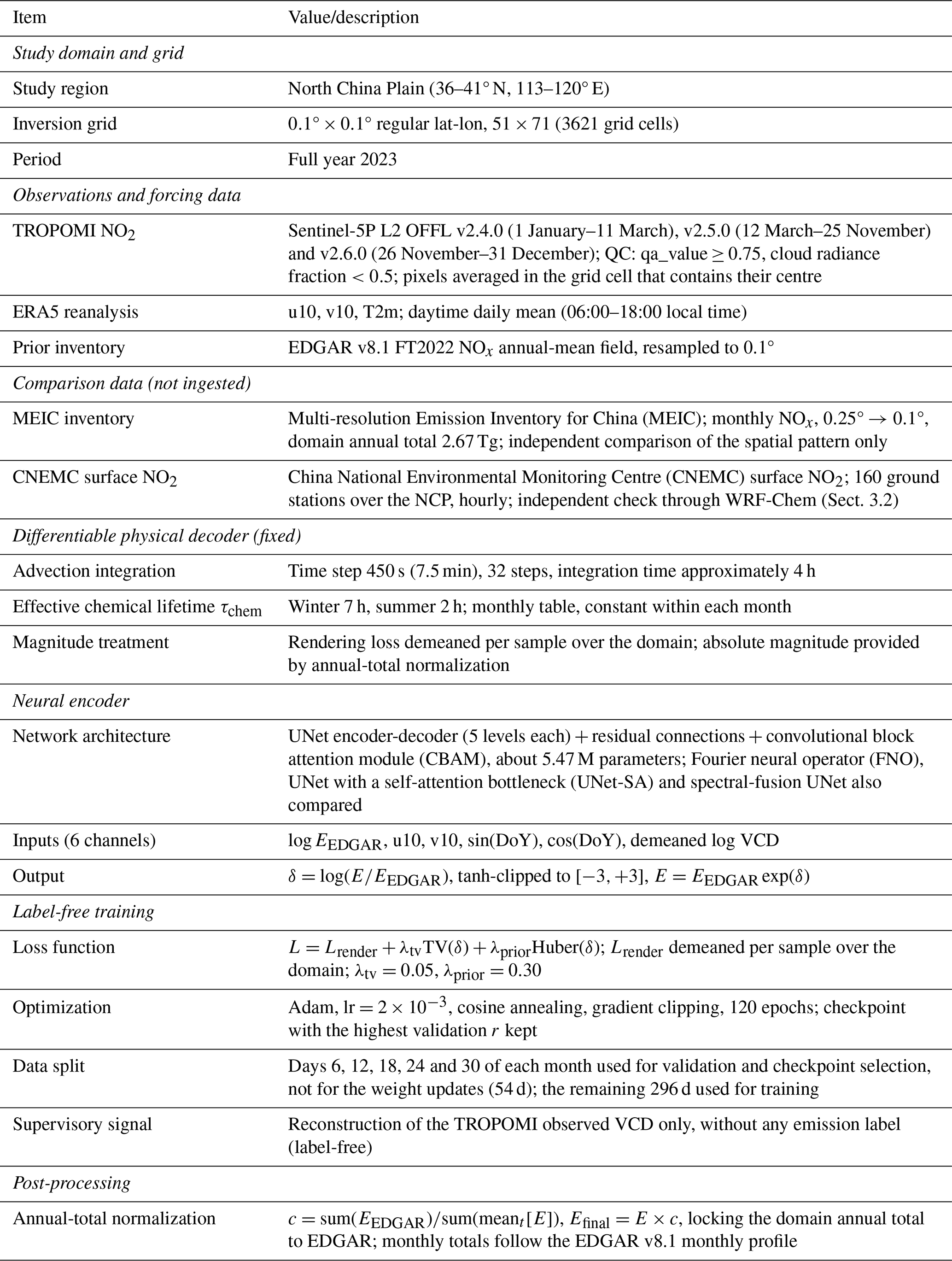
The observational and reanalysis data, the prior emission inventory, and the key configuration parameters of PINE-NOx used in this paper are summarized in Table 1.
Table 1Summary of PINE-NOx data sources and key configuration parameters.
2.1 Study region and observational data
The study region is the core of the North China Plain (36–41° N, 113–120° E; Fig. 1), discretized on a 0.1°×0.1° regular latitude–longitude grid (51×71 grid cells). Satellite observations are taken from the Sentinel-5P/TROPOMI tropospheric NO2 VCD product (Veefkind et al., 2012; Boersma et al., 2018; van Geffen et al., 2022), quality-controlled with qa_value ≥ 0.75 and cloud radiance fraction<0.5, and gridded by averaging the pixels whose centres fall in each grid cell (the seasonal-mean spatial distribution is shown in Fig. 3 and the monthly-mean valid-pixel coverage in Fig. S1 in the Supplement). The 2023 record spans three processor versions (Table 1). Version 2.5.0 changes only the quality flag over snow and ice. In version 2.6.0 a change in the cloud retrieval affects the cloud pressure and hence the air mass factor. Omitting the 33 retrieval days of version 2.6.0 changes the annual pattern by 1.1 % of the emissions. All December days are from version 2.6.0; the December pattern differs from the January pattern by 13.1 %, close to the 11.3 % between February and January. Retrieval uncertainties of the tropospheric NO2 column, which are dominated by the tropospheric air mass factor, have been characterized in detail elsewhere (Boersma et al., 2004; Lorente et al., 2017). Meteorological forcing is from the ERA5 hourly reanalysis (Hersbach et al., 2020), from which we extract daytime daily means (06:00–18:00 local time) of the 10 m wind field (u10, v10) and the 2 m surface air temperature. The prior emission inventory is the EDGAR v8.1 (Crippa et al., 2026) annual-mean NOx field, resampled to 0.1° resolution with area-conservative regridding and used as the prior base for the physical reconstruction, as the Huber reference constraint, and as an input feature to the neural encoder.
Two further datasets are used solely for evaluation and at no stage enter the inversion as a prior, a label or a constraint. The Multi-resolution Emission Inventory for China (MEIC; Zheng et al., 2018; Li et al., 2017) provides a bottom-up, sector-resolved monthly NOx inventory, regridded from 0.25° to the 0.1° study grid (domain annual total 2.67 Tg; NOx masses are given as NO2-equivalent mass for all inventories in this paper); because it is constructed independently of TROPOMI and of EDGAR, it is used only to test whether the inverted spatial pattern moves towards or away from an independent bottom-up estimate (Sect. 3.3). Hourly surface NO2 observations from 160 China National Environmental Monitoring Centre (CNEMC) stations within the study domain are used to evaluate WRF-Chem simulations driven by the different emission fields (Sect. 3.2) and are compared directly with the emissions in the station cells in Fig. S6.
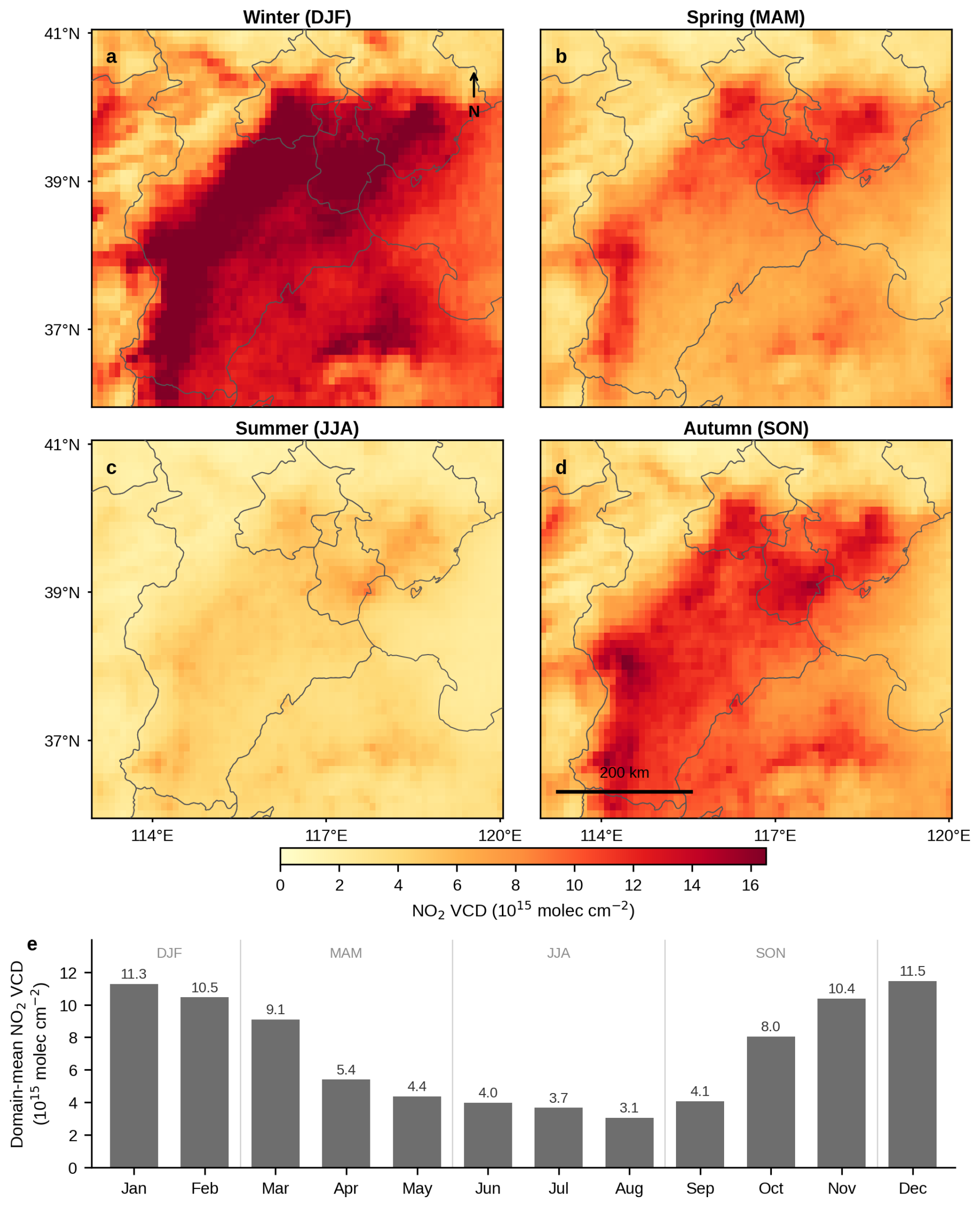
Figure 3Seasonal climatology of the TROPOMI-observed tropospheric NO2 column over the North China Plain (2023). (a–d) Winter, spring, summer and autumn means; (e) monthly variation of the regional mean.
2.2 Differentiable atmospheric transport-chemistry decoder
The differentiable physical decoder describes the spatial distribution of the NO2 VCD formed by a given NOx emission field E(i,j) after atmospheric advection and chemical decay, and serves as the fixed decoder F in the physics-constrained autoencoder. The decoder solves the advection-decay equation in a two-dimensional Eulerian framework: starting from a zero-column initial condition, at each time step it successively applies the local emission source term, the upwind advection term and the first-order chemical-decay term to the column field and integrates iteratively, finally yielding the locally driven simulated column field VCDsim=F(E). The upwind scheme is differentiable throughout while ensuring numerical stability, and a non-negativity constraint is imposed on the column after each step. The driving wind is the ERA5 daytime daily-mean 10 m wind field (u10,v10); the integration time step is 450 s (about 7.5 min) over 32 steps (an integration time of about 4 h, comparable to the typical NOx chemical lifetime). The effective NO2 chemical lifetime τchem follows a monthly-mean parameterization based on the seasonal variation of OH (7, 6, 5, 4, 3, 2, 2, 2, 4, 4, 5 and 7 h from January–December, spatially uniform and constant within each month). These are daytime lifetimes near the overpass time. They are of the same magnitude as satellite-derived lifetimes in China: 2.5–6.4 h for five North China Plain cities in May to September (Liu et al., 2016) and, at noon over Wuhan, 1.4 h in summer and 4.8 h in winter (Zhang et al., 2023). No monthly series has been published for the NCP, so the values for the transitional months were set by hand between the winter and summer values. The operator is thus a simplified transport–decay model: it uses one daytime-mean wind, a spatially uniform lifetime and a fixed conversion, and it does not resolve vertical mixing or nonlinear chemistry; the sensitivity of the results to the lifetime, the integration time and the wind level is part of the uncertainty budget (Sect. 3.3). On the observation side, the TROPOMI column is decomposed into a uniform inflow background and a local emission signal: the background field VCDbg is estimated as the median of valid pixels in a four-cell-wide border along the edges of the study domain (approximating the uniform background of long-range upwind transport), and the local emission signal is the target to be reconstructed by the decoder. Because the decoder is fully differentiable, the reconstruction error can be differentiated with respect to the emission field E, providing the analytical gradients required for end-to-end training of the neural encoder (see Sect. 2.3). We note that the decoder drives the transport of a single-overpass snapshot with the ERA5 daytime-mean 10 m wind during the satellite overpass window and does not explicitly represent intraday wind-direction changes; the sensitivity to the width of the background border (three and five cells instead of four) is part of the uncertainty budget (Sect. 3.3).
2.3 Neural encoder and self-supervised training based on differentiable physics
Emission inversion in PINE-NOx is performed by a neural encoder. The encoder takes a six-channel spatial field as input: log (EEDGAR), the ERA5 wind components u10 and v10, the sine and cosine encodings of the day-of-year (sin (DoY),cos (DoY)), and the domain-mean-removed log of the TROPOMI VCD. It outputs a log-increment field δ(i,j), clipped by tanh to [] (corresponding to emissions in ), from which the emissions are obtained as in Eq. (1). The specific encoder backbone is systematically compared in Sect. 3.1; the main results of this paper use UNet-CBAM, whose CBAM attention module follows Woo et al. (2018). The emissions output by the encoder are immediately fed into the fixed, differentiable decoder F to generate the simulated column VCDsim, and the network is trained with reconstruction of the observations as its sole objective, with the loss function given in Eq. (2). Here the rendering term , TV(δ) is a total-variation spatial-smoothness regularizer, and H(δ) is a Huber regularizer referenced to the EDGAR prior; after sensitivity testing we set λtv=0.05 and λprior=0.30 (Fig. S9). Cells whose observed column does not exceed the boundary background (31 % of the valid cell-days) carry no local signal and are left out of the rendering term. Because the decoder is differentiable, the gradient of the reconstruction error is back-propagated end-to-end to the encoder weights, so that the network learns to invert emissions without ever seeing any emission label; this is how the physics-constrained autoencoder learns. Training uses Adam (Kingma and Ba, 2015) with gradient clipping for a fixed 120 epochs, and the network state after the epoch with the highest reconstruction r on the validation days is kept (the checkpoint; epoch 57 of 120 for UNet-CBAM and epoch 5 for FNO, Table 2); inference takes about 5 ms per day on our experimental platform. The data are split with a fixed hold-out validation set: days 6, 12, 18, 24 and 30 of each month (54 d) are excluded from the weight updates and used only to select the checkpoint, and the remaining 296 d are used for training; generalization to unseen seasons is tested separately by leaving out one whole season at a time (Fig. S7). The validation days are interleaved in time with the training days, and the evaluation metric is the demeaned log-space correlation (characterizing the spatial pattern rather than pointwise magnitude), so the temporal autocorrelation between training and validation days has limited influence on the conclusions. This training is a self-supervised paradigm: reconstruction of the observed VCD itself serves as the supervisory signal, and no emission inventory is used as a label at any stage (i.e. label-free).
Table 2Comparison of PINE-NOx encoder architectures. Overall forward r: mean daily log-space spatial correlation between the decoder-simulated and the background-removed TROPOMI columns over all 347 evaluated days; held-out forward r: the same over the 54 validation days (days 6, 12, 18, 24 and 30 of each month), which were not used to fit the weights but were used to select the checkpoint (epochs 57, 85, 67 and 5 of 120 for the four backbones as listed); Δr: overall forward r minus that of EDGAR (0.331; 0.332 on the held-out days).

2.4 Identifiability and regularization analysis of the physical constraint
This section describes, in terms of inverse-problem theory, the constraint that the fixed, differentiable decoder F imposes on emission inversion, providing the theoretical basis for the improvement in reconstruction skill and for the prior-removal experiment in Sect. 3.1. In short, differentiable physics does not provide a higher-accuracy forward approximation; rather, it transforms an intrinsically ill-posed, over-parameterized inverse mapping into a constrained deconvolution problem that is physically anchored in the observable subspace and closed by the prior in the unobservable subspace.
-
Linear structure of the decoder. The transport-chemistry decoder used here is a linear operator on the emission field E. Its discrete evolution follows ), where Am is the combined monthly upwind-advection and first-order chemical-decay operator and the initial column is zero. Expanding step by step and summing over time, the simulated column can be written in the compact form of Eq. (3), where the transport-decay kernel is given in Eq. (4), a linear operator depending only on the wind field and the chemical lifetime. Thus, inverting the emissions E from an observed VCDTROP reduces mathematically to a deconvolution problem for the linear operator Km, rather than nonlinear optimization in the general sense.
-
Ill-posedness of the inverse problem. As an advection-decay smoothing operator, Km imposes a spatial low-pass action on the emission field: high-frequency spatial structure is strongly attenuated in the forward mapping to columns, so the singular-value spectrum of Km decays rapidly and forms an approximate null space. Therefore, directly inverting from a finite, noisy VCDTROP is a typical ill-posed problem, and neither fine-scale spatial structure nor the absolute emission magnitude can be uniquely determined by the observations. PINE-NOx does not invert directly; instead, it regularizes in a variational physical-likelihood-plus-prior form, injecting controllable constraints along the ill-posed directions.
-
Amortized maximum-a-posteriori estimation. For the observation of any given day, the ideal regularized inversion corresponds to the maximum-a-posteriori (MAP) objective of Eq. (5), where Ω is the valid-observation mask, TV is the total-variation prior, and H is the Huber prior on the log deviation δ from EDGAR. Rather than solving this optimization separately for each day, PINE-NOx trains a single neural encoder gθ that outputs , amortizing the MAP solution over all days with one shared network. In this framework the encoder approximates the posterior mode, the fixed differentiable physics provides the analytical gradient of the likelihood term, and the prior term provides regularization, the three being co-optimized through end-to-end back-propagation.
-
Identifiability decomposition. The above framework partitions the emission degrees of freedom into two complementary subspaces. The first is the observable subspace, namely the spatial modes spanned by the row space of Km that contribute significantly to the column; this subspace is directly anchored by the physical-likelihood term, and its inversion is determined by the TROPOMI observations through the differentiable physics, without relying on any existing emission-inversion product as a label; it therefore also inherits the structural errors of the simplified operator. The second is the unobservable subspace, namely the fine-scale structure that falls into the approximate null space of Km together with the overall magnitude; this subspace is nearly indistinguishable in the observations and is instead closed by the prior: the total-variation prior suppresses non-physical high-frequency oscillations, the Huber prior softly anchors it to the spatial structure of EDGAR, and the overall absolute magnitude is finally calibrated by the single domain-wide scalar normalization of Sect. 2.5.
-
Immunity to rank-one perturbations through mean-centring. The rendering loss removes the domain-wide mean from both the simulated and the observed VCD, which is equivalent to orthogonally projecting out the rank-one perturbation subspace spanned by overall gain and background from the data term. The physical meaning is that an error in the absolute value of the chemical lifetime τchem manifests mainly as an approximately multiplicative overall scaling of the column, whereas an error in the regional background estimate manifests mainly as an additive overall shift; both are eliminated to first order by demeaning. The loss function is therefore first-order invariant to τchem calibration error and background-estimation error, making the inverted spatial pattern insensitive to these two systematic uncertainties, a property confirmed empirically by the τchem sensitivity experiment in Sect. 4.1 (the spatial correlation is essentially unchanged even when the lifetime is perturbed by several-fold; Fig. S2). The same invariance means that the domain-wide emission level is not constrained by the observations at all: multiplying all emissions by a constant leaves the loss unchanged, so the level is set only by the prior term and, in the final product, by the normalization of Sect. 2.5.
The role of the fixed differentiable physics is therefore to reconstruct an over-parameterized inverse mapping, one prone to degenerating into an image memorization of the observations, into a constrained deconvolution that rewards likelihood only for emissions consistent with physical transport; the prior and the domain-wide normalization then close the null-space directions that the observations cannot identify. This identifiability structure, namely a relative spatial pattern adjusted by the observations and physics around a prior that sets the absolute magnitude and the large-scale structure, is the theoretical basis on which PINE-NOx can improve the reconstruction of the observed column pattern (Sect. 3.1) without using any emission label, and it defines what the later comparisons can test: the spatial pattern, not the totals. Because the operator is simplified, part of the retrieved pattern can come from the method itself; Sect. 3.3 estimates this part with a synthetic test with known emissions.
2.5 Domain-wide annual-total emission normalization
The rendering loss of the neural encoder removes the domain-wide mean from both the simulated and the observed VCD, so it constrains only the relative spatial pattern of emissions and contains no absolute-magnitude information; the network's inverted emissions thus have an overall-magnitude degree of freedom. To provide an absolute-magnitude reference, a single domain-wide scalar annual-total normalization is introduced as a design constraint, as in Eq. (6) (c≈1.27 in this study). This normalization only locks the domain's annual total emission to EDGAR and does not change the relative spatial pattern (the independence of this normalization from the spatial pattern is shown in Fig. S8). Monthly totals of the product follow the EDGAR v8.1 monthly profile for 2022, built from the EDGAR sector maps and the sector-specific monthly fractions for China (winter-to-summer ratio 1.09), so that annual and monthly totals come from one inventory. Normalizing to the MEIC total instead (0.88 of the EDGAR total) would rescale every field by the same factor and leave all patterns, shares and correlations unchanged. The lower MEIC 2023 total is consistent with the continued decline of NOx emissions after 2022, although the two inventories also differ in method; the inversion cannot correct the EDGAR total for this decline, because the domain level is not constrained by the observations. Because the normalization is a single domain-wide constant, all log-space correlations and log-RMSE values are mathematically strictly unaffected by its value ( is merely a constant shift); hence the agreement of the annual total with EDGAR is a design constraint on the absolute magnitude rather than an independent validation. What can be tested is the reconstruction of the observations (an internal check, Sect. 3.1), the consistency of the pattern in a CTM (WRF-Chem, Sect. 3.2) and the comparison of the pattern with MEIC, judged against a synthetic test with known emissions (Sect. 3.3).
3.1 Encoder architecture comparison and observation reconstruction
Within a unified label-free physical-reconstruction framework, the spatial consistency between the forward-decoder-simulated VCD and the background-removed TROPOMI column (VCDlocal, Sect. 2.2) was evaluated with the log-space Pearson correlation coefficient over the cells whose observed column exceeds the boundary background; the correlation was computed on all 347 d with at least 50 evaluated cells, without using any emission label at any stage. Driving the decoder with the EDGAR annual-mean emissions, the spatial correlation between the simulated VCD and the observations averages only r=0.331, reflecting the inherent limitation of a static annual-mean inventory in representing day-to-day spatial patterns. Within this framework we systematically compare the forward skill of four neural-encoder backbones (Fig. 4a, Table 2): UNet-CBAM (5.47 M parameters, r=0.871), spectral-fusion UNet (6.53 M, r=0.884), UNet-SA (6.27 M, r=0.874) and the Fourier neural operator FNO (2.10 M, r=0.821). On the 54 validation days alone, which were not used to fit the weights but were used to select the checkpoint, the values are 0.856, 0.859, 0.855 and 0.795, against 0.332 for EDGAR (Table 2); because the checkpoint maximizes the skill on these days, they are not an independent test set. All four backbones far exceed the EDGAR prior and differ very little from one another (0.821–0.884), indicating that, under a unified random seed, training under the differentiable-physics constraint is insensitive to the encoder architecture (seasonally stratified cross-validation further supports the seasonal stability of this skill; Fig. S7). UNet-CBAM was retained as the production backbone (, 95 % interval 0.528–0.553 from a bootstrap over days; Fig. S13). The spectral-fusion UNet scores slightly higher (0.884), but this difference lies within the spread of UNet-CBAM itself across four network initialisations (0.871–0.886). The annual emission patterns obtained with the spectral-fusion UNet and with UNet-SA differ from the UNet-CBAM pattern by 1.3 % and 1.4 % of the emissions at 0.5° (fraction of the total emission placed in different 0.5° cells; Sect. 3.3), no more than the patterns of the four UNet-CBAM initialisations differ from one another (0.7 %–1.5 %), so the results of Sect. 3.3 do not depend on this choice; UNet-CBAM is used for all sensitivity runs of the uncertainty budget. Unlike the multi-step paradigm of first solving the inversion day by day and then training a network to fit it, here all backbones are trained end-to-end with the same physical-reconstruction objective and ranked by their forward skill against the observations (rather than by their fidelity to an existing inversion product), so the comparison does not depend on any existing inversion product. We emphasize that this correlation is a spatial-pattern skill after demeaning in log space; the network targets reconstruction of the observed pattern and does not constrain absolute magnitude, so a magnitude-sensitive absolute RMSE is not used as the primary metric here. We also note that the forward skill above is computed with the same differentiable decoder used in training and is therefore an internal self-consistency metric of observation reconstruction, not a validation of the emissions; consistency checks outside the training decoder use the WRF-Chem simulation in Sect. 3.2 and the MEIC inventory in Sect. 3.3.
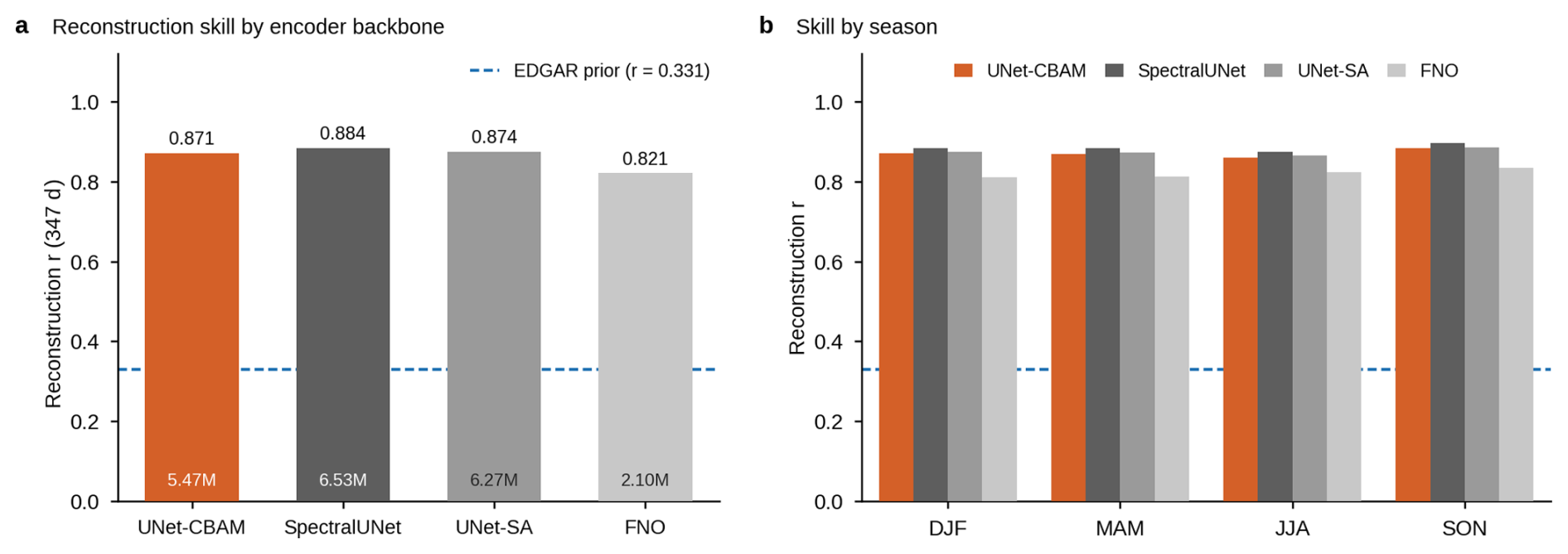
Figure 4Encoder-backbone ablation. The forward reconstruction skill r is defined as the spatial correlation coefficient between the simulated column rendered by the physical decoder and the background-removed TROPOMI column in log space, on cells above the boundary background, averaged over 347 d. (a) Overall skill of the four encoder backbones, with the parameter count annotated within each bar, against the EDGAR prior baseline (r=0.331); (b) the same skill decomposed by season.
Figure 5 illustrates the multi-season forward self-consistency of the inverted emissions for three representative days: a clean summer day (10 August 2023), a transitional autumn day (7 October 2023) and a polluted winter day (18 December 2023). On each day, the simulated columns obtained by driving the decoder with the daily PINE-NOx emissions reproduce the TROPOMI observed morphology () markedly better than the unadjusted EDGAR prior (), with the improvement holding consistently under both clean and polluted conditions. Extending the skill to the full year (Fig. 6), the monthly forward correlation of the PINE-NOx-inverted emissions is systematically higher than that of the prior, and the annual-mean skill over all 347 d rises from 0.331 for EDGAR to 0.871. The seasonal means are 0.871 in winter (DJF), 0.869 in spring (MAM), 0.860 in summer (JJA) and 0.883 in autumn (SON), and when a whole season is withheld from training the skill on that season is still 0.841–0.859 (Fig. S7), so the reconstruction skill does not depend on a particular season. This robustness is consistent with the constraint of the fixed physical decoder on the advection-chemistry processes and the seasonal chemical-lifetime parameterization, which allow the encoder to generalize without season-specific tuning.
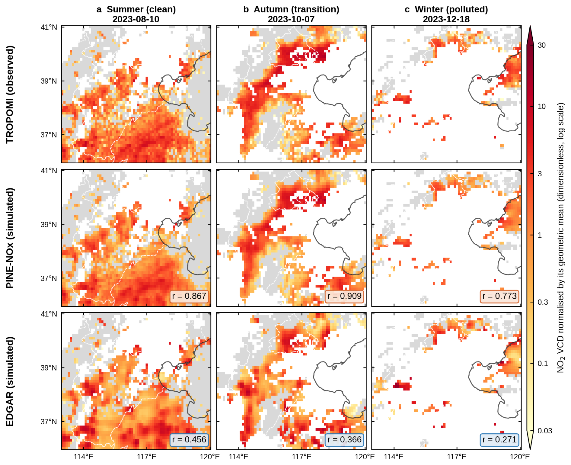
Figure 5Multi-season forward self-consistency of the inverted emissions. Each column is one of three representative days spanning the seasonal range of the North China Plain: (a) a clean summer day (10 August 2023), (b) a transitional autumn day (7 October 2023) and (c) a polluted winter day (18 December 2023). From top to bottom, the rows are: the TROPOMI observed tropospheric NO2 column (background removed), the column simulated by the differentiable transport-chemistry decoder driven by the daily PINE-NOx emissions, and the column simulated under the unadjusted EDGAR prior. Each field is divided by its geometric mean; grey cells are valid observations that do not exceed the boundary background. The value in each cell of the lower two rows is the log-space spatial Pearson correlation between the simulated and observed columns for that day. White dashed lines are provincial boundaries.
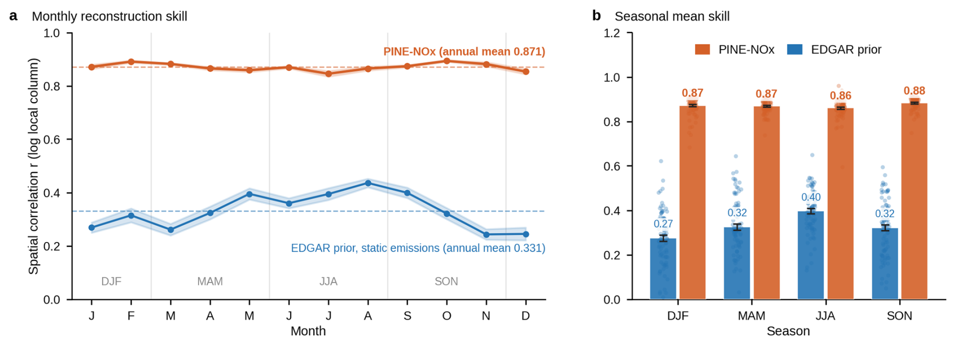
Figure 6Forward-simulation skill of the inverted emissions over the full year (347 d). The skill r is defined as the log-space spatial Pearson correlation between the forward simulation and the background-removed TROPOMI NO2 column, on cells above the boundary background. (a) Monthly-mean r for PINE-NOx (orange) and the EDGAR prior (blue); the shaded band is the ±1 standard error of the daily values within each month, and the dashed lines give the annual-mean skill. The EDGAR emissions are fixed; their r varies with the daily wind, the monthly lifetime and the observation sampling. (b) Season-aggregated mean skill; bars are seasonal means, whiskers are ±1 standard error, and dots are single-day values.
To directly address the central question of whether the spatial-pattern improvement arises solely from the EDGAR prior structure, we designed a prior-removal experiment: when the Huber reference prior is replaced from the real EDGAR spatial field by a uniform prior stripped of all spatial information (a flat, domain-wide constant prior), the spatial correlation between the network's inverted forward VCD and TROPOMI is not reduced (0.909 against 0.871; Fig. S9) and changes little across a sweep of λprior (0.855–0.910). Because a uniform prior contains no spatial information, the reconstruction skill does not rest on the prior. The emission pattern itself does depend on the prior (log-space r=0.83 between the annual fields obtained with the flat and with the EDGAR prior), and this dependence is carried as a separate term of the uncertainty budget (Sect. 3.3).
3.2 WRF-Chem consistency check
The forward self-consistency evaluations above are all based on the same differentiable decoder used in the inversion; to provide an external reference independent of that decoder, we carried out a WRF-Chem three-dimensional forward-simulation experiment (5–31 July 2023, about 27 d simulated, of which the first 3 are spin-up and 8–31 July (24 d) are analysed; 27 km horizontal resolution, the RADM2 gas-phase chemical mechanism with the SORGAM aerosol module, chemical initial and boundary conditions from the CAMS EAC4 reanalysis; full configuration in Table S1 in the Supplement), driven separately by the EDGAR prior and by the PINE-NOx-inverted emissions, and in addition by MEIC, by EDGAR smoothed with a 2-cell Gaussian kernel and by PINE-NOx obtained with the MEIC prior. All runs share the same configuration and the same NOx total within the domain, so only the spatial pattern of the emissions differs (a comparable WRF-Chem–TROPOMI NO2 cross-evaluation strategy is used by Poraicu et al., 2023). Taking the TROPOMI overpass time (about 13:30 local solar time) as the temporal reference, we computed the monthly-mean tropospheric NO2 VCD over the NCP for 8–31 July 2023 and compared it with TROPOMI observations at the pixel scale, applying the TROPOMI averaging kernels (Fig. 7). With equal totals, all runs reproduce the domain-mean column within 4 %. The spatial pattern of the July-mean column moves closer to TROPOMI with PINE-NOx emissions (log-space r=0.925 against 0.876 for EDGAR; difference +0.049, 95 % interval 0.036–0.061), and so does the day-to-day pattern (0.735 against 0.696). Surface NO2 at the 160 CNEMC stations gives a different picture. Averaged over all hours of the 15 dry days (the 24 analysed days without the 9 d on which the ERA5 precipitation averaged over the stations reached 5 mm, excluded because the runs include no wet scavenging; this screening rule was defined after a first inspection of the daily station results; Table S1), the across-station correlation is the same for both runs (0.268 and 0.266; difference +0.002, ), and in the 13–15 China Standard Time (CST) window it is lower with PINE-NOx than with EDGAR (0.310 against 0.439; difference −0.129, −0.187 to −0.036, 0.5° spatial-block bootstrap). All runs underestimate afternoon surface NO2 by 44 %–52 %, which points to a shared model error in boundary-layer mixing. A cruder test without a transport model does not favour the new pattern either: across the stations, July-mean surface NO2 correlates slightly better with the EDGAR emissions in the station cells than with PINE-NOx (log-space r=0.365 against 0.306; Fig. S6). The WRF-Chem experiment is an external CTM-based consistency check: it is independent of the inversion decoder but not of the observations, because the constraint reference used by WRF-Chem (TROPOMI NO2 VCD) is the same source as the observations used in the PINE-NOx inversion, so the column comparison shows consistency with the observations the inversion was fitted to, within a different transport model; only the station comparison is independent, and in this one month and one model configuration it does not show the PINE-NOx pattern to be better than EDGAR. In addition, this experiment covers only 24 analysed days after a 3 d spin-up from CAMS EAC4 initial conditions; the averaging kernel changes the EDGAR- and PINE-NOx-driven columns by almost the same factor (Fig. S11). An independent emission validation still depends on non-satellite observations such as aircraft and ground-based flux measurements, which we leave for future work (Cooper et al., 2017; Goldberg et al., 2022).
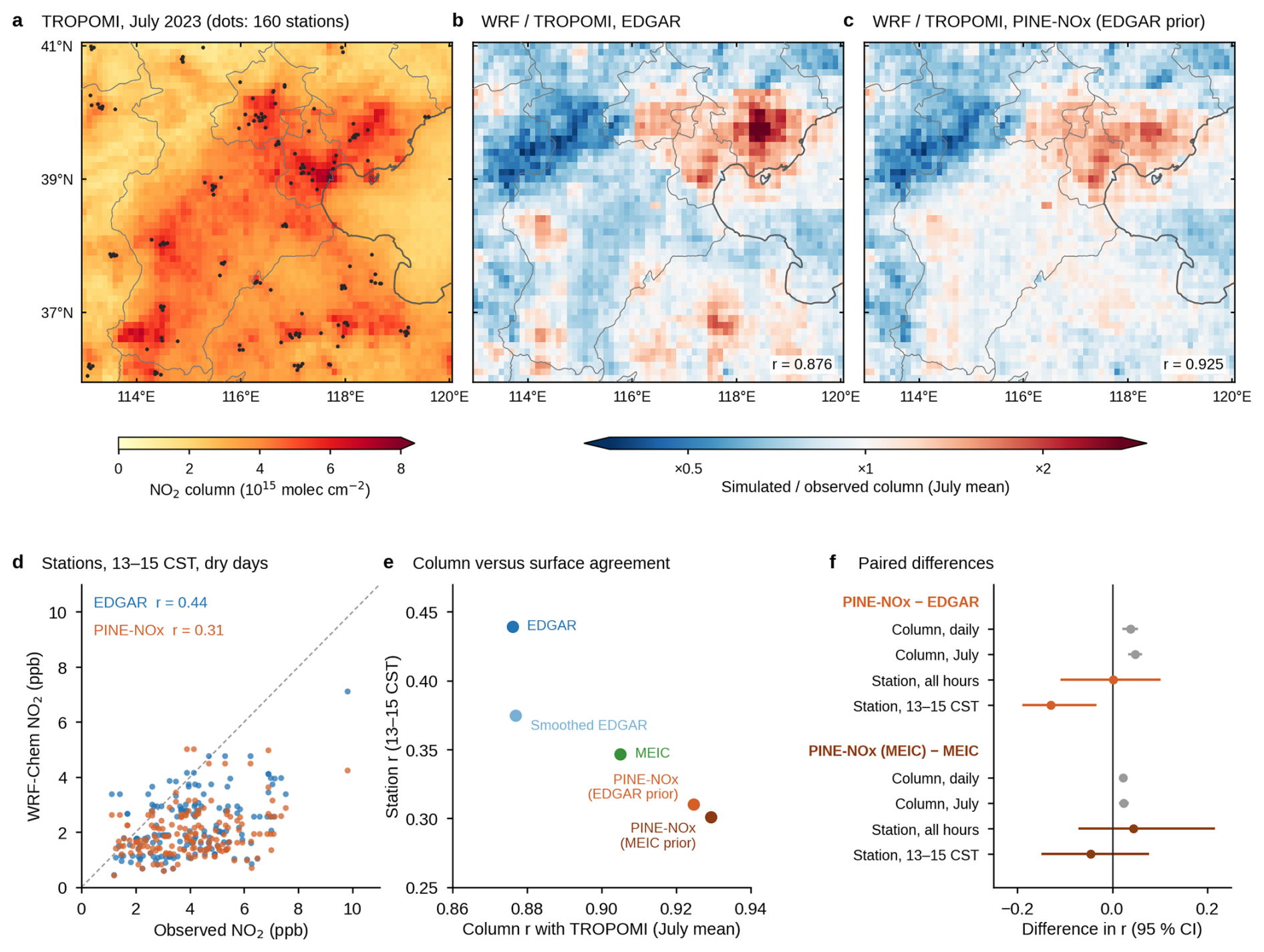
Figure 7WRF-Chem consistency check, 8–31 July 2023. All runs use one WRF-Chem configuration with equal in-domain NOx totals; only the spatial pattern of NOx emissions differs. (a) TROPOMI July-mean NO2 column at overpass; dots mark the 160 CNEMC stations. (b, c) Ratio of the simulated (averaging kernels applied) to the observed July-mean column for EDGAR and for PINE-NOx with the EDGAR prior, with the log-space spatial r. (d) Simulated against observed surface NO2 at the stations, 13–15 CST means on 15 dry days, with Pearson r (one station per run above 11 ppb not shown). (e) Column r with TROPOMI against station r for EDGAR, EDGAR smoothed with a 2-cell Gaussian kernel, MEIC and PINE-NOx with the EDGAR and the MEIC prior. (f) Paired differences in r with 95 % intervals (column: bootstrap over days; stations: 0.5° spatial-block bootstrap, 2000 draws). The column comparison is not independent of TROPOMI, which PINE-NOx was fitted to; the station comparison is.
3.3 Spatial pattern of NOx emissions over the North China Plain
Relative to EDGAR, PINE-NOx places less of the emissions in the urban–industrial cores and more in their surroundings (Fig. 8). In the PINE-NOx field, the 10 % of grid cells with the highest EDGAR emissions hold 35 % of the domain total, against 59 % in EDGAR, and the half of the cells with the lowest EDGAR emissions hold 16 %, against 6 %. A synthetic test with known emissions shows that a change of this size also arises from the method itself (Sect. S1, Table S2). In this test, WRF-Chem columns simulated from EDGAR for July and January (with a simpler model configuration than in Sect. 3.2, given in Sect. S1) were sampled with the daily TROPOMI valid-pixel mask and inverted with the same networks, so the true emissions equal the prior. The share of the 10 % highest-emitting EDGAR cells nevertheless fell by 21 percentage points in July and 26 points in January, against 20 and 25 points for the observed columns on the same days, and the share of the lowest-emitting half rose by 9 and 12 points (8 and 11 observed). The retrieved concentration also depends little on the true one: with the MEIC pattern as the true field, whose top-10 % share is 30–31 points lower than that of EDGAR, the retrieved share was only 2 points lower than in the test with EDGAR as the true field. The shift of emission out of the EDGAR cores is therefore primarily a structural artefact of the method, not an independently observed redistribution. Its most likely source is the two-dimensional decoder, which describes transport and chemistry as advection with first-order loss in a single layer and cannot reproduce the vertical mixing and the non-linear chemistry of the three-dimensional model. We use these shares only to describe the PINE-NOx field. For the same reason, the 64 of the 98 0.5° blocks in which the change exceeds twice its 1σ uncertainty (dots in Fig. 8a; blocks whose 25 cells all lie in the mask of the uncertainty budget) are not evidence of an observed change, because the budget below does not contain this structural term.
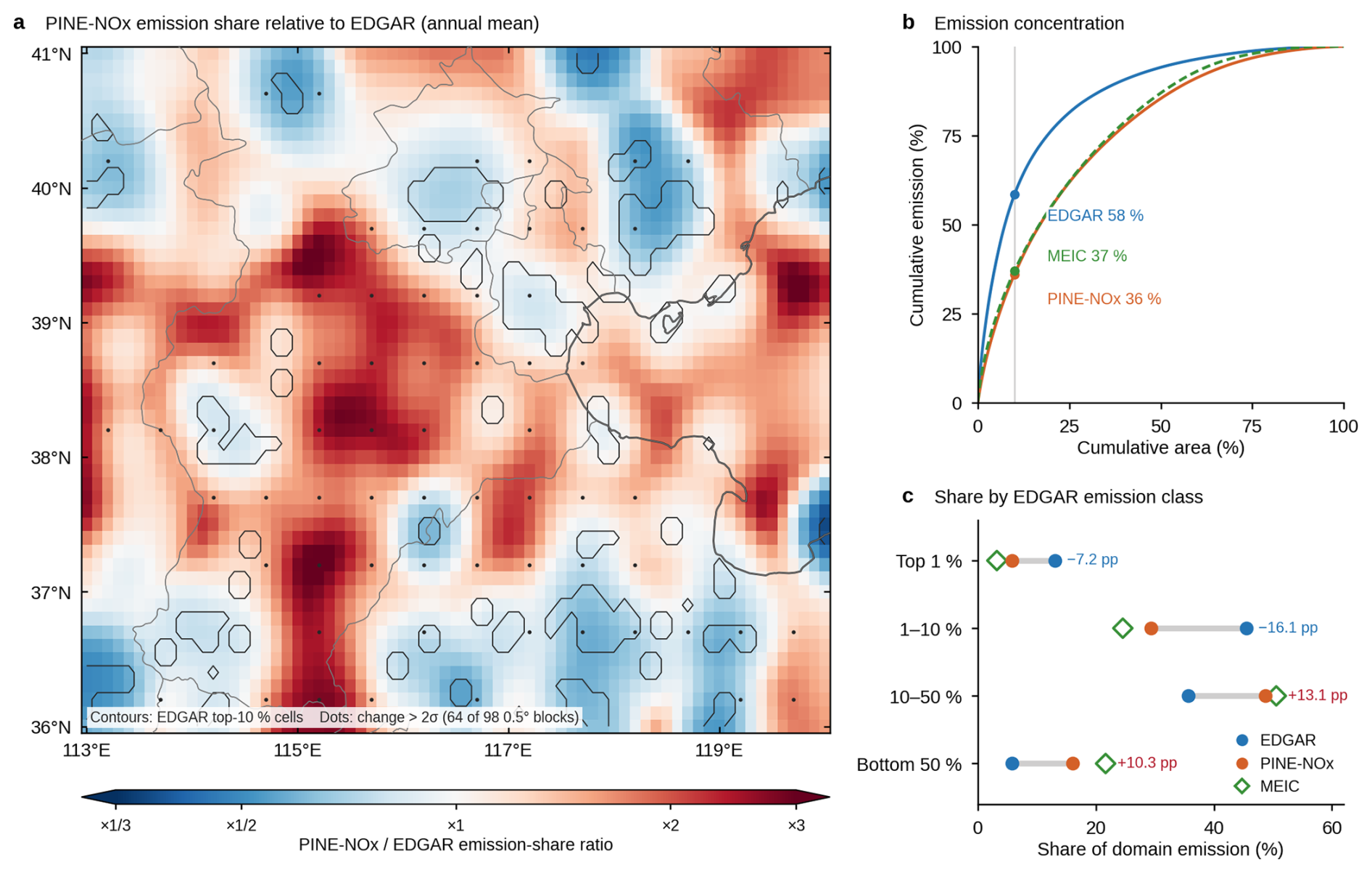
Figure 8Annual (2023) PINE-NOx emission pattern relative to the EDGAR v8.1 prior. (a) Ratio of the PINE-NOx to the EDGAR emission share in each 0.1° cell (mean of 350 daily fields; both fields smoothed with a 2-cell Gaussian kernel for display only; colour scale to ×3, 0.4 % of cells outside the scale). Black contours enclose the 10 % of cells with the largest EDGAR emissions. Dots mark the 64 of 98 0.5° blocks (blocks whose 25 cells all lie in the mask of the uncertainty budget) whose change in emission share exceeds twice its 1σ uncertainty including the prior term (Fig. 9); this uncertainty does not include the structural term estimated with the synthetic test (Sect. S1). (b) Cumulative emission against cumulative area, cells ranked by emission, for EDGAR, PINE-NOx and MEIC 2023; values give the emission share of the 10 % of the area with the highest emission of each field (cells ranked by their own emission, unlike the EDGAR ranking used in the text and in (c)). (c) Share of domain emission held by four EDGAR rank classes in EDGAR, PINE-NOx and MEIC, with the PINE-NOx minus EDGAR change in percentage points. Statistics in (b, c) use unsmoothed fields.
The uncertainty of this pattern is summarised in Fig. 9 as the 1σ of the logarithm of each cell's emission share, combining in quadrature the spread from network initialisation, regularisation weights, chemical lifetime, integration time, wind level, background estimate, retrieval noise, a ±30 % systematic error in the satellite air mass factor and the sampling of days. For the annual field this combined method-and-data term is 8.5 % at 0.5° and 15 % at 0.1° (emission-weighted). The choice of prior inventory adds a larger term (14 % and 33 %), so that the total is 17.5 % and 38 % (the combined values are emission-weighted means of the per-cell quadrature sums, so they differ from the quadrature sums of the weighted values given here). The prior term grows towards the weakly emitting cells, where the observations carry least information and where a mass-conserving inversion over China has found substantial emissions in cells with low prior values (Lu et al., 2025), and the monthly fields are 1.3–1.9 times as uncertain as the annual field (method-and-data term 11.5 %–16.5 % against 8.5 % at 0.5°), mainly because each month has fewer days. These values are lower bounds, since structural errors of the decoder are only partly represented by the variants, and the synthetic test above shows that the method alone can produce a change from EDGAR as large as the one retrieved from the observations. A narrower estimate, the spread between the four models of the season-withheld test, is shown for the daily fields in Fig. S10. Spatially, the largest inverted emissions are in three regions: the industrial corridor of central-southern Hebei (Shijiazhuang–Handan–Xingtai), the Beijing–Tianjin urban agglomeration and north-western Shandong (Jinan–Zibo). Because NO2 is carried by the wind, column maxima can lie downwind of the sources, which is why the decoder represents transport explicitly.
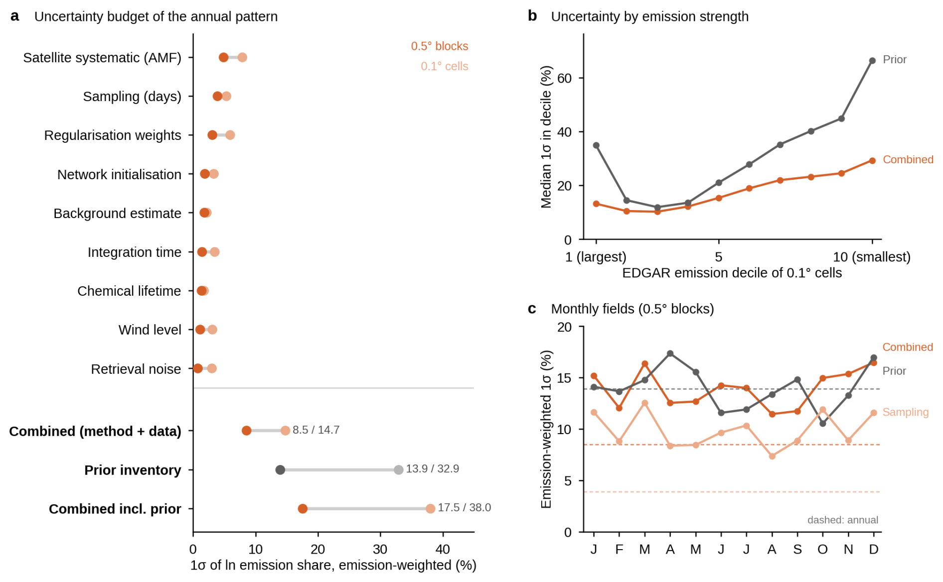
Figure 9Uncertainty of the emission pattern, expressed as 1σ of the natural logarithm of the emission share. (a) Annual budget by source, emission-weighted over 0.5° blocks (dark) and 0.1° cells (light); combined values add the sources in quadrature in each cell and are then emission-weighted, so they differ from the quadrature sum of the weighted single-source values; the prior-inventory term (EDGAR or MEIC as prior) is shown separately. (b) Median 1σ of 0.1° cells in each EDGAR emission decile, for the combined method and data terms and for the prior term. (c) Emission-weighted 1σ of the monthly fields at 0.5° for the combined term, the prior term and day sampling; dashed lines give the annual values.
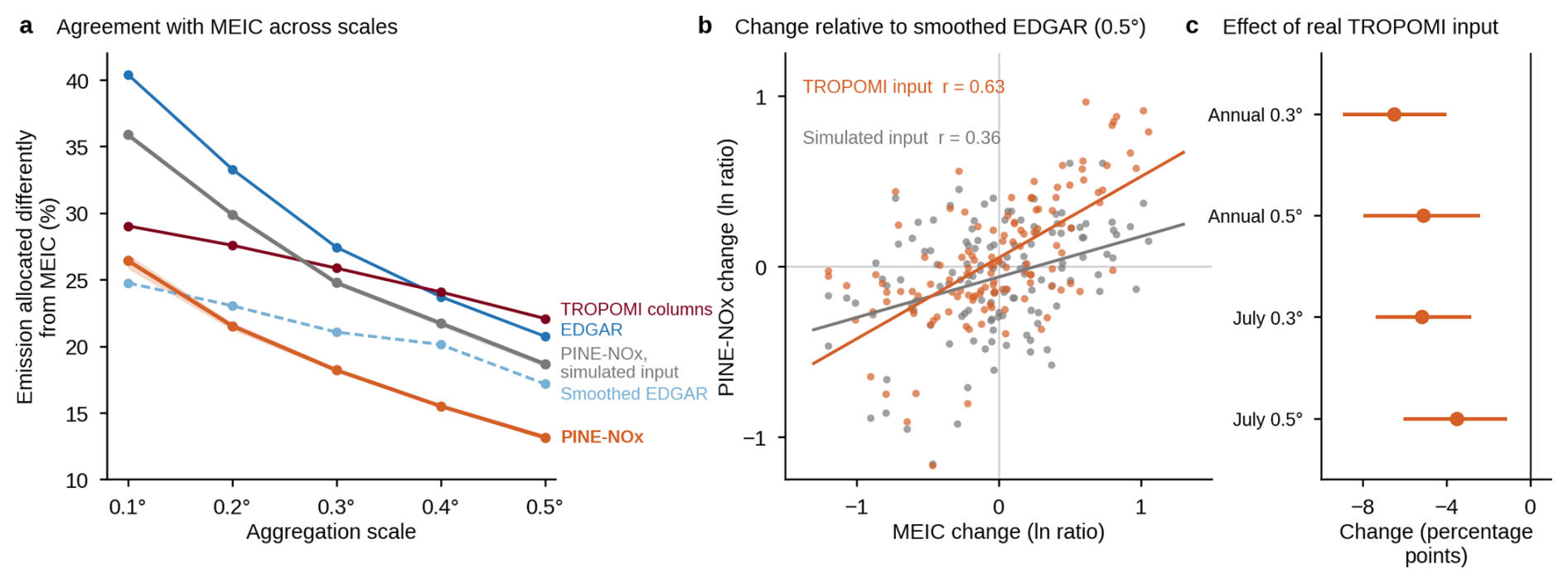
Figure 10Agreement of the annual emission patterns with MEIC 2023, which is not used by PINE-NOx. (a) Fraction of the total emission placed in different grid cells than in MEIC, (half the summed absolute difference of the emission shares, i.e. the total variation distance between the two maps; 0 % for identical allocation, 100 % for no overlap), for blocks of 0.1°−0.5° (3452–127 blocks whose 0.1° cells all have MEIC emissions). Lines show EDGAR, EDGAR smoothed with a 2-cell Gaussian kernel, the TROPOMI column pattern treated as an emission field, PINE-NOx (four network initialisations, band=range) and the decoder control, PINE-NOx with simulated input (three initialisations). The decoder control uses the identical pipeline with the TROPOMI column replaced on every day by the column that the PINE decoder computes from EDGAR (same day's wind, valid mask and background, scaled to that day's observed column level, with noise drawn from the retrieval precision); it therefore carries no TROPOMI information on the spatial pattern of emissions. (b) Change relative to smoothed EDGAR in each 0.5° block, ), for PINE-NOx with TROPOMI input and with simulated input against the corresponding MEIC change, with least-squares lines and Pearson r. (c) Paired difference in this fraction between TROPOMI input and simulated input (production network and its matching decoder control) for the annual and July fields at 0.3° and 0.5°, with 95 % block-bootstrap intervals. A stricter control with WRF-Chem columns, for July and January, is given in Table S2.
At the annual-mean scale (Fig. 8), the grid-cell log-space correlation between the PINE-NOx annual-mean emission field and the EDGAR prior is as high as r=0.937 (95 % interval 0.925–0.947 from a block bootstrap that allows for spatial autocorrelation; Fig. S13), consistent with the expectation that the prior anchors the annual-mean spatial structure. Under the design constraint that the annual total matches the prior, the departures from EDGAR are lower shares in the pollution cores (Beijing, Tianjin, Tangshan, Shijiazhuang, Handan and the Jinan–Zibo–Dezhou area) and higher shares in the weakly emitting cells and on the plain between the cores. The synthetic test produces departures of the same kind from the method alone (the departure maps of the observed and the synthetic inversions correlate across 0.1° cells with r=0.63 in July and 0.88 in January; Table S2), so their size is not attributed to the TROPOMI columns. The seasonality of the column and that of the emissions differ: under quasi-steady state the tropospheric NO2 column is approximately proportional to the product of emission flux and effective chemical lifetime (Seinfeld and Pandis, 2016), so most of the several-fold winter-summer difference in the observed column is caused by the seasonal amplification of the chemical lifetime. As a diagnostic only, we decompose the column ratio under a consistent seasonal-mean convention: the ratio of the domain's TROPOMI local column winter/summer (DJF/JJA) seasonal means is about 4.5 and the winter/summer ratio of the effective chemical lifetime is about 3.3, so the implied emission winter/summer ratio is about 1.4 but ranges from 1.1–1.8 for winter lifetimes 25 % shorter or longer (Fig. S12); this ratio is not reported as a result. The column therefore constrains the seasonal amplitude of the emissions only loosely, and the decoder, whose loss removes the domain mean every day, does not constrain it at all. The monthly totals of the product are therefore taken from the EDGAR monthly profile (winter/summer 1.09; MEIC 1.18), and the monthly fields are used only for their spatial pattern.
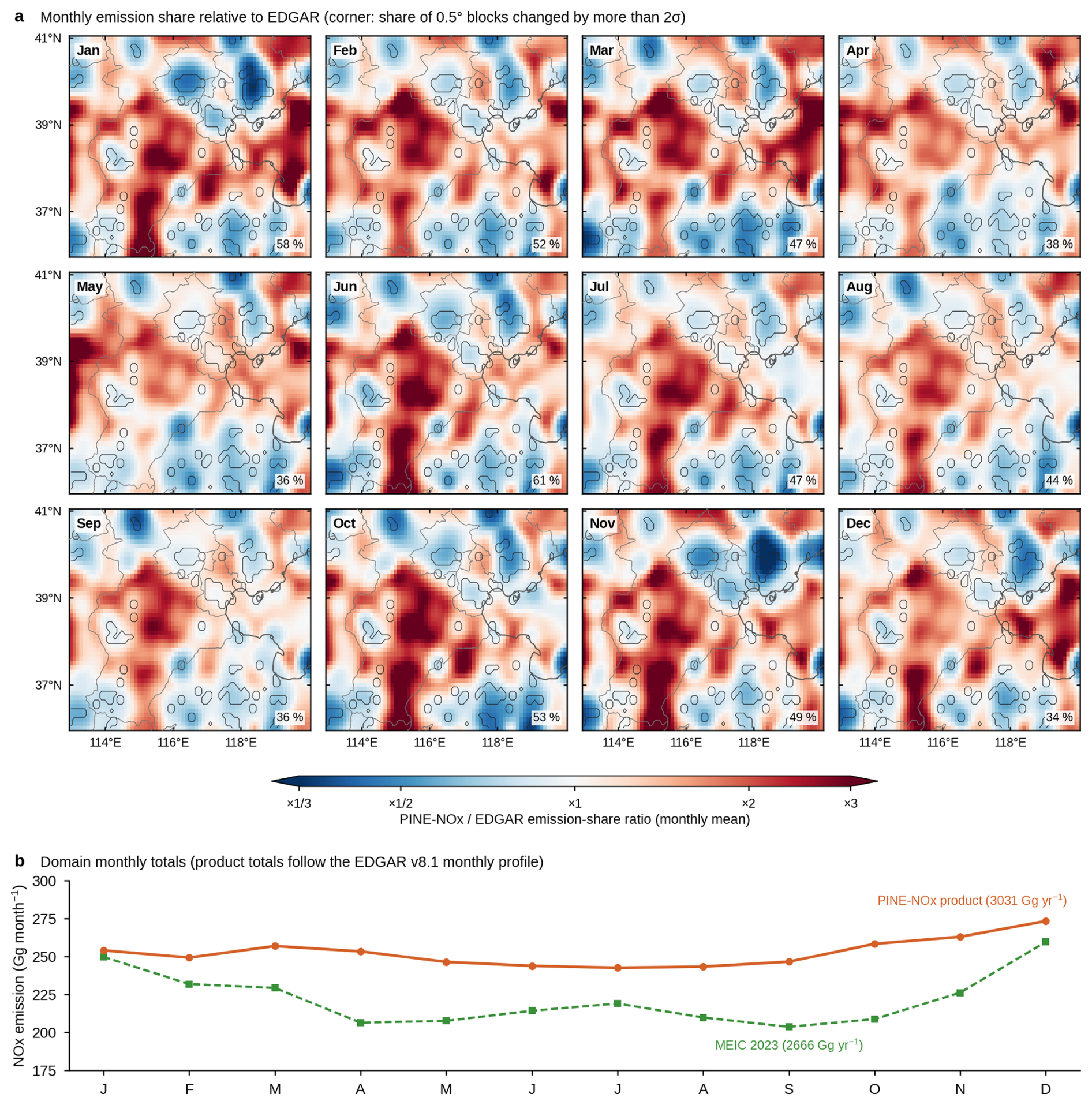
Figure 11Monthly PINE-NOx emission fields for 2023. (a) Ratio of the monthly PINE-NOx to the EDGAR emission share (display as Fig. 8a; 26–31 daily fields per month). The number in each panel is the percentage of 0.5° blocks (mask as in Fig. 8a) whose change exceeds twice the monthly 1σ uncertainty including the prior term; this uncertainty does not include the structural term of Sect. S1, so these percentages are not evidence of an observed change (Sect. 3.3). (b) Domain monthly totals. The product totals follow the EDGAR v8.1 2022 monthly profile, built from the EDGAR sector maps and China sector-specific monthly fractions, scaled to the EDGAR annual domain total (3031 Gg yr−1); MEIC 2023 monthly totals (2666 Gg yr−1) are shown for reference.
Finally, we compare the PINE-NOx pattern with MEIC, which never enters the inversion (Fig. 10). We measure the difference between two patterns as the fraction of the total emission placed in different grid cells: half the sum of the absolute differences between the emission shares of the two maps, i.e. the total variation distance between the two spatial distributions (0 % for identical allocation, 100 % for no overlap). The domain totals of EDGAR and MEIC differ by 12 % (MEIC/EDGAR=0.88), but their patterns differ more: at 0.5°, 21 % of the emissions are placed differently in EDGAR and MEIC. For PINE-NOx this fraction falls to 13 %, and the reduction holds at every aggregation scale from 0.1°–0.5°. Smoothing EDGAR with a 2-cell Gaussian kernel lowers it to 17 %; at 0.1°, however, smoothed EDGAR (25 %) is slightly closer to MEIC than PINE-NOx (26 %–27 %). The decoder control, i.e. the same inversion fed with columns that the PINE decoder simulates from EDGAR (simulated input), which contain the method's own smoothing but no observed pattern, reaches 19 % (mean of three initialisations, against 13 % for four PINE-NOx initialisations). For the annual fields of the production network and its matching decoder control, the observed TROPOMI columns lower the fraction by 5.1 percentage points at 0.5° (95 % interval 2.5–7.9) and by 6.5 points at 0.3° (4.1–8.9; Fig. 10c). This control uses the decoder of the inversion and therefore cannot contain the errors of that decoder. The synthetic test with WRF-Chem columns is a stricter control and is available for July and January (Table S2). In July, 13.5 % of the emissions are placed differently from MEIC in PINE-NOx, against 18.5 % for the inversion of the synthetic columns and 20.5 % for EDGAR. In January the values are 17.1 %, 17.8 % and 21.9 %, so no clear gain from the observations is found in that month. The test has limited power in January: columns simulated with the MEIC pattern as the true field give a retrieval only 2.2 points closer to MEIC than columns simulated from EDGAR, against 5.1 points in July (Table S2). Where MEIC departs from smoothed EDGAR, PINE-NOx departs in the same direction (annual fields: r=0.63 across 0.5° blocks, against 0.36 for the decoder control; Fig. 10b). Month by month, the PINE-NOx fields (Fig. 11) are closer to the monthly MEIC fields than both the decoder control and EDGAR in every month (Fig. 12), with the smallest gains in May and November. The month-to-month changes of the pattern, however, could not be distinguished from those produced by the method: in a test whose pass criterion was fixed before it was run, the departures of each monthly pattern from the annual pattern correlated with the corresponding MEIC departures no better for PINE-NOx than for the decoder control (pooled over months at 0.5°, to −0.05 against −0.07 to −0.06), so the monthly fields are best read as monthly realisations of the annual pattern. Because MEIC is an inventory with its own errors, these comparisons show consistency with an independent estimate, not accuracy.
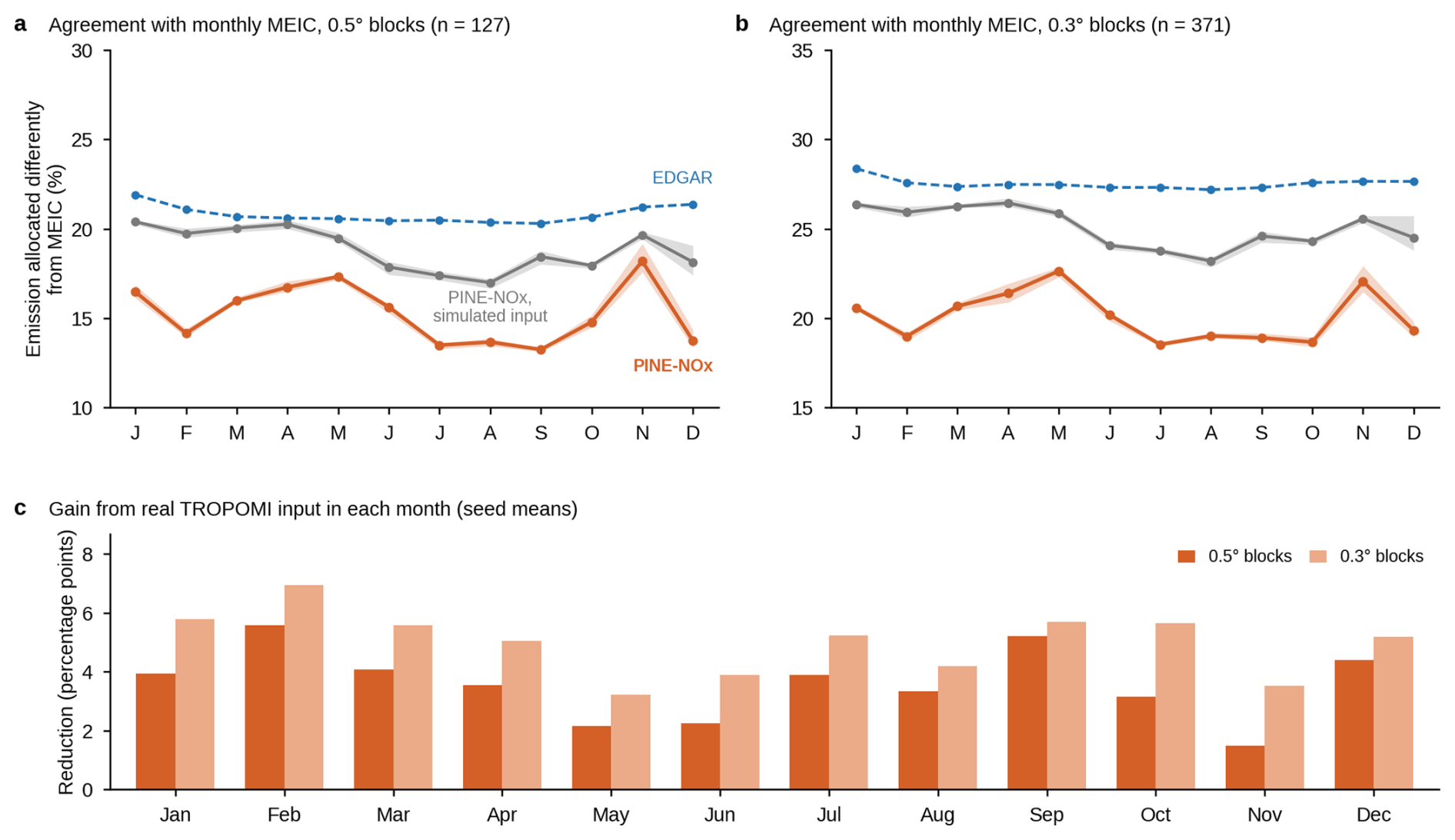
Figure 12Month-by-month agreement with the MEIC 2023 monthly fields. (a, b) Fraction of the total emission placed in different grid cells than in MEIC (as in Fig. 10a) for each month at 0.5° (127 blocks) and 0.3° (371 blocks), for EDGAR, PINE-NOx (four initialisations, band=range) and the decoder control (PINE-NOx with simulated input, three initialisations; see Fig. 10). (c) Reduction in this fraction from simulated to TROPOMI input in each month (means over initialisations), in percentage points.
4.1 Robustness of the chemical-lifetime parameterization
The monthly-mean scalar τchem parameterization is a key simplification of the forward model. The decoder renders the column by explicit integration over about 4 h in 32 steps; this window already reaches the order of the summer NOx lifetime and covers a substantial fraction of the winter lifetime; the inversion and the forward evaluation share the same fixed operator, so the conclusions are internally consistent and do not rely on a strict steady-state assumption. To systematically assess the impact of this simplification on the inversion conclusions, we conduct a progressive test at three levels: parameter sensitivity, physical-mechanism refinement and regional applicability. Over τwinter in {4, 7, 10, 15, 20} h the variation of the annual Δr does not exceed 1 % (minimum 0.533, maximum 0.537 over 80 sampled days; Fig. S2), and over τsummer in the summer Δr decreases only from 0.500–0.469, demonstrating that the reconstruction skill is insensitive to the choice of the absolute value of τchem, an insensitivity rooted in the framework's optimization target of the demeaned-VCD spatial pattern, which is insensitive to the absolute value of τchem and responds only to first order to its spatial gradient.
Drawing further on observational evidence that the NOx lifetime varies with temperature and photochemical activity (Laughner and Cohen, 2019; Stavrakou et al., 2013), we introduce a pixel-level dynamic τchem driven by the ERA5 daily surface air temperature via the Arrhenius equation (, an empirical coefficient that varies τchem by about ±20 % for a ±5 K departure from the daily domain-mean temperature; it is not a physical activation energy, since the rate coefficient of the main daytime sink, , decreases slightly with increasing temperature; Seinfeld and Pandis, 2016), whose four-season spatial coefficient of variation is about 13 %–19 % (Fig. S3); yet the improvement in Δr is only about 1 % (scalar τ: 0.535; dynamic τ: 0.542; Figs. S3 and S4). Because these tests keep the emissions fixed, we also retrained the model with eight variants of the lifetime table (scaled by 0.7 and 1.3, without its seasonal cycle, with the winter months scaled by 0.67 and 1.5, with a seasonal shape following the O(1D) photolysis frequency with and without its latitude dependence, and with a spatial lifetime pattern diagnosed from WRF-Chem); across these variants the annual emission shares change by 1.4 % at 0.5° (1σ, emission-weighted), and the share of the 10 % highest-emitting cells changes by at most 2 percentage points, small compared with its difference of about 23 percentage points from EDGAR (58.6 % against 35.2 %; Sect. 3.3), a difference of the size that the method also produces in the synthetic test. Considering both the very low parameter sensitivity and the limited improvement of the dynamic scheme, the monthly-mean scalar parameterization is justified within the accuracy framework of this paper, and the dynamic-τchem scheme is retained as an explicit direction for future improvement. In addition, a wind-zeroing advection ablation applied to the differentiable decoder shows that advective transport makes a real but secondary contribution to the forward skill: with advection switched off, the forward spatial correlation over 347 d drops from 0.871–0.778 (still far above EDGAR's 0.331), with the reduction being largest in winter (Δr≈0.12) and smallest in summer (Δr≈0.06), a seasonality consistent with the seasonal variability of wind speed and the seasonal difference in NOx lifetime, indicating that the decoder uses transport physics rather than a local rescaling of the prior.
4.2 Comparison with existing inversion methods
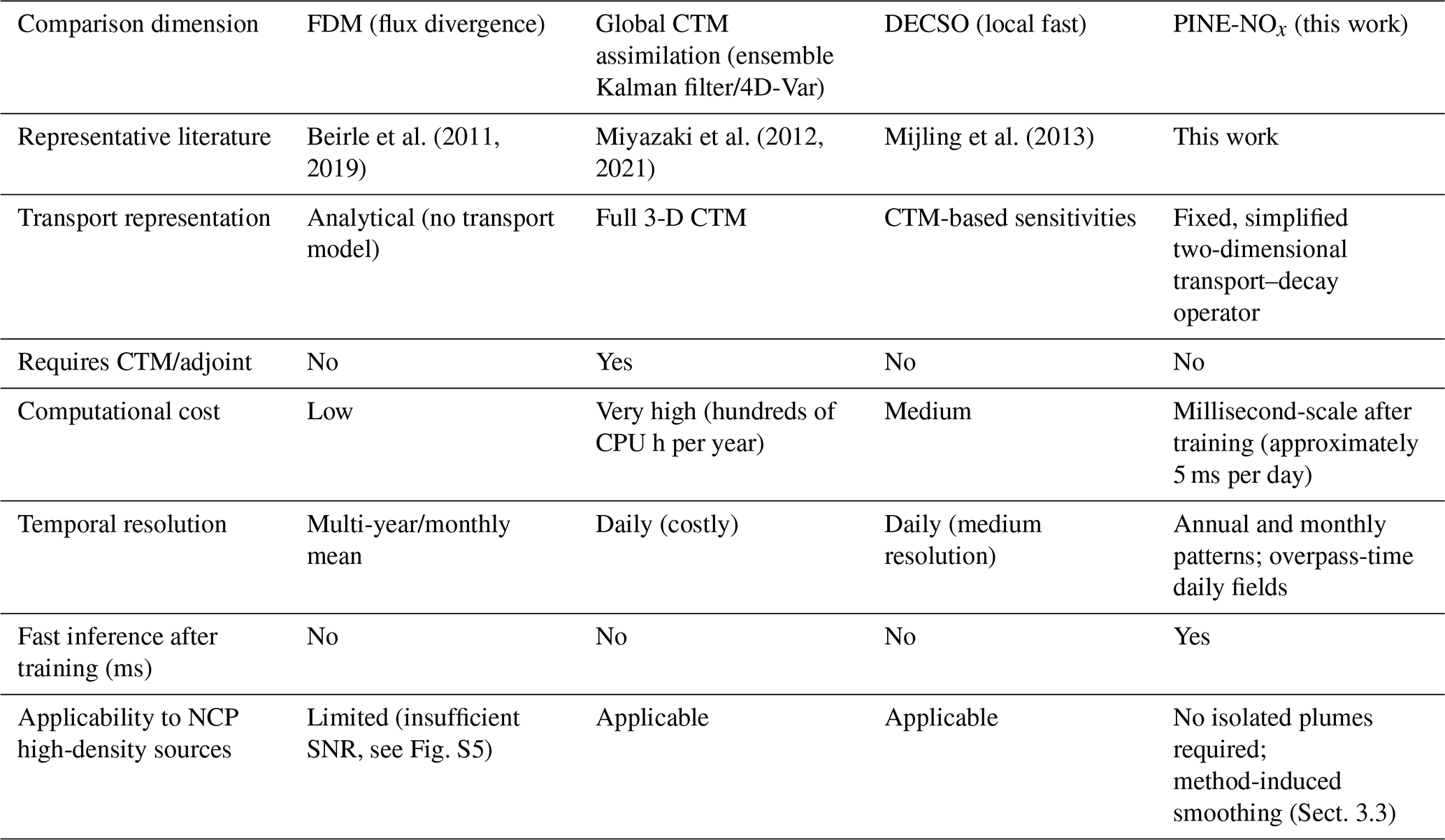
PINE-NOx combines a differentiable physical forward decoder with a neural encoder in a label-free physics-constrained autoencoder, which makes inference fast while keeping an explicit transport operator; a multidimensional comparison with representative satellite inversion methods is given in Table 3. Compared with four-dimensional variational assimilation (4D-Var), it requires no complex adjoint-model derivation, substantially lowering the engineering barrier, with single-day inference at the millisecond scale, at the price of a much simpler transport and chemistry description; compared with the FDM, it does not require isolated plumes, uniform wind or a clean background, conditions that are not met over the NCP (Fig. S5), although the method itself smooths the emission pattern (Sect. 3.3); compared with methods supervised by existing inversion products, PINE-NOx relies on no emission label, and emissions are inverted directly as a physical latent variable, avoiding the circularity of training on inventory-derived labels; it still depends on a prior, whose influence is quantified in Sect. 3.3. A physics-informed neural network that embeds the mass-continuity equation in its training has recently been applied to TROPOMI columns over the Yangtze River Delta (He et al., 2026); in PINE-NOx the transport–chemistry operator is not learned but enters as a fixed decoder.
Table 3Comparison of PINE-NOx with representative satellite NOx emission-inversion methods.
4.3 Limitations and future directions
The current framework has several limitations worth stating explicitly. First, the forward evaluation uses the demeaned log-space spatial correlation as its metric, characterizing spatial-pattern skill; the network targets reconstruction of the observed pattern and does not constrain absolute magnitude, so the RMSE of the daily absolute magnitude is not its optimization objective, and conclusions should be interpreted primarily in terms of spatial pattern. To provide an external reference, we carried out a WRF-Chem three-dimensional forward-simulation consistency experiment (see Sect. 3.2 and Fig. 7). We emphasize that the absolute magnitude of the inversion is not determined independently by the observations: the rendering loss is demeaned log, and the domain annual total is locked to EDGAR by design, so the agreement of the annual total with EDGAR is a design constraint rather than an independent validation; what the observations constrain is the spatial pattern. The seasonal amplitude and the day-to-day variation of the domain total are not constrained either, and the month-to-month changes of the pattern could not be separated from those produced by the method itself (Sect. 3.3). The pattern depends on the prior inventory, and this is the largest term of the uncertainty budget, especially in weakly emitting cells. A synthetic test with known emissions (Sects. 3.3 and S1) shows that the method by itself moves emission share out of the urban–industrial cores by about as much as the inversion of the observed columns does. Of the possible causes (the simplified decoder, the smoother 27 km model columns and the use of networks trained on TROPOMI on simulated columns), the two-dimensional decoder is the most likely one, because it departs most from the three-dimensional atmosphere. The size of the change from EDGAR is therefore not reported as a result. The comparisons with independent data leave the evidence uneven: the PINE-NOx pattern is closer to MEIC (clearly in July and not in January when compared with the synthetic test), but in one month of WRF-Chem simulation it does not improve agreement with surface stations. Both MEIC and the station comparison have their own errors, and a test against facility-level or flux observations would be needed to settle which allocation is closer to the truth. Second, the monthly-mean scalar chemical lifetime is a simplification, whose sensitivity is examined in Sect. 4.1 and Figs. S2–S4. In addition, advection uses the ERA5 10 m daytime-mean wind to approximate column-mean transport, which may underestimate transport aloft; however, the advection ablation shows this to be a secondary contribution (Δr≈0.09; see Sect. 4.1), and across retrainings with the 10 m, the 100 m and the boundary-layer mean wind the annual emission shares differ by about 1 % at 0.5° and 3 % at 0.1° (1σ, emission-weighted; Fig. 9). Finally, the framework currently targets a single species (NOx) and region (the NCP); extending it to other pollutants (e.g. SO2, NH3; for SO2, for instance, space-based point sources have been catalogued by Fioletov et al., 2016) and regions, and fusing multi-source satellite and ground-based flux observations to constrain the absolute magnitude independently, is a worthwhile future direction.
The prior inventory also limits what can be learned in weakly emitting cells. The cells that together hold the lowest 10 % of the EDGAR total cover more than half of the domain (about 2200 of 3621 cells). In these cells the column produced by a cell's own emissions is small compared with the precision of a single TROPOMI overpass, and most of the local column is transported in from elsewhere. The satellite therefore cannot tell, cell by cell, whether a low prior value reflects small emissions or a misallocation in the inventory, and the retrieved emissions there are highly uncertain and largely set by the prior; the prior term of the uncertainty budget is largest in these cells (Fig. 9b). MEIC places 32 % of its domain total in these cells, PINE-NOx 25 % and EDGAR 10 %. The synthetic test, however, raises the share of the weakly emitting cells by a similar amount when the true emissions equal EDGAR (Sect. 3.3), so the inversion cannot confirm whether emissions are missing from EDGAR in these regions. Such emissions may still matter. During the Spring Festival (Chinese New Year), when many people move from the cities to rural homes, NO2 falls strongly in the cities (Li et al., 2021), whereas household energy use and air-pollution exposure increase in rural areas (Hua et al., 2021; Shen et al., 2021); a pattern anchored to a static prior inventory cannot capture such a shift.
The form of the network output sets a further limit. The emissions are the prior multiplied by exp (δ), with δ bounded to ±3 (Sect. 2.3), so a cell can receive at most 20 times its prior value and a cell without prior emission stays at zero. PINE-NOx therefore does not address the sources that satellite inversions have found where inventories have no or very small emissions (McLinden et al., 2016; Qin et al., 2023; Liu et al., 2024; Lu et al., 2025).
In the uncertainty budget the retrieval errors enter as random noise from the pixel precision of the TROPOMI product and as a ±30 % systematic air-mass-factor error (Sect. 3.3), and the synthetic test adds random noise with the same statistics everywhere (Sect. S1). Over the North China Plain the errors of tropospheric NO2 columns are neither uniform nor linear. The air mass factor depends on the amount of aerosol and its height relative to the NO2 layer, on clouds, on the surface albedo and on the a priori profile, and these dependences change from cell to cell and from day to day (Leitão et al., 2010; Lorente et al., 2017; Liu et al., 2020). Over polluted areas the columns are biased low by amounts that grow with the pollution level (Verhoelst et al., 2021; van Geffen et al., 2022). Clouds and heavy aerosol also decide which pixels pass the quality screening, so the edges of the valid data move with the weather and the remaining days are not a random sample. Where the plumes of neighbouring sources overlap, such errors change the shape of the column field and can move signal from one source to the next, which the decoder then assigns to the wrong cells (Beirle et al., 2019, 2021). These effects are not represented in the inversion, so the allocation between adjacent cells, particularly in the aerosol-rich winter months, is less certain than Fig. 9 indicates.
A further intrinsic limitation concerns temporal sampling. Sentinel-5P/TROPOMI provides only a single overpass per day (about 13:30 local solar time), so each retrieval is an instantaneous snapshot of the NO2 column at a fixed hour, whereas the quantity we infer is an effective emission at overpass time. It should not be read as a 24 h mean emission rate: the diurnal cycle of emissions and of the chemical lifetime is not directly observed, and is instead absorbed into the effective quantities through the demeaned rendering loss and the monthly-mean lifetime parameterization. A natural way forward is to fuse multiple, temporally complementary observational constraints: continuous ground-based networks provide near-surface, high-frequency anchoring, while the new generation of geostationary spectrometers (GEMS over East Asia, together with TEMPO and Sentinel-4) delivers hourly daytime columns that, combined with polar-orbiting sensors such as OMI and TROPOMI, would substantially densify the temporal and spatial sampling. Embedding such multi-source constraints within the same differentiable, physics-constrained framework is a promising route to a more accurate inventory that explicitly resolves the intraday dynamics of NOx emissions, which we leave for future work.
4.4 The emission pattern in the context of other satellite inversions
Moving emission from strong sources into their surroundings is a known behaviour of satellite inversions. When the observations do not carry enough information to resolve every grid cell, the solution is smoothed towards the prior or across neighbouring cells, whereas a coarser state vector imposes the prior pattern instead (Turner and Jacob, 2015). Mass-balance inversions of NO2 columns spread local emission changes over their surroundings through NOx transport, which adjoint inversions resolve better (Cooper et al., 2017). The finite footprint of the satellite pixels smooths the observed field further when it is averaged onto a grid (Sun et al., 2018). The synthetic test of Sect. 3.3 measures this effect for PINE-NOx, and its size equals that of the departure from EDGAR.
For NOx, spatial attribution is complicated further by non-linear chemistry. The NOx lifetime depends on the NOx concentration through its effect on OH, so it differs between the centre of an urban plume and its edges and between seasons (Valin et al., 2013; Laughner and Cohen, 2019); over eastern China the winter lifetime is several times the summer one (Shah et al., 2020). Model columns computed at a resolution coarser than the plumes are biased low over large sources and high over small ones (Valin et al., 2011). The PINE-NOx decoder uses a first-order loss with a monthly lifetime and does not represent this concentration dependence. Part of the difference between the observed and the simulated column patterns that the inversion assigns to emissions may therefore reflect differences in the effective lifetime between the cores and their surroundings.
Other species show how transport and retrieval interference separate satellite signals from their source grids. For CO, which is long-lived, top-down regional source estimates change by tens of percent with the transport model used (Arellano and Hess, 2006; Jiang et al., 2011), transport across provincial boundaries contributes substantially to the columns over Chinese source regions (Li et al., 2025), and plumes lofted from fires are observed far from their sources (Lin et al., 2020). For aerosols, source inversions depend on the modelled transport and removal (Dubovik et al., 2008; Cohen and Wang, 2014), and the aerosols also alter the trace-gas retrievals themselves (Leitão et al., 2010; Liu et al., 2019). NOx lives for hours in summer and for about a day in winter (Beirle et al., 2011; Shah et al., 2020), so its columns stay closer to the source pattern than those of CO, which is what makes a two-dimensional decoder with first-order loss workable at 0.1°; the same short lifetime makes the result sensitive to the chemistry and to retrieval errors near the sources. Within these limits, PINE-NOx describes how the observed column pattern departs from the pattern expected from a prior inventory under simplified transport and chemistry, and whether these departures move the pattern towards an independent inventory. Absolute emissions, the split of emissions within overlapping plumes, the concentration dependence of the NOx lifetime and sources absent from the prior are outside its reach.
We have proposed the PINE-NOx emission-inversion framework, which fuses a differentiable physical forward decoder and a neural encoder end-to-end into a label-free physics-constrained autoencoder, and applied it to the spatial pattern of NOx emissions over the North China Plain from TROPOMI, systematically comparing convolutional, spectral-operator and spectral-fusion encoder backbones. The reconstruction test shows that, on the 54 validation days, which were not used to fit the weights but were used to select the checkpoint, the forward VCD driven by the PINE-NOx-inverted emissions improves its spatial correlation with TROPOMI from r=0.332 to r=0.856; over all 347 d the values are 0.331 and 0.871, with improvement in all four seasons (winter (DJF) 0.871, spring (MAM) 0.869, summer (JJA) 0.860, autumn (SON) 0.883) and little difference between encoder backbones. This is a reconstruction of the observations, not a validation of the emissions. The annual total is held at EDGAR, and the observations adjust the daily relative spatial pattern around the prior, which still governs the magnitude and the large-scale structure of the emission field (annual r=0.937 with EDGAR). The PINE-NOx field places less of the emissions in the urban–industrial cores than EDGAR, but a synthetic test with known emissions shows that a decrease of this size also arises from the method itself; this shift is primarily a structural artefact, most likely of the two-dimensional decoder, and not an independently observed signal. Emissions missing from EDGAR in weakly emitting cells, and sources where the prior has none, cannot be identified with this approach. The pattern is closer to the MEIC inventory, which the inversion never uses. Compared with the synthetic test, the observed columns bring the July pattern closer to MEIC (13.5 % of the emissions placed in different 0.5° cells than in MEIC, against 18.5 % in the test and 20.5 % for EDGAR), whereas no clear gain is found in January. The test is limited to two months and a 27 km model and does not simulate retrieval biases such as air-mass-factor errors. In a WRF-Chem consistency check the new pattern brings the simulated columns closer to TROPOMI but does not improve the agreement with surface stations, so the allocation it proposes still needs an independent test. The same pattern is provided as annual and monthly fields with uncertainty estimates. With label-free training and millisecond inference, PINE-NOx offers a practical approach to atmospheric emission inversion, provided that its departures from the prior are checked with a synthetic test of this kind.
All datasets used in this study are publicly available. Sentinel-5P/TROPOMI tropospheric NO2 columns are available from the Copernicus Sentinel-5P Data Hub (https://dataspace.copernicus.eu, last access: 13 November 2026). ERA5 reanalysis fields are available from the Copernicus Climate Data Store (https://cds.climate.copernicus.eu, last access: 13 November 2026). The EDGAR v8.1 NOx emission inventory is distributed by the European Commission Joint Research Centre (https://edgar.jrc.ec.europa.eu, last access: 13 November 2026). The MEIC anthropogenic emission inventory is available from the MEIC team, Tsinghua University (http://meicmodel.org.cn, last access: 13 November 2026). Hourly surface NO2 observations are from the China National Environmental Monitoring Centre (CNEMC, https://www.cnemc.cn, last access: 13 November 2026). For the WRF-Chem consistency check, CAMS EAC4 chemical fields are available from the Copernicus Atmosphere Monitoring Service (https://ads.atmosphere.copernicus.eu, last access: 13 November 2026) and NCEP GDAS/FNL meteorological data from the NCAR Research Data Archive (https://rda.ucar.edu, last access: 13 November 2026). Coal-fired power-plant locations and capacities shown in Figs. 1 and S5 are from the WRI Global Power Plant Database, which builds on the Global Coal Plant Tracker. WRF-Chem is an open-source community model (https://www2.mmm.ucar.edu/wrf/users/, last access: 13 November 2026).
The PINE-NOx emission fields generated in this study (annual, monthly and overpass-time daily, 0.1°, 2023), the trained network weights with the code needed to compute the emission fields from the input data, the gridded input data, and the data and scripts used to produce the figures are available at Zenodo (https://doi.org/10.5281/zenodo.20725610, Wang et al., 2026). The departure of these fields from EDGAR is of the size that the method produces on its own in a synthetic test (Sects. 3.3 and S1).
The supplement related to this article is available online at https://doi.org/10.5194/acp-26-16125-2026-supplement.
YW and YP conceived and designed the study. YW developed the PINE-NOx framework and the differentiable physical decoder, implemented the software, performed the inversion experiments and the WRF-Chem simulations, carried out the formal analysis and visualization, and wrote the original draft. YP provided supervision and computational resources, guided the methodology and interpretation of results, and revised the manuscript. DL provided scientific guidance and advice throughout the study, contributed to the interpretation of the results, and reviewed and edited the manuscript. All authors have read and approved the final version.
The contact author has declared that none of the authors has any competing interests.
Publisher's note: Copernicus Publications remains neutral with regard to jurisdictional claims made in the text, published maps, institutional affiliations, or any other geographical representation in this paper. The authors bear the ultimate responsibility for providing appropriate place names. Views expressed in the text are those of the authors and do not necessarily reflect the views of the publisher.
Yinan Wang gratefully acknowledges the support of Phase II of the Chinese Meridian Project.
This research has been supported by the National Natural Science Foundation of China (grant no. 42293321).
This paper was edited by Jason Cohen and reviewed by two anonymous referees.
Arellano, A. F. and Hess, P. G.: Sensitivity of top-down estimates of CO sources to GCTM transport, Geophys. Res. Lett., 33, L21807, https://doi.org/10.1029/2006GL027371, 2006.
Beirle, S., Boersma, K. F., Platt, U., Lawrence, M. G., and Wagner, T.: Megacity Emissions and Lifetimes of Nitrogen Oxides Probed from Space, Science, 333, 1737–1739, https://doi.org/10.1126/science.1207824, 2011.
Beirle, S., Borger, C., Dörner, S., Li, A., Hu, Z., Liu, F., Wang, Y., and Wagner, T.: Pinpointing nitrogen oxide emissions from space, Sci. Adv., 5, eaax9800, https://doi.org/10.1126/sciadv.aax9800, 2019.
Beirle, S., Borger, C., Dörner, S., Eskes, H., Kumar, V., de Laat, A., and Wagner, T.: Catalog of NOx emissions from point sources as derived from the divergence of the NO2 flux for TROPOMI, Earth Syst. Sci. Data, 13, 2995–3012, https://doi.org/10.5194/essd-13-2995-2021, 2021.
Boersma, K. F., Eskes, H. J., and Brinksma, E. J.: Error analysis for tropospheric NO2 retrieval from space, J. Geophys. Res., 109, https://doi.org/10.1029/2003JD003962, 2004.
Boersma, K. F., Eskes, H. J., Richter, A., De Smedt, I., Lorente, A., Beirle, S., van Geffen, J. H. G. M., Zara, M., Peters, E., Van Roozendael, M., Wagner, T., Maasakkers, J. D., van der A, R. J., Nightingale, J., De Rudder, A., Irie, H., Pinardi, G., Lambert, J.-C., and Compernolle, S. C.: Improving algorithms and uncertainty estimates for satellite NO2 retrievals: results from the quality assurance for the essential climate variables (QA4ECV) project, Atmos. Meas. Tech., 11, 6651–6678, https://doi.org/10.5194/amt-11-6651-2018, 2018.
Chen, L., Cai, Z., Sun, K., Liu, Y., Yang, D., Li, M., and Zhu, L.: Deriving regional and point source nitrogen oxides emissions in China from TROPOMI using the directional derivative approach with nonlinear chemical lifetime fitting, Earth Syst. Sci. Data, 18, 2749–2767, https://doi.org/10.5194/essd-18-2749-2026, 2026.
Cohen, J. B. and Wang, C.: Estimating global black carbon emissions using a top-down Kalman Filter approach, J. Geophys. Res.-Atmos., 119, 307–323, https://doi.org/10.1002/2013JD019912, 2014.
Cooper, M., Martin, R. V., Padmanabhan, A., and Henze, D. K.: Comparing mass balance and adjoint methods for inverse modeling of nitrogen dioxide columns for global nitrogen oxide emissions, J. Geophys. Res., 122, 4718–4734, https://doi.org/10.1002/2016JD025985, 2017.
Cranmer, K., Brehmer, J., and Louppe, G.: The frontier of simulation-based inference, P. Natl. Acad. Sci. USA, 117, 30055–30062, https://doi.org/10.1073/pnas.1912789117, 2020.
Crippa, M., Guizzardi, D., Pagani, F., Banja, M., Muntean, M., Schaaf, E., Becker, W., Monforti-Ferrario, F., Quadrelli, R., Risquez Martin, A., Grassi, G., Rossi, S., Brandao De Melo, J., Jacome Felix Oom, D., Branco, A., San-Miguel, J., and Vignati, E.: EDGAR v8.1 Global Air Pollutant Emissions, European Commission, Joint Research Centre [data set], https://doi.org/10.2905/JRC.E1ZGQER, 2026.
de Foy, B., Lu, Z., Streets, D. G., Lamsal, L. N., and Duncan, B. N.: Estimates of power plant NOx emissions and lifetimes from OMI NO2 satellite retrievals, Atmos. Environ., 116, 1–11, https://doi.org/10.1016/j.atmosenv.2015.05.056, 2015.
Dubovik, O., Lapyonok, T., Kaufman, Y. J., Chin, M., Ginoux, P., Kahn, R. A., and Sinyuk, A.: Retrieving global aerosol sources from satellites using inverse modeling, Atmos. Chem. Phys., 8, 209–250, https://doi.org/10.5194/acp-8-209-2008, 2008.
Fioletov, V. E., McLinden, C. A., Krotkov, N., Li, C., Joiner, J., Theys, N., Carn, S., and Moran, M. D.: A global catalogue of large SO2 sources and emissions derived from the Ozone Monitoring Instrument, Atmos. Chem. Phys., 16, 11497–11519, https://doi.org/10.5194/acp-16-11497-2016, 2016.
Geng, G., Zheng, Y., Zhang, Q., Xue, T., Zhao, H., Tong, D., Zheng, B., Li, M., Liu, F., Hong, C., He, K., and Davis, S. J.: Drivers of PM2.5 air pollution deaths in China 2002–2017, Nat. Geosci., 14, 645–650, https://doi.org/10.1038/s41561-021-00792-3, 2021.
Goldberg, D. L., Lu, Z., Streets, D. G., de Foy, B., Griffin, D., McLinden, C. A., Lamsal, L. N., Krotkov, N. A., and Eskes, H.: Enhanced Capabilities of TROPOMI NO2: Estimating NOx from North American Cities and Power Plants, Environ. Sci. Technol., 53, 12594–12601, https://doi.org/10.1021/acs.est.9b04488, 2019.
Goldberg, D. L., Anenberg, S. C., Griffin, D., McLinden, C. A., Lu, Z., and Streets, D. G.: Disentangling the Impact of the COVID-19 Lockdowns on Urban NO 2 From Natural Variability, Geophys. Res. Lett., 47, e2020GL089269, https://doi.org/10.1029/2020GL089269, 2020.
Goldberg, D. L., Harkey, M., de Foy, B., Judd, L., Johnson, J., Yarwood, G., and Holloway, T.: Evaluating NOx emissions and their effect on O3 production in Texas using TROPOMI NO2 and HCHO, Atmos. Chem. Phys., 22, 10875–10900, https://doi.org/10.5194/acp-22-10875-2022, 2022.
He, Q., Qin, K., Gao, H., Wong, M. S., and Cohen, J. B.: Revealing spatiotemporal NOx emission dynamics in the Yangtze River Delta using physics-informed neural networks and TROPOMI observations, Environ. Res., 310, 125952, https://doi.org/10.1016/j.envres.2026.125952, 2026.
Hersbach, H., Bell, B., Berrisford, P., Hirahara, S., Horányi, A., Muñoz-Sabater, J., Nicolas, J., Peubey, C., Radu, R., Schepers, D., Simmons, A., Soci, C., Abdalla, S., Abellan, X., Balsamo, G., Bechtold, P., Biavati, G., Bidlot, J., Bonavita, M., Chiara, G. de, Dahlgren, P., Dee, D., Diamantakis, M., Dragani, R., Flemming, J., Forbes, R., Fuentes, M., Geer, A., Haimberger, L., Healy, S., Hogan, R. J., Hólm, E., Janisková, M., Keeley, S., Laloyaux, P., Lopez, P., Lupu, C., Radnoti, G., Rosnay, P. de, Rozum, I., Vamborg, F., Villaume, S., and Thépaut, J.-N.: The ERA5 global reanalysis, Q. J. Roy. Meteor. Soc., 146, 1999–2049, https://doi.org/10.1002/qj.3803, 2020.
Hua, J., Zhang, Y., de Foy, B., Mei, X., Shang, J., and Feng, C.: Competing PM2.5 and NO2 holiday effects in the Beijing area vary locally due to differences in residential coal burning and traffic patterns, Sci. Total Environ., 750, 141575, https://doi.org/10.1016/j.scitotenv.2020.141575, 2021.
Jiang, Z., Jones, D. B. A., Kopacz, M., Liu, J., Henze, D. K., and Heald, C.: Quantifying the impact of model errors on top-down estimates of carbon monoxide emissions using satellite observations, J. Geophys. Res., 116, D15306, https://doi.org/10.1029/2010JD015282, 2011.
Jin, X. and Holloway, T.: Spatial and temporal variability of ozone sensitivity over China observed from the Ozone Monitoring Instrument, J. Geophys. Res., 120, 7229–7246, https://doi.org/10.1002/2015JD023250, 2015.
Karniadakis, G. E., Kevrekidis, I. G., Lu, L., Perdikaris, P., Wang, S., and Yang, L.: Physics-informed machine learning, Nat. Rev. Phys., 3, 422–440, https://doi.org/10.1038/s42254-021-00314-5, 2021.
Kingma, D. P. and Ba, J.: Adam: A Method for Stochastic Optimization, in: Proceedings of the International Conference on Learning Representations (ICLR), San Diego, CA, USA, 7–9 May 2015, https://doi.org/10.48550/arXiv.1412.6980, 2015.
Kong, H., Lin, J., Zhang, R., Liu, M., Weng, H., Ni, R., Chen, L., Wang, J., Yan, Y., and Zhang, Q.: High-resolution (0.05°×0.05°) NOx emissions in the Yangtze River Delta inferred from OMI, Atmos. Chem. Phys., 19, 12835–12856, https://doi.org/10.5194/acp-19-12835-2019, 2019.
Laughner, J. L. and Cohen, R. C.: Direct observation of changing NOx lifetime in North American cities, Science, 366, 723–727, https://doi.org/10.1126/science.aax6832, 2019.
Leitão, J., Richter, A., Vrekoussis, M., Kokhanovsky, A., Zhang, Q. J., Beekmann, M., and Burrows, J. P.: On the improvement of NO2 satellite retrievals – aerosol impact on the airmass factors, Atmos. Meas. Tech., 3, 475–493, https://doi.org/10.5194/amt-3-475-2010, 2010.
Li, D., Wu, Q., Wang, H., Xiao, H., Xu, Q., Wang, L., Feng, J., Yang, X., Cheng, H., Wang, L., and Sun, Y.: The Spring Festival Effect: The change in NO2 column concentration in China caused by the migration of human activities, Atmos. Pollut. Res., 12, 101232, https://doi.org/10.1016/j.apr.2021.101232, 2021.
Li, M., Zhang, Q., Kurokawa, J.-I., Woo, J.-H., He, K., Lu, Z., Ohara, T., Song, Y., Streets, D. G., Carmichael, G. R., Cheng, Y., Hong, C., Huo, H., Jiang, X., Kang, S., Liu, F., Su, H., and Zheng, B.: MIX: a mosaic Asian anthropogenic emission inventory under the international collaboration framework of the MICS-Asia and HTAP, Atmos. Chem. Phys., 17, 935–963, https://doi.org/10.5194/acp-17-935-2017, 2017.
Li, X., Cohen, J. B., Tiwari, P., Wu, L., Wang, S., He, Q., Yang, H., and Qin, K.: Space-based inversion reveals underestimated carbon monoxide emissions over Shanxi, Commun. Earth Environ., 6, 357, https://doi.org/10.1038/s43247-025-02301-5, 2025.
Li, Z., Kovachki, N., Azizzadenesheli, K., Liu, B., Bhattacharya, K., Stuart, A., and Anandkumar, A.: Fourier Neural Operator for Parametric Partial Differential Equations, arXiv [preprint], https://doi.org/10.48550/arXiv.2010.08895, 2020.
Lin, C., Cohen, J. B., Wang, S., Lan, R., and Deng, W.: A new perspective on the spatial, temporal, and vertical distribution of biomass burning: quantifying a significant increase in CO emissions, Environ. Res. Lett., 15, 104091, https://doi.org/10.1088/1748-9326/abaa7a, 2020.
Liu, F., Beirle, S., Zhang, Q., Dörner, S., He, K., and Wagner, T.: NOx lifetimes and emissions of cities and power plants in polluted background estimated by satellite observations, Atmos. Chem. Phys., 16, 5283–5298, https://doi.org/10.5194/acp-16-5283-2016, 2016.
Liu, J., Cohen, J. B., He, Q., Tiwari, P., and Qin, K.: Accounting for NOx emissions from biomass burning and urbanization doubles existing inventories over South, Southeast and East Asia, Commun. Earth Environ., 5, 255, https://doi.org/10.1038/s43247-024-01424-5, 2024.
Liu, M., Lin, J., Boersma, K. F., Pinardi, G., Wang, Y., Chimot, J., Wagner, T., Xie, P., Eskes, H., Van Roozendael, M., Hendrick, F., Wang, P., Wang, T., Yan, Y., Chen, L., and Ni, R.: Improved aerosol correction for OMI tropospheric NO2 retrieval over East Asia: constraint from CALIOP aerosol vertical profile, Atmos. Meas. Tech., 12, 1–21, https://doi.org/10.5194/amt-12-1-2019, 2019.
Liu, M., Lin, J., Kong, H., Boersma, K. F., Eskes, H., Kanaya, Y., He, Q., Tian, X., Qin, K., Xie, P., Spurr, R., Ni, R., Yan, Y., Weng, H., and Wang, J.: A new TROPOMI product for tropospheric NO2 columns over East Asia with explicit aerosol corrections, Atmos. Meas. Tech., 13, 4247–4259, https://doi.org/10.5194/amt-13-4247-2020, 2020.
Lorente, A., Folkert Boersma, K., Yu, H., Dörner, S., Hilboll, A., Richter, A., Liu, M., Lamsal, L. N., Barkley, M., De Smedt, I., Van Roozendael, M., Wang, Y., Wagner, T., Beirle, S., Lin, J.-T., Krotkov, N., Stammes, P., Wang, P., Eskes, H. J., and Krol, M.: Structural uncertainty in air mass factor calculation for NO2 and HCHO satellite retrievals, Atmos. Meas. Tech., 10, 759–782, https://doi.org/10.5194/amt-10-759-2017, 2017.
Lu, L., Cohen, J. B., Qin, K., Li, X., and He, Q.: Identifying missing sources and reducing NOx emissions uncertainty over China using daily satellite data and a mass-conserving method, Atmos. Chem. Phys., 25, 2291–2309, https://doi.org/10.5194/acp-25-2291-2025, 2025.
Lu, X., Zhang, L., Chen, Y., Zhou, M., Zheng, B., Li, K., Liu, Y., Lin, J., Fu, T.-M., and Zhang, Q.: Exploring 2016–2017 surface ozone pollution over China: source contributions and meteorological influences, Atmos. Chem. Phys., 19, 8339–8361, https://doi.org/10.5194/acp-19-8339-2019, 2019.
Martin, R. V., Jacob, D. J., Chance, K., Kurosu, T. P., Palmer, P. I., and Evans, M. J.: Global inventory of nitrogen oxide emissions constrained by space-based observations of NO2 columns, J. Geophys. Res., 108, https://doi.org/10.1029/2003JD003453, 2003.
McLinden, C. A., Fioletov, V., Shephard, M. W., Krotkov, N., Li, C., Martin, R. V., Moran, M. D., and Joiner, J.: Space-based detection of missing sulfur dioxide sources of global air pollution, Nat. Geosci., 9, 496–500, https://doi.org/10.1038/ngeo2724, 2016.
Mijling, B., van der A, R. J., and Zhang, Q.: Regional nitrogen oxides emission trends in East Asia observed from space, Atmos. Chem. Phys., 13, 12003–12012, https://doi.org/10.5194/acp-13-12003-2013, 2013.
Miyazaki, K., Eskes, H. J., and Sudo, K.: Global NOx emission estimates derived from an assimilation of OMI tropospheric NO2 columns, Atmos. Chem. Phys., 12, 2263–2288, https://doi.org/10.5194/acp-12-2263-2012, 2012.
Miyazaki, K., Bowman, K., Sekiya, T., Takigawa, M., Neu, J. L., Sudo, K., Osterman, G., and Eskes, H.: Global tropospheric ozone responses to reduced NOx emissions linked to the COVID-19 worldwide lockdowns, Sci. Adv., 7, https://doi.org/10.1126/sciadv.abf7460, 2021.
Poraicu, C., Müller, J.-F., Stavrakou, T., Fonteyn, D., Tack, F., Deutsch, F., Laffineur, Q., Van Malderen, R., and Veldeman, N.: Cross-evaluating WRF-Chem v4.1.2, TROPOMI, APEX, and in situ NO2 measurements over Antwerp, Belgium, Geosci. Model Dev., 16, 479–508, https://doi.org/10.5194/gmd-16-479-2023, 2023.
Qin, K., Lu, L., Liu, J., He, Q., Shi, J., Deng, W., Wang, S., and Cohen, J. B.: Model-free daily inversion of NOx emissions using TROPOMI (MCMFE-NOx) and its uncertainty: Declining regulated emissions and growth of new sources, Remote Sens. Environ., 295, 113720, https://doi.org/10.1016/j.rse.2023.113720, 2023.
Raissi, M., Perdikaris, P., and Karniadakis, G. E.: Physics-informed neural networks: A deep learning framework for solving forward and inverse problems involving nonlinear partial differential equations, J. Comput. Phys., 378, 686–707, https://doi.org/10.1016/j.jcp.2018.10.045, 2019.
Ronneberger, O., Fischer, P., and Brox, T.: U-Net: Convolutional Networks for Biomedical Image Segmentation, in: Proceedings of the International Conference on Medical Image Computing and Computer-Assisted Intervention, Munich, Germany, 5–9 October 2015, 234–241, https://doi.org/10.1007/978-3-319-24574-4_28, 2015.
Seinfeld, J. H. and Pandis, S. N.: Atmospheric Chemistry and Physics: From Air Pollution to Climate Change, 3rd edn., John Wiley & Sons, Hoboken, NJ, USA, ISBN 978-1-118-94740-1, 2016.
Shah, V., Jacob, D. J., Li, K., Silvern, R. F., Zhai, S., Liu, M., Lin, J., and Zhang, Q.: Effect of changing NOx lifetime on the seasonality and long-term trends of satellite-observed tropospheric NO2 columns over China, Atmos. Chem. Phys., 20, 1483–1495, https://doi.org/10.5194/acp-20-1483-2020, 2020.
Shen, H., Shen, G., Chen, Y., Russell, A. G., Hu, Y., Duan, X., Meng, W., Xu, Y., Yun, X., Lyu, B., Zhao, S., Hakami, A., Guo, J., Tao, S., and Smith, K. R.: Increased air pollution exposure among the Chinese population during the national quarantine in 2020, Nat. Hum. Behav., 5, 239–246, https://doi.org/10.1038/s41562-020-01018-z, 2021.
Souri, A. H., Nowlan, C. R., González Abad, G., Zhu, L., Blake, D. R., Fried, A., Weinheimer, A. J., Wisthaler, A., Woo, J.-H., Zhang, Q., Chan Miller, C. E., Liu, X., and Chance, K.: An inversion of NOx and non-methane volatile organic compound (NMVOC) emissions using satellite observations during the KORUS-AQ campaign and implications for surface ozone over East Asia, Atmos. Chem. Phys., 20, 9837–9854, https://doi.org/10.5194/acp-20-9837-2020, 2020.
Stavrakou, T., Müller, J.-F., Boersma, K. F., van der A, R. J., Kurokawa, J., Ohara, T., and Zhang, Q.: Key chemical NOx sink uncertainties and how they influence top-down emissions of nitrogen oxides, Atmos. Chem. Phys., 13, 9057–9082, https://doi.org/10.5194/acp-13-9057-2013, 2013.
Streets, D. G., Canty, T., Carmichael, G. R., Foy, B. de, Dickerson, R. R., Duncan, B. N., Edwards, D. P., Haynes, J. A., Henze, D. K., Houyoux, M. R., Jacob, D. J., Krotkov, N. A., Lamsal, L. N., Liu, Y., Lu, Z., Martin, R. V., Pfister, G. G., Pinder, R. W., Salawitch, R. J., and Wecht, K. J.: Emissions estimation from satellite retrievals: A review of current capability, Atmos. Environ., 77, 1011–1042, https://doi.org/10.1016/j.atmosenv.2013.05.051, 2013.
Sun, K., Zhu, L., Cady-Pereira, K., Chan Miller, C., Chance, K., Clarisse, L., Coheur, P.-F., González Abad, G., Huang, G., Liu, X., Van Damme, M., Yang, K., and Zondlo, M.: A physics-based approach to oversample multi-satellite, multispecies observations to a common grid, Atmos. Meas. Tech., 11, 6679–6701, https://doi.org/10.5194/amt-11-6679-2018, 2018.
Turner, A. J. and Jacob, D. J.: Balancing aggregation and smoothing errors in inverse models, Atmos. Chem. Phys., 15, 7039–7048, https://doi.org/10.5194/acp-15-7039-2015, 2015.
Valin, L. C., Russell, A. R., Hudman, R. C., and Cohen, R. C.: Effects of model resolution on the interpretation of satellite NO2 observations, Atmos. Chem. Phys., 11, 11647–11655, https://doi.org/10.5194/acp-11-11647-2011, 2011.
Valin, L. C., Russell, A. R., and Cohen, R. C.: Variations of OH radical in an urban plume inferred from NO2 column measurements, Geophys. Res. Lett., 40, 1856–1860, https://doi.org/10.1002/grl.50267, 2013.
van der A, R. J., Mijling, B., Ding, J., Koukouli, M. E., Liu, F., Li, Q., Mao, H., and Theys, N.: Cleaning up the air: effectiveness of air quality policy for SO2 and NOx emissions in China, Atmos. Chem. Phys., 17, 1775–1789, https://doi.org/10.5194/acp-17-1775-2017, 2017.
van Geffen, J., Eskes, H., Compernolle, S., Pinardi, G., Verhoelst, T., Lambert, J.-C., Sneep, M., ter Linden, M., Ludewig, A., Boersma, K. F., and Veefkind, J. P.: Sentinel-5P TROPOMI NO2 retrieval: impact of version v2.2 improvements and comparisons with OMI and ground-based data, Atmos. Meas. Tech., 15, 2037–2060, https://doi.org/10.5194/amt-15-2037-2022, 2022.
Veefkind, J. P., Aben, I., McMullan, K., Förster, H., Vries, J. de, Otter, G., Claas, J., Eskes, H. J., Haan, J. F. de, Kleipool, Q., van Weele, M., Hasekamp, O., Hoogeveen, R., Landgraf, J., Snel, R., Tol, P., Ingmann, P., Voors, R., Kruizinga, B., Vink, R., Visser, H., and Levelt, P. F.: TROPOMI on the ESA Sentinel-5 Precursor: A GMES mission for global observations of the atmospheric composition for climate, air quality and ozone layer applications, Remote Sens. Environ., 120, 70–83, https://doi.org/10.1016/j.rse.2011.09.027, 2012.
Verhoelst, T., Compernolle, S., Pinardi, G., Lambert, J.-C., Eskes, H. J., Eichmann, K.-U., Fjæraa, A. M., Granville, J., Niemeijer, S., Cede, A., Tiefengraber, M., Hendrick, F., Pazmiño, A., Bais, A., Bazureau, A., Boersma, K. F., Bognar, K., Dehn, A., Donner, S., Elokhov, A., Gebetsberger, M., Goutail, F., Grutter de la Mora, M., Gruzdev, A., Gratsea, M., Hansen, G. H., Irie, H., Jepsen, N., Kanaya, Y., Karagkiozidis, D., Kivi, R., Kreher, K., Levelt, P. F., Liu, C., Müller, M., Navarro Comas, M., Piters, A. J. M., Pommereau, J.-P., Portafaix, T., Prados-Roman, C., Puentedura, O., Querel, R., Remmers, J., Richter, A., Rimmer, J., Rivera Cárdenas, C., Saavedra de Miguel, L., Sinyakov, V. P., Stremme, W., Strong, K., Van Roozendael, M., Veefkind, J. P., Wagner, T., Wittrock, F., Yela González, M., and Zehner, C.: Ground-based validation of the Copernicus Sentinel-5P TROPOMI NO2 measurements with the NDACC ZSL-DOAS, MAX-DOAS and Pandonia global networks, Atmos. Meas. Tech., 14, 481–510, https://doi.org/10.5194/amt-14-481-2021, 2021.
Wang, Y., Pan, Y., and Lyu, D.: Physics-constrained inverse neural estimation (PINE) of NOx emission spatial patterns from TROPOMI NO2 columns over the North China Plain: data, model and figure scripts (Version 3) [Dataset]. Zenodo [code and data set], https://doi.org/10.5281/zenodo.23681855, 2026.
Woo, S., Park, J., Lee, J.-Y., and Kweon, I. S.: CBAM: Convolutional Block Attention Module, in: Proceedings of the European Conference on Computer Vision (ECCV), Munich, Germany, 8–14 September 2018, 3–19, https://doi.org/10.1007/978-3-030-01234-2_1, 2018.
Xing, J., Li, S., Zheng, S., Liu, C., Wang, X., Huang, L., Song, G., He, Y., Wang, S., Sahu, S. K., Zhang, J., Bian, J., Zhu, Y., Liu, T.-Y., and Hao, J.: Rapid inference of nitrogen oxide emissions based on a top-down method with a physically informed variational autoencoder, Environ. Sci. Technol., 56, 9903–9914, https://doi.org/10.1021/acs.est.1c08337, 2022.
Zhang, Q., Zheng, Y., Tong, D., Shao, M., Wang, S., Zhang, Y., Xu, X., Wang, J., He, H., Liu, W., Ding, Y., Lei, Y., Li, J., Wang, Z., Zhang, X., Wang, Y., Cheng, J., Liu, Y., Shi, Q., Yan, L., Geng, G., Hong, C., Li, M., Liu, F., Zheng, B., Cao, J., Ding, A., Gao, J., Fu, Q., Huo, J., Liu, B., Liu, Z., Yang, F., He, K., and Hao, J.: Drivers of improved PM2.5 air quality in China from 2013–2017, P. Natl. Acad. Sci. USA, 116, 24463–24469, https://doi.org/10.1073/pnas.1907956116, 2019.
Zhang, Q., Boersma, K. F., Zhao, B., Eskes, H., Chen, C., Zheng, H., and Zhang, X.: Quantifying daily NOx and CO2 emissions from Wuhan using satellite observations from TROPOMI and OCO-2, Atmos. Chem. Phys., 23, 551–563, https://doi.org/10.5194/acp-23-551-2023, 2023.
Zheng, B., Tong, D., Li, M., Liu, F., Hong, C., Geng, G., Li, H., Li, X., Peng, L., Qi, J., Yan, L., Zhang, Y., Zhao, H., Zheng, Y., He, K., and Zhang, Q.: Trends in China's anthropogenic emissions since 2010 as the consequence of clean air actions, Atmos. Chem. Phys., 18, 14095–14111, https://doi.org/10.5194/acp-18-14095-2018, 2018.