Technical note: Integrating generative AI with physics-based simulations for probabilistic modelling of volcanic clouds

Ensemble-based modelling of the atmospheric dispersal of volcanic clouds enables more realistic forecasts by explicitly accounting for uncertainties in eruption source parameters, meteorological data, and systematic errors in transport models. Many ensemble applications, including forecast uncertainty quantification, data assimilation, and probabilistic hazard assessment, require large ensembles to reduce sampling errors and adequately represent probability distributions. However, simulating and processing large ensembles with atmospheric dispersal models can be computationally demanding, even on high-performance computing clusters. Generative AI offers a complementary approach by representing simulated fields in a lower-dimensional latent space, enabling new samples to be generated at low computational cost and facilitating the manipulation of large ensembles. A Variational AutoEncoder (VAE) is trained on ensembles of physics-based simulations and used to generate new samples. The learned latent-space representation is then used to test two ensemble-based data assimilation methods, demonstrating the potential benefits of performing data assimilation in a lower-dimensional space. As a proof of concept, the data assimilation problem is formulated in two dimensions. Two numerical experiments demonstrate that VAE-generated ensembles can reproduce key statistics of a larger reference ensemble and improve agreement with satellite retrievals. The VAE achieves up to a 1000-fold compression of the original fields into 16- and 32-dimensional latent spaces. The VAE-generated ensemble of 4096 members reduces RMSE by 4 % relative to the model prior, while latent-space data assimilation further reduces RMSE by 30 %. These results highlight the potential of generative AI to efficiently augment physics-based ensembles and improve forecasting skill through latent-space data assimilation.

1 Introduction

Operational forecasts of volcanic ash and SO₂ clouds rely on physics-based numerical simulations that yield airborne concentration fields and the corresponding aviation-hazard products. In order to produce realistic forecasts, Volcanic Ash Transport and Dispersal (VATD) models must describe several complex processes, including plume micro-scale dynamics, atmospheric long-range transport, particle sedimentation and deposition, or the injection of volcanic particles and aerosols into the atmosphere. However, the complexity of the underlying physical processes, the broad range of spatial and temporal scales involved, and the uncertainties in the quantification of the emissions and meteorological fields make the modelling of volcanic clouds particularly challenging and the resulting forecasts prone to uncertainties. Specifically, the so-called Eruption Source Parameters (ESPs), such as those required to estimate the vertical distribution of mass along the eruptive column, mass emission rates, or particle size distributions, are recognised to be first-order contributors to model errors (Costa et al., 2016; Poulidis and Iguchi, 2021). In fact, the determination of the ESPs is one of the major challenges in volcanic dispersal modelling due to limited real-time observations, complex eruptive dynamics and the rapid variability in emission patterns.

Ensemble modelling is a popular approach to deal with the uncertainties associated with model parameters, the spatial distribution and time dependency of emissions, or the underpinning meteorological data. Over the years, the increasing availability of High-Performance Computing (HPC) resources has facilitated significantly the use of ensemble approaches across scientific and engineering domains (Wu and Levinson, 2021), particularly in weather forecasting (Toth and Kalnay, 1997; Leutbecher and Palmer, 2008; Bauer et al., 2015). Volcanic cloud forecasting has also benefited from ensemble modelling approaches, especially in areas like uncertainty quantification, hazard assessment and data assimilation. Firstly, with the help of ensembles, it has been possible to characterise and quantify forecast uncertainties due to poorly constrained model inputs, model errors, or uncertain weather data (Stefanescu et al., 2014), expanding upon and beyond traditional forecast products based on deterministic approaches (Folch et al., 2022). Secondly, for volcanic hazard assessment, which is another aspect of paramount importance to support long-term risk-based decision-making and short-term emergency management during volcanic crises (Sandri et al., 2025). Probabilistic hazard assessments, in particular, require estimating the probabilities that a given airspace/location will be impacted by volcanic products (Marzocchi et al., 2006), and a proper probabilistic hazard assessment generally requires a large number of numerical simulations (Madankan et al., 2014; Titos et al., 2022). Finally, forecast errors can be reduced by incorporating observations into numerical models using ensemble-based data assimilation methods (Kalnay, 2002). Data Assimilation (DA) techniques have been widely used to study and forecast geophysical systems and have been applied in a variety of research and operational settings (Carrassi et al., 2018). In particular, several ensemble-based methods have been applied to volcanic plume forecasting (Folch and Mingari, 2023), including ensemble Kalman filter methods (Fu et al., 2016, 2017; Osores et al., 2020; Pardini et al., 2020; Mingari et al., 2022) and ensemble particle filtering (Zidikheri and Lucas, 2021a, b). However, data assimilation remains challenging for volcanic clouds due to the strongly non-Gaussian and highly skewed distribution of ash concentrations, which can limit the applicability of methods based on Gaussian assumptions (Mingari et al., 2023). In turn, particle-based approaches can account for such non-Gaussian distributions, but their application to the high-dimensional model state can suffer from severe particle degeneracy (van Leeuwen, 2009).

Developments in Artificial Intelligence (AI) provide new approaches to modelling volcanic clouds and, specifically, alternative ways of representing complex, high-dimensional data. Previous studies employing AI-based approaches to volcanic ash dispersion have focused primarily on the detection and segmentation of volcanic clouds in satellite imagery (Torrisi et al., 2024; Corradino et al., 2024). However, the use of generative AI techniques for volcanic-cloud modelling and forecasting remains largely unexplored. In particular, Variational Autoencoders (VAEs; Kingma and Welling, 2013) are a class of generative models that learn a probabilistic mapping between a high-dimensional data space and a lower-dimensional latent space, providing a compact representation of the dominant features of the original data. The learned latent representation can be used subsequently for the reconstruction and synthesis of new states by sampling from the latent space, enabling the generation of large numbers of new samples (ensemble members) at relatively low computational cost. In addition, such a reduced-dimensional representation may be particularly relevant for ensemble-based data assimilation, as it provides an alternative space in which the probability distribution of the model state can be represented and updated. Several recent studies have demonstrated the benefits of using a low-dimensional latent space for data assimilation purposes (Pasmans et al., 2026). For example, Chen et al. (2025) trained a VAE using sea ice reanalysis data and conducted assimilation experiments with a particle-filter technique, taking advantage of a VAE to extract low-dimensional representations of sea ice physical fields. In this way, the authors significantly reduced model errors by assimilating satellite observations of sea ice, demonstrating that the proposed methodology is a promising solution for non-linear data assimilation in realistic high‐dimensional geoscience applications. Alternatively, Pasmans et al. (2026) proposed a variant of the Ensemble Transform Kalman filter (Bishop et al., 2001) in which the analysis update is applied in the latent space of a VAE. In addition, Pasmans et al. (2026) also showed that by introducing a second latent space for the observational innovations, the performance can be further improved when non-Gaussian observation errors are present.

This paper explores the potential of generative AI for probabilistic modelling and forecasting of volcanic clouds, proposing a hybrid approach that combines a VAE with physics-based numerical simulations. A conventional VAE is employed to learn a reduced-dimensional latent representation of the statistical structure of an ensemble of simulations. As an initial proof of concept, an ensemble of two-dimensional mass loading, i.e. vertical column mass per unit area of airborne ash, was used as training data for a convolutional neural network. The training, validation, and test datasets were generated using the VATD model FALL3D (Folch et al., 2020, 2025; Prata et al., 2021). Two numerical experiments are presented. In the first synthetic experiment, the VAE is used to generate thousands of new samples from a small ensemble of numerical simulations, and its ability to reproduce the statistical characteristics of a larger reference ensemble is evaluated. In the second experiment, satellite retrievals from the 2018 Etna eruption are used to evaluate two different latent-space data assimilation filters, the Ensemble Transform Kalman Filter (ETKF) and a regularised bootstrap Particle Filter (PF). The manuscript is organised as follows. A brief theoretical background on VAEs and a description of the neural network architecture are presented in Sect. 2. The ensemble-based data assimilation methods employed in this work are described in Sect. 3. Section 4 describes the numerical experiments, including the FALL3D numerical model, model configurations used, and performance evaluation metrics. The results are presented and discussed in Sect. 5 and, finally, conclusions are drawn in Sect. 6, together with a discussion on the implications and potential applications of the proposed approach.

2 Variational Autoencoder

A Variational Autoencoder (VAE) is a type of generative ML model based on a neural network architecture capable of learning an efficient and probabilistic encoding of data into a latent space of low dimensionality. By sampling from the learned distribution in the latent space, a decoder can afterwards generate new and realistic data samples, even when the network was trained to encode complex and high-dimensional input data (Kingma and Welling, 2013). The scheme in Fig. 1 shows a typical architecture of a VAE composed of convolutional network layers. First, the encoder maps input vectors x to the parameters of a multi-dimensional probability distribution over the latent space, e.g. a Gaussian with parameters μ and σ (note that bold symbols denote vector quantities). Second, a vector z is sampled in the latent space and passed to the decoder, which aims to reconstruct the original input x.

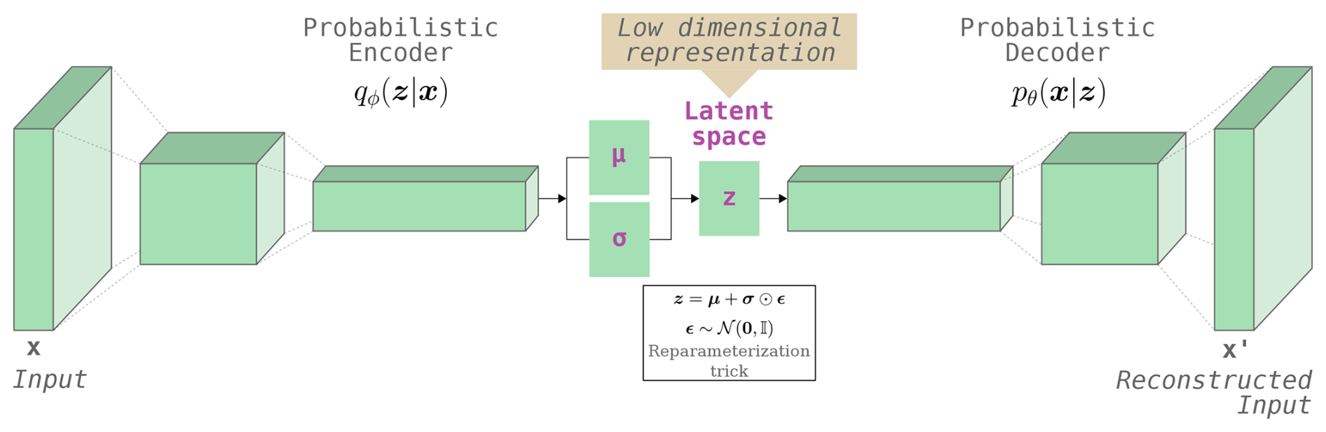
Figure 1 The basic scheme of a VAE composed of two-dimensional convolutional layers (Conv2D). The encoder compresses an input vector x into the low-dimensional latent space. The decoder attempts to reconstruct the original data from a lower-dimensional vector z sampled from the latent space. For illustrative purposes, the encoder and decoder are shown with two hidden layers, representing the progressive dimensionality reduction and expansion. In this work, we used three (synthetic experiment) and four (Etna experiment) hidden layers for the encoder and decoder.

The training of the VAE is guided by a loss function (ℒ_VAE) that balances the fidelity of the data reconstruction against a term that regularizes the probability distributions in the latent space towards a simple prior distribution p(z):

$$\begin{array}{}\text{(1)}& \begin{array}{rl}{\mathcal{L}}_{\mathrm{VAE}}& ={\mathcal{L}}_{\mathrm{R}}+{\mathcal{L}}_{\mathrm{KL}}=-{\mathbb{E}}_{q_{\mathit{\varphi }}\left(\mathit{z}\mathrm{|}\mathit{x}\right)}\left[\log p_{\mathit{\theta }}\left(\mathit{x}\mathrm{|}\mathit{z}\right)\right]\\ & +D_{\mathrm{KL}}\left(q_{\mathit{\varphi }}\left(\mathit{z}\mathrm{|}\mathit{x}\right)\parallel p\left(\mathit{z}\right)\right)\end{array}\end{array}$$

where q_ϕ(z|x) is the encoder approximate posterior and p_θ(x|z) the decoder likelihood. The first term (ℒ_R, reconstruction loss) encourages reconstructions to be accurate and, in this work, the loss function is assumed to be the Mean Squared Error (MSE) between the input (x) and its reconstructed output (x^′):

$$\begin{array}{}\text{(2)}& {\mathcal{L}}_{\mathrm{R}}={\displaystyle \frac{\mathrm{1}}{N}}\sum _{i=\mathrm{1}}^N(x_i-x_i^{\prime }{)}^{\mathrm{2}}\end{array}$$

being N the dimension of the original space. The second term (ℒ_KL) defines the loss function in terms of the Kullback-Leibler divergence (D_KL), which measures the distance between the approximate posterior q_ϕ(z|x) and the prior distribution p(z). In practice, the D_KL term forces q_ϕ to be close to the prior distribution p(z). Traditionally, the standard VAE assumes a diagonal multivariate normal distribution for the approximate posterior, $q_{\mathit{\varphi }}\left(\mathit{z}\mathrm{|}\mathit{x}\right)=\mathcal{N}(\mathit{\mu },{\mathit{\sigma }}^{\mathbf{2}}\mathbb{I})$, and a standard normal distribution for the prior, $p\left(\mathit{z}\right)=\mathcal{N}(\mathbf{0},\mathbb{I})$, leading to:

$$\begin{array}{}\text{(3)}& {\mathcal{L}}_{\mathrm{KL}}=-{\displaystyle \frac{\mathrm{1}}{\mathrm{2}}}\sum _{i=\mathrm{1}}^K\left[\mathrm{1}+\log {\mathit{\sigma }}_i^{\mathrm{2}}-{\mathit{\mu }}_i^{\mathrm{2}}-{\mathit{\sigma }}_i^{\mathrm{2}}\right]\end{array}$$

where $\mathit{\mu }=({\mathit{\mu }}_{\mathrm{1}},\mathrm{\dots },{\mathit{\mu }}_K{)}^{⊺}$ is the vector of means, ${\mathit{\sigma }}^{\mathbf{2}}=({\mathit{\sigma }}_{\mathrm{1}}^{\mathrm{2}},\mathrm{\dots },{\mathit{\sigma }}_K^{\mathrm{2}})$ is the vector of variances, and K the dimension of the latent space where vectors z live. In addition, this work uses the so-called β-VAE, a modification of the standard VAE that introduces a hyper-parameter β to weight the ℒ_KL term in the global VAE loss function:

$$\begin{array}{}\text{(4)}& {\mathcal{L}}_{\mathrm{VAE}}={\mathcal{L}}_{\mathrm{R}}+\mathit{\beta }{\mathcal{L}}_{\mathrm{KL}}\end{array}$$

Larger values of β increasingly regularize the latent space towards the standard Gaussian prior 𝒩(0,𝕀), potentially reducing the amount of information encoded in the latent representation. In summary, the VAE training step optimises the encoder and the decoder by minimising the VAE loss function Eq. (4) on a training set of input vectors {x_i}, so that inputs are accurately reconstructed from latent samples, while the latent distribution remains close to the prior. Details on VAE network architecture and hyper-parameter values are given in Sect. 4.4.

3 Latent-space data assimilation

Data Assimilation (DA) techniques aim to obtain an optimal state of a dynamical system by combining model forecasts with observations, and are widely used by operational centres to forecast geophysical systems (Carrassi et al., 2018). However, the application of DA to geophysical systems is challenging because their system states are typically represented by very high-dimensional vectors. As the dimensionality of a system increases, DA methods become increasingly difficult to apply due to the complexity of representing the system state and its associated uncertainties. Ensemble-based DA methods partially address the issue of high-dimensionality by representing the uncertainty of the system state through a finite ensemble of model realizations. The key underpinning concept is that the ensemble can approximate the relevant error statistics, making ensemble-based methods practical for high-dimensional and non-linear geophysical systems. Still, in many geoscientific applications, the computational cost of the physical models constrains the ensemble sizes, increasing sampling errors in the estimation of ensemble statistics and potentially leading to suboptimal analyses.

These limitations are particularly relevant for atmospheric applications, where the system state may comprise millions of degrees of freedom, while non-linear dynamics and non-Gaussian error distributions can limit the applicability of traditional DA approaches. For example, many variational and Kalman filter methods rely on assumptions of approximately Gaussian error statistics, leading to inaccurate state estimates when the underlying distributions are strongly non-Gaussian. Particularly challenging for DA are variables that are lower-bounded (e.g. cannot take negative values) and poorly described by Gaussian distributions, such as water-vapour mixing ratios (Kliewer et al., 2016), rainfall (Husak et al., 2007), aerosol concentrations (O'Neill et al., 2000), and volcanic ash concentrations (Mingari et al., 2023), often exhibiting strongly skewed and near-zero distributions. Particle filters circumvent the Gaussian assumption by representing the state distribution with a set of weighted samples (particles) and updating their weights according to the observation likelihood. However, as the number of state variables grows, particle weights can collapse onto one or a few particles, leading to severe particle degeneracy.

The low-dimensional manifold learned by the VAE can be exploited to perform DA in a compressed representation of the model state, expressed in terms of a relatively small number of latent variables while retaining the main spatial structures and variability of the original fields. Thus, rather than applying DA directly to the high-dimensional ash concentration fields, the analysis is performed in the latent space, reducing the dimensionality of the problem and then using the VAE decoder to map the resulting states back to the physical space. The application of ensemble-based DA methods in the VAE latent space offers several advantages. First of all, the low dimensionality of the latent representation substantially reduces the computational cost of the DA analysis, making it possible to use larger ensembles than in the original physical space. In turn, larger ensembles can potentially reduce sampling errors in the estimation of ensemble statistics. On the other hand, the compact latent representation facilitates the estimation of these statistics, while the approximately Gaussian distribution of the latent variables makes the latent space particularly suitable for ensemble-based DA methods based on Gaussian assumptions. In this work, we investigate two ensemble-based DA approaches operating in the VAE latent space: the Ensemble Transform Kalman Filter (ETKF) and the regularized bootstrap Particle Filter (PF), briefly described below.

3.1 Ensemble formulation

Let {z_i} denote a prior ensemble of N_E latent-space vectors, with z_i∈ℝ^K, and let y_obs∈ℝ^M denote the vector of M observations. The latent-space ensemble is mapped to the physical space through the VAE decoder D,

$$\begin{array}{}\text{(5)}& {\mathit{x}}_i=D\left({\mathit{z}}_i\right)\end{array}$$

with x_i∈ℝ^N. The corresponding observation-space ensemble is then obtained by applying the observation operator,

$$\begin{array}{}\text{(6)}& {\mathit{y}}_i=H\left({\mathit{x}}_i\right)=H\left(D\right({\mathit{z}}_i\left)\right),\end{array}$$

where H is the operator mapping the physical state to the observation space. Thus, although the analysis is performed in the K-dimensional latent space, the observations are related to the latent variables through the composition of the VAE decoder and the observation operator.

The prior ensemble mean in latent space is defined as

$$\begin{array}{}\text{(7)}& \overline{\mathit{z}}={\displaystyle \frac{\mathrm{1}}{N_{\mathrm{E}}}}\sum _{i=\mathrm{1}}^{N_{\mathrm{E}}}{\mathit{z}}_i\end{array}$$

We define the background anomaly matrix ${\mathbf{Z}}^{\prime }\in {\mathbb{R}}^{K\times N_{\mathrm{E}}}$, whose ith column represents the deviation of the corresponding ensemble member from the ensemble mean, ${\mathit{z}}_i-\overline{\mathit{z}}$. Similarly, we define the observation-space anomaly matrix ${\mathbf{Y}}^{\prime }\in {\mathbb{R}}^{M\times N_E}$, whose columns represent the deviations of the observation-space ensemble members from the corresponding ensemble mean, ${\mathit{y}}_i-\overline{\mathit{y}}$.

3.2 Ensemble transform Kalman filter

The Ensemble transform Kalman filter (ETKF), introduced by Bishop et al. (2001), is employed in this work following the formulation adopted by Hunt et al. (2007). The analysis ensemble is obtained by updating both the prior ensemble mean ($\overline{\mathit{z}}\to {\overline{\mathit{z}}}_a$) and the prior ensemble anomalies (${\mathbf{Z}}^{\prime }\to {{\mathbf{Z}}^{\prime }}_a$). The analysis ensemble mean ${\overline{\mathit{z}}}_{\mathrm{a}}$ is expressed as a linear combination of the background ensemble anomalies,

$$\begin{array}{}\text{(8)}& {\overline{\mathit{z}}}_{\mathrm{a}}=\overline{\mathit{z}}+{\mathbf{Z}}^{\prime }\mathit{w},\end{array}$$

where $\mathit{w}\in {\mathbb{R}}^{N_{\mathrm{E}}}$ is a vector of weights to be determined. In turn, the analysis anomalies ${{\mathbf{Z}}^{\prime }}_{\mathrm{a}}$ are obtained by applying a transformation matrix W to the background anomalies,

$$\begin{array}{}\text{(9)}& {{\mathbf{Z}}^{\prime }}_{\mathrm{a}}={\mathbf{Z}}^{\prime }\mathbf{W}.\end{array}$$

The weight vector w in Eq. (8) is obtained by solving the linear system

$$\begin{array}{}\text{(10)}& \mathbf{A}\mathit{w}={{\mathbf{Y}}^{\prime }}^{⊺}{\mathbf{R}}^{-\mathrm{1}}\mathit{d},\end{array}$$

where R is the observation-error covariance matrix, $\mathit{d}={\mathit{y}}_{\mathrm{obs}}-\overline{\mathit{y}}$ is the innovation vector, and the matrix A is defined as

$$\begin{array}{}\text{(11)}& \mathbf{A}=(k-\mathrm{1})\mathbf{I}+{{\mathbf{Y}}^{\prime }}^{⊺}{\mathbf{R}}^{-\mathrm{1}}{\mathbf{Y}}^{\prime }.\end{array}$$

The analysis covariance in the latent space is given by

$$\begin{array}{}\text{(12)}& {\mathbf{P}}^{\mathrm{a}}={\mathbf{Z}}^{\prime }{\mathbf{A}}^{-\mathrm{1}}{{\mathbf{Z}}^{\prime }}^{⊺}\end{array}$$

In order to obtain an ensemble with this covariance, the transformation matrix W in Eq. (9) is constructed as a symmetric square root of $(N_{\mathrm{E}}-\mathrm{1}){\mathbf{A}}^{-\mathrm{1}}$. Specifically, using the eigendecomposition $\mathbf{A}=\mathbf{V}\mathbf{\Lambda }{\mathbf{V}}^{⊺}$ the transformation matrix W is given by

$$\begin{array}{}\text{(13)}& \mathbf{W}=\sqrt{N_{\mathrm{E}}-\mathrm{1}}\mathbf{V}{\mathbf{\Lambda }}^{-\mathrm{1}/\mathrm{2}}{\mathbf{V}}^{⊺}\end{array}$$

This transformation ensures that the sample covariance of the analysis ensemble is consistent with P^a. The posterior latent ensemble members are obtained from Eqs. (8) and (9) by adding the transformed anomalies to the analysis mean. Finally, the resulting set of vectors z_a are then be passed through the VAE decoder to obtain the corresponding physical-space ensemble resulting from the analysis step.

3.3 Regularized bootstrap particle filter

Particle filtering (Doucet et al., 2001) has been successfully applied to low-dimensional models, e.g. in non-linear tracking problems (Arulampalam et al., 2002), but direct application of the basic PF to high-dimensional systems is prone to weight collapse, as discussed previously. As a result, several variants have been proposed to enable the application of particle filters in geophysical systems (van Leeuwen, 2009). Since the dimensionality of the latent space is substantially lower than that of the original physical space, we explore whether particle filtering becomes a viable option for data assimilation in this reduced representation. In this work, a basic bootstrap particle filter (Gordon et al., 1993) with Gaussian kernel regularization (Pham, 2001) is tested for latent-space data assimilation. The particle weights are computed from the observation likelihood,

$$\begin{array}{}\text{(14)}& w_i\propto p\left({\mathit{y}}_{\mathrm{obs}}\mid {\mathit{y}}_i\right),\end{array}$$

and normalized to sum to one. The particles are then resampled according to their weights using systematic resampling (Kitagawa, 1996), producing an equally weighted ensemble of size N_E. When the particle weights are highly concentrated on a small number of particles, resampling can substantially reduce the diversity of the ensemble. To restore particle diversity, the resampled particles, ${\mathit{z}}_i^{\mathrm{r}}$, are subsequently perturbed using a Gaussian kernel,

$$\begin{array}{}\text{(15)}& {\mathit{z}}_i^{\mathrm{a}}={\mathit{z}}_i^{\mathrm{r}}+{\mathit{ϵ}}_i,{\mathit{ϵ}}_i\sim \mathcal{N}(\mathbf{0},{\mathbf{\Sigma }}_{\mathrm{reg}}),\end{array}$$

where Σ_reg=h²P, with P the sample covariance of the prior latent ensemble and h a prescribed regularization factor. This kernel perturbation provides a simple regularization aimed at increasing the diversity among the resampled particles.

4 Numerical experiments and evaluation

Two types of numerical experiments were performed: (i) a synthetic experiment (Mingari, 2026b) to characterize the VAE-generated ensemble and assess its ability to reproduce the statistics of a physics-based reference ensemble; and (ii) a second experiment (Mingari, 2026a) considering a real-case application aimed at improving the modelling of volcanic clouds through data assimilation in the latent space. The code and the material required to reproduce both experiments are available in the Supplement.

4.1 Physics-based atmospheric dispersal model

The latest release (version 9.1) of the open-source code FALL3D (Folch et al., 2025) was used to produce an ensemble of numerical simulations for the two experiments. The resulting datasets were then used for VAE training, testing and evaluation. FALL3D is an Eulerian model for atmospheric passive transport and deposition of different atmospheric species (e.g., volcanic ash and gases, mineral dust and radionuclides) based on the so-called Advection-Diffusion-Sedimentation (ADS) equation (Folch et al., 2020; Prata et al., 2021). The numerical model is GPU-accelerated using the OpenACC parallel programming model and has been designed to support increasingly larger scientific workloads in preparation for the transition to extreme-scale computing systems (Folch et al., 2023). The FALL3D model has been deployed and optimised on several EuroHPC supercomputing systems: LUMI (Finland), Leonardo (Italy), and MareNostrum-5 (Spain), covering both NVIDIA and AMD GPU architectures. FALL3D is designed to run ensemble simulations as a single, massively parallel job, allowing to maximize computational efficiency and scalability (Folch et al., 2022). Broadly speaking, ensemble modelling allows to characterise and quantify model uncertainties due to poorly constrained input parameters and errors in the numerical model, physical parameterisations or underlying model-driving meteorological data. In addition, the ability to generate ensemble runs makes it possible to improve forecasts by incorporating observations using different ensemble-based data assimilation techniques. The configuration of the FALL3D model for the two experiments is summarised in Table 1.

4.2 Synthetic experiment

To define the first experiment, we used model data from the recent EU-MODEX Tenerife 2025 exercise (European Commission, 2025), organised under the European Civil Protection Mechanism. This exercise represented the first large-scale volcanic eruption drill in Spain to practice the response to a potential volcanic eruption from Garachico volcano (Tenerife, Canary Islands) and test the evacuation, the social assistance and communication protocols during a volcanic crisis. On 26 September 2025, we provided real-time ash-dispersion forecasts for a hypothetical eruption scenario to support emergency decision-making. Here we use the resulting simulations to characterize the statistical properties of an augmented ensemble generated by the VAE in a controlled experiment. In this context, the drill scenario refers to a fictitious eruption defined by given emission source parameters (eruption column height, mass eruption rate, and timing), rather than being constrained by real-time observations as would happen during a real event. Since our study focuses on generating ensembles from numerical simulations and approximating their statistical distribution, the distinction between real and hypothetical eruption scenarios does not affect the methodology or conclusions. This case was deliberately selected because the ensemble simulations produce qualitatively different plume transport patterns, providing a suitable test bed to inspect the ability of the VAE to reproduce the variability and statistical characteristics of the simulated ensemble.

Three ensembles were simulated with FALL3D to produce the training, validation, and test datasets. The training ensemble, consisting of 256 members, was used to train the VAE and the validation ensemble, consisting of 64 members, was used during the training step to monitor the performance and tuning of the neural network hyper-parameters. Finally, the larger test ensemble, consisting of 2048 members, was used only at the end as a purely physics-based reference to evaluate the VAE model, providing a fair (unbiased) report of model accuracy. All numerical simulations were performed on the LUMI supercomputing system, hosted at the Finish CSC. In particular, the execution of the test ensemble required substantial HPC resources and was executed on the LUMI-G partition allocating 256 computing nodes and a total of 2048 GPUs (one per ensemble member). In all cases, a 24 h time window forecast was performed assuming a continuous ash emission starting at 09:00 UTC (see Table 1), a local-scale computational domain with a horizontal resolution of 0.1° and 120 × 100 × 25 grid cells, and the FALL3D dispersal model was driven by the Global Forecast System (GFS) weather forecast from the National Centers for Environmental Prediction (NCEP). Each ensemble was simulated by perturbing Eruption Source Parameters (ESPs) and wind components, which are widely recognized as among the most sensitive parameters/inputs for volcanic ash transport models (Devenish et al., 2012; Poulidis et al., 2018). The column height was sampled around a central value of 9 km above the vent level. Further details on the perturbed parameters and sampling ranges are provided in the Supplement.

Table 1 FALL3D model configurations used in the numerical experiments.

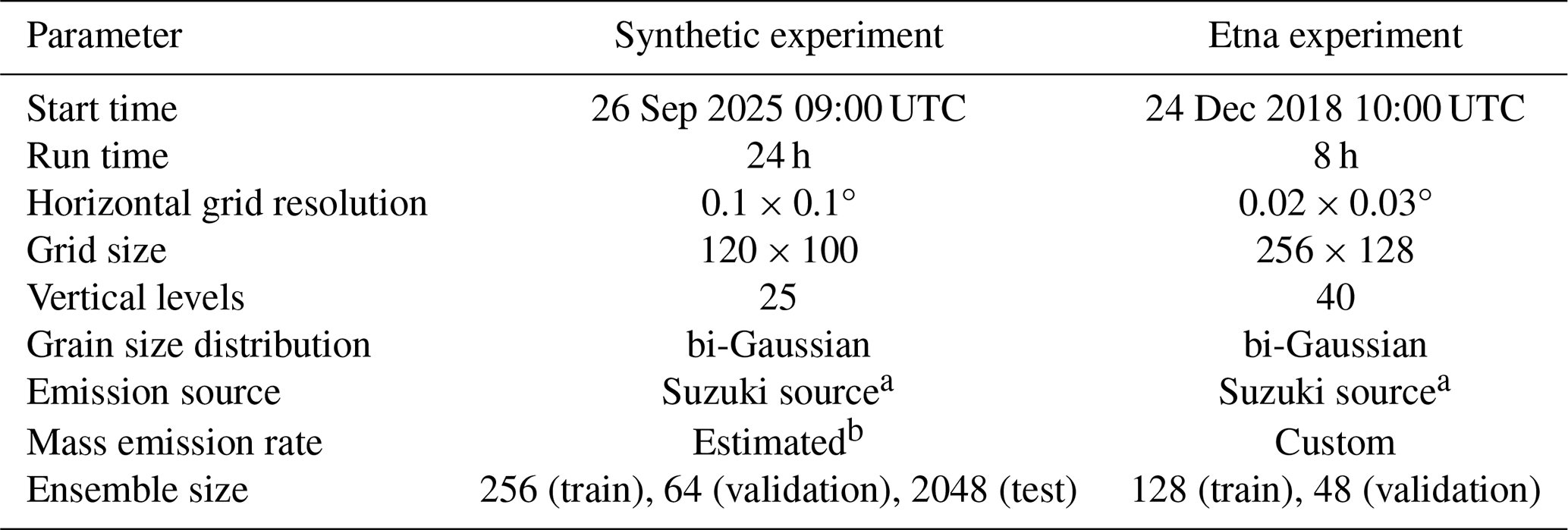
^a Suzuki source formulation following Pfeiffer et al. (2005); ^b Mass emission rate computed following Woodhouse et al. (2016).

4.3 Etna experiment

The second experiment explores the feasibility of the latent-space DA using a VAE-generated prior ensemble for the 24 December 2018 Etna eruption (Corradini et al., 2020; Pardini et al., 2020). In this case, the FALL3D model was driven by the Copernicus regional reanalysis for Europe (CERRA; Schimanke et al., 2021; Ridal et al., 2024), with 106 vertical model levels, and initialized at 10:00 UTC. An 8 h time window forecast was performed using a 128-member ensemble (model prior). An additional 48-member ensemble was simulated to be used as a validation dataset during the training process (see Table 1). Each ensemble was simulated by perturbing the eruptive column-top height and wind components by 20 % (see Supplement for further details).

The 128-member model prior was used to train a new VAE, which was subsequently used to sample a 4096-members ensemble (VAE prior) for the analysis step. As a proof-of-concept, we used two-dimensional ash column-mass fields rather than the full three-dimensional concentration field, both to reduce the dimensionality of the problem and to maintain a consistent neural-network architecture throughout the study. The input training data, defined on a 256 × 128 grid (N= 131 072), was encoded into 32-dimensional latent space vectors. Before normalization, a log (1+x) transformation was applied to the ash column mass (x) to reduce the strong positive skewness of its distribution, with x expressed in mg m⁻².

A single analysis step at 18:00 UTC was performed by assimilating Spinning Enhanced Visible and Infra-Red Imager (SEVIRI) volcanic ash retrievals (Corradini et al., 2020, 2021) considering two ensemble-based approaches, i.e., the ETKF (Sect. 3.2) and the PF (Sect. 3.3). Only positive retrievals were considered, resulting in 2678 valid observations of ash column mass. A diagonal observation-error covariance matrix was assumed, with the observation-error standard deviation set to 50 % of the retrieved ash column mass, subject to a minimum value of 100 mg m⁻², representative of a typical instrument detection limit.

4.4 VAE configuration

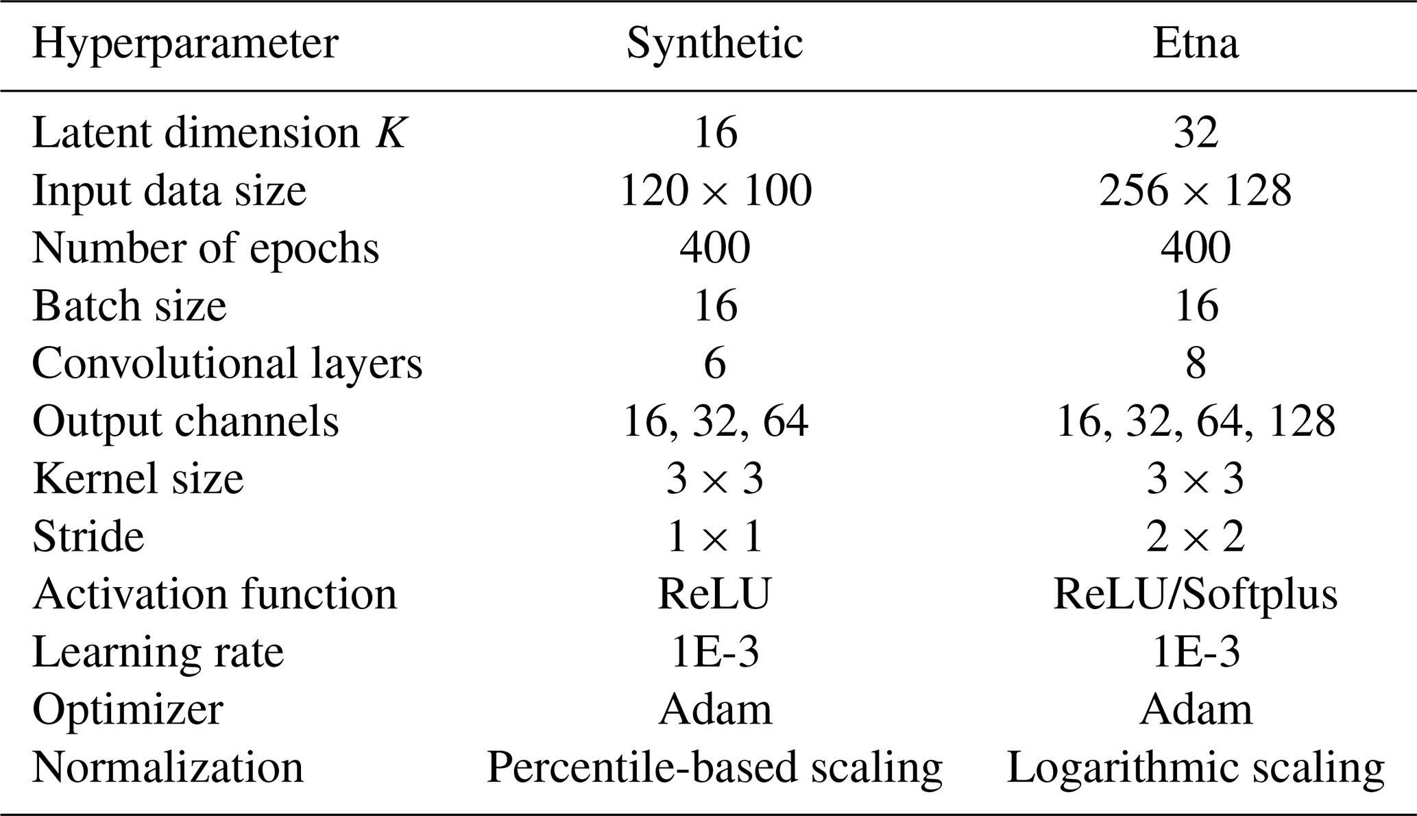
A VAE was implemented in the PyTorch framework (Paszke et al., 2019) using an architecture based on two-dimensional convolutional layers with kernel size of 3 × 3. The VAE configuration is defined by the hyperparameters reported in Table 2. The resulting number of trainable parameters was 698 849 and 1 783 489 for the synthetic and the Etna experiments respectively. The neural network was trained using the Adam optimizer during 400 epochs using mini-batches of 16 samples. The reconstruction loss and KL divergence (averaged over batches) were monitored at each epoch for both the training and validation datasets to prevent overfitting. Training was performed using the simulated ensembles of two-dimensional volcanic ash column-mass fields at a single forecast time. As outlined in Fig. 1, the encoder network maps the input data x through successive convolutional layers, followed by a flattening operation to two distinct latent space parameter vectors μ (mean) and log σ² (log-variance), with dimensions K=16 and K=32 for the synthetic and Etna experiments, respectively. The decoder then reconstructs the input from the sampled latent vector z using a fully connected layer followed by successive upsampling and convolutional operations, restoring the original spatial dimensions. For the synthetic experiment, transposed convolutional layers are used for upsampling, whereas bilinear interpolation followed by convolutional layers is used in the Etna experiment to reduce checkerboard artifacts.

Table 2 Hyper-parameters used for the VAE training in the synthetic and Etna experiments.

4.5 Evaluation metrics

4.5.1 Standard performance metrics

The performance of the generated ensembles is evaluated in terms of a set of statistical metrics. Let x and $\widehat{\mathit{x}}$ denote the reference and estimated quantities, respectively, with N denoting the total number of values being compared. The root mean square error (RMSE) is defined as

$$\begin{array}{}\text{(16)}& \text{RMSE}=\sqrt{{\displaystyle \frac{\mathrm{1}}{N}}\sum _{j=\mathrm{1}}^N(x_j-{\widehat{x}}_j{)}^{\mathrm{2}}}.\end{array}$$

The root mean square logarithmic error (RMSLE) is computed analogously after applying the logarithmic transformation log (1+x), providing a metric more sensitive to errors across multiple orders of magnitude. Similarly, the Mean Bias Error (MBE) is computed as

$$\begin{array}{}\text{(17)}& \text{MBE}={\displaystyle \frac{\mathrm{1}}{N}}\sum _{j=\mathrm{1}}^N{x}_j-{\widehat{x}}_j\end{array}$$

The Mean Absolute Percentage Error (MAPE) provides another relative measure of accuracy:

$$\begin{array}{}\text{(18)}& \text{MAPE}=\mathrm{100}\times \sum _{j=\mathrm{1}}^N\left|{\displaystyle \frac{x_j-{\widehat{x}}_j}{{\widehat{x}}_j}}\right|\end{array}$$

Finally, the Pearson correlation coefficient measures the linear correlation between the estimated and reference fields.

4.5.2 Distributional assessment

In addition to the standard performance metrics introduced above, the ability of the VAE to reproduce the statistical properties of the target distribution is further assessed using distributional and spectral metrics. The Jensen-Shannon (JS) divergence is a measure of the similarity between two probability distributions. Specifically, for two distributions P={p_i} and Q={q_i}, the JS divergence is a symmetrized version of the KL divergence:

$$\begin{array}{}\text{(19)}& \mathrm{JSD}(P\parallel Q)={\displaystyle \frac{\mathrm{1}}{\mathrm{2}}}{D}_{\mathrm{KL}}(P\parallel M)+{\displaystyle \frac{\mathrm{1}}{\mathrm{2}}}{D}_{\mathrm{KL}}(Q\parallel M)\end{array}$$

where $M=\frac{\mathrm{1}}{\mathrm{2}}(P+Q)$ is a mixture distribution of P and Q, while D_KL can be interpreted as the expected logarithmic difference between the probability distributions (Goodfellow et al., 2016):

$$\begin{array}{}\text{(20)}& D_{\mathrm{KL}}(P\parallel Q)=\sum p_i\log {\displaystyle \frac{p_i}{q_i}}\end{array}$$

The discrete distributions in Eq. (20) are estimated from histograms in this work.

The two-dimensional isotropic power spectrum, P(k), was also computed to assess the ability of the VAE to generate realistic samples over different spatial scales, in consistency with physically-based models. This power spectrum is defined as the radially-averaged 2D Power Spectrum Density (PSD) and is a function of the wavenumber magnitude, k:

$$\begin{array}{}\text{(21)}& P\left(k\right)={\displaystyle \frac{\mathrm{1}}{N_k}}\sum \mathrm{PSD}(k_x,k_y)\end{array}$$

where $k=\sqrt{k_x^{\mathrm{2}}+k_y^{\mathrm{2}}}$ is the magnitude of the wavevector, PSD(k_x,k_y) is the two-dimensional Power Spectral Density obtained from a Fast Fourier Transform (FFT), and N_k is the number of data points within an annular ring around k in the Fourier space.

4.5.3 Categorical metrics

Categorical metrics were also used to assess binary plume detection. A positive detection is defined when the ash column mass exceeds a given threshold, set to 100 mg m⁻² in this work for demonstration purposes, which is a typical value corresponding to the satellite detection limit for ash clouds. The probability of detection (POD) measures the fraction of observed plume grid points that are correctly identified,

$$\begin{array}{}\text{(22)}& \mathrm{POD}={\displaystyle \frac{\mathrm{TP}}{\mathrm{TP}+\mathrm{FN}}},\end{array}$$

where TP and FN denote true positives and false negatives, respectively. The Jaccard index measures the spatial overlap between the plume masks,

$$\begin{array}{}\text{(23)}& J={\displaystyle \frac{\mathrm{TP}}{\mathrm{TP}+\mathrm{FP}+\mathrm{FN}}},\end{array}$$

where FP denotes false positives. In summary, the probability of detection (POD) and Jaccard index were used to quantify the detection skill and spatial overlap, respectively.

5 Results and discussion

This section presents the results organized as follows. First, in Sect. 5.1, the synthetic experiment is used to assess the consistency of the VAE training, as well as to perform a sensitivity study to determine the most appropriate configuration. Second, Sect. 5.2 evaluates the capability of the VAE-generated ensemble to reproduce the statistical properties of a larger physics-based ensemble. To this end, a test dataset comprising 2048 FALL3D simulations was generated for the synthetic experiment, serving as a reference for comparison. Third, Sect. 5.3 illustrates a real-case application of this methodology using the Etna experiment: the latent-space assimilation of satellite observations. Finally, the implications of these results and the main limitations of the proposed approach are discussed in Sect. 5.4.

5.1 Training sensitivity analysis

A sensitivity analysis was conducted to evaluate the performance of different neural network configurations trained with the synthetic experiment datasets. Multiple VAE configurations were trained by exploring a range of values for two key hyper-parameters: the latent space dimension K and the factor β in Eq. (4), while fixing the remaining hyper-parameters with the values specified in Table 2. For each trained VAE, an ensemble was generated by independently sampling latent vectors from the standard normal distribution and decoding them to recover the corresponding physical-space variables. In this section, each generated ensemble consisted of 2048 members.

The performance was evaluated in terms of the RMSE using Eq. (16), computed between the ensemble mean of the test dataset (taken as the reference) and the means of the VAE-generated ensembles. To account for the stochastic variability of the VAE generation, 20 ensembles were generated for each set of hyper-parameters tested. The resulting RMSE values are shown as box plots in Fig. 2. In all cases, the network was trained for 400 epochs, except for configurations with latent dimensions of K=4 and K=2, where early stopping was required to avoid overfitting. According to the trend suggested by Fig. 2, the best performance is achieved for latent dimensions K≳6 and β≳6. Remarkably, performance degrades slightly for large latent space dimensions (Fig. 2a). There are two possible explanations for this anomaly. First, large latent spaces often produce less stable training dynamics and worse generalization: enlarging latent spaces introduces more degrees of freedom than the data can realistically support. When the dimensionality grows beyond what is needed to represent the underlying factors, the model may spread information across latent variables in an inefficient way. This leads to poor compression, weaker regularization and a latent representation that becomes harder to structure during training, limiting the extraction of compact and meaningful representations. As a result, the decoder receives a less informative latent code, reducing the reconstruction quality. On the other hand, increasing the latent dimensionality can slow convergence: since the model must explore a much larger parameter space before reaching a stable configuration, it requires more training iterations and makes optimisation more difficult.

In addition, Fig. 2 shows also the impact of the β parameter, which controls the strength of the KL regularization in the loss function and, therefore, the balance between reconstruction fidelity and latent-space structure. Higher values force the model to impose a tighter, more organised latent space, at the expense of losing some fine-scale details in the reconstructions. In our case, β≈6 suggests that a strongly regularised latent representation is more beneficial for the task than capturing every small feature in the input data. This indicates that the model gains more from enforcing a well-structured latent space than from preserving high-resolution details during reconstruction.

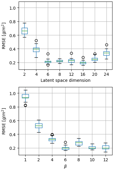
Figure 2 VAE sensitivity analysis for different combinations of two hyper-parameters: the latent space dimension K (top) and the β parameter (bottom), defined in Eq. (4). The performance is measured in terms of the Root-Mean-Square Error (RMSE), computed from the ensemble means. The boxes show the interquartile range, the horizontal lines indicate the median, and the circles represent outliers.

This is further supported by the structure of the latent space shown in Fig. 3. The nearly diagonal covariance matrix (Fig. 3a) indicates weak correlation between the latent components, consistent with a well-regularized latent representation. Figure 3b shows a two-dimensional visualization of the latent space based on the Uniform Manifold Approximation and Projection (UMAP) algorithm (McInnes et al., 2020), a technique for non-linear dimensionality reduction specifically designed to preserve the local structure of the data. The UMAP projection shows that the test dataset (circular markers) occupies the same region of latent space than the training data (plus-shaped markers), indicating that the learned representation generalizes to unseen data, rather than only organizing the training samples. In addition, it is also worth showing how the encoding can discriminate between qualitatively different model solutions (ensemble members) by grouping them in different regions of the latent space. This is illustrated in Fig. 3b by means of coloured-scale dots, where members with eruption column heights higher and lower than the reference (ensemble central member) are clearly concentrated in disjoint (i.e. non-overlapping) regions of latent space. In other words, the VAE encoding implicitly produces a latent space with a clustering-like structure. These results indicate that the network was trained correctly and behaves as expected. Based on this sensitivity analysis, a latent dimension of K=16 and β=6 were adopted for the VAE configuration used in the next section.

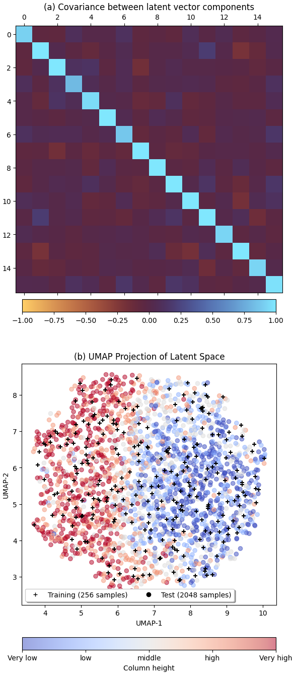
Figure 3 Structure of the latent space for K=16 and β=6. The independence between the distributions of the latent vector components can be confirmed from the covariance matrix (a). The test dataset is encoded in the same region of the latent space covered by the training dataset, as shown in the UMAP two-dimensional visualization of the latent space (b), confirming that the learned representation generalizes well to unseen data. See text for details.

5.2 Evaluation of the VAE-generated ensemble

Once the VAE neural network is properly trained, new samples (ensemble members) can be generated at negligible computational cost. This section explores whether these VAE-generated samples can reproduce the statistical characteristics of an independent and larger ensemble of numerical simulations (test dataset from the synthetic experiment), even when the new samples have not been obtained by explicitly solving the underlying physical equations. For illustrative purposes, Fig. 4 shows a few VAE-generated samples of two-dimensional ash column mass. The variability in the ensemble is a consequence of the different eruptive source parameters (e.g., eruptive column height) and meteorological conditions used to simulate the training dataset. For example, samples in Fig. 4c,d correspond to cases with high eruptive column heights and strong emission, whereas other samples are associated with low column heights and weak emission (e.g. Fig. 4h). In most cases, the volcanic plume is advected eastwards from the vent (16.76° W, 28.27° N). Additionally, some cases are characterised by a secondary plume with a SE- or even W-component in the transport pattern, suggesting the presence of strong wind shear that introduces variability into the ensemble and leads to qualitatively different solutions.

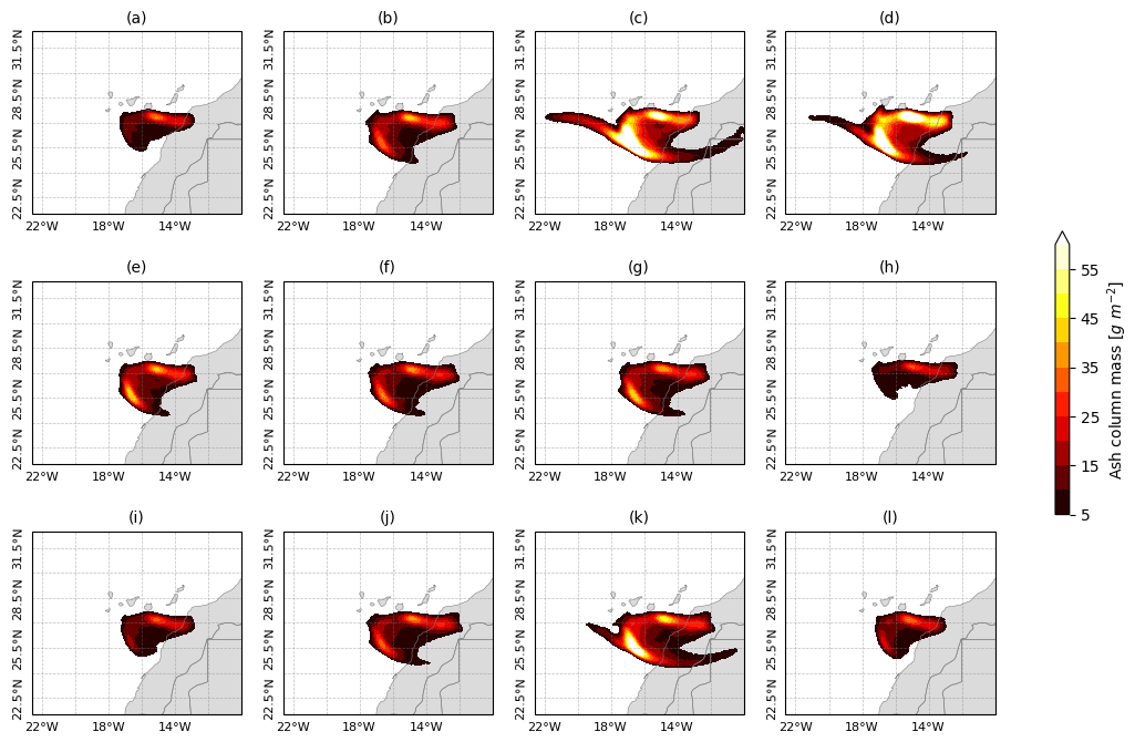
Figure 4 The neural network was trained to generate samples of two-dimensional ash column mass, i.e. the total mass of volcanic ash in a vertical column. In this example, a VAE-generated ensemble composed of 12 samples is shown.

5.2.1 Ensemble mean and spread

The VAE ability to reproduce sample statistics, such as the ensemble mean and spread (standard deviation), is examined in this section and a few metrics are reported. Figure 5 compares the ensemble means of the training ensemble (Fig. 5a) and VAE-generated ensemble comprising 5000 members (Fig. 5b). Ideally, VAE should be able to closely approximate the test dataset (reference) to achieve good performances. Deviations from the reference test dataset are quantified by bias maps. In relative terms, the bias is small for both the training dataset (Fig. 5c) and VAE (Fig. 5d), although the training dataset provides a slightly better estimate of the ensemble mean in general.

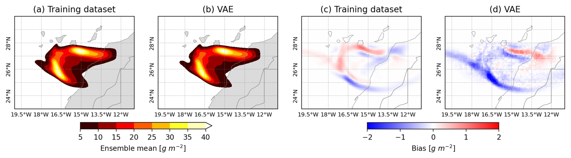
Figure 5 Ensemble mean maps obtained from the training dataset (a) and a VAE-generated ensemble with 5000 samples (b). The bias maps for the training (c) and VAE (d) ensemble means are computed by subtracting the reference (test dataset) corresponding results.

A summary of the metrics for the ensemble mean and spread is shown in Table 3. Metrics are computed for multiple VAE-generated ensembles composed of 5000 samples in order to account for the variability introduced by stochastic sampling. The average over 20 ensembles is reported along with the standard deviation for the uncertainty. The test dataset (2048 members) is taken as a reference in order to evaluate each of the metrics described in Sect. 4.5. Note that the VAE errors measured in terms of the RMSE are twice as high as those from the training dataset (256 members). In relative terms, this represents an error of 1.78 % (training) and 3.4 % (VAE) according to the MAPE evaluated from the ensemble mean. In order to avoid divisions by zero and numerical instabilities, the MAPE was actually computed considering only the regions where the test dataset is above 5 g m⁻² (i.e. the range shown in Fig. 5a,b). We can conclude that the VAE-generated ensemble is properly capturing the first (mean) and second moments (variance) of the distribution, although the training estimations for the ensemble mean and spread are still slightly better. However, the next section demonstrates how, when larger ensembles are generated, the VAE tends to perform better on metrics that are more sensitive to sampling errors.

Table 3 A summary of some performance metrics evaluated using the test dataset (2048 members) as the reference. The VAE metrics were averaged over 20 ensembles generated to account for stochastic variability. The VAE uncertainty range is given by the standard deviation.

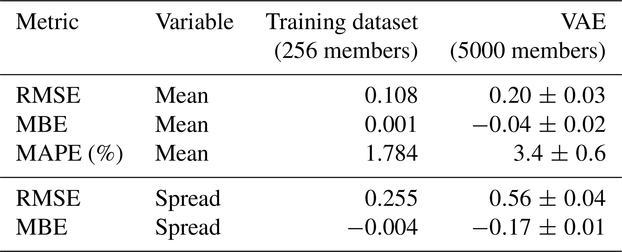
Values are reported in g m⁻², except MAPE, which is given as a percentage (%).

5.2.2 Probability distributions

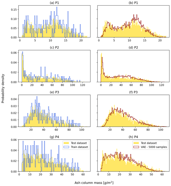
An important aspect in hazard and impact assessment is to evaluate exceedance probabilities, i.e. the probability that a specific hazardous threshold is exceeded within a given time frame. In the context of ensemble modelling, probability distribution estimations can suffer from sampling errors, particularly when small ensembles are considered. Figure 6 presents the exceedance probabilities for three different thresholds, demonstrating that a 5000-member VAE-generated ensemble can produce accurate probability distributions as well as realistic samples. In order to examine whether the sampled ensemble provides a good approximation to the reference distribution, a few histograms are shown in Fig. 7 at four selected locations, comparing results for the training dataset (left column) and a VAE ensemble with 5000 samples (right column), considering 128 bins between the minimum and maximum values for each location. As expected, the distribution estimated from the training dataset with a small ensemble size (N_E=256) results in a very noisy distribution, while the VAE distribution provides a good approximation to the test dataset distribution, even for multimodal distributions (e.g., Fig. 7a).

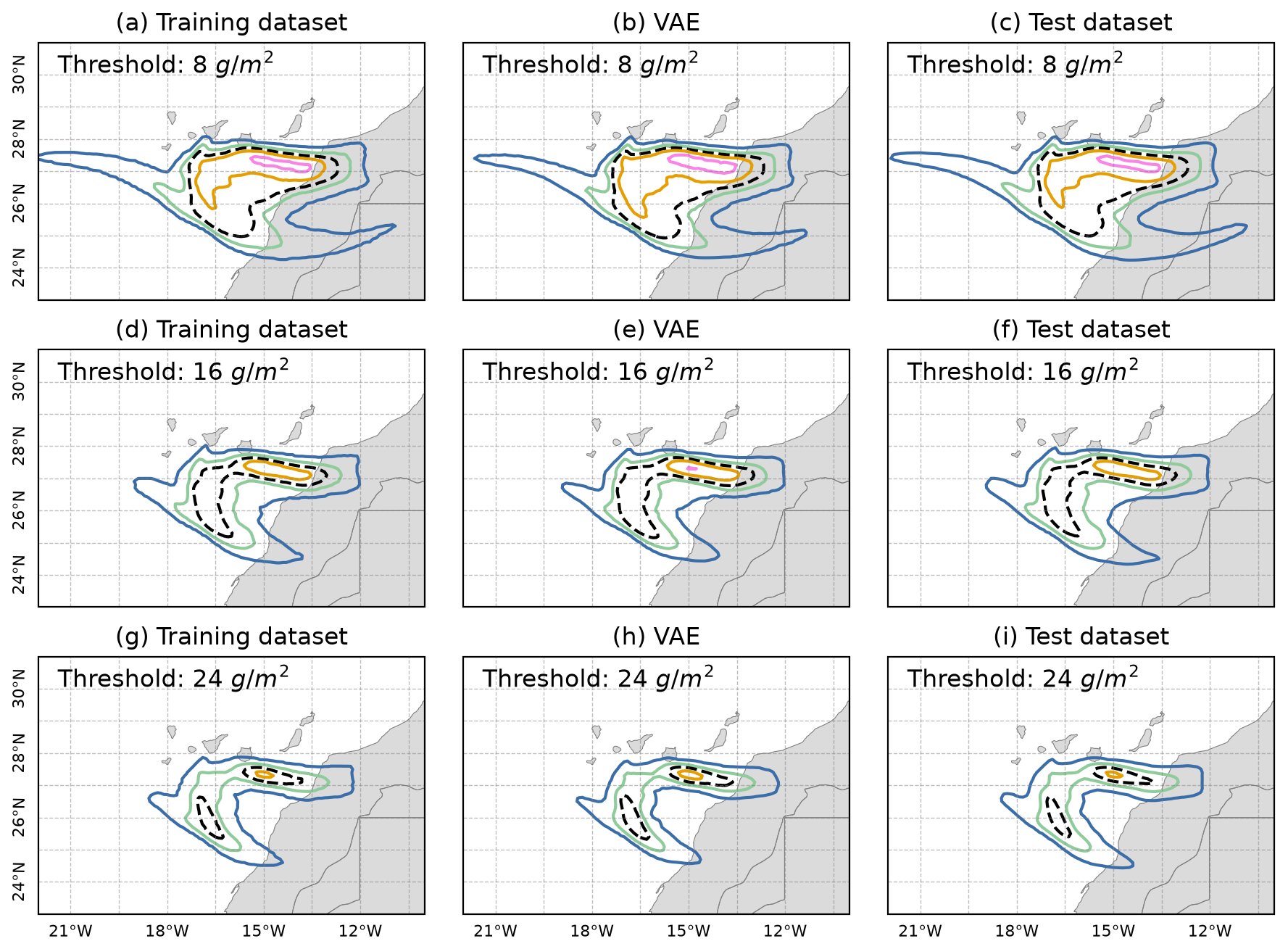
Figure 6 Exceedance probabilities for three ash column mass thresholds (8, 16 and 24 g m⁻² from top to bottom). The probability contours indicate probability levels of 2 % (blue), 25 % (green), 50 % (dashed black), 75 % (orange), and 98 % (magenta). Results for the training dataset (left column) and a VAE-generated ensemble with 5000 samples (central column) are compared with the test dataset (right column).

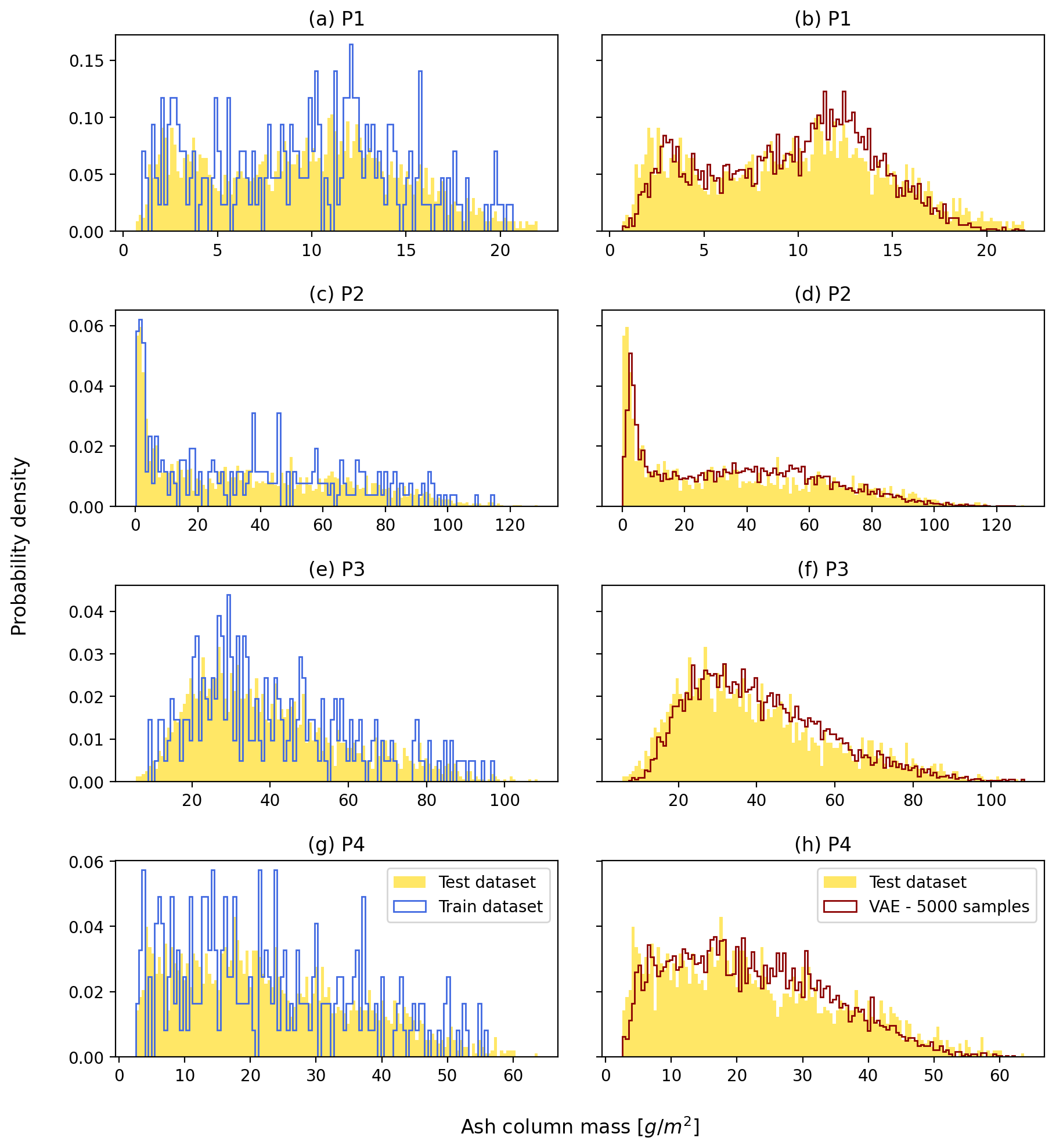
Figure 7 Histograms for the training dataset (256 samples, left column) and a VAE-generated ensemble (5000 samples, right column) at different locations. The results are compared against the test dataset (2048 samples), assumed to be the reference (yellow shaded area). For illustrative purposes, four sampling locations were selected: P1 at 15.5° W, 26.3° N (a, b); P2 at 16.8° W, 25.9° N (c, d); P3 at 15.0° W, 27.3° N (e, f); and P4 at 15.5° W, 27.4° N (g, h). See the Supplement for the point locations.

Naturally, the VAE capacity to approximate the distribution depends on the number of samples generated. In order to assess the quality of the approximation for different amounts of samples, the JS divergence was computed from discrete probability distributions using Eq. (19). Specifically, JSD was obtained from histograms with a fixed range (128 bins between 0 and 40 g m⁻²) for each grid cell. As a measure of the worst-case conditions, the 99th percentile of the grid‐cell values is reported in Fig. 8, taken as a robust estimation of the maximum JSD over the domain. The results for multiple VAE-generated ensemble sizes are compared with the training dataset. As expected, VAE improves the training distribution only for large ensemble sizes (N_E≳256), reaching an asymptotic value of approximately JSD ∼0.042, which represents a 2.6× improvement over the corresponding training metric (JSD=0.11).

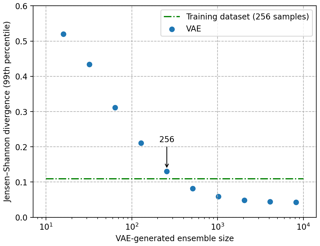
Figure 8 The Jensen-Shannon (JS) divergence was computed for each grid cell considering different sizes of the VAE-generated ensemble. The 99th percentile is reported as a worst-case measure of performance. Low values indicate a good approximation to the reference probability distribution. The result for the training dataset is also indicated for reference.

5.2.3 Isotropic power spectrum

The isotropic power spectrum, i.e. the radially averaged two-dimensional Power Spectral Density (PSD), was computed using Eq. (21). Figure 9 presents the spectra for the test dataset and VAE-generated samples, averaged over the N_E=5000 realizations of each ensemble. Unlike the classical turbulent energy-cascade spectrum, which is often characterized by a power-law dependence proportional to $k^{-\mathrm{5}/\mathrm{3}}$, the test dataset exhibits an approximately exponential decay (solid red line). This behaviour is likely related to the diffusive processes represented in the FALL3D dispersal model. The results for the transposed-convolution decoder used in the synthetic experiment are represented by green triangles in Fig. 9. The generative model reproduces the large-scale spatial structure reasonably well, but exhibits excess high-wavenumber spectral power at scales smaller than approximately 3 Δx, where Δx denotes the grid spacing, indicating the introduction of artificial small-scale noise. The flat high-wavenumber tail in the two-dimensional power spectrum may be related to the convolutional kernel size used in this work (i.e., 3 × 3) and to limitations of the decoder upsampling operation. The decoder architecture used in the synthetic experiment is based on transposed convolution layers, which are known to produce chequerboard artefacts. A similar pattern is visible in the bias map of the ensemble-mean field (Fig. 5d), where a noisy pattern with relatively low intensity and high-frequency structure can be identified. A new neural network was trained using a decoder based on bilinear interpolation for upsampling instead of transposed convolution layers, in order to investigate whether this alternative decoder architecture leads to stronger low-pass filtering (blue crosses in Fig. 9). Although deviations from the test spectrum persist for $k>\mathrm{0.33}\mathrm{\Delta }{x}^{-\mathrm{1}}$, the high-wavenumber spectral power is noticeably reduced, indicating that the bilinear-interpolation decoder provides more effective suppression of small-scale noise than the original transposed-convolution decoder. To quantify the differences at small spatial scales, we computed the fraction of total spectral power associated with wavenumbers $k>\mathrm{0.33}\mathrm{\Delta }{x}^{-\mathrm{1}}$. This fraction was 0.003 % for the test dataset, 0.020 % for the VAE with the transposed-convolution decoder, and 0.009 % for the VAE with the bilinear-interpolation decoder. In other words, the bilinear-interpolation decoder reduced the excess power by approximately 55 % relative to the transposed-convolution decoder.

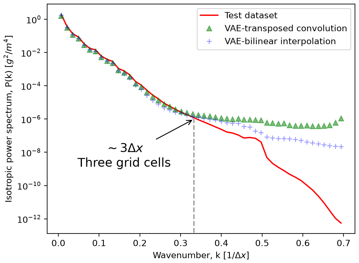
Figure 9 The isotropic power spectrum, i.e. radially averaged two-dimensional Power Spectral Density (PSD), for the test dataset and the VAE-generated samples obtained with transposed-convolution and bilinear-interpolation decoders. The generative model reproduces the large-scale spatial structure reasonably well, but exhibits excess high-wavenumber spectral power at scales smaller than approximately 3 Δx, indicating the introduction of artificial small-scale noise. This excess is more pronounced for the transposed-convolution decoder.

Although the high-wavenumber power contribution represents only a small fraction of the total spectral power, its relative excess may still affect the representation of fine-scale plume structures. In particular, errors near plume boundaries and in local concentration gradients may affect the spatial extent of areas defined by threshold exceedances, which are relevant to volcanic ash forecasting and aviation hazard assessment. Assessing this potential impact requires further investigation.

5.3 Latent-space assimilation of satellite observations

This section shows the results of the latent-space data assimilation for the Etna experiment (see Sect. 4.3). Figure 10a shows the ensemble mean of the model prior (N_E=128), i.e. the ensemble of two-dimensional ash column mass at 18:00 UTC simulated with the dispersal model FALL3D. The corresponding SEVIRI retrievals at the same time instant are shown in Fig. 10b. The relatively complex spatial structure of the observed plume results from a pronounced clockwise rotation (veering) of its trajectory during the initial phase of the eruption. This change in flow direction is not captured by the driving meteorological dataset, which leads FALL3D to simulate ash transport under a largely uniform directional flow. Consequently, this case represents a challenging test for the data assimilation methodologies.

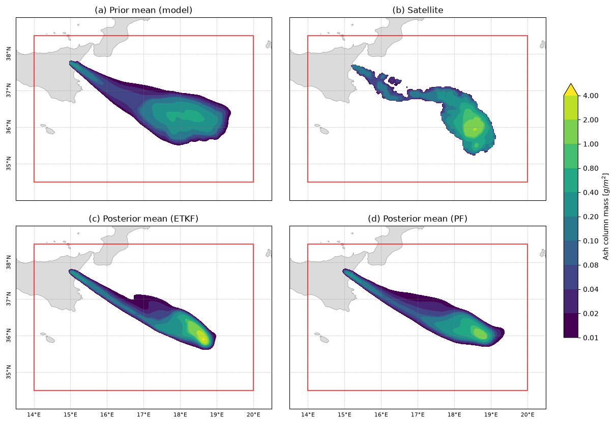
Figure 10 Spatial distribution of ash column mass at 18:00 UTC for the Etna 24 December 2018 case. (a) Ensemble mean of the model prior (128 members), (b) SEVIRI satellite retrieval, (c) ETKF posterior ensemble mean and, (d) PF posterior ensemble mean. The red box shows the extent of the FALL3D model domain.

5.3.1 VAE prior

The simulated model prior was used to train a new VAE used to generate an augmented ensemble (VAE prior) by sampling from the latent space. The same procedure and neural network architecture used for the synthetic experiments was also employed for the Etna experiment, with a few exceptions: (i) in order to accommodate the increased size of the input data, the latent dimension was increased from K=16 to K=32, and a new convolutional layer was added to both the encoder and decoder; (ii) we found that the chequerboard pattern could be reduced by replacing transposed convolutional upsampling by a bilinear interpolation and, (iii) rather than sampling the latent variables from a standard normal distribution, the latent vectors were sampled from a multivariate normal distribution,

$$\begin{array}{}\text{(24)}& {\mathbf{z}}_i\sim \mathcal{N}(\mathit{\mu },\mathbf{\Sigma }),\end{array}$$

where μ and Σ were estimated from the latent representations of the training ensemble. The VAE prior was then generated by sampling N_E=4096 latent vectors z_i from this distribution and then decoded to obtain the VAE prior in the original ash column mass space.

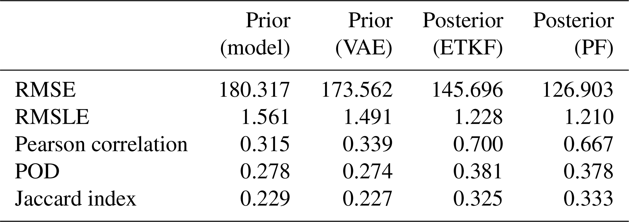
The agreement with the satellite observations was evaluated using the metrics defined in Sect. 4.5. Table 4 compares the model prior and VAE prior against the satellite retrievals. Metrics were computed for every ensemble member, and the ensemble average is reported in Table 4. Both model and VAE prior ensembles show very similar performance across all metrics, with the VAE prior yielding slightly better RMSE, RMSLE and Pearson correlation. These results indicate that the VAE-generated ensemble preserves the main characteristics of the model prior that are relevant to the comparison with observations. The results are also consistent with the previous experiment analysis, showing that the VAE can generate samples that are statistically comparable to those produced by the physics-based FALL3D model. These results provide a baseline for assessing the impact of DA in the next section, while also demonstrating that the VAE-generated ensemble provides a suitable prior for subsequent data assimilation experiments.

Table 4 Metrics used to quantify agreement with observations for the Etna data assimilation experiment.

5.3.2 Data assimilation experiments

The analysis ensemble means obtained with the ETKF (Fig. 10c) and PF (Fig. 10d) show that both intensity and location of the maximum are corrected with respect to the prior. However, the analysis ensembles retain the lack of representation of the veering and wind shear present in the prior, resulting in an almost unidirectional and less extended plume. This illustrates an obvious but important limitation of the assimilation: the analysis can preferentially select and combine ensemble members that are more consistent with the observations, but cannot recover spatial structures that are not represented in the prior ensemble.

The impact of the assimilation can be assessed in terms of the evaluation metrics reported in Table 4. These diagnostics are not intended as an independent validation, but rather to characterize the adjustment of the prior ensemble towards the observational constraints. The agreement with the observations improves for all metrics following assimilation. The RMSE is reduced by 16 % (ETKF) and 27 % (PF) relative to the VAE prior, while the RMSLE decreases by 18 % (ETKF) and 19 % (PF). The Pearson correlation approximately doubles for both methods. A larger relative improvement is obtained for the categorical metrics: the ETKF increases the POD and Jaccard index by 39 % and 43 %, respectively, while the corresponding increases for the PF are 38 % and 47 %. Overall, both assimilation approaches consistently adjust the ensemble towards the observations, with comparable performance across the different metrics considered.

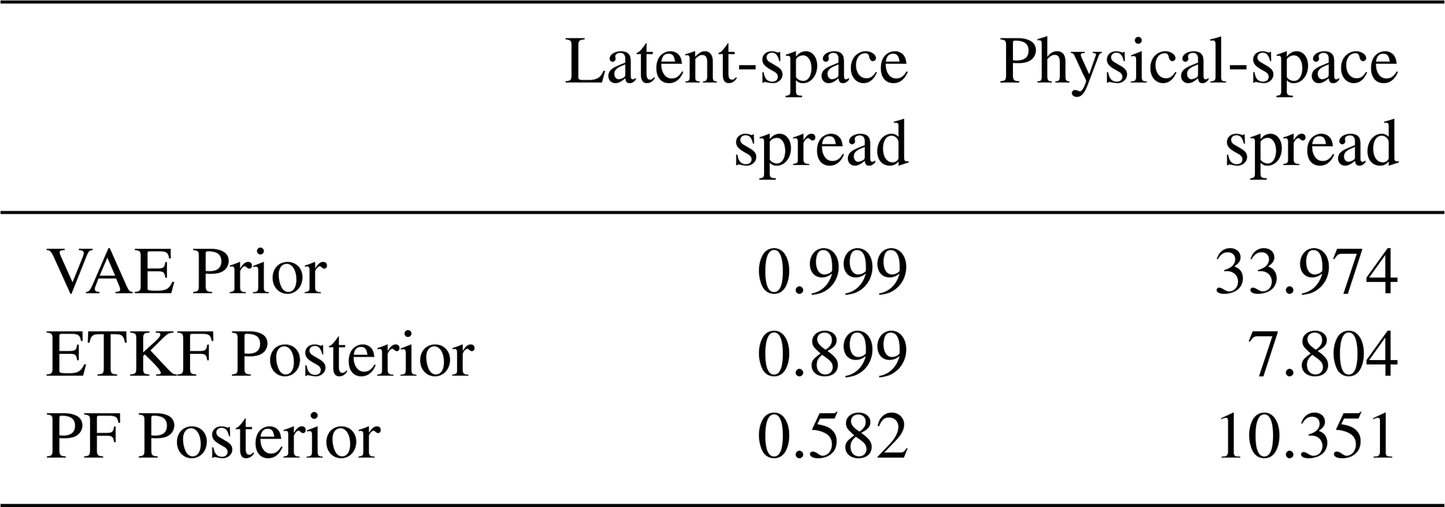
The impact of the assimilation can also be assessed in terms of the ensemble spread. The ensemble spread quantifies the dispersion of the ensemble members around the mean and is computed as the ensemble standard deviation at each element, averaged over all elements. The resulting spreads for the prior and posterior ensembles are reported in Table 5. This metric is evaluated both in physical space and in latent space. The spread reduction in latent space is 10 % (ETKF) and 42 % (PF). The substantially lower PF spread results from particle-filter degeneracy, with nearly all posterior probability concentrated on only two particles. Kernel perturbation is subsequently used to increase ensemble diversity, with a regularization factor of h=0.2 (see Sect. 3.3). Interestingly, the spread reduction in physical space is more pronounced for the ETKF (77 %) than for the PF (70 %), despite the substantially larger reduction observed for the PF in latent space.

Table 5 Ensemble spread of the prior and posterior ensembles in latent and physical space

The latent-space distributions of the prior and posterior ensembles are shown in Fig. 11 for selected pairs of latent dimensions, together with their corresponding histograms. In general, the prior distribution is well approximated by the standard normal distribution, as expected from the VAE construction. The ETKF produces a Gaussian-like posterior, whereas the PF analysis is clearly bimodal, reflecting the concentration of the posterior weights on two particles during the initial filter update. The subsequent kernel perturbation broadens these two modes, restoring some variability.

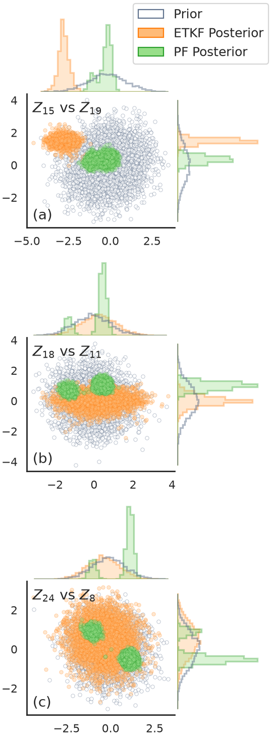
Figure 11 Latent-space distributions of the prior and posterior ensembles from the data assimilation experiments. Three selected pairs of the 32 latent dimensions are shown for illustration. The ensembles, each comprising 4096 members, are: VAE prior (white), ETKF posterior (orange), and PF posterior (green).

5.4 Discussion

In the context of this work, the VAE is viewed as a complement to the physics-based model. We showed that, making use of an ensemble of a few hundred simulations, the VAE can learn a compact, low-dimensional representation of the complex, high-dimensional variability captured by the physics-based simulations. This representation provides an alternative space in which the structure of the ensemble can be easily analysed and manipulated.

In this first work, the VAE is trained at a single forecast time to simplify the neural network architecture and avoid the need for additional layers for time encoding. This design choice reflects the complementary role of the VAE and the physics-based model: while the numerical model provides detailed temporal evolution of volcanic ash clouds, the VAE provides a robust statistical representation of the ensemble at the forecast times required for data assimilation or ensemble augmentation. By focusing on a single forecast time, the VAE can exploit the redundancy implicitly present in the ensemble of physics-based simulations to learn a low-dimensional manifold, while retaining a relatively simple and robust neural network architecture.

Sampling in the latent space to generate an augmented ensemble is the most straightforward application of this methodology. Although it does not introduce new physical knowledge, the VAE can generate a much larger number of realizations at very low computational cost during inference, while retaining variability that is statistically consistent with that captured by the physics-based simulations. It is interesting to consider whether this methodology can be computationally efficient, accounting for both training and inference, when generating ensembles much larger than the training ensemble. However, the answer is not simple as it depends on the available computational resources, the cost of the physics-based model, the total simulation time, and the ensemble size, among other factors. As an illustrative example, let's consider the Etna experiment, which is the most computationally demanding case presented here. The 128 FALL3D simulations were run on the accelerated partition of MareNostrum5 using 128 NVIDIA Hopper GPUs, requiring approximately 1 GPU-hour in total (i.e., aggregated across all GPUs). In contrast, VAE training was performed on a laptop using a single RTX 5000 Ada Generation NVIDIA GPU and required only 5.83 × 10⁻³ GPU-hours. In this experiment, the forecast period was limited to 8 h; extending the forecast period would further increase the relative cost of the numerical simulations. Most importantly, the approach substantially reduces the computational resources required to generate large ensembles; for example, the simulations for the synthetic experiment on the LUMI supercomputer required at least 2048 GPUs. Of course, these examples do not allow us to draw general conclusions about the relative efficiency of augmenting an ensemble with a VAE versus explicitly simulating larger ensembles, as the computational cost depends on the type of model and the available computational resources. However, computational efficiency is arguably not the main advantage of the proposed approach.

The methodology presented in this work also offers potential advantages beyond ensemble augmentation. Increasing the ensemble size can reduce sampling errors and improve the estimation of statistical quantities that are particularly sensitive to small ensemble sizes, such as exceedance probabilities and other measures of uncertainty. Such estimates are particularly relevant for probabilistic hazard assessment and decision-making in crisis management. For example, as shown in Sect. 5.2.2, the VAE provides a better approximation to the reference distribution than the training ensemble in terms of the Jensen–Shannon (JS) divergence when the ensemble size exceeds the number of numerical simulations used for training.

Additionally, due to the generative nature of the VAE, instead of simply duplicating or resampling existing numerical simulations, as in a bootstrap approach, new realizations absent from the original dataset can be generated. This could potentially lead to a richer statistical representation of the variability captured by the physics-based model, particularly if some of the generated realizations correspond to regions of the distribution that are poorly represented in the training ensemble. This interpretation is consistent with the results presented in Sect. 3, where the VAE-generated ensemble shows better agreement with the observations than the model prior in terms of RMSE, RMSLE, and Pearson correlation (Table 4).

Finally and most importantly, the learned representation enables different operations to be performed in a substantially lower-dimensional space, including data assimilation, clustering, perturbation, conditional sampling, and other statistical techniques. These capabilities provide an excellent opportunity for further research. In this study, we have explored two latent-space data assimilation approaches that, in the formulation adopted here, would not be directly applicable in the original physical space. The assimilation experiments demonstrate the feasibility of performing data assimilation directly in the VAE latent space. Both the ETKF and PF adjust the augmented prior towards the satellite observations, improving the agreement across all considered evaluation metrics and reducing the ensemble spread without an excessive loss of ensemble variability. Although the two assimilation approaches produce markedly different posterior distributions in latent space, their resulting posterior ensembles in physical space are relatively similar. The well-known particle-collapse problem of the PF was not fully resolved, as the posterior distribution remained concentrated around two particles, resulting in a bimodal distribution after the perturbation introduced by the kernel regularization. Applying such a naive perturbation directly in the physical space for a non-linear model would result in states that are inconsistent with the model dynamics. Instead, perturbing in latent space takes advantage of the learned mapping, allowing perturbed particles to be mapped back to physical space while retaining consistency with the physics-based simulations. This clearly illustrates one of the advantages of performing operations directly in the latent space.

Overall, the results presented in Sect. 5.3 demonstrate that latent-space data assimilation can effectively incorporate satellite observations to correct a large VAE-generated ensemble of two-dimensional volcanic ash column mass. Although the present study is centred on volcanic ash applications, the proposed methodology could be naturally extended to other atmospheric modelling and forecasting problems involving the transport and dispersion of atmospheric components. Potential applications include air-quality forecasting and, particularly, modelling of smoke transport from large wildfire events. Future research is needed to assess whether the methodology can be extended to the full three-dimensional concentration field and multiple particle classes, which will require adapting the neural network architecture to the increased dimensionality of the problem. This extension would be an important step for enabling multiple data assimilation cycles and, ultimately, supporting operational forecasting.

6 Conclusions

This study explored the potential of a hybrid strategy for volcanic-cloud modelling based on the integration of generative AI with physics-based simulations. A Variational Autoencoder (VAE) was trained on a relatively small ensemble of numerical simulations to learn a compact, low-dimensional representation of the high-dimensional problem. This methodology offers several potential advantages, including the generation of large ensembles at very low computational cost, the reduction of sampling errors and improved estimation of ensemble statistics, the generation of new samples beyond those contained in the training dataset, and the ability to perform statistical operations in a substantially lower-dimensional space, including latent-space data assimilation.

Two numerical experiments have been presented. A first synthetic experiment assessed the consistency of the VAE-generated ensemble using a controlled case characterized by multiple qualitatively different solutions, testing the ability of the VAE to capture this variability. Even when no new physical knowledge is introduced by a VAE-augmented ensemble, it provides a good statistical approximation of the reference distribution and generates fields that are statistically consistent with the underlying physical model, particularly at large spatial scales. The results also highlight limitations in the representation of smaller-scale spatial structures. However, the reconstruction error is smaller than the errors introduced by the numerical model itself. In the second experiment, the 24 December 2018 Etna eruption was modelled and the VAE-augmented ensemble was compared with satellite retrievals. The agreement with observations was found very similar for the numerical and VAE-augmented ensembles, with the latter yielding better RMSE, RMSLE, and Pearson correlation coefficients, suggesting that the generation of new samples can lead to a better statistical representation of forecast uncertainty. The Etna experiment was also used to provide a proof-of-concept demonstration of latent-space data assimilation methodologies. A two-dimensional estimation problem was solved by assimilating satellite retrievals in the VAE latent space. The analysis ensemble showed improved agreement with the observations across all evaluated metrics, while significantly reducing the ensemble spread and retaining the ability to represent the spatial variability of the volcanic cloud and the physical consistency with the simulated prior.

In summary, this work represents a first proof of concept based on a relatively simple neural architecture and an elementary data assimilation methodology. The results demonstrate the potential of the formulation, while highlighting the need for further research to assess its robustness and applicability across different eruption scenarios. Future work should extend the methodology to three-dimensional fields, explore more advanced generative models and assimilation approaches, and evaluate their performance against state-of-the-art DA methods and independent observations, ultimately assessing their potential implications for operational forecasting.