Correct use of radiative efficiencies in calculating global warming potentials and other emission metrics

The calculations of Global Warming Potentials (GWPs) and other related climate emission metrics should use radiative efficiencies that are calculated using the mean atmospheric mole fraction, rather than the surface mole fraction as is commonly used. We quantify this correction and show it leads to an upward revision of GWP values. For species with lifetimes greater than a few years, the revision is an increase of a few percent e.g., 7 % for trichlorofluoromethane (CFC-11). For species with lifetimes of the order of a year or less, this correction can lead to increases in the GWPs of over ten percent, which could impact on stakeholder decisions on the desirability of using such gases.

1 Introduction

The Global Warming Potential (GWP) of a species is given by the ratio of the absolute global warming potential (AGWP) to that of CO₂. The AGWPs are the radiative forcing following a 1 kg pulse emission integrated over a specified time horizon H with units of W m⁻² yr kg⁻¹ (e.g., Shine et al., 1990).

$$\begin{array}{}\text{(1)}& {\mathrm{AGWP}}_x=\underset{\mathrm{0}}{\overset{H}{\int }}{A}_x{R}_x\left(t\right)\mathrm{d}t\end{array}$$

Here A_x is the radiative forcing from 1 kg of species x (i.e. units of W m⁻² kg⁻¹), and R_x(t) is the time evolution of the atmospheric mass of the species following the pulse emission. Hence, the AGWPs are proportional to the radiative efficiency defined per unit mass of the emitted species.

Values of radiative efficiency for many species have been calculated (Etminan et al., 2016; Hodnebrog et al., 2020) but are usually reported defined per change in surface mole fraction. This letter sets out to clarify the importance of using the appropriate conversion from mole fraction to mass when calculating GWPs and other climate emission metrics.

2 Radiative efficiencies

The radiative efficiencies for atmospheric species are typically calculated using sophisticated radiative transfer models (RTMs) in which the mole fractions of the species of interest are varied. The radiative efficiencies are then calculated as the ratio of the radiative forcing change to the mole fraction change, for small changes in mole fraction. Originally calculations used constant profiles of mole fraction with height (e.g., Pinnock et al., 1995) but vertical profile information from models or observations was later adopted for many species (Etminan et al., 2016; Freckleton et al., 1998; Jain et al., 2000; Myhre et al., 1998; Myhre and Stordal, 1997; Naik et al., 2000). This is now done routinely in international assessments for halogenated gases using parameterisations based on species lifetime (Hodnebrog et al., 2013, 2020). These radiative efficiencies are typically reported per change in surface mole fraction (Etminan et al., 2016; Freckleton et al., 1998; Hodnebrog et al., 2013, 2020; Jain et al., 2000; Myhre et al., 1998; Myhre and Stordal, 1997; Naik et al., 2000) where “surface” refers to the perturbation imposed in the lowest layer in the RTM. Species that are destroyed in the stratosphere (N₂O, chlorofluorocarbons (CFCs)) will have lower mole fractions in the stratosphere than at the surface. Species that have very short tropospheric lifetimes (comparable to the vertical mixing timescales in the troposphere) such as some hydrocarbons and halocarbons will have significantly lower mole fractions in the upper troposphere than at the surface. In both cases the radiative forcing will be less (for the same surface mole fraction change) than if a constant profile were used, and so the radiative efficiency will be lower too. Figure 1a shows the adjustments to the radiative efficiency for species destroyed in the stratosphere (dashed red line) and troposphere (dashed blue line) based on parameterisations¹ derived in Hodnebrog et al. (2013). The adjustments can be considered to comprise two components, a correction due to the spatial distribution of the species (radiative efficiency per mass is greatest in the upper troposphere and lower stratosphere (Maycock et al., 2021) and over relatively cloud-free regions of higher surface temperature) and a correction because of the lower atmospheric mass of a species for a given surface mole fraction (solid lines in Fig. 1a).

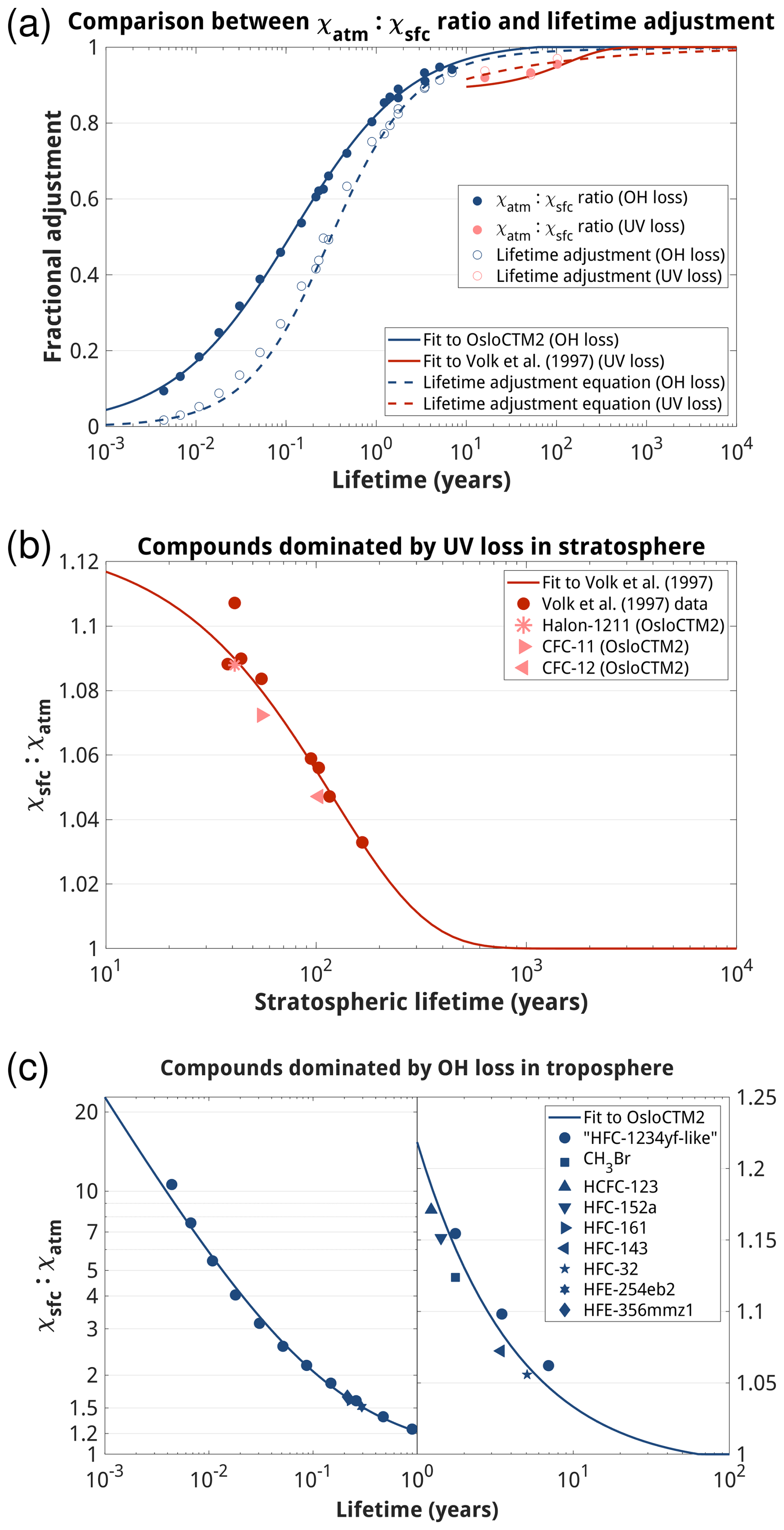
Figure 1 (a) Comparison between the ratio of mean atmospheric-to-surface mole fraction (χ_atm : χ_sfc; filled circles) and the lifetime adjustment that corrects RE to account for non-homogeneous atmospheric distribution (open circles) based on OsloCTM2 simulations (see Fig. 9 and associated discussion in Hodnebrog et al., 2013). (b) Ratio χ_sfc : χ_atm from the OsloCTM2 simulations, and from observations in Volk et al. (1997) and associated fit from Collins et al. (2026b) (see Eq. 4), against stratospheric lifetimes from WMO (2022). (c) Ratio χ_sfc : χ_atm against total lifetimes from OsloCTM2 simulations in Hodnebrog et al. (2013) and associated fit (see Eq. 5). Note that in (a), red filled circles and solid red line are plotted against stratospheric lifetimes and not total lifetimes.

A key use of radiative efficiencies is to determine the radiative forcing from observed changes in surface mole fractions of different species (Forster et al., 2021), although for species with a steep vertical gradient (lifetime < 1 year) the definitions of “surface” in the RTM may not correspond exactly to the definition of “surface” in the observations which are determined from measurements representative of the well-mixed lower troposphere (Gulev et al., 2021). Accounting for the declining mole fractions with height has allowed a more complete determination of their climate effects (Hodnebrog et al., 2013). These adjustments however make them less useful for directly determining GWPs which are based on radiative efficiency per mass. To calculate GWPs it is important to know what vertical profile has been used for the species in the radiation calculations so that the radiative efficiencies can be correctly converted to a mass basis.

3 Radiative forcing per mass

In the climate assessments from the Intergovernmental Panel on Climate Change (IPCC) and the ozone assessments from the World Meteorological Organization (WMO) (Forster et al., 2021; WMO, 2022), the conversion from mole fraction to mass has been done using the following formula (Aamaas et al., 2013; Shine et al., 2005)

$$\begin{array}{}\text{(2)}& A_x=\mathrm{RE}\times {\displaystyle \frac{M_{\mathrm{air}}}{M_x}}\times {\displaystyle \frac{{\mathrm{10}}^{\mathrm{9}}}{T_{\mathrm{M}}}}\end{array}$$

where A_x and RE are the radiative efficiencies given in W m⁻² kg⁻¹ and W m⁻² ppb⁻¹, respectively, M_air is the mean molecular weight of dry air (28.97 kg kmol⁻¹), M_x is the molecular weight of species x, and T_M is the total dry air mass of the atmosphere (5.1352 × 10¹⁸ kg; Trenberth and Smith, 2005). This conversion is appropriate if the RE is defined per mean atmospheric mole fraction change, but not if it is defined per surface mole fraction change since the assumed mass burden will be incorrect. In the latter case a correction factor $\frac{\mathrm{\Delta }{\mathit{\chi }}_{\mathrm{sfc}}}{\mathrm{\Delta }{\mathit{\chi }}_{\mathrm{atm}}}$ is needed (Collins et al., 2026b) that is the ratio of the change in surface mole fraction Δχ_sfc to the change in mass-weighted mean atmospheric mole fraction Δχ_atm, i.e. Eq. (2) should be modified to

$$\begin{array}{}\text{(3)}& A_x=\left(\mathrm{RE}\times {\displaystyle \frac{\mathrm{\Delta }{\mathit{\chi }}_{\mathrm{sfc}}}{\mathrm{\Delta }{\mathit{\chi }}_{\mathrm{atm}}}}\right)\times {\displaystyle \frac{M_{\mathrm{air}}}{M_x}}\times {\displaystyle \frac{{\mathrm{10}}^{\mathrm{9}}}{T_{\mathrm{M}}}}\end{array}$$

Physically, the radiative efficiency per mean atmospheric mole fraction (i.e. the whole term in parentheses in Eq. 3) is higher because a lower Δχ_atm (or equivalently a lower change in atmospheric burden) is required to generate the same forcing as a 1 ppb change in χ_sfc.

Ideally the ratio $\frac{{\mathit{\chi }}_{\mathrm{sfc}}}{{\mathit{\chi }}_{\mathrm{atm}}}$ should be that used in the original RTM calculations, but that is not available in all cases, so we fit empirical functions to allow values to be derived for any species. Values of $\frac{{\mathit{\chi }}_{\mathrm{sfc}}}{{\mathit{\chi }}_{\mathrm{atm}}}$ for a range of species were calculated in Volk et al. (1997). These were species where the main effect on the vertical profile came from destruction in the stratosphere. Collins et al. (2026b) derived the following empirical fit to the data in Volk et al. (1997):

$$\begin{array}{}\text{(4)}& {\displaystyle \frac{{\mathit{\chi }}_{\mathrm{sfc}}}{{\mathit{\chi }}_{\mathrm{atm}}}}={\displaystyle \frac{\mathrm{1}}{\mathrm{1}-\mathrm{0.113}{e}^{-\frac{{\mathit{\tau }}_{\mathrm{strat}}}{\mathrm{130}}}}}\end{array}$$

τ_strat is the stratospheric lifetime of a species in years (WMO, 2022). Note the reciprocal of this term $\left(\frac{{\mathit{\chi }}_{\mathrm{atm}}}{{\mathit{\chi }}_{\mathrm{sfc}}}\right)$ is similar to the “fill factor c” in Prather et al. (2012) although they use the tropospheric mole fraction in the denominator. Figure 1b shows that OsloCTM2 results from Hodnebrog et al. (2013) align well with the empirical fit that is based on Volk et al. (1997). The root mean squared error (RMSE) in the ratio using the fit is less than 0.008.

To calculate the $\frac{{\mathit{\chi }}_{\mathrm{sfc}}}{{\mathit{\chi }}_{\mathrm{atm}}}$ ratio for species with short tropospheric lifetimes we fit to OsloCTM2 results for a range of molecules that react with OH in the troposphere in Hodnebrog et al. (2013) using a similar form of equation to their lifetime adjustment (τ is the total atmospheric lifetime in years).

$$\begin{array}{}\text{(5)}& {\displaystyle \frac{{\mathit{\chi }}_{\mathrm{sfc}}}{{\mathit{\chi }}_{\mathrm{atm}}}}=\max \left({\displaystyle \frac{\mathrm{1}+\mathrm{3.908}{\mathit{\tau }}^{\mathrm{0.6512}}}{\mathrm{4.028}{\mathit{\tau }}^{\mathrm{0.648}}}},\mathrm{1}\right)\end{array}$$

Figure 1c shows this fit on top of the $\frac{{\mathit{\chi }}_{\mathrm{sfc}}}{{\mathit{\chi }}_{\mathrm{atm}}}$ ratio against lifetime for all the OsloCTM2 simulations. For species with a lifetime greater than 1 year (right hand panel of Fig. 1c) the RMSE in the ratio using the fit is less than 0.002. For species with a lifetime less than 1 year (left hand panel of Fig. 1c) we calculate a fractional uncertainty of 5 % of the ratio. For these species the mole fraction also varies horizontally in the radiative efficiency calculations so χ_sfc is the global mean mole fraction in the lowest model layer, both in the determination of radiative efficiency and in the fit in Fig. 1c. Equation (4) should be used for species where stratospheric loss through photolysis is more important (shorter stratospheric partial lifetime). Equation (5) should be used for species where loss through OH in the troposphere has the shorter partial lifetime.

Table 1 shows, for a few selected molecules, how correcting for the $\frac{{\mathit{\chi }}_{\mathrm{sfc}}}{{\mathit{\chi }}_{\mathrm{atm}}}$ impacts GWP100 values (i.e. for H=100 years). Although we use here GWP100 values from Forster et al. (2021) and WMO (2022) for illustration, the correction factors are appropriate for all climate metrics that use radiative efficiency at all timescales. For CFC-11 the increase is just over 7 %. For some shorter-lived HFCs the effect can be very large, suggesting the previous determinations of GWP100 were underestimated by over 10 %.

Table 1 The effect on GWP100 of correcting the approach for converting RE values from per ppb to per kg, compared to the previous approach, for a selection of molecules. For CH₄, N₂O, CFC-11, CFC-12 and Halon-1211 explicit correction factors are used as described in the text. For CFC-113 Eq. (4) is used, and Eq. (5) is used for the other halogenated compounds. Uncertainties arising from the use of the equations are provided for these species. Lifetimes, REs and AGWP${}_{{\mathrm{CO}}_{\mathrm{2}}}$ are as in WMO (2022) for the halogenated species, and in Forster et al. (2021) (We use here the GWP100 values from the Errata to the IPCC AR6 https://www.ipcc.ch/report/ar6/wg1/downloads/report/IPCC_AR6_WGI_Errata.pdf (last access: 1 September 2026) rather than from the tables initially published in Forster et al. (2021)) for CH₄ and N₂O. Note uncertainties in GWP100 are around 40 % for most of these species (Smith et al., 2021).

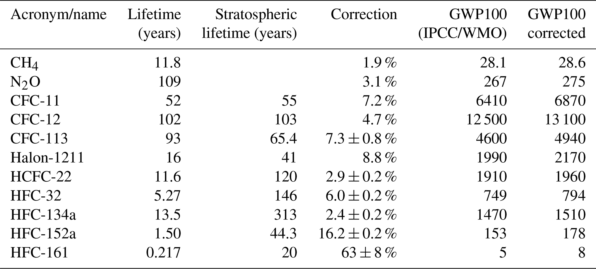
The methane and nitrous oxide radiative efficiencies used in the IPCC 6th Assessment (Forster et al., 2021) come from Etminan et al. (2016). The profiles of methane and nitrous oxide used in that study were from Myhre and Stordal (1997) (see Data Availability) with values of $\frac{{\mathit{\chi }}_{\mathrm{sfc}}}{{\mathit{\chi }}_{\mathrm{atm}}}$ of 1.019 and 1.031 respectively. Note these ratios are less than expected from Eq. (4). If the ratios used in the original radiative efficiency calculations are known, it is more appropriate to use these than Eqs. (4) or (5). In Hodnebrog et al. (2020) the explicit ratios for CFC-11, CFC-12 and Halon-1211 are 1.072, 1.047 and 1.088 respectively (Fig. 1b).

4 Discussion

The factor $\frac{\mathrm{\Delta }{\mathit{\chi }}_{\mathrm{sfc}}}{\mathrm{\Delta }{\mathit{\chi }}_{\mathrm{atm}}}$ discussed above is necessary to correct radiative efficiencies that have been reported per change in surface mole fraction when RE per change in mean atmospheric mole fraction is required, such as in the calculation of GWPs. This ratio should strictly be the ratio of the changes as used in the radiative efficiency calculations which is not necessarily that observed in the atmosphere or derived from models. Hence, we correct the methane and nitrous oxide radiative efficiencies using the profiles used in Etminan et al. (2016) rather than from Eq. (4). For CO₂, the radiative efficiency calculations from Etminan et al. (2016) and parameterised in Meinshausen et al. (2020) used a constant profile with height so do not need a correction. For halogenated species the ratios shown in Fig. 1c are taken from the profiles used to calculate the radiative efficiencies in Hodnebrog et al. (2013, 2020) so are appropriate to correct the reported values. For studies other than Etminan et al. (2016) and Hodnebrog et al. (2013, 2020) the $\frac{\mathrm{\Delta }{\mathit{\chi }}_{\mathrm{sfc}}}{\mathrm{\Delta }{\mathit{\chi }}_{\mathrm{atm}}}$ correction should ideally be taken from the profiles used in the RTM; however if these are not available our uncertainty analysis shows that Eqs. (4) and (5) are able to estimate the ratio to within less than 1 %. Although the GWP100 values for species with lifetimes less than a year are very uncertain and depend, for example, on where the species are emitted, they are widely reported and used; hence even for these it is important to correct systematic underestimates of over 10 %.

We have shown here the application to the GWP, but as most climate emission metrics (for example, GWP^* and global temperature-change potential – GTP) scale with the radiative efficiency per mass (e.g., Forster et al., 2021) these will be similarly affected, as will calculations of GWP for different time horizons.

However, calculations of radiative forcing from observed changes in surface mole fractions using radiative efficiencies should not use this correction. We recommend that, in future, calculations or assessments of radiative efficiencies report both the radiative forcing per surface mole fraction change and per mean-atmospheric mole fraction change.

5 Conclusions

We have shown that it is inconsistent to use radiative efficiency (per surface mole fraction) calculations in the standard GWP formulation if the radiative efficiency calculations account for decreases in atmospheric mole fraction above the surface. Since these calculations account for a decreased atmospheric mass of the species, this must also be accounted for in the conversion to radiative efficiency per mass; otherwise, the inconsistency will cause errors in the GWP calculation.

For species where the main decrease in mole fraction occurs in the stratosphere, the effect is only around 5 % to 7 % but, nevertheless, neglect of the correction leads to a systematic underestimate of the GWP. For species with short tropospheric lifetimes (of the order of a year or less) the underestimates can be 10 %, or even larger.

Correcting these underestimates could bring the GWP100 for some species over critical legislative thresholds (see, for example, Sect. 4 of Hodnebrog et al., 2020) and thus impact on their perceived desirability for use for certain applications. For instance, the GWP100 for HFC-32 increases from 749 to 794 (Table 1). It is recommended that the corrections provided in this letter are applied to GWP values and other climate emission metrics from the IPCC Assessment Reports and WMO Ozone Assessments.