Tropospheric oxidation chemistry and methane growth: a process-based attribution of OH variability (2003–2022)

Earth system models that include interactive chemistry provide a mechanistic understanding of the hydroxyl radical (OH) sources and sinks. However, their use is often limited in the estimation of the global methane (CH₄) budget. We conduct 20-year emission-driven methane simulations (2003–2022) with the Community Earth System Model Version 2.2 (CESM2.2) nudged to different meteorological datasets and input various chemical emissions dataset, including the Seventh Coupled Model Intercomparison Project (CMIP7). Our evaluation of the different model configurations includes comparison with in-situ observations from the NOAA Marine Boundary Layer Reference and airborne field studies, as well as ground-based and satellite remote sensing observations of carbon monoxide (CO) and CH₄. We find that the model configurations with a lower OH abundance have improved skill in reproducing both CO and CH₄ spatial and temporal variations, including the CH₄ annual growth rate. We quantify the OH impacts on the CH₄ growth rate and derive a comprehensive attribution of OH changes to Earth System chemical processes. Despite an interannual variability lower than 4 %, changes in OH explain around 30 % of the interannual variability of the CH₄ growth throughout the 2003–2022 period. The OH changes arise from both internal variability – via biogenic and lightning emission responses – and prescribed surface emissions. We find that OH is well buffered against chemistry perturbations, as increased chemical complexity raises the OH recycling probability. Consequently, studies relying on simplified and prescribed OH representations may neglect these complex chemical feedbacks and overestimate the role of OH changes in driving the CH₄ growth rate.

1 Introduction

Changes in atmospheric methane (CH₄) abundance depend on the balance between surface emissions and loss through microbial uptake in soils and atmospheric oxidation. Direct emissions from human activities such as fossil fuel production, agricultural activities such as livestock production and rice cultivation, and waste disposal, account for around 65 % of the total emissions (Saunois et al., 2025). The remaining sources are natural and are dominated by tropical and high latitude wetlands (e.g., Xiao et al., 2024), with minor contributions from fires, terrestrial permafrost, wild animals, termites, geological sources, as well as anthropogenic sources considered indirect, resulting from CH₄ emissions from water stagnating in dams and reservoirs. Given the large uncertainties and diversity of sources, the spatial and temporal variation of emissions are often estimated using Bayesian inverse models that combine prior flux estimates with CH₄ observations (e.g., Worden et al., 2023). Observational constraints on global methane budget include in-situ CH₄ mixing ratios and its isotopic ratio (¹³C:¹²C), denoted as δ¹³C-CH₄ (Lan et al., 2021a), its deuterium to hydrogen isotopic ratio (²H:¹H), denoted as δD-CH₄ (Riddell-Young et al., 2025), as well as satellite retrievals of atmospheric column concentrations (Jacob et al., 2022) such as the Greenhouse Gases Observing Satellite (GOSAT) launched in 2009 and the TROpospheric Monitoring Instrument (TROPOMI) since 2018.

Since 2000, changes in the atmospheric CH₄ growth rate have been characterized by a “pause” (1999 to 2006) of near-constant CH₄ atmospheric abundance, followed by “renewed growth” starting in 2007, with periods of “acceleration” when the global and annual CH₄ growth rate was higher than 10 ppb yr⁻¹ (Rigby et al., 2008; Dlugokencky et al., 2009; Nisbet et al., 2019, 2023; Nisbet and Manning, 2026). The inclusion of δ¹³C-CH₄ and δD-CH₄ measurements in flux inversions implies that the increase in microbial emissions explains most of the 2006–2022 increase in atmospheric CH₄ growth rate (Thompson et al., 2018; Basu et al., 2022; Michel et al., 2024; Riddell-Young et al., 2025; Oh et al., 2026; Yu et al., 2026). This is hypothesized to be driven by larger emissions from wetter and warmer tropical wetlands driven by precipitation and temperature increases during negative phases of the El Niño–Southern Oscillation (ENSO), i.e., La Niña years (Hodson et al., 2011; Zhu et al., 2017; Dean et al., 2018; Zhang et al., 2023). This is further corroborated by improved wetland carbon isotopic signature maps (Oh et al., 2022) and satellite-based inversions (Yin et al., 2021; Qu et al., 2024). Increases in farmed animals, waste management, and coal mining in China may have further contributed to the CH₄ rise since 2006 (Chandra et al., 2024). Recent studies indicate that the increase in CH₄ emissions during the 2019–2024 period is attributed to livestock, waste, and wetlands, dominated by sources in South America and Africa (He et al., 2026; Balasus et al., 2026). Yu et al. (2026) assimilated TROPOMI and CH₄ isotopologue observations and found a larger fossil fuel increase in China and a relative decrease of wetland CH₄ emissions from the Amazon Basin.

The hydroxyl radical •OH (hereafter denoted as OH for brevity) is the most important oxidant of the troposphere and thus controls atmospheric removal of many species including carbon monoxide (CO) and CH₄ (Levy, 1971). The primary source of OH is the reaction of water vapor (H₂O) with the excited oxygen atom O(¹D), produced by ozone (O₃) photolysis for wavelengths smaller than 330 nm:

$$\begin{array}{}\text{(R1)}& {\displaystyle }{\mathrm{O}}_{\mathrm{3}}+h\mathit{\upsilon }(\mathit{\lambda }<\mathrm{330}\mathrm{nm})\to \mathrm{O}{(}^{\mathrm{1}}\mathrm{D})+{\mathrm{O}}_{\mathrm{2}}\text{(R2)}& {\displaystyle }\mathrm{O}{(}^{\mathrm{1}}\mathrm{D})+{\mathrm{H}}_{\mathrm{2}}\mathrm{O}\to \mathrm{OH}+\mathrm{OH}\end{array}$$

As this reaction alone constitutes 50 % to 60 % of the OH sources, temperature, water vapor (expressed as specific humidity), and shortwave radiation reaching the troposphere (dependent on overhead O₃ in the stratosphere, driving O(¹D) production) are all important direct drivers of OH (e.g., Wang and Jacob, 1998; Holmes et al., 2013). The main OH losses are through its reaction with CO, CH₄ and isoprene in the lower troposphere across the tropics (Fiore et al., 2006; Lelieveld et al., 2016; Yoon et al., 2025). Early modeling studies suggested that large increases in CH₄ and, to a lesser extent, carbon monoxide (CO) during the second half of the 20th century could diminish the Earth's oxidation efficiency, defined as the globally averaged OH abundance (Crutzen and Zimmermann, 1991), if insufficient O₃ is produced during their oxidation (e.g., Logan et al., 1981). Thompson (1992) identified an increasing trend in tropospheric O₃ due to increases in precursor emissions, e.g., CH₄, CO, and non-methane hydrocarbons (NMHC). However, they could not easily identify OH trends due to the difficulty of balancing the concomitant increases in OH sources (O₃) and sinks (CO, CH₄).

The latest chemistry–climate model assessments, including AeroChemMIP as part of the Phase 6 of the Coupled Model Intercomparison Project (CMIP6), indicate that the rise in tropospheric O₃ since pre-industrial times is driven by increased anthropogenic sources rather than climate variability (Turnock et al., 2020; Griffiths et al., 2021; Fiore et al., 2022). Driven by economic activities, the increase in precursor emissions at lower latitudes of the Northern Hemisphere (NH), ongoing since the 1980s, has led to positive O₃ trends across the tropics, including the upper troposphere (Zhang et al., 2016; Yu et al., 2024; Froidevaux et al., 2025). As a result, chemistry–climate models tend to produce a net positive trend in OH since 1980 (Naik et al., 2013; Stevenson et al., 2020), driven by increasing O₃, nitrogen oxides (NO_x) and water vapor (Nicely et al., 2018; Chua et al., 2023), and decreasing anthropogenic CO emissions and abundance (Gaubert et al., 2017). Larger source of CH₄ contributes to the tropospheric O₃ growth and acts as a net sink for OH (Lelieveld et al., 1998; Shindell et al., 2005). Future OH abundance depends on which Shared Socioeconomic Pathway (SSP) emission scenario is used, where decreases in CO and CH₄ in the strong climate mitigation scenario (SSP1-2.6) are projected to reduce OH losses, increase OH, and thus further reduce the CH₄ lifetime (Liu et al., 2024). Staniaszek et al. (2022) performed simulations with a CH₄ emissions-driven version (Folberth et al., 2022) of the UK Earth System Model (UKESM1) and found that a hypothetical abatement of all CH₄ anthropogenic emissions caused a reduction in CO and hydroperoxyl radical (HO₂), slowing O₃ production and its role as OH source, yet still with increases in OH larger than 30 % due to the reduction of both CH₄ and CO. Aerosols, short-lived gases, and CH₄ act together to shape near-term climate and air quality. Allen et al. (2021) estimated that CH₄ mitigation could offset the warming induced by aerosol reductions while improving air quality.

While chemistry climate models simulate lower OH interannual variability (0.9 % to 1.8 % over 2000–2010, Saunois et al., 2025), observationally derived estimates suggest an interannual variability around 2 % to 3 % (e.g., Montzka et al., 2011; Patra et al., 2021; Yin et al., 2021). This contradiction has led to some skepticism about the use of global chemistry models to assess the role of OH in the CH₄ budget (Turner et al., 2019). However, methyl chloroform-based estimates are also subject to errors, in particular in two-box model inversions, allowing for both positive and negative OH trends within the uncertainty range (Rigby et al., 2017; Turner et al., 2017; Naus et al., 2019). As the declining atmospheric abundance of methyl chloroform reduces its ability to constrain OH for more recent periods, Thompson et al. (2024) used five hydrofluorocarbons as alternatives and found no significant OH trends, with a small interannual variability of less than 2 %. In contrast, Liu et al. (2025) estimated that from 1984 to 2020, the seasonal amplitude of atmospheric CH₄ increased from the northern mid-latitudes toward the Antarctic, a trend driven primarily by an enhanced CH₄ sink resulting from rising tropospheric OH abundance. Using Southern Hemisphere (SH) measurements of radiocarbon monoxide (¹⁴CO), a tracer produced by cosmic rays, Morgenstern et al. (2025) found a declining ¹⁴CO since 1997 at two remote locations, one in New Zealand and one in Antarctica. These two independent studies converge on the conclusion that OH has been increasing in the SH in recent decades. In this context, recent work has incorporated interannually varying OH fields, rather than climatological means (Patra et al., 2011), in light of the record-high CH₄ growth rate during the early 2020s (e.g., Chen et al., 2025; Zhao et al., 2025; Ciais et al., 2026). The inclusion of OH interannual variability and trends for other periods is acknowledged to have a significant impact on inverted emissions (e.g., Zhao et al., 2020; Belikov et al., 2026; Feng et al., 2026).

A more complete treatment of atmospheric chemistry is central to this effort. Improving this representation is key to CH₄ predictability within Earth system modelling frameworks (e.g., Folberth et al., 2025), and ultimately to Earth system predictability through a more complete understanding of the role of multi-scale chemistry processes as well as Earth system component interactions and feedbacks (Richter et al., 2026). Resolving the interaction across scales relevant for air quality and global trends would further support more accurate and efficient mitigation policy (Akimoto and Tanimoto, 2022). The inclusion of short-lived halogen (SLH) chemistry (e.g., Fernandez et al., 2026; Saiz-Lopez et al., 2025) has recently led to an important reduction in OH biases in the Community Earth System Model version 2.2 (CESM2.2), improving CH₄ prediction as well as CO in the NH during winter and spring (Mirrezaei et al., 2026a). The non-linear response of the CH₄-CO-OH chemical coupling alters how the CH₄ lifetime responds to an emission perturbation, which must be accurately represented to better quantify changes in CH₄ abundance. Notably, this inclusion of SLH chemistry reduced the global annual mean feedback factor (how much CH₄ lengthens its own atmospheric lifetime through its effect on OH) from 1.29 to 1.18, at the lower end of literature estimates (Szopa et al., 2021). However, it also highlights a positive feedback through the Cl‐driven oxidation pathways now quantified in SLH simulations and the total feedback factor including both Cl and OH is 1.34. More broadly, there is an urgent need to understand the interactions across spatial and temporal scales of the chemical fluxes involved in the sources and sinks of atmospheric oxidants, to reconcile modelled and observationally constrained estimates and to ultimately reduce uncertainties in OH across timescales (Szopa et al., 2021; Tan et al., 2026). Here, using a model with interactive chemistry, we identify and quantify the dynamical and chemical processes driving OH interannual variability and their impact on CH₄ growth rate, including previously overlooked anomalies. This allows us to assess the role of chemistry and CH₄ emissions in determining the atmospheric growth of CH₄.

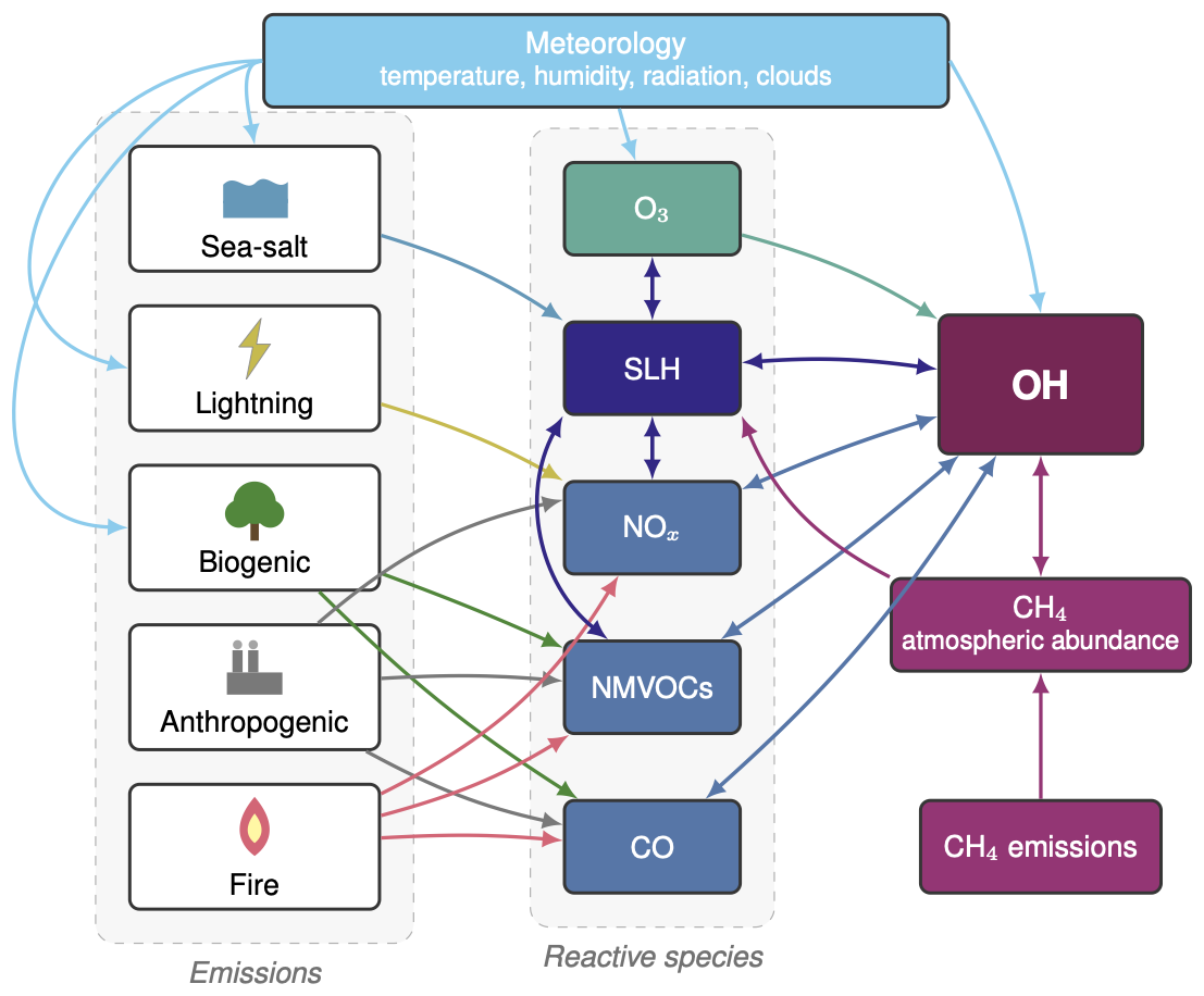
Figure 1 Schematic of the principal emission and chemical controls on tropospheric OH and their coupling to the methane budget. The chemical emission source categories (sea-salt aerosols, lightning, biogenic, anthropogenic, and fire) are displayed on the left and the main reactive species interacting with OH are in the middle row. Note that the model will include many interactions within the reactive species and OH and other species not shown here. Here we illustrate how SLH compounds are tightly coupled to various catalytic cycles. Meteorology (temperature, humidity, radiation, clouds) regulates photolysis rates, water vapor, and reaction kinetics, and additionally drives the biogenic, lightning sources and sea-salt sources interactively. On the right, CH₄ emissions show the source of atmospheric methane, while oxidation by OH provides its dominant atmospheric loss. The bidirectional coupling between CH₄ and OH indicates that changes in OH affect CH₄ abundance, while changes in CH₄ modify the OH sink. These interactions, together with SLH chemistry and the broader reactive chemical system (CO, NO_x, NMVOCs), regulate atmospheric oxidative capacity and CH₄ abundance.

Building on these recent model developments, we assess the role of meteorology and emissions in OH and CH₄ variability and trends using a set of emission-driven CH₄ simulations with CESM2.2. Specifically, we employ different sets of emissions of chemical species, including the newly released CMIP7 inventory, allowing us to contrast the role of anthropogenic and fire sources on the simulated tropospheric chemistry system. To evaluate the role of prescribed meteorological conditions, we also perform simulations with two different reanalysis datasets, the MERRA-2 (Modern-Era Retrospective analysis for Research and Applications, Version 2, Gelaro et al., 2017) and the fifth-generation ECMWF atmospheric reanalysis (ERA5, Hersbach et al., 2020). Figure 1 displays a simplified representation of the possible interactions and pathways impacting OH in our various simulations. The different meteorological forcings will impact directly the chemical species, or indirectly through changes in weather-driven emissions processes driving sea-salt, lightning and vegetation sources. Anthropogenic and fire emissions will impact non methane volatile organic compounds (NMVOCs), nitrogen oxides (NO and NO₂, NO_x), and CO. We present a thorough evaluation of the simulated CO and CH₄, as well as a detailed investigation of the chemical fluxes across these model configurations.

2 Methods

2.1 Community Atmosphere Model with chemistry (CAM-chem)

The open-source Community Earth System Model Version 2.2 (CESM2.2) is a modular software infrastructure that couples different components of the Earth System, i.e., the atmosphere, land and ocean (Danabasoglu et al., 2020). Based on the Community Atmosphere Model version 6 (CAM6), CAM-chem is the atmospheric component of the CESM2.2 with an interactive representation of physical, dynamical and chemical processes (Gettelman et al., 2019; Danabasoglu et al., 2020). The model has 32 vertical layers from the surface to around 40 km with a spatial resolution of 1.25° in longitude and 0.9° in latitude. Here we use the SLH chemistry presented in Fernandez et al. (2026) with the CH₄ emission-driven configuration described in Mirrezaei et al. (2026a), which includes updates to soil uptake of CH₄ and CO.

Table 1 Description of simulation experiments and input forcings. Presc. stands for CMIP6 prescribed CH₄ experiment, with SSP scenarios after 2015. CT-CH4-2025 means (NOAA CarbonTracker-CH4 2025, Oh et al., 2025). The MOPITT inversions are the results from Gaubert et al. (2024). CEDS-CMIP refers to CEDS-CMIP-2025-04-18 and CAMS-MOSAIC refers to CAMS-GLOB-ANT_m1.1. FINN2.5 refers to the Fire INventory from NCAR version 2.5 (Wiedinmyer et al., 2023), and BB4CMIP7-2-1 refers to the biomass-burning emissions dataset prepared for CMIP7 (BB4CMIP7, version 2-1). CEDS-CMIPx1.3 denotes the CEDS-CMIP anthropogenic CO emissions scaled by a factor of 1.3 (a 30 % increase).

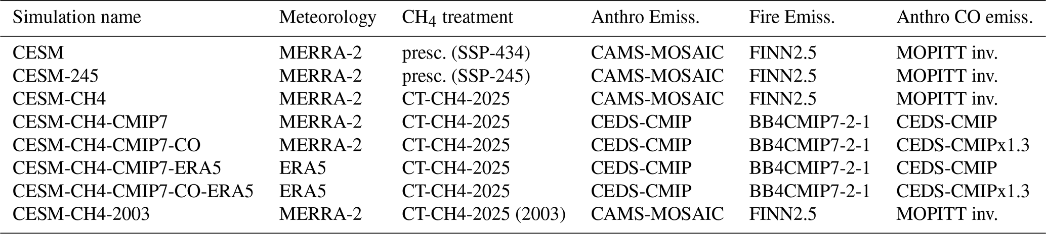
Table 1 lists the simulations conducted in this study. Our baseline simulation (CESM) uses the CMIP6 prescription of surface greenhouse gases (Meinshausen et al., 2017), extended with the Shared Socioeconomic Pathways 4-34 (SSP434) after 2015, with an alternative run (CESM-245) using the SSP245 to look at a different prescribed CH₄ distribution. The two scenarios do not differ widely for the considered period (2015–2022). Aside from the CESM-245 that is branched on 1 January 2015 from the baseline simulation (CESM), all the simulations are initialized from a previous CAM-chem concentration-driven simulation's initial conditions on 1 January 2002 and we use the year 2002 as the spin-up. All the CH₄ emission-driven simulations input posterior CH₄ fluxes from the NOAA CarbonTracker-CH4 2025 (CT-CH4-2025, Oh et al., 2025). For other chemical emissions, the CESM-CH4 uses the CAMS-GLOB-ANT_m1.1 (denoted hereafter as CAMS-MOSAIC) anthropogenic emission fluxes which include corrections based on national inventories in Europe, the USA and China with corrections at the state or province levels (Granier et al., 2025; Bouarar et al., 2026). However, surface CO anthropogenic fluxes are replaced with the posterior CO emissions from Gaubert et al. (2024). In a previous study (Mirrezaei et al., 2026a), we found that higher emissions in the NH were reducing OH biases and providing a better fit to CO and CH₄ observations. Wildfire emissions of chemical species other than CH₄ are prescribed from the Fire INventory from NCAR version 2.5 (Wiedinmyer et al., 2023), hereafter FINNv2.5. The CESM-CH4-CMIP7 uses the new set of emissions prepared for phase 7 of the CMIP, which consists of Community Emissions Data System (CEDS) released on 18 April 2025 (CEDS-CMIP-2025-04-18) for anthropogenic emissions (Hoesly et al., 2018; Feng et al., 2020; Hoesly et al., 2025) and the BB4CMIP7-2-1 fire emissions (van Marle and van der Werf, 2025). During our study period, the CMIP7 monthly wildfire emissions are derived from the Global Fire Emissions Database version 4.1s (Randerson et al., 2015; van Marle et al., 2017).

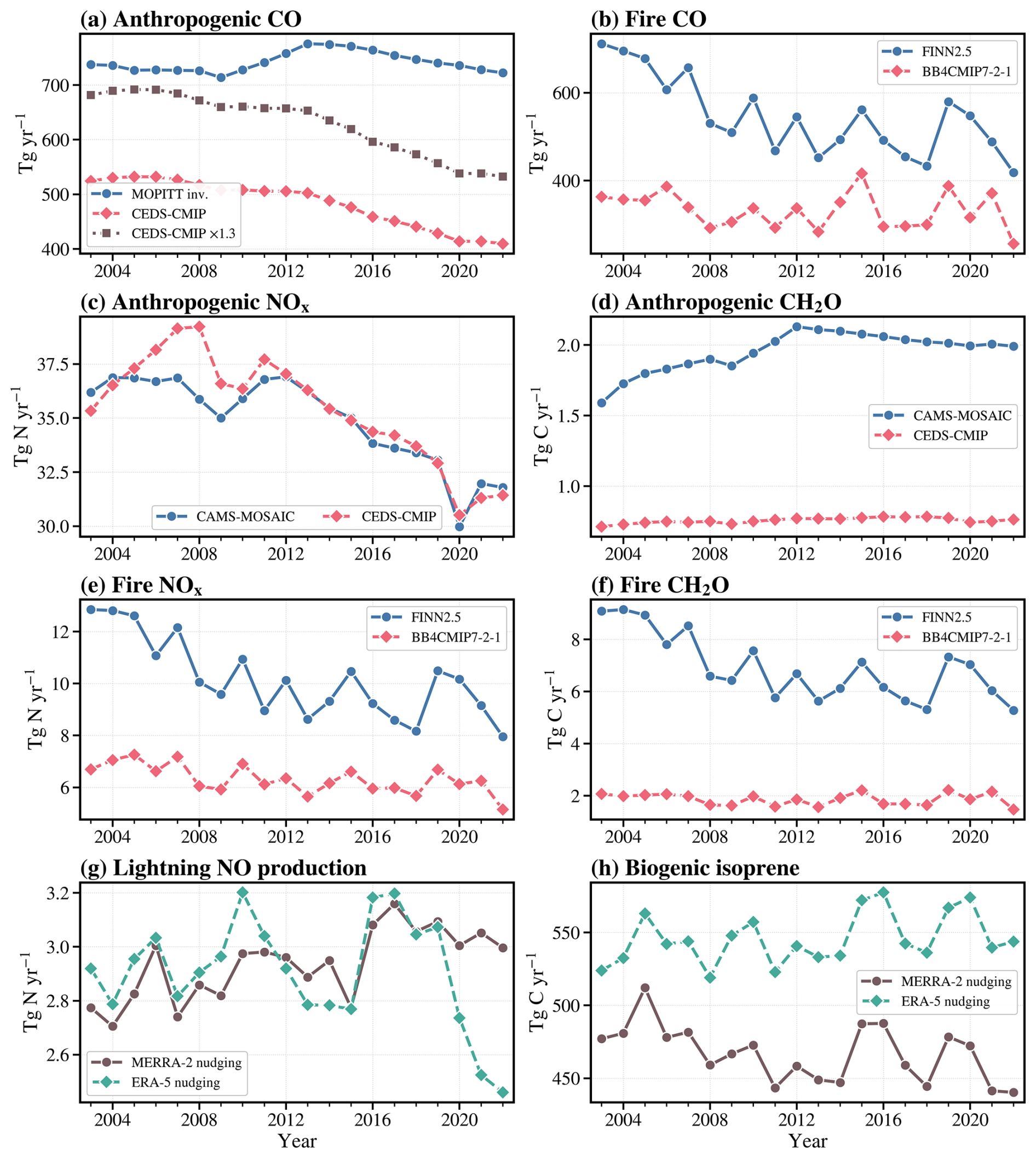
Figure 2 Global and annual emissions for (a) Anthropogenic CO, (b) Fire CO, (c) Anthropogenic surface NO_x, (d) Anthropogenic surface CH₂O, (e) Fire surface NO_x, (f) Fire surface HCHO, (g) NO_x from lightning, (h) Biogenic isoprene.

Figure 2 displays the emission time series estimated by the different datasets used in this study. With anthropogenic totals higher than 700 Tg CO yr⁻¹, the posterior CO emissions are much larger than the CEDS-CMIP7, which ranges between 400 and 500 Tg CO yr⁻¹. By construction, the posterior CO replicates the temporal variations from the prior CAMS-GLOB-ANT v5.3 inventory (Soulie et al., 2024), with no apparent trend globally. In contrast, the CEDS-CMIP7 shows a reduction of around 20 %, which likely is closer to observational estimates of 14 %–17 % reduction (approximately 85–110 Tg yr⁻¹) from Tang et al. (2026). Because of the differences in anthropogenic emissions, we also perform another simulation with anthropogenic CO increased by 30 % for the entire period (CESM-CH4-CMIP7-CO).

At every physical time step (30 min) and for all vertical levels, winds, temperature as well as specific humidity (Mirrezaei et al., 2026a) are nudged to the MERRA-2 (Gelaro et al., 2017) using the 3-hourly outputs with a relaxation time of 12 h (Davis et al., 2022). We also performed a couple of simulations with CMIP7 forcings (CESM-CH4-CMIP7-ERA5 and CESM-CH4-CMIP7-CO-ERA5) nudged to ERA5 hourly outputs (Hersbach et al., 2020). The ERA5 nudging is applied to the same variables and the same nudging strength as the MERRA-2.

In CESM, NMVOCs emissions from vegetation are estimated interactively in the Community Land Model (CLM) by the Model of Emission of Gases and Aerosols from Nature (MEGANv2.1), as initially described in Guenther et al. (2012). Thus, different atmospheric conditions can have strong impacts on biogenic emissions even though the phenology (parametrized by leaf area index) is prescribed by a climatology in our simulations. The monthly global isoprene emissions are reported in Fig. 2 and show an offset between the two used reanalysis with a 2003–2022 average of 466 Tg C yr⁻¹ (MERRA-2) and 545 Tg C yr⁻¹ (ERA5). We found that the ERA5-nudged simulation is warmer over the tropical continents where isoprene emissions are higher (Fig. S1 iin the Supplement), suggesting that the temperature is driving emission change. Our isoprene emission estimates are higher than a recent TROPOMI inversion (Sfendla et al., 2026) and of the CAMS-GLOB-BIOv3.1 dataset, who estimated isoprene emissions to be 389 Tg C yr⁻¹ for 2000–2019 (Sindelarova et al., 2022). However, they are well within the range of the most recent studies that derived isoprene emissions using Cross‐track infrared sounder (CrIS) isoprene retrievals, with 456 ± 238 Tg C yr⁻¹ over 2013–2020 period (Li et al., 2025) and 628–711 Tg C yr⁻¹ for 2019–2020 (Yoon et al., 2025).

Our lightning totals are around 3 Tg N yr⁻¹, which is in accordance with a recent estimate of 3.2 Tg N yr⁻¹ by Dang et al. (2026) and are on the lower end of the range 5 ± 2 Tg N yr⁻¹ from the recent literature review by Pickering et al. (2026).

2.2 Airborne Field Campaign Observations

We evaluate the simulations with four different field campaign observations. First, the High-Performance Instrumented Airborne Platform for Environmental Research (HIAPER) Pole-to-Pole Observations (HIPPO) aircraft campaigns (Wofsy, 2011) consisted of five deployments of the NSF/NCAR Gulfstream V aircraft (GV) in different seasons during the 2009–2011 period. The airborne vertical profiles provide CO and CH₄ in-situ measurements along the Pacific ocean between 87° N and 67° S (Santoni et al., 2014; Gaubert et al., 2019). Second, the NASA Atmospheric Tomography Mission (ATom) also provides a global survey of atmospheric composition with CO and CH₄ measured by the NOAA Picarro instrument (McKain and Sweeney, 2021). With hundreds of vertical profiles, ATom provides a global survey of the remote environment providing cross-sections along north-south gradients of the Atlantic and the Pacific Ocean for 4 different deployments during the 2016–2018 period (Thompson et al., 2022). Third, we compare the results for O₃, CH₄ and CO with the Korea–United States Air Quality (KORUS-AQ) field study (Crawford et al., 2021). The KORUS-AQ experiment occurred in May and June 2016 and was characterized by high O₃ and CO pollution resulting from both local sources and long-range transport of East Asian sources (Miyazaki et al., 2019; Gaubert et al., 2020). Last, the Asian summer monsoon Chemical and Climate Impact Project (ACCLIP) occurred in August 2022 (Pan et al., 2024) and thus provides a snapshot of the conditions at the end of the study period. We use observations made aboard the NSF/NCAR GV which sampled a quite large area of the Western Pacific around South Korea and Japan, with flight durations of around 8 h. All the in-situ CO observations used in this study were calibrated on the WMO CO X2014A scale and the CH₄ measurements WMO CH4 X2004A standard.

2.3 NOAA Marine Boundary Layer Reference

We compared our simulations to the global and zonal means of CH₄ from NOAA Greenhouse Gas Marine Boundary Layer Reference (Lan et al., 2024) which is derived from a subset of CH₄ measurements from air samples that are predominantly of well-mixed marine boundary layer (MBL) air with data smoothing and averaging approach from Masarie and Tans (1995). We linearly interpolate the 3-hourly model outputs in space and time to the observation locations and process the data in the same way as the MBL Reference.

2.4 Network for the Detection of Atmospheric Composition Change FTIR CO and CH₄ column retrievals

Ground-based Fourier Transform Infrared (FTIR) spectrometers operated within the Network for the Detection of Atmospheric Composition Change (NDACC) are used to further evaluate model simulations (De Mazière et al., 2018). The NDACC FTIR network spans a wide range of environments, from remote regions to sites influenced by urban emissions, providing broad geographic coverage for model evaluation. These instruments acquire direct-sun spectra under cloud-free conditions in selected mid-infrared spectral regions at a nominal spectral resolution of 0.004 cm⁻¹, enabling the retrieval of total columns and vertical information for CO, CH₄, and other atmospheric trace gases. NDACC FTIR observations are particularly well suited for investigating atmospheric variability and long-term trends. In this study, measurements from 21 NDACC sites were obtained from the NDACC archive (https://ndacc.larc.nasa.gov/, last access: 4 November 2026) and daily mean total columns were calculated for dates coincident with the model simulations. The current analysis uses products generated with the retrieval strategies presently available in the archive. While these products are suitable for total-column comparisons, future analyses will incorporate updated retrievals that provide improved tropospheric and stratospheric information (Ortega et al., 2025). To ensure a consistent comparison, modelled vertical profiles were smoothed using the FTIR averaging kernels and a priori profiles, thereby accounting for the instrument's vertical sensitivity. The resulting smoothed model columns were then compared directly with the FTIR columns.

2.5 Measurements of Pollution in the Troposphere (MOPITT) CO column retrievals

The MOPITT instrument (Drummond et al., 2010) measures CO absorption bands in the near infrared (NIR, λ=2.3 µm) and the thermal infrared (TIR, λ=4.7 µm). The version 9 (V9J) of the joint retrievals (Worden et al., 2010) estimates CO from both NIR and TIR and is described in Deeter et al. (2022). We use the level 3 product, which consists of monthly mean CO on a 1°×1° grid and is expressed here as column-averaged dry-air mole fraction. We apply the column forward operator to the regridded monthly model outputs.

2.6 Greenhouse Gases Observing Satellite (GOSAT) CH₄ column retrievals

We additionally evaluate the simulated column CH₄ against the University of Leicester GOSAT Proxy v9.0 product (Parker et al., 2020), retrieved from shortwave-infrared radiances measured by the JAXA Greenhouse Gases Observing Satellite (Kuze et al., 2009). Each Level-2 data, with its prior profile, pressure weights and column averaging kernel, is mapped to the CAM-chem grid (0.9°×1.25°). The simulated CH₄ is then interpolated onto the 20 retrieval levels and smoothed with the retrieval prior and averaging kernels following Appendix D of Parker and Boesch (2020). Following Balasus et al. (2023), we reduced the GOSAT retrievals by 9.2 ppb to align them with the reference used by the blended TROPOMI+GOSAT product, which is also used for comparison.

2.7 TROpospheric Monitoring Instrument (TROPOMI) CO and CH₄ column retrievals

Flying on the ESA Copernicus Sentinel-5 Precursor platform, the TROPOMI instrument (Veefkind et al., 2012) is an imaging spectrometer passively measuring the reflected solar radiation, from which the column-averaged dry-air mole fraction of methane (XCH₄) can be estimated in the 1.65 µm band. For XCH₄ from TROPOMI we use the blended TROPOMI+GOSAT product of Balasus et al. (2023), in which the operational retrieval (Lorente et al., 2021) is recalibrated against GOSAT to remove albedo and aerosol related biases. The level-2 data are regridded to the CAM-chem resolution and the column averaging kernels are applied to the model profile. For CO, we use the Sentinel-5P TROPOMI CO total-column product (Borsdorff et al., 2018; Martínez-Alonso et al., 2020). We apply surface-dependent quality filtering, with only the highest-quality pixels over land (qa =1.0), and only pixels with qa ≥0.7 over ocean (excluding coastlines, lakes and inland water). Following Inness et al. (2022), the total-column averaging kernel is applied directly to the co-sampled model profile.

3 Results

3.1 Evaluation with Airborne Field Campaign Observations

Since the simulation results are quite consistent despite covering different regions and periods, we aggregate the comparison for the 4 different field campaigns in Fig. 3. First, the CESM-SSP245 simulation, with prescribed CH₄ from observations before 2015 and SSP245 afterward, has the lowest CH₄ bias compared to campaign observations from remote regions, i.e., HIPPO and ATom. During KORUS-AQ and ACCLIP, these concentration-driven simulations lack vertical variability in the model, resulting from the prescription of zonally averaged concentration fields that smear the gradients in these regions where regional emissions dominate. The model shows a low CH₄ bias during KORUS-AQ with both CESM-SSP245 and CESM-SSP434, but not during ACCLIP where the CESM-SSP245 simulates CH₄ quite well. This shows the difficulty of capturing the large temporal variations in CH₄ with the assumed emission/concentration projections in SSPs. Second, the CESM-CH4 simulation, with emission-driven CH₄, CAMS-MOSAIC, posterior CO, and FINN2.5 for chemical emissions provides better results for CH₄, CO and O₃, consistently across all field campaigns. The simulation has improved CH₄ vertical gradients and sometimes a lower bias than the prescribed CH₄ simulations. The boundary layer profile is correctly simulated by the CESM-CH4 simulation while the free tropospheric CH₄ is slightly underestimated, indicative of an overall OH overestimation, or an underestimation of the CH₄ sources during ACCLIP in summer 2022. Third, despite having the same CH₄ emissions, the set of simulations with emissions from CMIP7 (CESM-CH4-CMIP7 and CESM-CH4-CMIP7-CO) has a much lower CH₄ compared with the observations. The increase in CO (CESM-CH4-CMIP7-CO) only partially mitigates the CO underestimation and, through an OH reduction, the CH₄ low biases. Fourth, the simulations with nudging to ERA5 show a much lower CH₄ and CO bias, indicative of a lower OH driven by meteorological differences (everything else being equal). The CESM-CH4-CMIP7-CO-ERA5 has a lower CH₄ underestimation and its profiles are closer to the CESM-CH4 simulation for both CH₄ and CO. This means the OH is lower in the CESM-CH4-CMIP7-CO-ERA5.

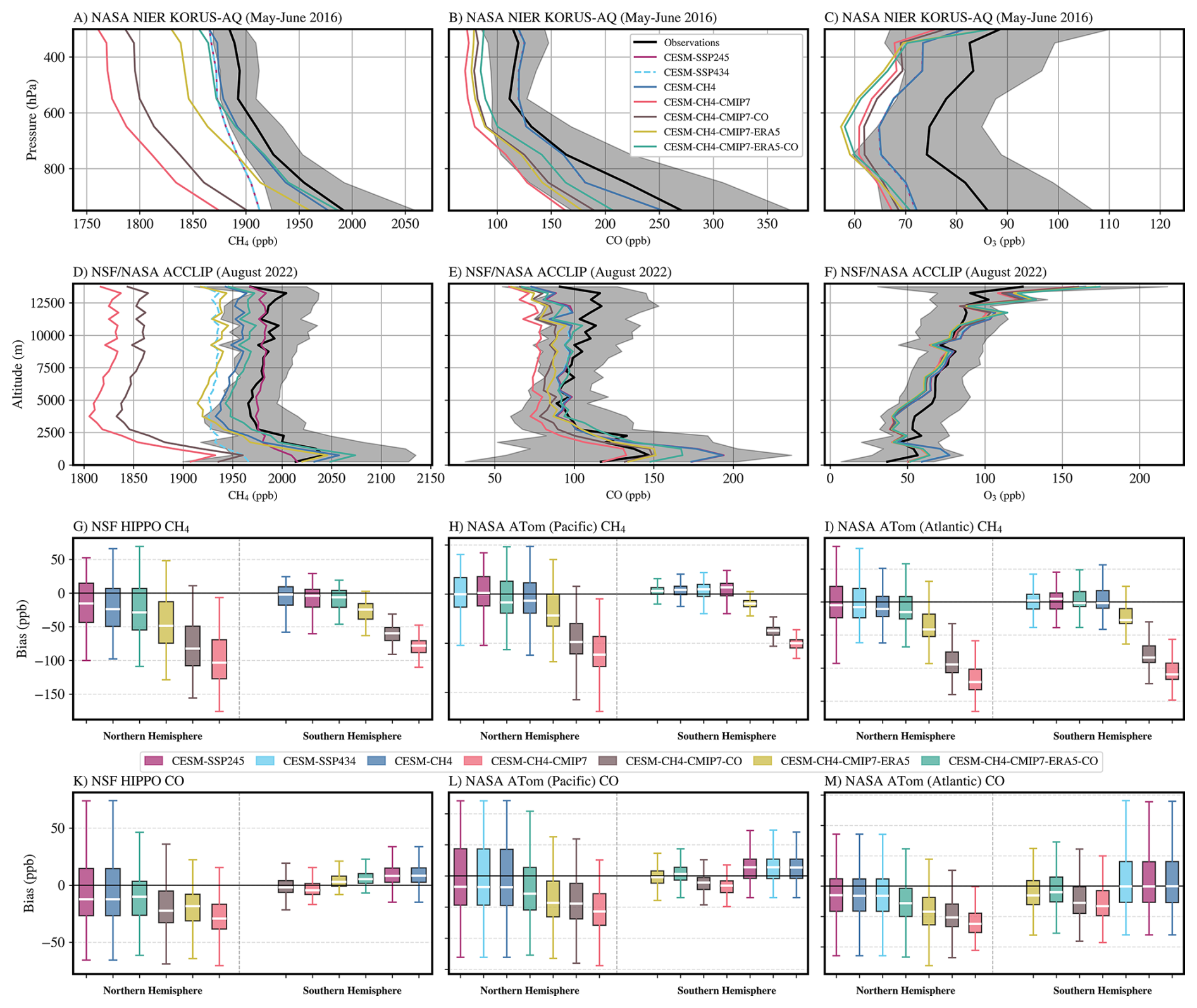
Figure 3 Comparison of simulation and observations of NIER/NASA KORUS-AQ for (A) CH₄, (B) CO and (C) O₃ and with NSF/NASA ACCLIP for (D) CH₄, (E) CO and (F) O₃. The grey area represents the observations standard deviation within each altitude bins (100 hPa for KORUS-AQ and 500 m for ACCLIP). The distribution of the bias for NSF HIPPO and NASA ATom are shown by hemisphere for CH₄ (G, H, I) and CO (K, L, M).

Regarding CO, the simulations using the posterior emissions overestimate the observations in the boundary layer around the Seoul Metropolitan Area during ACCLIP but the free tropospheric abundance is quite well simulated. Conversely, the CESM-CH4-CMIP7 with smaller CO emission reproduces the boundary layer CO but underestimates the East-Asian background, probably because of a combination of an OH overestimation and/or an underestimation of the CO sources in East Asia. This might explain the O₃ overestimation in the boundary layer seen in CESM-CH4 but not in CESM-CH4-CMIP7. Overall, this set of experiments shows that simulated CO tends to be underestimated in the NH in all the experiments with CMIP7 forcings. This could be the results of an indirect effect through a lack of NMVOCs emissions consuming OH and potentially producing CO in the atmosphere or the direct CO emission underestimation (that motivates our COX1.3 experiment), but it is likely a combination of both. However, as anthropogenic CO emissions are being reduced over the recent years, simulations with CMIP7 emissions provides a better CO during ACCLIP (summer 2022) than during KORUS-AQ (spring 2016), indicative of a better representation of the declining trends in CMIP7 than the posterior emissions derived from the weak trend of CAMS-GLOB-ANTv5.1. Finally, simulations run with the FINN2.5 emissions tend to overestimate CO in the SH, related to the much higher estimate of fire CO emission compared to BB4CMIP7.

3.2 Evaluation against remote sensing observations

Figure 4 presents the summary comparison of simulated CO and CH₄ with TROPOMI, NDACC, GOSAT and MOPITT observations. The NDACC network has less coverage but higher spectral resolution and is used as reference for the given period (January 2010 to December 2021 for GOSAT and May 2018 to December 2022 for TROPOMI). In line with the in-situ aircraft field campaign observations comparison, the remote sensing observations show that the CESM-CH4 and CESM-CH4-CMIP7-CO-ERA5 perform best in simulating CH₄. These are the only two simulations with biases lower than 1 % for GOSAT, TROPOMI, and NDACC for both periods. The CESM-CH4-CMIP7 and the CESM-CH4-CMIP7-CO have a systematic bias of around 4 % to 6 % and indicate a reduction of up to 1 % in CH₄ low bias with an increase of anthropogenic CO by 30 %. The CH₄ bias is reduced by 5 % between CESM-CH4-CMIP7-ERA5 and CESM-CH4-CMIP7. Thereofore, the CESM-CH4-CMIP7-ERA5 has low biases, but underestimates CH₄ more than CESM-CH4 during the GOSAT period. The random error (the unbiased RMSE, uRMSE) component does not vary as much as the systematic error across the experiments.

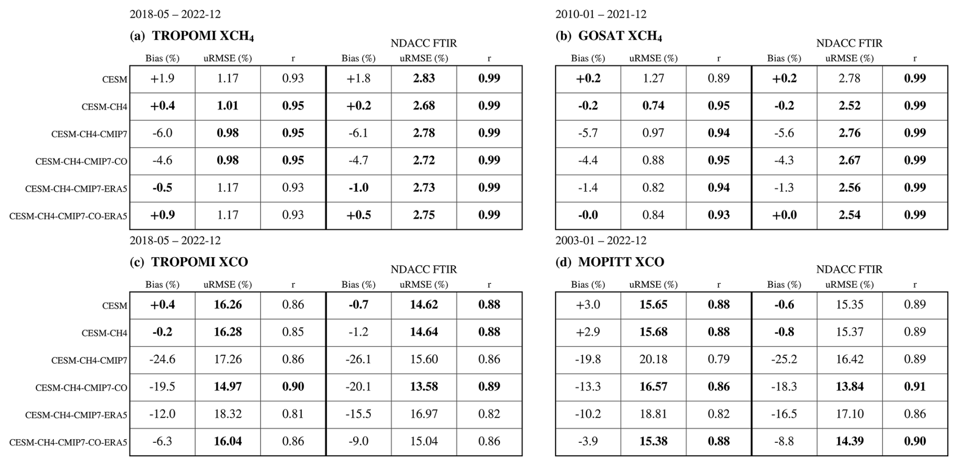
Figure 4 Comparison of simulation and observations for various periods and datasets: (A) May 2018–December 2022 TROPOMI XCH4 (n=1 191 664) and NDACC XCH4 (n=7237), (B) January 2010–December 2021 GOSAT XCH4 (n=801 568) and NDACC XCH4 (n=19 052), (C) May 2018–December 2022 TROPOMI XCO (n=2 449 501) and NDACC XCO (n=7157), and (D) January 2003–December 2022, MOPITT (n=12 063 679) and NDACC XCO (n=26 921). The bias is shown on a diverging blue–white–red scale (blue where the model is lower than the observations, red where it is higher and white near zero), so colour shows both the sign and the magnitude of the bias. The unbiased RMSE (uRMSE) and the correlation coefficient r use sequential scales in which green marks the better value (low uRMSE, high r) and red/pale yellow the poorer value. Within each species (CH₄: A, B; CO: C, D), each metric (bias, uRMSE, and r) uses a single colour scale shared across both panels and across the satellite and NDACC FTIR blocks. For each dataset, the mean bias (systematic error, %), the unbiased RMSE (uRMSE, random error, %) and the correlation coefficient r are given.

The relative uncertainties are higher for CO than for CH₄. Simulations that use the posterior CO emissions estimated by Gaubert et al. (2024) have no biases on average with regard to TROPOMI, i.e., for the most recent period, and a small overestimation compared to MOPITT with errors of less than 3 %. Simulations with the setup following the CMIP7 protocols have a low CO compared to TROPOMI, MOPITT and NDACC observations, with up to a 25 % underestimation for CESM-CH4-CMIP7. Increasing the anthropogenic CO emissions by 30 % reduces both the systematic and random errors, with around 5 % reduction in biases for all the observing systems. Consistent with the in-situ evaluation, replacing MERRA-2 with ERA5 substantially improved the performance of CESM-CH4-CMIP7-CO-ERA5 relative to CESM-CH4-CMIP7-CO simulation.

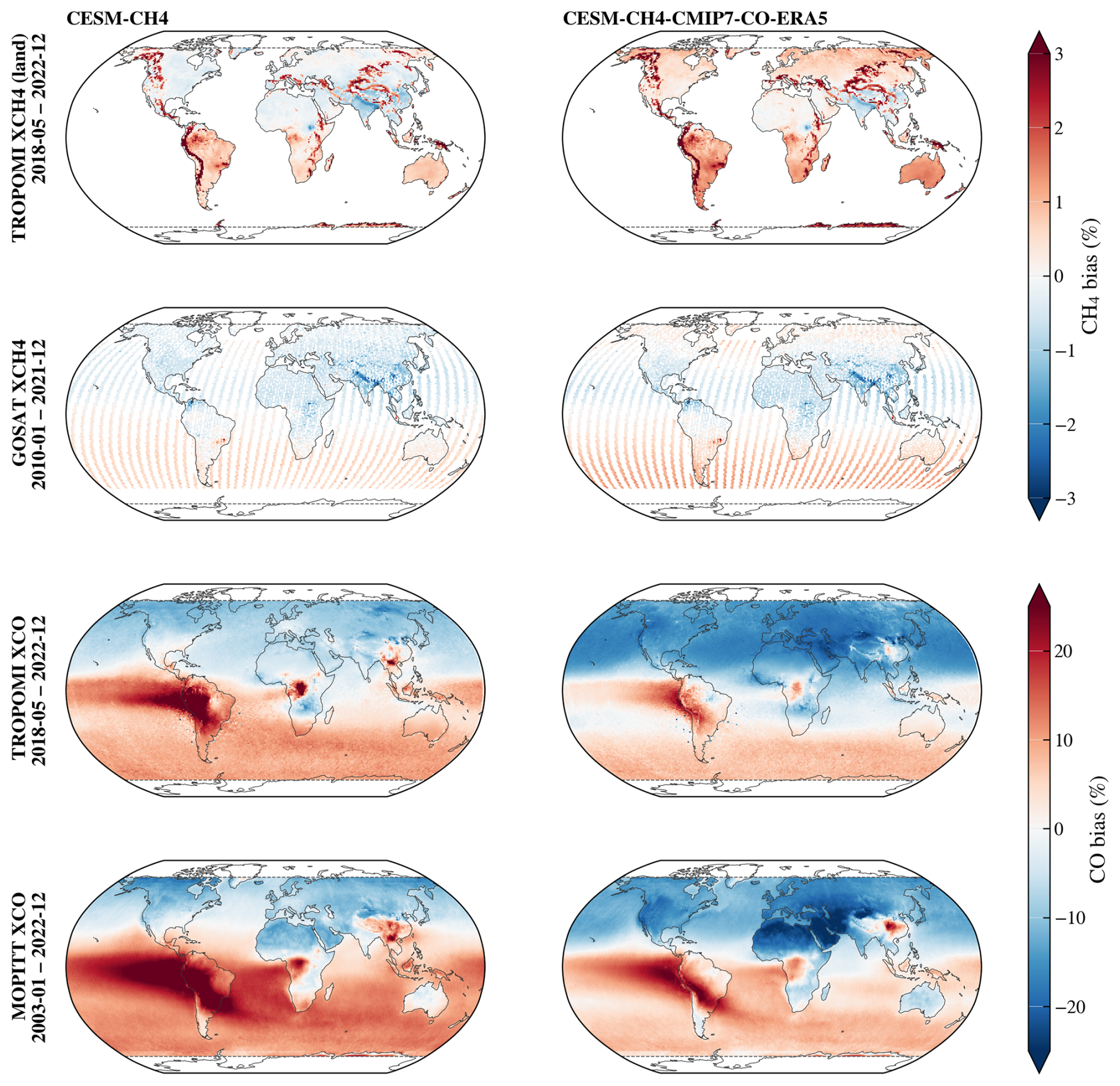
Figure 5 Spatial distribution of the biases for CESM-CH4 (left panel) and CESM-CH4-CMIP7-CO-ERA5 (right panel) against satellite observations for TROPOMI XCH4 (first row), GOSAT XCH4 (second row), TROPOMI XCO ((third row) and MOPITT XCO (fourth row).

The spatial distribution of the biases for CESM-CH4 (left panel) and CESM-CH4-CMIP7-CO-ERA5 is displayed on Fig. 5 for both CO and CH₄ columns. The distribution of the bias is consistent between the two simulations with an underestimation against both GOSAT and TROPOMI, located over India and parts of East Asia, and over Lake Chad (Liu et al., 2026). While GOSAT indicates a low CH₄ bias in the NH, there are patches of CH₄ overestimation in both simulations in comparison to TROPOMI in regions with large topography gradients, e.g., the Andes, the Alps and around the Tibetan Plateau. Both TROPOMI and GOSAT observations indicate that simulations overestimate CH₄ across the SH. There are larger biases in South East Brazil, where emissions are dominated by livestock (Hancock et al., 2025) and across East Africa.

The CO bias has a strong hemispheric asymmetry. The CESM-CH4-CMIP7-CO-ERA5 has a low CO bias in the NH and reaches a 20 % underestimation across North Africa and the Middle East. In contrast, the bias remains within 10 % for the CESM-CH4 simulation. The major CO overestimation occurs in South America for both simulations, with a higher bias in the CESM-CH4 case that is driven by FINN2.5 emissions (Lichtig et al., 2024). The higher CO concentrations over the Congo rainforest and Southeast Asia indicate stronger FINN2.5 emissions while the bias is lower in the GFED4.1s-driven simulation. Overall, TROPOMI and MOPITT indicate the same patterns of CO errors that suggest a good agreement between the two satellite retrievals, but also a consistency of the errors across time periods.

3.3 NOAA Global Greenhouse Gas Reference Network

Figure 6 displays the zonally averaged NOAA marine boundary layer observations over three zonal bands. Based on the aforementioned comparison with four field campaigns, as well as GOSAT, NDACC, and TROPOMI CH₄ observations, we focus here on the three best-performing simulations: CESM-CH4, CESM-CH4-CMIP7-ERA5, and CESM-CH4-CMIP7-CO-ERA5. We added for reference the CT-CH4-2025, which assimilates the observations to estimate emissions using a different OH field and transport model (Oh et al., 2025). The effect of the OH overestimation is clearly illustrated for the CESM-CH4-CMIP7-ERA5 simulation where there is a major offset in CH₄ after 2007, especially for tropical regions. This low bias remains until the end of the simulation period. The CESM-CH4 and CESM-CH4-CMIP7-CO-ERA5 reproduce well the observations, including the long-term trends, interannual variability, and the seasonal cycles overall. It is only for some months where the simulated CH₄ is different from observations, with distinct features in CESM-CH4 and CESM-CH4-CMIP7-CO-ERA5 because of monthly OH differences and potentially transport. These CH₄ disparities are larger and more frequent in the Northern Hemisphere extratropics.

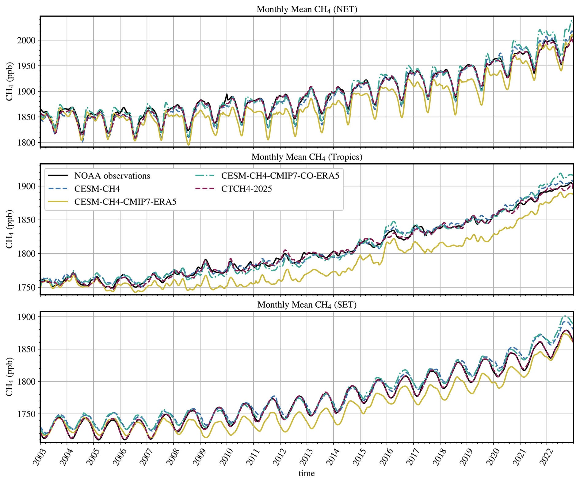
Figure 6 Comparison of simulation and observations of CH₄ with marine boundary layer sites average across zonal latitudinal bands, for Northern Hemisphere extratropics (NET; 30 to 90° N), tropics (−17.5 to 17.5° N), and the SH extratropics (SET; −90 to −30° N).

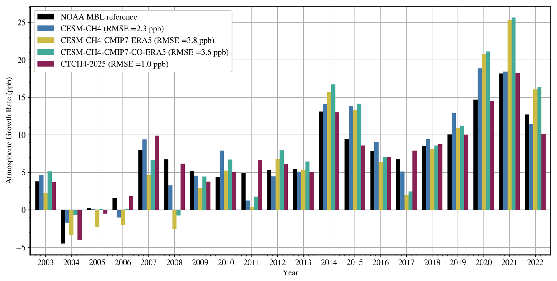
Figure 7 Annual CH₄ growth rate calculated using NOAA GML data extension and integration method.

Figure 7 shows the modelled annual growth rate estimated at NOAA Global Monitoring Laboratory’s MBL sites. The same data extension and integration method is used for MBL reference and modelled trend and growth rate results, allowing a direct comparison of the modelled and observed trends and growth rates. Naturally, as a result of the assimilation of the observations, the CT-CH4-2025 has the best performance. However, we note that differences can be higher than 1 ppb yr⁻¹ for a given year. Compared to CT-CH4-2025, our simulations have a different transport, OH, and soil uptake. The CESM-CH4 and CESM-CH4-CMIP7-CO-ERA5 reproduce well the growth rate, usually within the −3 to +3 ppb yr⁻¹, except for a larger overestimation for the 2020–2021 period. As these simulations are driven by CT-CH4-2025 CH₄ emissions, the overall dynamic of CH₄ growth rate is well simulated, with the pause for the years 2003 to 2006, a renewed growth after 2007, a decreasing growth from 2014 to 2017, followed by a renewed increase that peaks in 2021. Besides emissions, the chemical processes driving the variability of the CH₄ growth rate will be presented in the next sections. We will quantify the role of emissions and chemistry as well as investigate the processes driving the dynamics of the CH₄ growth rate in Sect. 5.

4 Comparison of simulation experiments

4.1 CH₄ budget

Table 2 shows the CH₄ budget for the 2010–2019 period. The chemical lifetime is defined as the ratio of the global, whole-atmosphere CH₄ burden to the tropospheric loss (Saunois et al., 2025), and we also isolate the OH contribution to tropospheric loss. This quantity is conceptually distinct from the perturbation lifetime that describes how a pulse emission decays and is used in global warming potential calculations. The CH₄ chemical lifetime with respect to tropospheric OH varies between 9.4 and 10.5 years, which remains short in comparison to 11.2 ± 1.3 years from Prather et al. (2012). The estimated emissions from the CT-CH4-2025 are on the higher end of the Global Methane Budget ensemble of top-down inversions (Saunois et al., 2025). The soil uptake matches the literature mean estimate that is slightly higher than 30 Tg CH₄ yr⁻¹.

Table 2 CH₄ budget (2010–2019). The tropospheric chemical loss (L_chem) is calculated for all the reactions in the troposphere and for the CH₄+OH reaction in parenthesis. The chemical lifetime is the total atmospheric burden divided by the tropospheric sink, also with CH₄+OH reaction only in parentheses. L_dep is the loss of CH₄ by soil uptake. All the units are Tg CH₄ yr⁻¹, except for CH₄ lifetime in years.

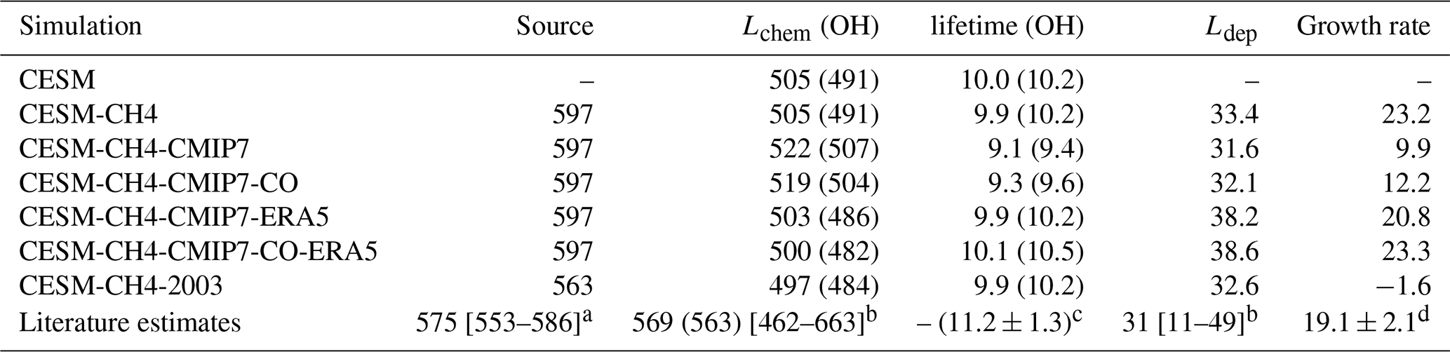
^a Top-down range of the Global CH₄ Budget (Saunois et al., 2025). ^b Bottom-up estimates for tropospheric OH and Cl loss (range given for OH only) compiled by the Global CH₄ Budget (Saunois et al., 2025). ^c 2010 tropospheric CH₄ lifetime with regard to OH estimated by Prather et al. (2012). ^d Growth rate estimated from CH₄ observations from the Global Monitoring Laboratory (Lan et al., 2024) and converted to Tg CH₄ yr⁻¹ using a conversion factor of 2.77 Tg CH₄ ppb⁻¹ (Lan et al., 2021b; Nisbet et al., 2023).

The CESM-CH4, CESM-CH4-CMIP7-ERA5 and CESM-CH4-CMIP7-CO-ERA5 chemical lifetime are well within the uncertainty range of the empirical estimate. As a result, the combination of slightly higher emissions and higher OH leads to an average growth rate that is close to the one derived by NOAA observations over the 2010–2019 period for the CESM-CH4, CESM-CH4-CMIP7-ERA5 and CESM-CH4-CMIP7-CO-ERA5. The range of tropospheric CH₄ loss to OH is between 482 and 491 Tg CH₄ yr⁻¹, which is much lower than the values estimated by the suite of chemistry-climate models reported in Saunois et al. (2025). The emission-driven simulations with an OH overestimation thus underestimate the CH₄ atmospheric growth rate.

4.2 CO budget

The CO budget is displayed in Table 3. Total direct emissions from Gaubert et al. (2024), FINN2.5, direct MEGAN CO, and a minor oceanic source sum to 1373 Tg CO yr⁻¹. This is much higher than 848 Tg CO yr⁻¹ quantified by Tang et al. (2026), but only slightly higher than 1200 Tg CO yr⁻¹ estimated by Zheng et al. (2019). Similarly, our total sources (Source +P_total) are 2906 Tg CO yr⁻¹ in CESM-CH4 and 2657 Tg CO yr⁻¹ in CESM-CH4-CMIP7-CO-ERA5, higher than 2395 Tg CO yr⁻¹ from Tang et al. (2026) and 2600 Tg CO yr⁻¹ from Zheng et al. (2019). Despite different OH, biogenic emissions and CH₄, the CO chemical production does not change by a large amount when switching emission inventories. However, using different meteorological fields led to an additional CO chemical production (P_total) of 100 Tg CO yr⁻¹, which when combined with a different loss increased by 75 Tg CO yr⁻¹, led to a longer lifetime of 5 d, slightly less than a 10 % increase. The higher CO emissions in CESM-CH4 occur almost everywhere except over China and at high latitudes in Canada and Siberia (Fig. 8). This is likely to be driven by a stronger and more realistic decline in CO emissions in China in the CEDS-CMIP7 than in our posterior CO emissions, where the trend is based on the CAMS-GLOB-ANTv5.3 dataset, which does not show a strong decline in Chinese emissions. However, the CEDS-CMIP7 emissions might still be underestimated in northern China (Fig. 5), although it is difficult to interpret because of the fire emissions that could be biased differently. As already discussed, the FINN2.5 emissions are the main drivers of higher CO emissions across the tropics. The maps suggest this is accompanied by a stronger chemical production in Southeast Asia, Southern Mexico, the Amazon, the island of Borneo and parts of the Congo Rainforest. Many of these places are likely to also be driven by VOCs emitted by FINN emissions. Conversely, there are large areas where CESM-CH4 has a lower chemical source than the CESM-CH4-CMIP7-CO-ERA5 simulation, which results from lower biogenic emissions in the tropics (Fig. S1 in the Supplement). The net effect is a higher CO loss in CESM-CH4 for the period 2003–2022 that is mainly driven by the fire emissions. This suggests rapid changes between fire, biogenic and anthropogenic emissions that interplay closely on the CO budget, highlighting the need to reduce uncertainties for all of these sources. As anthropogenic and fire CO emissions decline, the attribution of the primary and secondary source of CO will become even more difficult to address. The drivers of chemistry changes will be presented in the next section.

Table 3 CO budget (2010–2019). P_total is the total chemical production. $P_{{\mathrm{CH}}_{\mathrm{4}}}$ is the CO chemical production from CH₄ oxidation assuming a yield of 75 % (Gaubert et al., 2016). All units are Tg CO yr⁻¹, except chemical lifetime (days) and burden (Tg CO).

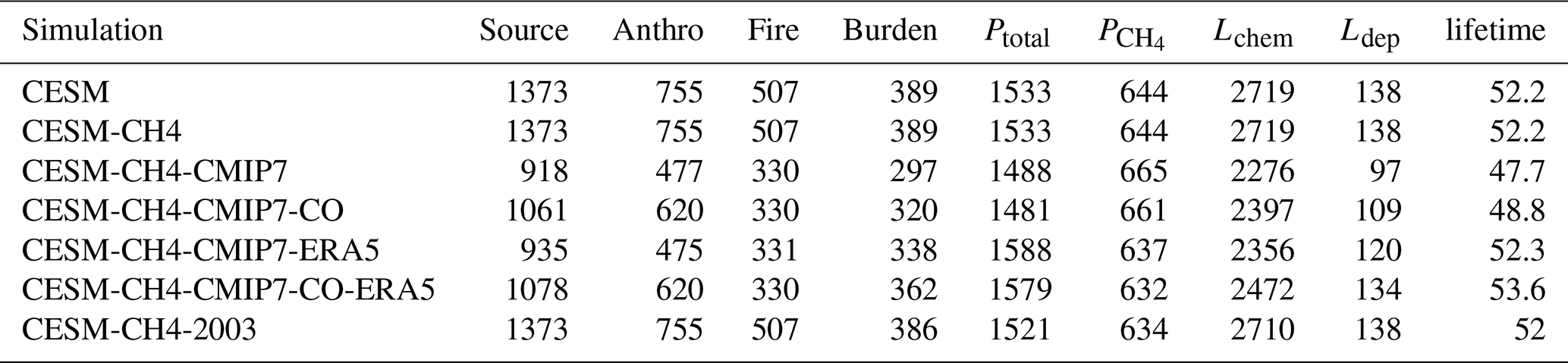
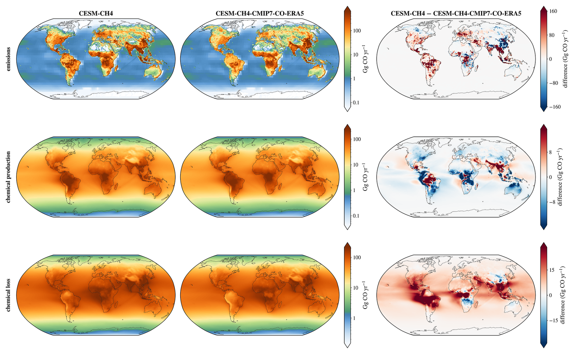
Figure 8 Spatial distribution of the 2003–2022 mean CO flux estimates (Gg CO yr⁻¹ per grid cell) for (top) total emissions, (middle) chemical production and (bottom) chemical loss, for (left) CESM-CH4, (center) CESM-CH4-CMIP7-CO-ERA5 and (right) their difference (CESM-CH4 − CESM-CH4-CMIP7-CO-ERA5).

4.3 Drivers of chemistry changes

We investigate the impact of the model configurations and external forcings (i.e., CH₄ emissions, chemistry emissions, choice of meteorological reanalysis) on the OH budget and other related chemical fluxes. Figure 9 displays the changes in the OH sources and loss for various pairs of experiments. First, we contrast the changes if CH₄ emissions had remained at 2003 levels (Fig. 9A). This CH₄ emission scenario leads to a reduction in CH₄ burden by 1.5 %, reducing the OH loss, increasing OH burden, thus effectively shortening the CH₄ lifetime, and reduces O₃ formation, in line with previous studies (Prather et al., 2001; Fiore et al., 2002; Shindell et al., 2005). It directly reduces CO formation from CH₄ by 1.5 % and the OH changes shorten the CO lifetime. This reduced CO lifetime is illustrated by a lower primary CO despite the CO emissions being the same. Contrary to Staniaszek et al. (2022), HO₂, O₃ and HO₂+O₃ reaction all decrease following a CH₄ decrease. We also found a small reduction in other channels of OH production that are not related to O₃, NO + HO₂, VOCs and the H₂O₂ photolysis, some of which might be related to the reduction in products of the CH₄ oxidation.

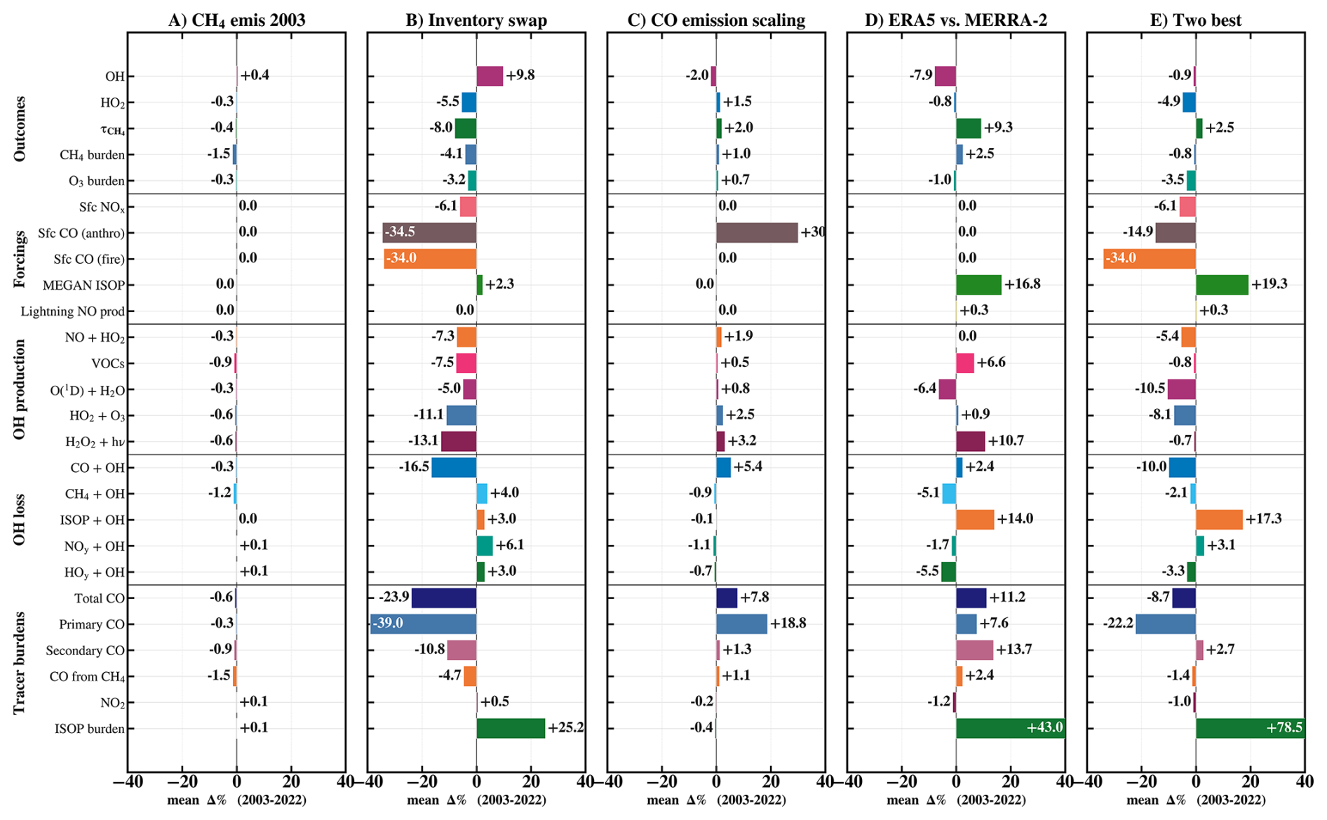
Figure 9 Differences in abundance for the various pairs of experiments: (A) CESM-CH4-2003 – CESM-CH4, (B) CESM-CH4-CMIP7 – CESM-CH4, (C) CESM-CH4-CMIP7-CO – CESM-CH4-CMIP7, (D) CESM-CH4-CMIP7-CO-ERA5 – CESM-CH4-CMIP7-CO, (E) CESM-CH4-CMIP7-CO-ERA5 – CESM-CH4.

Second, we look at the impact of changing anthropogenic and fire emission inventories of non CH₄ species (Fig. 9B), as shown in Fig. 2. In the CESM-CH4-CMIP7, emissions of NO_x, CO and of most NMVOCs are lower. The reduction in fire and anthropogenic sources of CO, combined with a lower secondary CO, leads to a net 16.5 % reduction in OH loss due to CO, which seems to be a dominant driver of the OH increase. However, the net change in NMVOCs, CO and NO_x appears to reduce O₃ and HO₂, thus lowering the OH source. Despite having the same nudging in both cases, the isoprene emissions are 2.3 % higher, likely due to reduced aerosol emissions from fires (Fig. 2) interacting with radiation. Figure S2 shows that the CESM-CH4-CMIP7 −- CESM-CH4 isoprene difference is small compared with the meteorology-driven change (Fig. S1). The lower NO_x emissions directly reduce the OH chemical production through NO_x recycling source. The net impact of emission change is an OH increase.

Third, we examine a 30 % perturbation of CO emission (Fig. 9C). The results are in line with Gaubert et al. (2016), where the primary impact of CO increase is an OH reduction, which decreases the other OH losses and thus effectively increases CH₄ lifetime. Also, the secondary feedback is an increase in O₃, in the presence of NO_x and H₂O₂, more efficiently recycling OH and reducing the impact of the perturbation.

Fourth, we analysed the impact of meteorology, by contrasting nudging to ERA5 and MERRA-2 reanalyses (Fig. 9D). We found that the simulation with ERA5 has 7.9 % less OH than the one driven by MERRA-2, resulting in a 9.3 % longer CH₄ lifetime and 2.5 % increase in burden. This result is consistent with differences in global annual mean OH levels driven by meteorological forcings (Gaubert et al., 2017; He et al., 2021). The main driver is the large increase of MEGAN isoprene emissions by +16.8 % (Fig. 2), driven by higher temperatures in the ERA5 nudged simulation (Fig. S1). This leads to a higher isoprene burden (+43 %) and isoprene+OH loss (+14 %). The latter led to a larger secondary CO burden (+13.7 %) and subsequent CO+OH loss (+2.4 %). While there is a net increase in the VOC and H₂O₂ sources of OH, there is also a net decrease in O₃ and thus primary OH formation (−6.4 %). The meteorology also led to a net reduction in OH loss through radical–radical reactions (−5.5 %). Clearly, the impact of emissions from vegetation simulated by MEGAN is the main process behind the large changes in the oxidative power of the atmosphere with around 9 % change in CH₄ lifetime. Finally, the comparison between the two best experiments: CESM-CH4-CMIP7-CO-ERA5 and CESM-CH4, reflects the combined effect of the chemical emissions although with the impact of CO scaling, and meteorology previously described, with notable cancellation of CO and isoprene emissions.

4.4 OH budget

Lelieveld et al. (2002) assessed the role of the O₃ photolysis source of OH as primary production (P) as opposed to radical driven OH formation (secondary, S) and introduced the concept of OH recycling probability r, defined as $\mathrm{1}-P/G$, with $P/G$ the ratio of the primary to the total gross production G, in Tmol yr⁻¹. For higher OH recycling probability, with r values larger than 0.5, the tropospheric chemistry system is not as dependent on changes in ozone and other parameters related to primary production. It is also more resilient to CH₄ and CO perturbations. Figure 10 displays the tropospheric OH budget for 2013, with the total production and loss (Tmol yr⁻¹) and the relative contribution (%) of each reaction family.

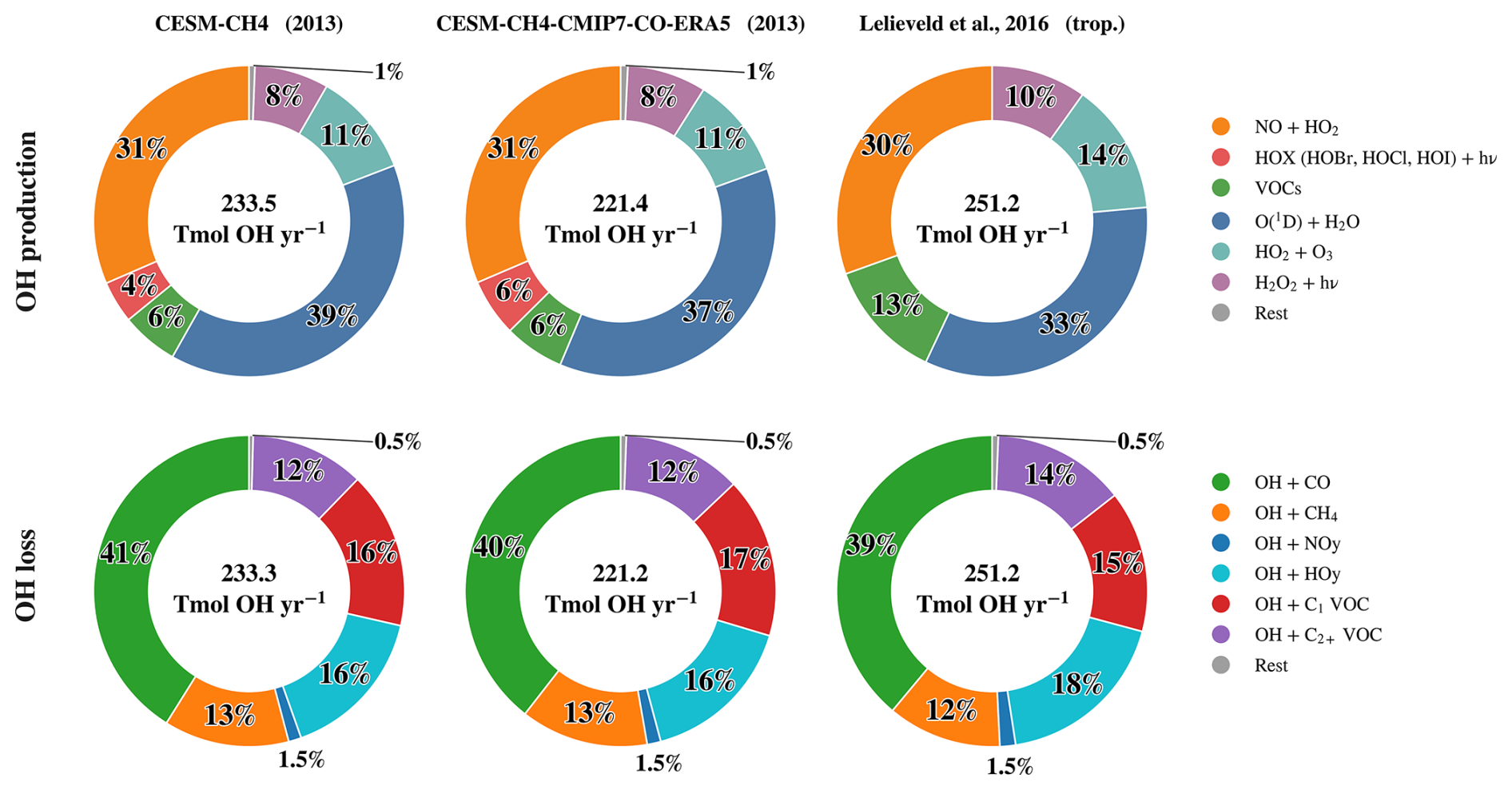
Figure 10 OH budget for the year 2013 by source (first row) and loss (second row) in Tmol yr⁻¹ with the contribution of each family defined in Lelieveld et al. (2016). Primary OH production is O(¹D)+H₂O. Secondary production comes from NO+HO₂, HO₂+O₃, H₂O₂ photolysis, VOCs (photolysis of OVOCs plus ROOH+OH and RO₂+HO₂), and photolysis of the hypohalous acids HOBr, HOCl and HOI (HOX). OH loss is grouped by reactant: CO, CH₄, single-carbon compounds other than methane and CO (C₁: CH₂O, CH₃OH, CH₃OOH, HCOOH and CH₃O₂), organics with two or more carbon atoms (C₂₊), HO_y and NO_y. Minor channels (alkene ozonolysis, NO_y photolysis, and reactions with halogens, sulfur species and nitriles) are grouped as “rest”.

We compare the OH budget for the year 2013 with the results from Lelieveld et al. (2016). Bossolasco et al. (2025) provided a comprehensive evaluation of the impact of the inclusion of SLH representation in CESM1 and estimated a value for r of nearly 60 %, indicative of a naturally resilient atmospheric oxidising capacity. Our estimates of r (0.63 and 0.61 for CESM-CH4-CMIP7-CO-ERA5 and CESM-CH4, respectively) are consistent with Bossolasco et al. (2025). We found that the relative (%) contribution of each OH production pathway remains fairly consistent with Bossolasco et al. (2025), i.e., between CESM1 and CESM2. Our relative and absolute contribution of the additional source of OH through halogen photolysis is also consistent. However, their estimate for the OH budget for climatological year 2000 is 173.7 Tmol yr⁻¹, which is much smaller than our estimates between 221 and 234 Tmol yr⁻¹ for the year 2013. This could be driven by the addition of VOCs and OVOCs in the MOZART‐T1 mechanism (Emmons et al., 2020), which contribute to both the sources and losses of OH. Differences in emissions, simulated year and model structure between CESM1 and CESM2 likely also contribute.

Lelieveld et al. (2016) used the Mainz Organic Mechanism (MOM) and included a significantly larger number of species, of the order of several hundred. While their range of isoprene emissions (546–578 Tg C yr⁻¹) is only slightly higher than our model simulations (on average 545 Tg C yr⁻¹ when driven by ERA5), they found a much higher source of OH from VOCs, more than twice ours, 31.4 Tmol yr⁻¹ (13 %) against 13.8 Tmol yr⁻¹ (6 %). This is likely driven by the more explicit representation of OH recycling pathways in MOM, whereas MOZART-T1 represents the products of the OH+ isoprene reaction with only a few lumped species. They also have a relatively higher contribution from H₂O₂ photolysis and HO₂+O₃, but a lower O₃ photolysis. It also highlights the dual role of VOC oxidation as both a source and a sink of OH. Incomplete VOC oxidation chemistry in our simulations would also underestimate secondary CO production. This could explain part of the model’s CO and CH₄ underestimation without requiring higher anthropogenic or fire CO emissions. Otherwise, their relative family contributions are similar to our simulations. This reinforces the need to integrate complex chemistry mechanisms to fully understand the OH budget, integral to the quantification of the variation in CH₄ oxidation. In particular, it underlines the role of short-lived halogens and volatile organic compounds such as isoprene on the OH budget.

4.5 Spatial distribution of OH

Next, we compare with the OH spatial distribution from Spivakovsky et al. (2000). This OH estimate is a reference and has been commonly prescribed in CH₄ inversions, after scaling the field by 0.9 in the NOAA CarbonTracker-CH4-2025 inversion and 0.92 in the TRANSCOM-CH4 experiment (Patra et al., 2011), values that fit better the methyl-chloroform inversions after 2000 (Huijnen et al., 2010; Montzka et al., 2011). The globally averaged annual means (2003–2022) simulated OH of 9.93×10⁵ molec. cm⁻³ (CESM-CH4) and 9.79×10⁵ molec. cm⁻³ (CESM-CH4-CMIP7-CO-ERA5) are on average remarkably close to the Spivakovsky estimate of 9.80×10⁵ molec. cm⁻³ (Fig. 11). The simulated OH is higher in the NH than in the SH, a feature documented in many atmospheric chemistry models (Naik et al., 2013; Zhao et al., 2019; Stevenson et al., 2020), while the Spivakovsky OH with a ratio of 1 between the two hemispheres tends to be better. Their OH is much higher across the tropical rain forests of the Amazon, the Congo and in New Guinea and Indonesia. This is due to their older isoprene mechanism and much lower isoprene emission that amount to 350 Tg C yr⁻¹ compared to roughly 500 Tg C yr⁻¹ when averaging our two simulations. Their isoprene and NMHC contributions (with a simulation that omits them) to the net loss of OH were only 3 % and 7 %, respectively. As mentioned above, it is around 29 % in our case. As a result of the active photochemistry and high emissions from anthropogenic, and eventually biogenic and fire sources, the simulated OH is much higher in the lower latitude of the NH, across Mexico, the Arabian Peninsula, India and Southeast Asia. Since the global average OH is no longer biased, future work should investigate how our modeled OH impacts the distribution of regional emission estimate by CH₄ observations. We further compare the simulated vertical profiles with the ATom OH (Fig. S3) estimates (Brune et al., 2020). The simulations represent OH well within the uncertainty range of the observations, except that OH is overestimated in spring during ATom-4 at higher altitude in the northern extratropics.

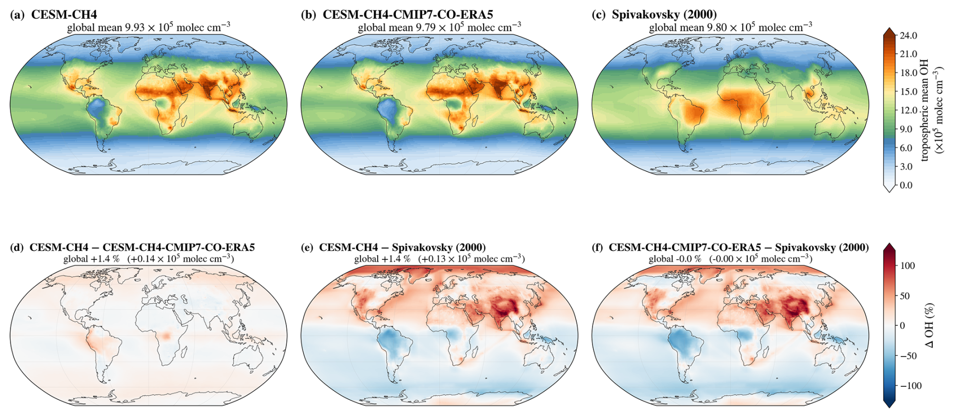
Figure 11 Spatial distribution of the 2003–2022 mean airmass-weighted tropospheric OH concentration (10⁵ molec. cm⁻³) for (left) CESM-CH4, (center) CESM-CH4-CMIP7-CO-ERA5 and (right) the Spivakovsky et al. (2000) climatology scaled by 0.901. The bottom panels show the relative differences (%).

The spatial distribution of the chemistry terms is a result of large differences in the OH budget, integrating many different factors combined (Fig. 9). Despite a few percent differences between the two simulations (Fig. 11), that averages globally to a 1.4 %, the CESM-CH4 has both higher global OH source and loss than CESM-CH4-CMIP7-CO-ERA5 by around 5.8 % (Fig. 12). The spatial distribution of the OH budget terms varies by channels and shows spatial heterogeneity. The primary OH production as well as recycling from the NO+HO₂ and HO₂+O₃ are all higher in CESM-CH4, and show maximum around the Amazon and the Congo basins, across the equator and over the Antarctic continent. They also tend to be higher over the oceans and at high latitudes. Conversely the OH production is lower across parts of the mid-latitude, mainly over the continents. The VOCs, H₂O₂, and more prominently the hypohalous acids source of OH show more widespread reduction in OH production (−22 %). This is driven by higher Cl when the ERA5 reanalysis is used for nudging (Fig. S7), effectively reducing the halogens photolysis source of OH in CESM-CH4-CMIP7-CO-ERA5. The higher OH in the northern high latitude and parts of the tropics is causing a higher CH₄ loss in these regions while a lower OH reduces CH₄ loss in central Asia and over the remote oceans. Higher CO and VOCs emissions in CESM-CH4 trigger a widespread increase in the CO+OH loss in most parts of the world, which is more pronounced in these high latitudes and from fires over the Amazon, Congo and across Southeast Asia. These features from the fires trigger higher values across the OH loss terms as well as OH recycling source, and appear to be the drivers for higher OH sources and sinks in the CESM-CH4 simulation.

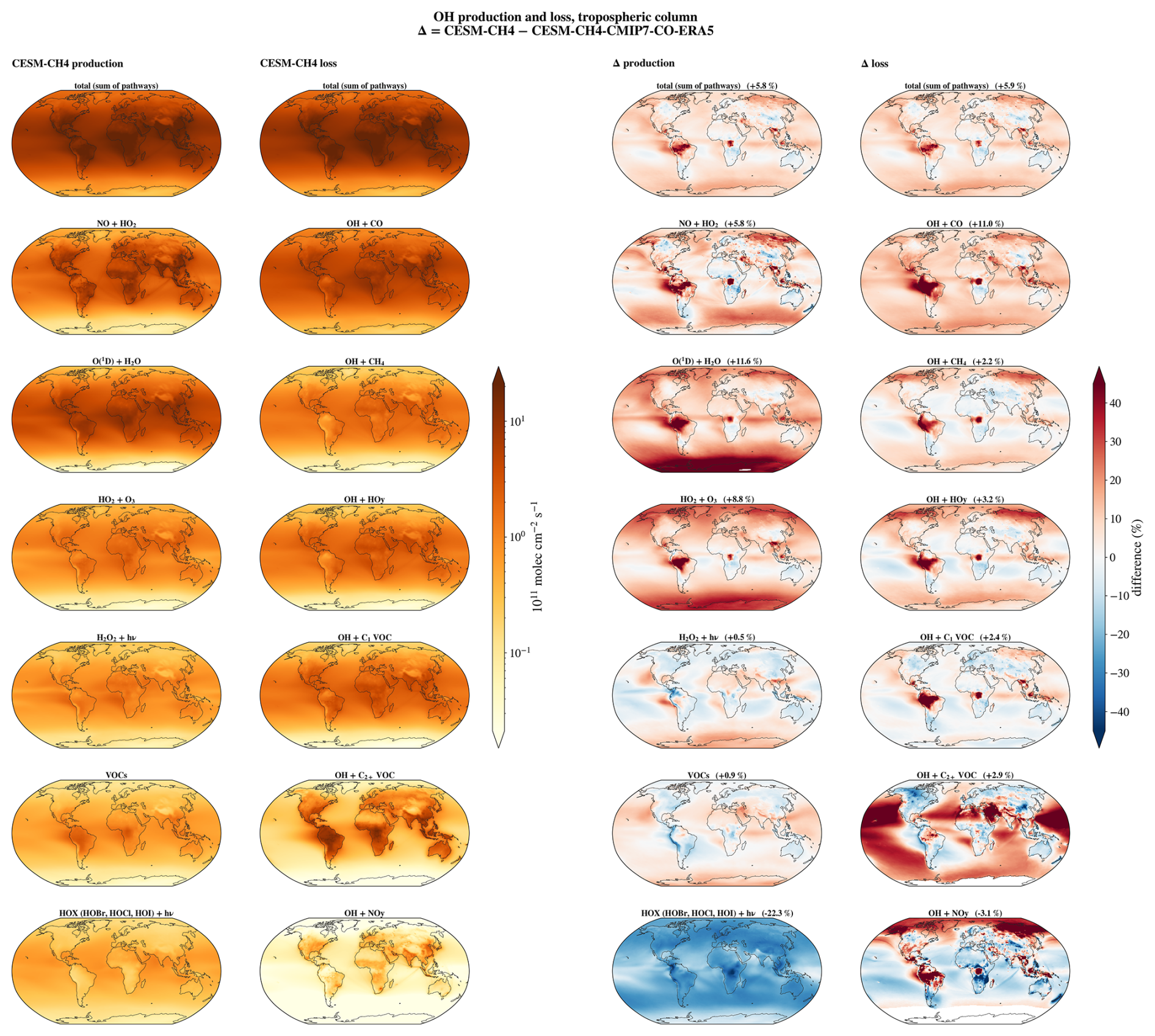
Figure 12 Spatial distribution of the OH sources and loss for CESM-CH4 (leftmost columns) and the relative differences between CESM-CH4 and CESM-CH4-CMIP7-CO-ERA5 for each of the OH terms (rightmost columns).

5 Decomposition of the drivers of the CH₄ Atmospheric Growth Rate

Figure 13 links the simulated CH₄ growth-rate variability to the simulated evolution of tropospheric OH in the two best-performing configurations. Panel (a) shows annual OH anomalies (relative to the 2003–2022 mean) together with the ENSO phase, while panels (b), (c) decompose the year-to-year change in the CH₄ growth rate (ΔGR) into its individual budget terms and compare the simulated changes with the NOAA record. The blue bars isolate the oxidation contribution, −m Δk, allowing the role of OH variability to be distinguished from that of emissions. Following Qu et al. (2022), the decomposition of the CH₄ growth rate changes is defined as:

$$\begin{array}{}\text{(R3)}& {\displaystyle \frac{{\mathrm{d}}^{\mathrm{2}}m}{\mathrm{d}{t}^{\mathrm{2}}}}={\displaystyle \frac{\mathrm{d}E}{\mathrm{d}t}}-m{\displaystyle \frac{\mathrm{d}k}{\mathrm{d}t}}-k{\displaystyle \frac{\mathrm{d}m}{\mathrm{d}t}}-{\displaystyle \frac{\mathrm{d}L}{\mathrm{d}t}}\end{array}$$

where m is the atmospheric CH₄ burden, E the emissions, k the OH loss frequency, and L the non-OH sinks. Accordingly, each change in CH₄ growth rate is the annual sum of an emission term (ΔE), an OH-driven oxidation term (−m Δk), a first-order relaxation term (−k Δm), and changes in non-OH sinks (−ΔL). The value plotted for year t represents the change from the previous year (t−1) to the current year (t). For Δk and Δm, the value is evaluated as the differences between December–January mean burden, and m is the mass at the beginning of the studied year, calculated from the December–January mean as well. These four contributions are listed beneath each panel in Fig. 13 and reproduce ΔGR. This attribution follows Qu et al. (2022), which Chen et al. (2025) identified as the preferred approach because it partitions the two physical forcing terms (ΔE and −m Δk) while preserving budget closure. Because both experiments use the same CT-CH₄-2025 surface CH₄ emissions, the ΔE term is identical. Since the −k Δm and −ΔL terms are comparatively small, the differences between the two simulations arise almost entirely from their different representations of OH variability.

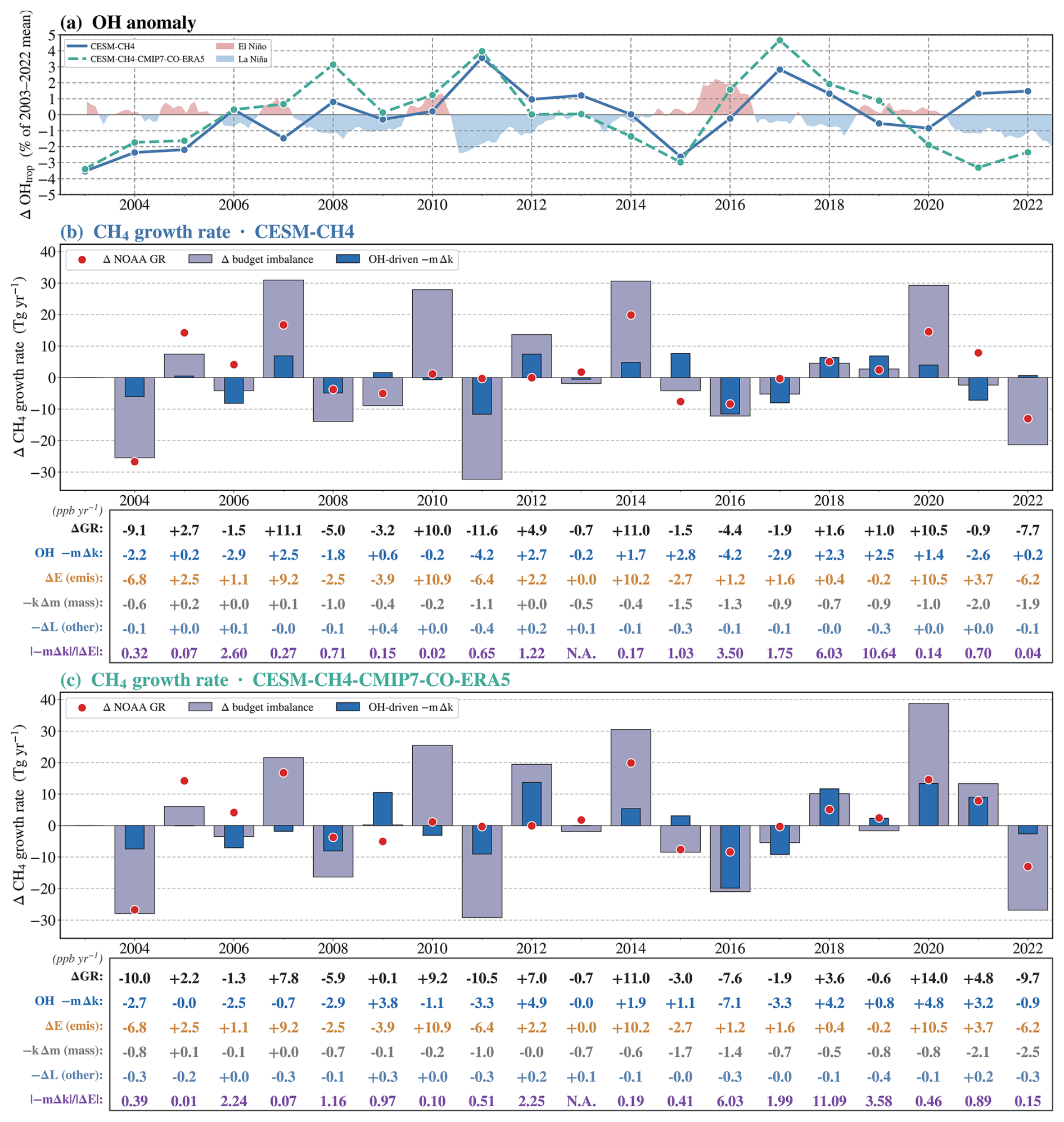
Figure 13 Inter-annual OH anomaly and its contribution to the CH₄ growth rate. (a) OH anomaly (% of the 2003–2022 record mean) for CESM-CH4 and CESM-CH4-CMIP7-CO-ERA5, with ENSO phases shaded. (b, c) Year-to-year change in the CH₄ growth rate: ΔGR (grey bars), the change in the NOAA rate (red points) and the OH-driven term −m Δk (blue bars). The table lists $\mathrm{\Delta }\mathrm{GR}=\mathrm{\Delta }E-m\mathrm{\Delta }k-k\mathrm{\Delta }m-\mathrm{\Delta }L$ (ppb yr⁻¹) and the ratio $|-m\mathrm{\Delta }k|/\left|\mathrm{\Delta }E\right|$.

The interannual variability in tropospheric OH exhibits a negative correlation with ENSO (e.g., Turner et al., 2018; Patra et al., 2021; Anderson et al., 2021), with enhanced OH during La Niña (Murray et al., 2013) and reduced OH during El Niño (Prinn et al., 2001, 2005; Duncan et al., 2003). The slope of the OH time series determines the sign of the oxidation contribution to methane growth. An increasing OH strengthens the CH₄ oxidation and lowers the growth rate ($-m\mathrm{\Delta }k<\mathrm{0}$), whereas decreasing OH weakens oxidation and increases CH₄ growth. The most prominent examples of oxidation-dominated variability coincide with major ENSO transitions. For instance, during the 2010–2012 La Niña, OH increased rapidly to its highest value of the record, producing strong negative oxidation anomalies in 2011 (−4.2 and −3.3 ppb yr⁻¹). OH reaches a minimum in 2015 before increasing rapidly into the 2017 maximum, making 2016 the year with the largest OH-driven change, with oxidation contributions of −4.2 and −7.1 ppb yr⁻¹ and forcing ratios of 3.5 and 6.0 in the two simulations.

The relaxation term −k Δm is consistently negative in response to positive emission growth. It is often relatively small, but can reach values between −1 and −2 (2011, 2015, 2021) following years with strong emission changes as estimated by the CT-CH4-2025 (2010, 2014, 2020). By contrast, changes in soil uptake remain negligible throughout the record ($\left|\mathrm{\Delta }L\right|<\mathrm{0.5}$ ppb yr⁻¹), confirming that interannual variability of the CH₄ sink is controlled almost entirely by OH chemistry in our model. The bottom row gives the ratio $|-m\mathrm{\Delta }k|/\left|\mathrm{\Delta }E\right|$, which measures the relative importance of oxidation and CH₄ emission forcing and it is undefined in years when ΔE≈0. Overall, emissions determine most of the large interannual growth-rate anomalies while OH variability acts primarily as a modulator that either amplifies or offsets the emission-driven tendency. Over the 18 growth rate accelerations calculated here (the ratio is undefined for 2013), the OH oxidation is the dominant term 7 times, with both simulations agreeing for 6 common years (2006, 2012, 2016, 2017, 2018 and 2019). Conversely, the sharp decline in CH₄ growth in 2004 agrees closely with the observed decrease and is primarily driven by reduced emissions, while increasing OH provides an additional negative contribution. The large positive growth-rate anomalies in 2010 and 2014 arise almost entirely from enhanced emissions, with oxidation playing only a minor role. Regarding 2020, the OH-driven forcing is +1.4 ppb yr⁻¹ (≈4 Tg yr⁻¹) in CESM-CH4 and +4.8 ppb yr⁻¹ (≈13 Tg yr⁻¹) in CESM-CH4-CMIP7-CO-ERA5, corresponding to about 12 % and 31 % of the combined emission-plus-OH forcing (ΔE−m Δk). The CESM-CH4 value is close to the 5 Tg yr⁻¹ (14 %) from Qu et al. (2022), whereas the ERA5 configuration roughly doubles this contribution, up to 46 %, in line with other studies (Stevenson et al., 2022; Peng et al., 2022; Chen et al., 2025).

The most informative period is the 2020–2022 triple La Niña because it departs from the canonical ENSO–OH relationship. In CESM-CH4, OH increases as expected during La Niña, producing a negative oxidation contribution that largely offsets the emission increase and keeps the simulated CH₄ growth rate close to the NOAA observations (Figs. 6 and 7). In contrast, CESM-CH4-CMIP7-CO-ERA5 simulates a continued decline in OH despite persistent La Niña conditions. Integrated over 2020–2022, the cumulative OH contribution is close to zero in CESM-CH4 but approximately +7 ppb yr⁻¹ in CESM-CH4-CMIP7-CO-ERA5, indicating that uncertainty in meteorologically driven OH variability alone can account for roughly one-fifth of the simulated CH₄-growth anomaly. Figure S8 splits the difference between the two experiments into an emission change under the same meteorology (CESM-CH4-CMIP7-CO − CESM-CH4) and a switch of the reanalysis nudging field (CESM-CH4-CMIP7-CO-ERA5 − CESM-CH4-CMIP7-CO). It shows that meteorology dominates in 2020–2022 and in the early 2000s, whereas anthropogenic and fire emissions matter more in 2016–2019. Consistent with this, Fig. 2 shows that lightning emissions under ERA5 are often higher, but lower during 2020–2022. The nudging to ERA5 leads to lower lightning in East Africa and across South America (except for the Amazon basin) and across the SH while ERA5 leads to higher lightning in India, Indonesia and parts of West Africa and the Amazon basin (Fig. S4).

Overall, this highlights the importance of correctly representing chemistry-meteorology interactions and reducing their uncertainties, which will be the focus of future research. However, we will further investigate the drivers of OH changes in the next section.

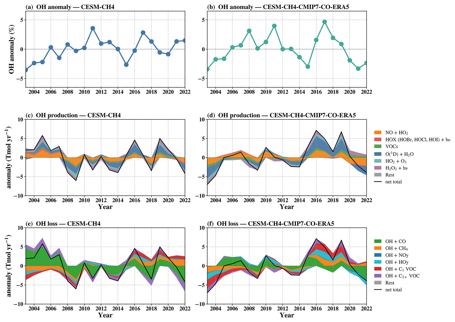
Figure 14 Tropospheric OH budget over 2003–2022 by reaction channel, for CESM-CH4 (left) and CESM-CH4-CMIP7-CO-ERA5 (right). (a, b) OH anomaly (%), (c, d) production and (e, f) loss channels (Tmol yr⁻¹), all relative to the 2003–2022 mean stacked about zero with the net as the black line.

6 Attributing the OH budget changes to their drivers over time

The growth-rate decomposition of Sect. 5 and Fig. 13 attributes a variable part of the CH₄ growth rate to the inter-annual OH anomaly. Here we explain that anomaly. Figure 14 shows the temporal change of OH budget terms with the annual anomaly of every reaction channel. The result reflects the most important drivers of the OH budget outlined in the previous sections, with NO+HO₂ and O(¹D)+H₂O being the main source and CO the main loss. Interestingly, the importance of the buffering effect is highlighted by the fact that higher variability in chemical fluxes does not always lead to higher OH anomalies, and the highest OH anomalies do not necessarily correspond to strong chemical flux anomalies.

To further understand these temporal changes, we perform a regression of the OH anomalies on its drivers. The regression is carried out by region and aggregated globally by weighting each region by CH₄+OH loss following Lawrence et al. (2001), so that the attribution reflects the oxidizing capacity that controls CH₄ removal. The weighting, and its robustness to alternative choices (air mass and OH burden), is detailed in Sects. S1–S2 and Fig. S9 in the Supplement. The first regression is against forcings (surface NO_x, anthropogenic and fire CO, isoprene and sector-tagged CH₄ emissions) as well as meteorology related terms: lightning NO, the O₃→O(¹D) photolysis frequency J(O₃) and water vapour (Fig. 15). The second regression is based on reactant abundances such as CO, NO₂, O₃, isoprene and CH₄ (Fig. 16). The two bases reconstruct ≈69 % and ≈91 % of the global OH variance for CESM-CH4-CMIP7-CO-ERA5, and ≈66 % and ≈87 % for CESM-CH4 (Fig. S10). These regressions are used to explore the drivers of OH anomalies alongside the production and loss pathways diagnosed from the model budget. All predictors within each basis are fitted jointly in each region, so adding their fitted terms to reconstruct the OH anomaly does not require independence. However, correlated predictors cannot be fully separated and their terms are conditional associations rather than independent contributions (Figs. S13 and S14). We quantify this with the variance inflation factor, ${\mathrm{VIF}}_j=\mathrm{1}/(\mathrm{1}-R_j^{\mathrm{2}})$, where $R_j^{\mathrm{2}}$ is obtained by regressing predictor j on the other predictors of the same band (VIF =1 if uncorrelated; Figs. S13 and S15). The leading contributions (lightning NO, isoprene and, in CESM-CH4-CMIP7-CO-ERA5, surface NO_x) come mainly from the tropical bands (Fig. S16). Where predictors share anthropogenic or fire sources, such as surface NO_x and CO, their strong correlation in some bands increases the uncertainty of their individual contributions, which are therefore better interpreted as a combined emission contribution (Figs. S14 and S15). We found little explanatory power of CH₄ emissions on the OH temporal variability throughout the period and they cannot be fully separated from the CO terms. The OH signal is set mainly by NO_x, CO and ozone photochemistry rather than by the CH₄ fluxes (Fig. 15). Contrary to CH₄ emissions, the steadily increasing CH₄ burden appears to drive a consistent reduction in OH (Fig. 16), accompanied by an increase in CH₄+OH (Fig. 14), rather than year-to-year fluctuations.

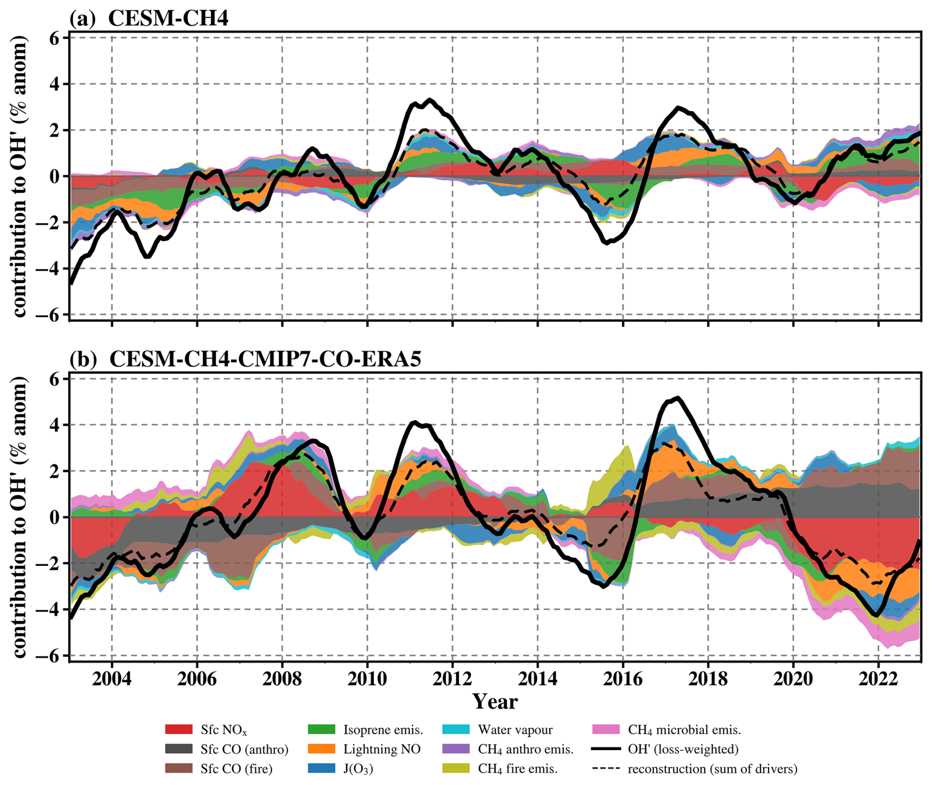
Figure 15 Driver contributions to the global, loss-weighted OH anomaly in the forcing basis, for (a) CESM-CH4 and (b) CESM-CH4-CMIP7-CO-ERA5. Bands are the stacked per-driver contributions (% anomaly). The black line is OH^′ and the dashed line its reconstruction (the sum of the coloured bands).

The study period opens with both configurations at their most negative OH anomaly (about −3.5 % in 2003), but for opposite budget reasons. In CESM-CH4 the high early-record CO burden keeps the CO+OH sink large (Fig. 14e) and holds OH down, and the regression assigns this suppression to the CO burden (Fig. 16a) and, in the forcing basis, to fire CO (Fig. 15a), as FINN emissions are high and are declining during this period. In CESM-CH4-CMIP7-CO-ERA5, the negative OH anomalies are driven by weak primary production, with O(¹D)+H₂O and the NO_x-recycling source both negative (Fig. 14d). In this case, the concomitant strong decline in anthropogenic CO and increase in anthropogenic NO_x emissions (Fig. 15b) explain the consistently positive OH trends between 2003 and 2009. The two runs therefore track one another in these years, though driven by different chemical terms and forcings. The differences in surface NO_x emissions might explain the larger role of NO_x in the simulation driven by CMIP7 emissions (CESM-CH4-CMIP7-CO-ERA5, Fig. 2). Until 2009, the CESM-CH4 indicates an increase in OH that is driven by a reduction of the loss, with reduced fire CO, rather than an increase of the source. A reduction in the CO+OH sink appears to be the main driver (Gaubert et al., 2017).

The record-high OH of 2011 is reached by both runs, although the fluxes are quite neutral. During the 2010–2011 La Niña, the CESM-CH4-CMIP7-CO-ERA5 has a positive OH source from lightning and surface NO_x emissions and negative fire-CO anomalies. This is a clear case in which ENSO-related CO swing controls both configurations, consistent with the ENSO pacing of interannual OH reported previously (Prinn et al., 2001; Anderson et al., 2021). We also found that the biogenic emissions are lower in 2011 (Fig. 2) and it is reflected by a contribution of isoprene to the positive OH anomalies, which could have impacted further the CO impacts seen in the burden based regression. This is showing again that the attribution of OH anomalies cannot be done by looking at the OH anomalies alone, and that the drivers of OH and their uncertainties need to be analyzed.

Both simulations indicate an OH drop in 2015 (−2.6 % and −2.9 %), as the developing 2015–2016 El Niño and the Indonesian fires increase the CO burden and raise the CO+OH sink (Yin et al., 2016; Park et al., 2021). The increase in OH sink is also driven by rising biogenic emissions in both simulations, in line with a recent study by (Yoon et al., 2025). The model simulations diverge in 2016 to 2019, when CESM-CH4-CMIP7-CO-ERA5 sits about 1.8 % higher. OH production is enhanced by stronger surface and lightning NO_x and O₃ photolysis term during these weak negative anomalies (Murray et al., 2013; Turner et al., 2018), and the burden regression attributes it to the rising O₃ and NO₂ burdens. The reduced fire emissions and lower CO burden also have a role during this positive OH anomaly. CESM-CH4 increases less, and a year later, its 2017 maximum coming from a CO-sink reduction rather than the production surge. OH stays elevated through 2018–2019, more in the CESM-CH4-CMIP7-CO-ERA5 experiment than in CESM-CH4, where larger biogenic emissions and fire reduces OH.

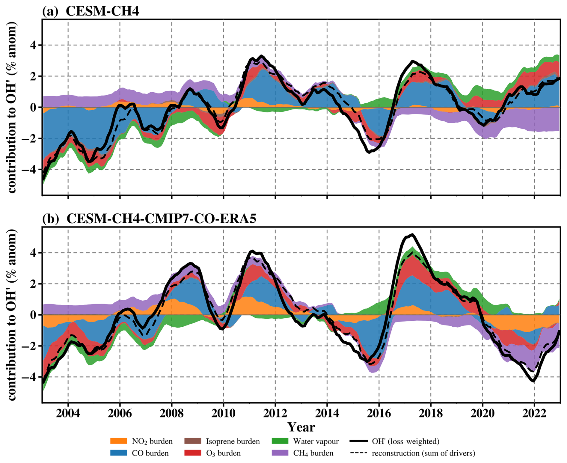
Figure 16 Driver contributions to the global, loss-weighted OH anomaly in the burden basis (the CO, NO₂, O₃, isoprene and CH₄ burdens and water vapour), for (a) CESM-CH4 and (b) CESM-CH4-CMIP7-CO-ERA5. Bands are the stacked per-driver contributions (% anomaly); the black line is OH^′ and the dashed line its reconstruction (the sum of the coloured bands).

As quantified in Sect. 5, the OH-driven contribution to the 2020 growth is moderate in comparison to several studies in the literature. In CESM-CH4-CMIP7-CO-ERA5, the NO+HO₂ source is lower in 2020 and even lower in 2021–2022 (Figs. 14d, 15b), likely driven by the CMIP7 emissions taking into account the lockdown effect and a slow rebound in emissions during these years. It is accompanied by a lower O₃ and subsequent reduced O(¹D)+H₂O. It shows a simultaneous decline in the surface NO_x forcing, in agreement with the COVID-19 emission reductions (Gaubert et al., 2021; Miyazaki et al., 2021). In addition to reduced anthropogenic precursor emissions, the exceptionally strong and persistent Arctic polar vortex in winter–spring 2020, which produced record-low lower stratospheric O₃, reduced stratosphere-to-troposphere transport of O₃ and contributed to the negative tropospheric O₃ anomalies observed in spring 2020 (Bouarar et al., 2021). These negative terms are partly offset by positive anthropogenic and fire CO terms, despite an extended fire season that started with the Australian fires (Chen et al., 2025), but was also larger than usual during the boreal summer (Ortega et al., 2023), and over the Amazon (Libonati et al., 2021). Because these emission predictors are correlated (Figs. S14 and S15), their individual contributions can have larger uncertainties and are better interpreted as a combined emission contribution. We also find a conflicting but interesting role of meteorologically driven anomalies of lightning NO_x, with a negative anomaly in ERA5 driven simulation after 2020, as discussed earlier (Fig. 15b). Under CESM-CH4-CMIP7-CO-ERA5 the convective lightning source does not offset the surface-NO_x reduction as it does under CESM-CH4 (MERRA-2), so the NO_x-recycling pathway is reduced, whereas in CESM-CH4, sources and sinks are balanced and there is a low OH interannual variability. In CESM-CH4, while the COVID-19 effect is included, it has a smaller impact and the anomalies are smaller for most fluxes. As for 2015, both simulations show elevated biogenic isoprene that consumes OH and suppresses ozone (in the absence of NO_x), in line with a recent study using CrIS isoprene data (Yoon et al., 2025) or the idealized aquaplanet version of CAM-chem (Aqua-chem, Zhu et al., 2026). The simulations diverge decisively after 2020, when the OH in CESM-CH4 stays mildly positive while that in CESM-CH4-CMIP7-CO-ERA5 plunges with continued lower lightning emissions. There are also important differences with reduced surface anthropogenic NO_x in CMIP7 emissions, which do not recover after 2020, and different biomass-burning emissions emerging in the fire-CO terms, most notably in 2021 and 2022 (Fig. 15b). This lower OH in the CESM-CH4-CMIP7-CO-ERA5 simulations drives the higher CH₄ growth rate during these years (Sect. 5).

Finally, to assess the influence of the El Niño–Southern Oscillation (ENSO) on OH variability, we correlated the loss-weighted OH anomaly with the MEI.v2 index (Wolter and Timlin, 2011). In the sink-controlled CESM-CH4 simulation, OH is significantly anti-correlated with ENSO (annual $r=-\mathrm{0.63}$, p=0.01), with lower OH during El Niño conditions and higher OH during La Niña. Monthly cross-correlation analysis shows the strongest relationship when ENSO lags OH by approximately 2–4 months. The CO burden behaves consistently, showing a positive correlation with ENSO ($r=+\mathrm{0.40}$ with MEI.v2) and a negative correlation with OH (Fig. S11). These results are consistent with methyl chloroform constraints reported by Patra et al. (2021), who found the CH₄ loss rate to be anti-correlated with the same ENSO index ($r=-\mathrm{0.29}$ to −0.38, with lags of 3–8 months), although the simulated response in CESM-CH4 is stronger. In the OH production-controlled CESM-CH4-CMIP7-CO-ERA5 simulation, the correlation weakens substantially ($r=-\mathrm{0.25}$), indicating that variability in lightning NO_x (and related O₃-driven) OH production partially offsets the ENSO-driven sink response. An example occurs during 2020–2022, when OH decreases despite persistent La Niña conditions that would otherwise favour higher OH. Because of buffering impact with interactive OH, its impact on CH₄ growth rate is at most about one-fifth of the 2020–2022 CH₄ growth rate anomaly in the two best experiments, which is substantially smaller than the ∼ 80 % contribution inferred from prescribed-OH inversions (Ciais et al., 2026). Future work should focus on better quantifying the regional to continental differences in OH that are driven by ENSO (Shutter et al., 2024).

7 Conclusions

We summarize the findings of this study as follows:

1. The CH₄+OH reaction is estimated to contribute about 13 % of the OH loss, here calculated for the year 2013. Since the CH₄ burden evolves slowly, we conclude that the CH₄ contribution to the interannual OH variability is small. This is illustrated in two pairs of simulation experiments. In a simulation in which CH₄ emissions were kept at 2003 levels throughout our 20-year period, the average OH was only reduced by 0.4 %. We compared one emission- and one concentration-driven simulation, which had a similar CH₄ burden, but with a different spatial and temporal distribution. They showed no differences in annual and global CH₄ chemical lifetime with respect to tropospheric OH. This suggests that emission-driven CH₄ simulations are not needed when the goal is to study OH and chemistry only. This also questions the estimation of OH from CH₄ inversions since CH₄ provides very little information on the OH interannual variability. Early benefits of estimating OH might have come from reducing the OH prior bias (Penn et al., 2025).

2. Saunois et al. (2025) indicate that uncertainty due to the chemical loss of CH₄ by OH from atmospheric chemistry models is around 15 %–20 %. Here we show it is possible to simulate an OH field with an uncertainty similar to the one estimated by methyl-chloroform inversions (i.e., 10 %). The two best simulations differ by about 1 % from the scaled OH of Spivakovsky et al. (2000). However, the simulated OH remains higher in the NH than in the SH.

3. In contrast, using established emission inventories (CAMS/FINN2.5 vs. CEDS-CMIP7) with different spatial distributions, chemical speciation, and temporal variation led to a net 10 % difference in OH between simulations on average during the 2003–2022 period. This resulted in an 8 % shorter CH₄ lifetime in the CMIP7 configuration, which caused a strong bias in simulated CH₄. Tropical fire emissions play an important role by increasing both sources and sinks of OH, here because of higher emission from FINN2.5, and therefore the CO and CH₄ global budget. From both simulations, the fire emissions impact the OH interannual variability and trends.

4. This study presents the first comparison of nudging the CAM-chem model to the hourly ERA5 reanalysis dataset. The switch from the MERRA-2 3-hourly dataset has a comparable impact in magnitude on OH levels to the complete anthropogenic and fire emission inventory swap. The CH₄ lifetime is increased by 9.3 % when using ERA5 due to stronger biogenic emissions. Despite the pair of simulations using the same set of emissions, the CH₄ chemical loss is reduced by 20 Tg CH₄ yr⁻¹ and the atmospheric growth rate is increased from around 10 to 23 Tg CH₄ yr⁻¹. In this case, the simulation nudged to ERA5 is much closer to the observed growth rate. On average, the impact of meteorology on OH results from offsets in vegetation emissions, as estimated by the MEGAN model, which are strongly sensitive to temperature and radiation. These biogenic emissions have a large impact through a cascade of reactions involving isoprene and other organic compounds that effectively reduce OH and ultimately increase CO. There is a clear recycling of OH through increased VOCs and H₂O₂ sources of OH. Satellite observations of isoprene (Wells et al., 2020) have the potential to constrain the magnitude as well as the temporal and spatial distribution of the isoprene emissions (Choi et al., 2025; Li et al., 2025; Yoon et al., 2025, 2026). However, these top-down estimates currently diverge, even for the global and annual total fluxes, and some, including ours, tend to be higher than a bottom-up dataset (Sindelarova et al., 2022). Regarding CESM, future work should focus on the integration of an improved organic chemistry mechanism (TS2) for isoprene and monoterpenes (Schwantes et al., 2020; Mirrezaei et al., 2026b) with the SLH updates used here.

5. We find that the two reanalysis datasets produce a strong difference in lightning NO_x emissions over the 2020–2022 period, resulting in large uncertainties in CH₄ lifetime anomalies. Previous studies have shown that meteorological nudging affects mean OH concentrations rather than OH interannual variability or decadal trends (Gaubert et al., 2017; He et al., 2021). Our results suggest that reanalysis-dependent differences in lightning NO_x emissions can nevertheless introduce substantial uncertainty in OH and CH₄ lifetime anomalies during specific periods. To better constrain which reanalysis dataset represents these processes more realistically, future work will focus on evaluating how key parameterizations (e.g., convection, biogenic emissions) respond to nudging. Future work should be dedicated to updating the parameterization, with guidance from the recent literature (Dang et al., 2026; Pickering et al., 2026). We will evaluate these simulations against independent observational datasets such as aircraft field campaigns and satellite observations.

6. Because the two best configurations share the same CH₄ emissions, their OH difference imprints directly on the year-to-year growth rate, and the OH-driven contribution to the 2020–2022 surge spans from near zero (MERRA-2) to about one fifth of the growth (ERA5). While the ERA5 run reproduces the overall elevated CH₄ growth better, the year-by-year comparison with NOAA GML measurements suggests that its OH reduction may be somewhat too strong in the peak years of 2020–2022, or that the posterior CH₄ emissions used here (CT-CH4-2025) are overestimated.

7. The interannual OH variability is governed by different contributions: the CESM-CH4 run shows larger sensitivity to the CO burden controlling the OH sink, while the ERA5 run is more sensitive to the production of OH from the O(¹D)+H₂O and NO_x sources. The two simulations therefore agree when an ENSO-paced swing in emissions of fire CO, biogenic NMVOCs and lightning NO_x dominates (2011, 2015) and diverge when meteorology varies (2016–2017 and, most strongly, 2020–2022). The loss-weighted regional regressions indicate that OH variability is associated mainly with surface NO_x, CO, isoprene and lightning NO_x, while the CH₄ emission predictors add little explanatory power once the other drivers are included. Because the drivers co-vary, these associations are interpreted alongside the diagnosed OH production and loss pathways rather than as an exact partition of individual physical effects.

8. For 2020, the two simulations attribute an OH-driven CH₄ forcing of +1.4 ppb yr⁻¹ (≈4 Tg yr⁻¹; about 12 % of the emission-plus-OH forcing ΔE−m Δk) in CESM-CH4 and +4.8 ppb yr⁻¹ (≈13 Tg yr⁻¹; about 31 %) in CESM-CH4-CMIP7-CO-ERA5. The CESM-CH4 estimate is close to the 5 Tg yr⁻¹ (14 %) reported by Qu et al. (2022), but lower than other studies that quantify an impact of OH closer to 50 % (Stevenson et al., 2022; Peng et al., 2022; Chen et al., 2025; Brasseur and Gaubert, 2025).

9. During our 20-year study period, tropospheric OH reached its largest positive anomalies (more than 3 %) in 2011 and 2017, associated with lower biogenic emissions, higher lightning NO_x, and lower fire CO emissions. Because the OH forcing on the growth rate depends on the year-to-year change in OH rather than its absolute level, the largest OH-driven reductions in the CH₄ growth rate occur when OH rose most steeply, about 4 ppb yr⁻¹ during the 2011 increase and up to 7 ppb yr⁻¹ in 2016, as OH climbed toward the 2017 maximum. Both exceeded the 2020 OH contribution. Conversely, 2015 stands out as a low-OH year, during the 2015–2016 El Niño, in which weaker oxidation raised the CH₄ growth rate.

10. The absence of significant OH trends over 2003–2022 is robust across CESM-CH4 and CESM-CH4-CMIP7-CO-ERA5 simulations, demonstrating consistency despite differences in meteorology and emissions.

This study highlights that further work is needed to reduce OH uncertainties, which will be critical for improving estimates of the CH₄ budget, but also for the Earth's tropospheric chemistry system as a whole. This can be achieved by an improved understanding of tropospheric chemistry and OH reactivity (Travis et al., 2020; Fuchs et al., 2025; Price et al., 2025; Tan et al., 2026), a better characterization (Strode et al., 2026; Nicely et al., 2018) and uncertainty quantification (Murray et al., 2021; Wild and Ryan, 2026) of the OH drivers across models, as well as innovative use of multiple satellite observations (Duncan et al., 2024; Anderson et al., 2022; Souri et al., 2024; Shutter et al., 2024). Our improved modelling framework is also well suited to assess the direct and indirect effects of molecular hydrogen (H₂) on OH, and hence on the CH₄ budget (Bryant and Stevenson, 2024; Yang et al., 2025; Chua et al., 2025), an effect of growing importance as the hydrogen economy expands. Finally, a model intercomparison project for methane emission-driven simulations with interactive atmospheric chemistry is essential to quantify the spread in tropospheric oxidant feedbacks, improved OH and short-lived halogen chemistry representations, and methane lifetime estimates across Earth system models.

We find that OH is well buffered against chemistry perturbations, as increased chemical complexity raises the OH recycling probability. Consequently, studies relying on simplified and prescribed OH representations may neglect these complex chemical feedbacks and overestimate the role of OH changes in driving the CH₄ growth rate. In line with previous studies (Skeie et al., 2023), the atmospheric CH₄ growth rate is mainly controlled by direct CH₄ emissions, which should be the focus of mitigation for climate targets (Shindell et al., 2024).

Appendix A: Chemistry updates

The methyl peroxy radical (CH₃O₂) reaction with OH has been proposed to be important by Archibald et al. (2009) and has been implemented in global models (e.g., Bates et al., 2021). Assaf et al. (2017) performed laboratory measurements and identified that previous yield of methanol of up to 30 % from (Müller et al., 2016) and the reaction rate (Bossolasco et al., 2014) were likely overestimated. Here, we calculate the average of the reaction rate between Yan et al. (2016) and Assaf et al. (2017) and we obtain $k=\mathrm{1.2}\times {\mathrm{10}}^{-\mathrm{10}}$ cm³ molecule⁻¹ s⁻¹. Assuming the alkoxy (CH₃O) intermediate reacts rapidly with O₂ to produce formaldehyde and HO₂, and (for simplicity) redistributing the CH₃OOOH adduct product between CH₃OH and CH₂O, we obtain:

$$\begin{array}{}\text{(AR1)}& \begin{array}{rl}{\mathrm{CH}}_{\mathrm{3}}{\mathrm{O}}_{\mathrm{2}}& +\mathrm{OH}+\mathrm{0.89}\cdot {\mathrm{O}}_{\mathrm{2}}\to \mathrm{0.11}\cdot {\mathrm{CH}}_{\mathrm{3}}\mathrm{OH}\\ & +\mathrm{0.11}\cdot {\mathrm{O}}_{\mathrm{2}}+\mathrm{1.78}\cdot {\mathrm{HO}}_{\mathrm{2}}+\mathrm{0.89}\cdot {\mathrm{CH}}_{\mathrm{2}}\mathrm{O};\\ & k=\mathrm{1.2}\times {\mathrm{10}}^{-\mathrm{10}}{\mathrm{cm}}^{\mathrm{3}}{\mathrm{molecule}}^{-\mathrm{1}}{\mathrm{s}}^{-\mathrm{1}}\end{array}\end{array}$$

Our low yield of 11 % of CH₃OH is closer to the GEOS-Chem implementation of 13 % from Bates et al. (2021).