Vertical profiling and aerosol typing using fluorescence Raman and depolarization lidar measurements over Thessaloniki, Greece

In this study, we present the first fluorescence lidar observations over Thessaloniki, Greece, (40.63° N, 22.96° E; 60 m a.s.l.) using a multiwavelength Raman and depolarization lidar with fluorescence capabilities. For the first time in the Eastern Mediterranean fluorescence backscattering coefficient and the spectral fluorescence capacity parameter are retrieved and combined with particle depolarization ratio, lidar ratios, and Ångström exponents to characterize the aerosol load over Thessaloniki, a region influenced by diverse aerosol sources. Representative case studies of biomass-burning smoke, Saharan dust, and mixed pollen showing distinct fluorescence properties are discussed in detail, while an extended dataset covering the period April 2024–December 2025 is further analysed, comprising 108 aerosol layers from 50 measurement cases. A sub-dataset is also compared with the EARLINET Mahalanobis distance–based typing algorithm, highlighting the importance and complementarity of fluorescence lidar observations on the aerosol characterization in complex environments. Based on the spectral fluorescence capacity and the particle depolarization ratio, the identified layers are classified into smoke, dust, polluted continental, clean continental and mixed pollen. THELISYS retrievals show that the spectral fluorescence capacity depends on aerosol type, with smoke showing the highest values ($\mathrm{3.5}\times {\mathrm{10}}^{-\mathrm{6}}-\mathrm{12.7}\times {\mathrm{10}}^{-\mathrm{6}}$ nm⁻¹), followed by mixed pollen ($\mathrm{2.3}\times {\mathrm{10}}^{-\mathrm{6}}-\mathrm{4.8}\times {\mathrm{10}}^{-\mathrm{6}}$ nm⁻¹), polluted continental ($\mathrm{1.0}\times {\mathrm{10}}^{-\mathrm{6}}-\mathrm{3.3}\times {\mathrm{10}}^{-\mathrm{6}}$ nm⁻¹), clean continental ($\mathrm{0.3}\times {\mathrm{10}}^{-\mathrm{6}}-\mathrm{1.2}\times {\mathrm{10}}^{-\mathrm{6}}$ nm⁻¹) and dust ($\mathrm{0.4}\times {\mathrm{10}}^{-\mathrm{6}}-\mathrm{1.3}\times {\mathrm{10}}^{-\mathrm{6}}$ nm⁻¹). The fluorescence capacity values observed for all aerosol types are comparable with other studies across central and northern Europe, however the linear particle depolarization ratio measurements attributed to pollen differ from those reported at more northern latitudes, possibly reflecting differences in pollen type.

1 Introduction

Atmospheric aerosols play a crucial role in Earth's climate system, air quality, and public health. Conventional lidar techniques, including elastic backscatter, Raman, depolarization, and high-spectral-resolution lidar (HSRL), provide information on aerosol optical properties, shape, size distributions, and concentrations (Klett, 1981; Fernald, 1984; Ansmann et al., 1990; Sassen, 2005; Whiteman, 2003; Burton et al., 2015). However, these methods lack the sensitivity required for reliable discrimination among biologically derived particles. Over the past decade, fluorescence lidar has emerged as a powerful complementary technique, enabling the detection of biochemical constituents and fluorescence properties of aerosols and thereby enhancing aerosol classification capabilities.

Early applications of fluorescence lidar were primarily focused on environmental monitoring, including vegetation characterization, water quality assessment, and geosphere studies, as summarized by Saito et al. (2018). Since approximately 2014, fluorescence lidar has increasingly been applied to atmospheric research. Two principal approaches for aerosol fluorescence retrieval have been established, the spectrometric fluorescence lidar and the single channel fluorescence detection implemented within Mie-Raman lidar systems.

In the context of aerosol fluorescence spectroscopy, Reichardt (2014) integrated a multi-channel fluorescence spectrometer into a standard Raman lidar system, enabling the first quantitative retrievals of aerosol fluorescence. This methodology was subsequently refined through improved calibration and retrieval techniques (Reichardt et al., 2023) and extended to a multi-year dataset (2020–2023) that could only be obtained by spectrometric measurements (Reichardt et al., 2025). A key outcome of these studies was the introduction of the spectrum of fluorescence capacity and the connections between aerosol fluorescence and other parameters and influencing factors, such as the elastic-optical particle properties, the type and origin of the aerosols, the atmospheric state variables, and clouds.

In parallel, Veselovskii et al. (2020) extended the operational capabilities of lidar systems compatible with the Aerosol, Clouds and Trace Gases Research Infrastructure (ACTRIS; https://www.actris.eu/, last access: 20 September 2026) Aerosol Remote Sensing requirements (CARS; https://www.actris.eu/topical-centre/cars, last access: 20 September 2026). These requirements include lidar systems equipped with at least one-wavelength Raman or High-Spectral-Resolution (HSR) lidar with polarization discrimination, combined with an automatic sun/sky photometer, to which an additional broadband channel can be readily added. Their approach involved the integration of a single broadband fluorescence channel centered at 466 nm into the multiwavelength Mie–Raman lidar system LILAS (Lille Lidar for Atmospheric Study). Initial feasibility studies conducted between 2018 and 2020 demonstrated that even a single fluorescence channel allows for the retrieval of fluorescence backscattering coefficients and the derivation of an intensive fluorescence capacity parameter.

The standardisation of quantitative particle fluorescence retrievals into operational lidar systems represents a major challenge in aerosol classification using remote sensing. By combining fluorescence capacity with particle depolarization ratio, intensive aerosol classification has been achieved (Veselovskii et al., 2022b, 2025; Miri et al., 2025). Veselovskii et al. (2021, 2022a, 2023) demonstrated discrimination among pollen, biomass-burning smoke, mineral dust, urban aerosols, and cirrus clouds with high spatial and temporal resolution. These studies conducted over Lille revealed that smoke layers transported from North America exhibited fluorescence capacities up to an order of magnitude higher than urban aerosols, while Saharan dust was characterized by low fluorescence capacity but high depolarization ratios. Pollen events were identified by concurrent enhancements in both depolarization and fluorescence capacity, frequently forming mixed layers with urban aerosols within the planetary boundary layer. Furthermore, Hu et al. (2022) extended this methodology to complex atmospheric scenarios involving overlapping smoke and cirrus layers, demonstrating that fluorescence based classification remains useful even under cloud-contaminated conditions. More recently, Gast et al. (2025) validated the general applicability of this approach by demonstrating consistent aerosol classification across different lidar systems and geographic regions.

Collectively, these studies demonstrate that fluorescence based aerosol classification enhances aerosol typing, particularly under conditions where traditional multiwavelength Mie–Raman approaches encounter limitations. This capability provides a powerful tool for atmospheric monitoring and for advancing the understanding of aerosol–cloud interactions (Reichardt, 2014; Reichardt et al., 2018). In this context, aerosol typing over Thessaloniki during the period 2024–2025 represents a particularly valuable case study. Thessaloniki is a densely populated urban site in the Eastern Mediterranean, where mineral dust, biomass-burning smoke, anthropogenic pollution, pollen and marine aerosols frequently coexist, rendering it an ideal location for evaluating and refining aerosol classification methodologies (Voudouri et al., 2020).

Beyond mineral and anthropogenic particles, biological aerosols, especially pollen, constitute a significant yet still insufficiently characterized fraction of atmospheric aerosols. Extensive research has investigated various aspects of airborne pollen in Thessaloniki (Papadogiannaki et al., 2025; Vokou et al., 2024; Charalampopoulos et al., 2021). Based on long-term observations of 16 pollen taxa, the local pollen spectrum is dominated by Cupressaceae (24.9 %), Quercus (20.8 %), Parietaria (13.6 %), Olea (9.1 %), Pinaceae (8.9 %), and Poaceae (6.3 %) (Gioulekas et al., 2004). Building on these findings, Damialis et al. (2007) analysed long-term pollen trends (1987–2005), revealing a general doubling of airborne pollen concentrations per decade across several taxa. Furthermore, they conducted one of the few vertical profiling studies in the region using ground based and airborne platforms, confirming the presence of pollen – particularly Pinaceae and Quercus – at altitudes up to 2 km above ground level. These observations indicate that pollen grains can remain airborne for extended periods and undergo long-range transport, thereby expanding the spatial scale of human exposure. Such findings underscore the need for continuous, high-resolution vertical profiling techniques. In this regard, fluorescence lidar provides a unique capability for investigating the vertical distribution of pollen by exploiting their intrinsic fluorescent properties to distinguish biological from non-biological aerosols.

Within this framework, the present study reports, for the first time, vertical measurements of aerosol and pollen over Thessaloniki during 2024–2025, using fluorescence lidar observations in a complex urban Mediterranean environment. The paper is organized as follows: Sect. 2 describes the lidar system and the analysis methodology, including system configuration, data pre-processing, and fluorescence retrieval techniques with different interference filters (IF). Section 3 presents and discusses the results of three case studies and the classification scheme based on fluorescence capacity and particle depolarization ratio, while Sect. 4 summarizes the main conclusions of the study.

2 Instrument and methods

2.1 Thessaloniki's lidar system upgrade

Thessaloniki's lidar system (THELISYS) is part of the multitype ground-based instruments that belong to the Laboratory of Atmospheric Physics (LAP), located in the Physics Department of the Aristotle University of Thessaloniki (AUTH), Greece (40.63° N, 22.96° E; 60 m a.s.l.) and is part of the European Aerosol Research Lidar Network (EARLINET: https://www.earlinet.org/, last access: 10 October 2026). Quality assurance procedures for lidar signals are guaranteed using the Automated Lidar Analysis Software (ATLAS; https://github.com/nikolaos-siomos/ATLAS, last access: 10 October 2026) passing all the quality assurance standards established within EARLINET (Freudenthaler et al., 2018), providing quality assured aerosol products.

THELISYS lidar has been gradually upgraded since 2021, to be fully automated, providing continuous measurements of aerosol and cirrus cloud properties in the frame of the project “Panhellenic infrastructure for Atmospheric Composition and climate change” (PANACEA; https://panacea-ri.gr, , last access: 10 September 2025). More details about the THELISYS setups through the last decades can be found in previous studies (Siomos et al., 2018; Voudouri et al., 2020; Michailidis, 2023).

THELISYS is a $\mathrm{3}\mathit{\beta }+\mathrm{2}\mathit{\alpha }+\mathrm{1}\mathit{\delta }+\mathrm{1}\mathrm{WV}+\mathrm{1}$G lidar system that retrieves the aerosol backscatter coefficient (β_aer) at 3 wavelengths (355, 532, 1064 nm), the aerosol fluorescence backscatter coefficient (β_F) at 466 nm (since February 2025), the aerosol extinction coefficient (α_aer) at 2 wavelengths (355, 532 nm), alongside aerosol extensive and intensive properties such as backscatter- and extinction-related Ångström exponents (BAE${}_{\mathrm{355}/\mathrm{532}}$, EAE${}_{\mathrm{355}/\mathrm{532}}$, BAE${}_{\mathrm{532}/\mathrm{1064}}$), lidar ratio (LR_532,LR₃₅₅), volume and particle linear depolarization ratio (VLDR₅₃₂, PLDR₅₃₂), water vapor mixing ratio (MR₄₀₈) and fluorescence capacity (G_F). All collected signals undergo processing for the retrieval of the lidar profiles using the Single Calculus Chain (SCC; D'Amico et al., 2015) algorithm, the fully automated algorithm, which has been developed to provide a common lidar processing tool, within EARLINET stations. However, SCC in its current version does not handle water vapor and fluorescence channels so for the new products the signals undergo processing using the in-house Semi-automated multiwavelength Lidar Algorithm (SULA; Paschou et al., 2022) developed by the National Observatory of Athens (NOA) with contribution from AUTH on the water vapor and fluorescence retrievals.

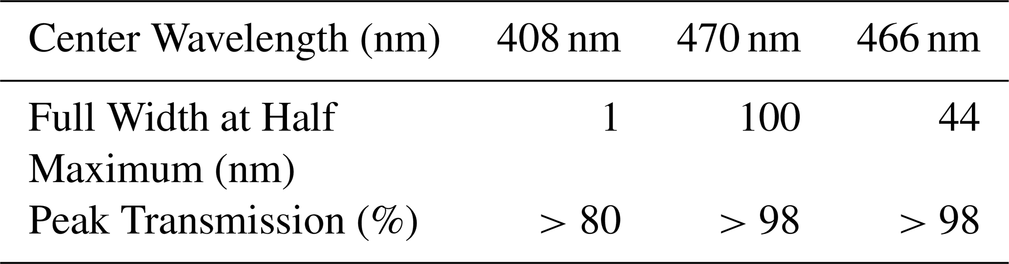
More specifically about the latest upgrades, in June 2023, THELISYS was equipped with a single dual-use channel, one centered at 470 nm for deriving the aerosol fluorescence capacity similar with the lidar system LIF (lidar Laser Induced Fluorescence; Gidarakou et al., 2026) and the other one centered at 408 nm for deriving the water vapor mixing ratio profile using appropriate IFs. In February 2025, the IF centered at 470 nm with full width at half maximum (FWHM) of 100 nm in the fluorescence channel was replaced by an IF at 466 nm with 44 nm FWHM, in order to ensure comparability with lidar systems operating in Lille (Veselovskii et al., 2021) and Leipzig (Gast et al., 2025). Differences in retrievals arising from the use of different filters can be adjusted as described in Sect. 2.3. The two IF are resided in a single photomultiplier tube (PMT) that employs a motorized shutter to insert the appropriate IF whenever we intend to acquire water vapor or fluorescence measurements. The technical characteristics of the IF are presented in Table 1.

Table 1 Technical characteristics of the optical components for the water vapor and fluorescence interference filters of THELISYS.

2.1.1 Fluorescence measurements and analysis

In this study, the aerosol fluorescence backscatter coefficient and fluorescence capacity were retrieved using the method described by Veselovskii et al. (2020). The method relies on the fluorescence signal P_F and the nitrogen Raman signal P_R, which are described by the following equations:

$$\begin{array}{}\text{(1)}& {\displaystyle }{P}_{\mathrm{F}}\left(z\right)=C_{\mathrm{F}}{\mathit{\beta }}_{\mathrm{F}}\left(z\right)T_{\mathrm{L}}\left(z\right)T_{\mathrm{F}}\left(z\right)\text{(2)}& {\displaystyle }{P}_{\mathrm{R}}\left(z\right)=C_{\mathrm{R}}{\mathit{\beta }}_{\mathrm{R}}\left(z\right)T_{\mathrm{L}}\left(z\right)T_{\mathrm{R}}\left(z\right),\end{array}$$

where C represents the calibration constants, β the backscatter coefficients and T the atmospheric transmission terms. The subscripts F, R and L denote fluorescence, nitrogen Raman and elastic scattering, respectively.

The ratio of the Eq. (1) to the Eq. (2) is used to obtain the aerosol fluorescence backscatter coefficient β_F(z):

$$\begin{array}{}\text{(3)}& {\mathit{\beta }}_{\mathrm{F}}\left(z\right)={\displaystyle \frac{C_{\mathrm{R}}}{C_{\mathrm{F}}}}{\displaystyle \frac{P_{\mathrm{F}}\left(z\right)}{P_{\mathrm{R}}\left(z\right)}}{N}_{\mathrm{R}}\left(z\right){\mathit{\sigma }}_{\mathrm{R}}{\displaystyle \frac{T_{\mathrm{R}}\left(z\right)}{T_{\mathrm{F}}\left(z\right)}},\end{array}$$

where ${\mathit{\sigma }}_{\mathrm{R}}=\mathrm{2.744}\times {\mathrm{10}}^{-\mathrm{30}}$ cm² sr⁻¹ (Venable et al., 2011) is the vibrational-rotational Raman differential backscattering cross section of molecular nitrogen at 355 nm and the number density of nitrogen is given by the relation:

$$\begin{array}{}\text{(4)}& N_{\mathrm{R}}\left(z\right)=c_{{\mathrm{N}}_{\mathrm{2}}}{N}_{\mathrm{mol}}\left(z\right)=\mathrm{0.78}{N}_{\mathrm{mol}},\end{array}$$

where $c_{{\mathrm{N}}_{\mathrm{2}}}$ is the volume fraction of nitrogen in air and N_mol is the molecular number density of air for a given temperature and pressure, considering the compressibility of air. The ratio $T_{\mathrm{R}}\left(z\right)/T_{\mathrm{F}}\left(z\right)$ of the atmospheric transmissions at the Raman and fluorescence wavelengths is calculated from the extinction coefficients at the corresponding wavelengths applying the related extinction Ångström exponent correlation, ${\mathrm{EAE}}_{\mathrm{355}/\mathrm{532}}$ (Ansmann et al., 1990). The calibration constants C_F and C_R are range-independent system constants accounting for the overall optical and electronic response of the fluorescence and Raman detection channels, respectively. The calibration factors ratio $C_{\mathrm{R}}/C_{\mathrm{F}}$ therefore represents the relative calibration factor between the Raman and fluorescence channels; it corrects for their different instrumental efficiencies and is calculated following the calibration procedure described by Veselovskii et al. (2020) and analysed by Gast et al. (2025). This procedure is based on the ratio of the electronic gains of the PMTs and considers each component in the respective detection path of the two channels, as described above, thus the calibration factor is given by the relationship:

$$\begin{array}{}\text{(5)}& {\displaystyle \frac{C_{\mathrm{R}}}{C_{\mathrm{F}}}}={\displaystyle \frac{g_{\mathrm{R}}}{g_{\mathrm{F}}}}{\displaystyle \frac{T_{\mathrm{IF},\mathrm{R}}}{T_{\mathrm{IF},\mathrm{F}}}}.\end{array}$$

The electronic gain (g) was obtained by exchanging the PMTs of the two channels without changing the IF and calculating the ratio of the mean signals measured by both PMTs for the fluorescence or the Raman channel. The test produced a PMT gain ratio ($g_{\mathrm{R}}/g_{\mathrm{F}}$) of 1.63. Considering the transmission of the different IFs of the channels ($T_{\mathrm{IF},\mathrm{R}}/T_{\mathrm{IF},\mathrm{F}}\sim \mathrm{0.75})$ one obtains a value of ∼1.59 for $C_{\mathrm{R}}/C_{\mathrm{F}}$, the ratio of the calibration factors.

Once the fluorescence backscatter coefficient is derived, the fluorescence capacity G_F can be calculated using the ratio of the fluorescence backscatter to the aerosol backscatter coefficient at 532 nm retrieved with the Raman backscatter method (Ferrare et al., 1998):

$$\begin{array}{}\text{(6)}& G_{\mathrm{F}}={\displaystyle \frac{{\mathit{\beta }}_{\mathrm{F}}}{{\mathit{\beta }}_{\mathrm{532}}}}.\end{array}$$

Although fluorescence is excited at 355 nm and it would therefore be preferable to use the aerosol backscatter coefficient at the same wavelength (β₃₅₅), the elastic aerosol backscatter coefficient at 532 nm is used here in order to enable comparison with existing literature.

For improved intercomparison with other fluorescence lidar configurations, particularly lidar systems employing broadband fluorescence channels with varying filter widths or spectrometers, we convert the retrieved fluorescence capacity to a spectral quantity. The spectral fluorescence capacity $G_{\mathrm{F}}^{\mathrm{355}}$ is calculated according to Gast et al. (2025) as

$$\begin{array}{}\text{(7)}& G_{\mathrm{F}}^{\mathrm{355}}={\displaystyle \frac{{\mathit{\beta }}_{\mathrm{F}}}{{\mathit{\beta }}_{\mathrm{355}}{d}_{\mathrm{IF}}}},\end{array}$$

with d_IF representing the effective bandwidth of the fluorescence IF. Both spectral fluorescence capacity ($G_{\mathrm{F}}^{\mathrm{355}}$) and fluorescence capacity (G_F) are presented in the results below to allow comparison with the existing literature. In the text, G_F is given in parentheses.

2.1.2 Comparison of different fluorescence interference filters

In lidar instruments that deploy broadband fluorescence channels, the characteristics of the IFs that are being used, such as the central wavelength and the FWHM, are selected according to the fluorescence emission spectrum of the fluorescing particles of interest. The particle fluorescence spectrum depends both on the excitation laser line (here 355 nm) and on the particle chemical composition and mixing state. For an excitation with the 355 (more precisely 354.71 nm) line, an IF with central wavelength between 466 to 470 nm and bandwidths ranging up to 100 nm has been preferred for broadband fluorescence applications. Although not necessarily located at the maximum of the fluorescence spectrum, the spectral region 415–525 nm avoids contamination of other major Nd:Yag-related and Raman lines such as the water vapor Raman line at 408 nm and the 2nd Nd:Yag laser harmonic at 532 nm and its Anti-Stokes purely rotational Raman band. In THELISYS, an IF centered at 469.55 nm (approximately 470 nm) with 100 nm FWHM was initially deployed to isolate part of the fluorescence spectrum. However, differences in the IF transmission hindered direct comparison with fluorescence measurements performed in Lille (Veselovskii et al., 2021) and Leipzig (Gast et al., 2025). In addition, Reichardt et al. (2023) and Veselovskii et al. (2023) reported that the 424.4 nm second-order vibrational Raman line of N₂ can introduce biases to the fluorescence spectrum (Reichardt et al., 2023). To improve the consistency of THELISYS lidar with the lidars in Lille and Leipzig, the IF at 470 nm was replaced by an IF with transmission centered at 465.73 nm (approximately 466 nm) and with 44 nm FWHM. We will refer to those filters as IF_470,100 and IF_466,44 respectively.

The mean $G_{\mathrm{F}}^{\mathrm{355}}$ calculated using such a broad IF will differ from the actual $G_{\mathrm{F}}^{\mathrm{355}}$ at the IF center wavelengths. Using the $G_{\mathrm{F}}^{\mathrm{355}}$ spectrum measured by Reichardt et al. (2025) as a reference (Fig. 1) we can estimate the systematic relative bias ${\mathit{\sigma }}_{G_{\mathrm{F}},{\mathrm{IF}}_{\mathrm{466}}}$ and ${\mathit{\sigma }}_{G_{\mathrm{F}},{\mathrm{IF}}_{\mathrm{470}}}$ of $G_{\mathrm{F},\mathrm{466}}^{\mathrm{355}}$ and $G_{\mathrm{F},\mathrm{470}}^{\mathrm{355}}$ which are introduced when using IF_466,44 and IF_470,100, respectively, as

$$\begin{array}{}\text{(8)}& {\mathit{\sigma }}_{G_{\mathrm{F}},{\mathrm{IF}}_{{\mathit{\lambda }}_{\mathrm{0}}}}={\displaystyle \frac{\stackrel{\mathrm{‾}}{G_{\mathrm{F},{\mathit{\lambda }}_{\mathrm{IF}}}^{\mathrm{355}}}-G_{\mathrm{F},{\mathit{\lambda }}_{\mathrm{0}}}^{\mathrm{355}}}{G_{\mathrm{F},{\mathit{\lambda }}_{\mathrm{0}}}^{\mathrm{355}}}},\end{array}$$

where $G_{\mathrm{F},{\mathit{\lambda }}_{\mathrm{0}}}^{\mathrm{355}}$ the spectral fluorescence capacity at λ₀=466 or 470 nm and $\stackrel{\mathrm{‾}}{G_{\mathrm{F},{\mathit{\lambda }}_{\mathrm{IF}}}^{\mathrm{355}}}$ is the spectral fluorescence weighted mean signal. The latter is calculated using the filter transmission as weighting function:

$$\begin{array}{}\text{(9)}& \stackrel{\mathrm{‾}}{G_{\mathrm{F},{\mathit{\lambda }}_{\mathrm{IF}}}^{\mathrm{355}}}={\displaystyle \frac{\int G_{\mathrm{F}}^{\mathrm{355}}\left(\mathit{\lambda }\right)\times T_{\mathrm{IF}}\left(\mathit{\lambda }\right)\mathrm{d}\mathit{\lambda }}{\int T_{\mathrm{IF}}\left(\mathit{\lambda }\right)\mathrm{d}\mathit{\lambda }}}.\end{array}$$

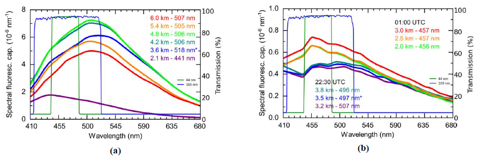
Figure 1 Spectral fluorescence capacity measurements of a biomass burning aerosol layer at 22:30 UTC on 4 July 2023 (a) and of a dust layer at 22:30 and 01:00 UTC in the night of 22–23 February 2021 (b) (adapted from Reichardt et al., 2025). The blue and green lines represent the transmission curves of the two THELISYS IFs, illustrating the different fluorescence spectral ranges they cover. (Altitude and wavelength of the maximum of the fluorescence spectrum are indicated in the figures, and reference height is marked with an asterisk.)

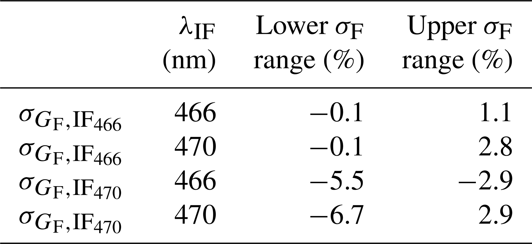
The values are summarized in Table 2. The lower and upper systematic relative biases correspond to the most negative and positive bias calculated from each spectrum of Fig. 1 (including both spectra from biomass burning aerosol and dust). This ensures that the error bars are conservative and cover the whole uncertainty range of the dataset displayed in Fig. 1. We see that IF_470,100 leads to generally larger biases, even at its central wavelength, with a tendency to underestimate the actual $G_{\mathrm{F}}^{\mathrm{355}}$ value. We further compare the biased $\stackrel{\mathrm{‾}}{G_{\mathrm{F},\mathrm{470}}^{\mathrm{355}}}$ and $\stackrel{\mathrm{‾}}{G_{\mathrm{F},\mathrm{466}}^{\mathrm{355}}}$ values which occur after transmission through IF₄₇₀ and IF₄₆₆, respectively. The relative difference between $\stackrel{\mathrm{‾}}{G_{\mathrm{F},\mathrm{470}}^{\mathrm{355}}}$ and $\stackrel{\mathrm{‾}}{G_{\mathrm{F},\mathrm{466}}^{\mathrm{355}}}$with respect to $\stackrel{\mathrm{‾}}{G_{\mathrm{F},\mathrm{466}}^{\mathrm{355}}}$ is defined as

$$\begin{array}{}\text{(10)}& {\mathit{\sigma }}_{\mathrm{\Delta }\mathrm{IF}}={\displaystyle \frac{\stackrel{\mathrm{‾}}{G_{\mathrm{F},\mathrm{470}}^{\mathrm{355}}}-\stackrel{\mathrm{‾}}{G_{\mathrm{F},\mathrm{466}}^{\mathrm{355}}}}{\stackrel{\mathrm{‾}}{\stackrel{\mathrm{‾}}{G_{\mathrm{F},\mathrm{466}}^{\mathrm{355}}}}}},\end{array}$$

and can range from −5.8 % to 0.6 % for the different spectra of Fig. 1.

Table 2 Relative systematic bias due to the IF transmission band. Values are calculated relative to the true spectral fluorescence capacities at 466 and 470 nm which have been taken from Reichardt et al. (2025).

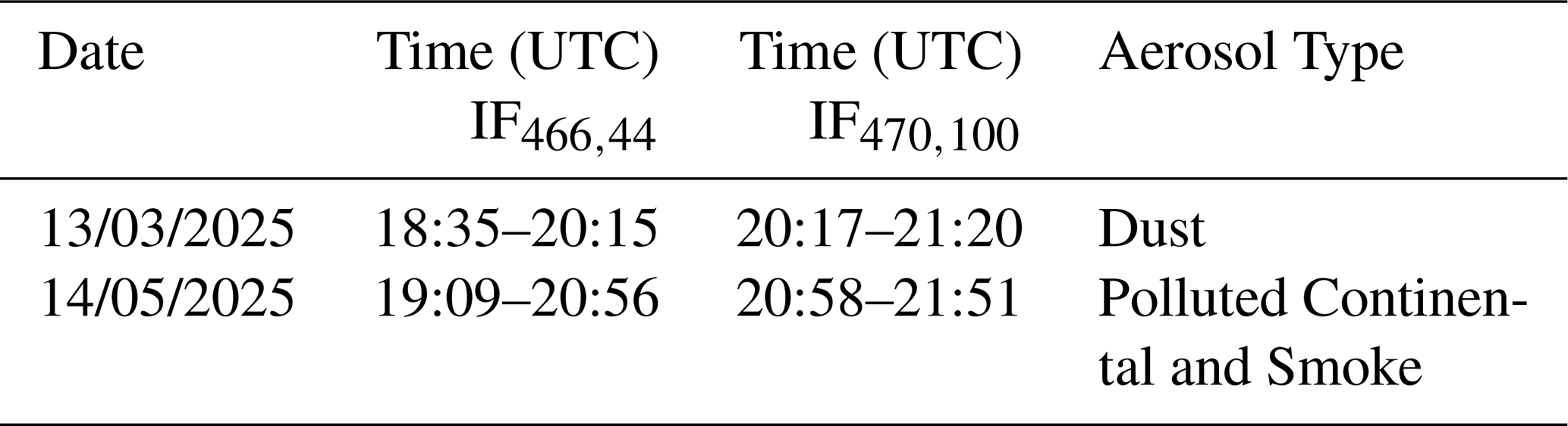
In order to compare the spectral fluorescence capacity considering the characteristics of IF_466,44 and IF_470,100 we use Eq. (7). The IF comparison test was performed on seven separate days in 2025. Here, we present two representative cases: one dominated by dust aerosols and another characterized by urban and smoke aerosols, used to compare the two IFs. Table 3 lists the dates and times of each measurement.

Table 3 Observation dates and UTC time windows for IF_466,44 and IF_470,100 fluorescence measurements.

Across the $G_{\mathrm{F}}^{\mathrm{355}}$, small differences are observed when comparing the IF_466,44 and the IF_470,100 over Thessaloniki (Fig. 2). For instance, on 13 March 2025, an extreme dust event passed over Thessaloniki, providing an opportunity to evaluate the performance of the two IFs (Fig. 2a). The aerosol layer extended from 0.65 to 3.2 km.

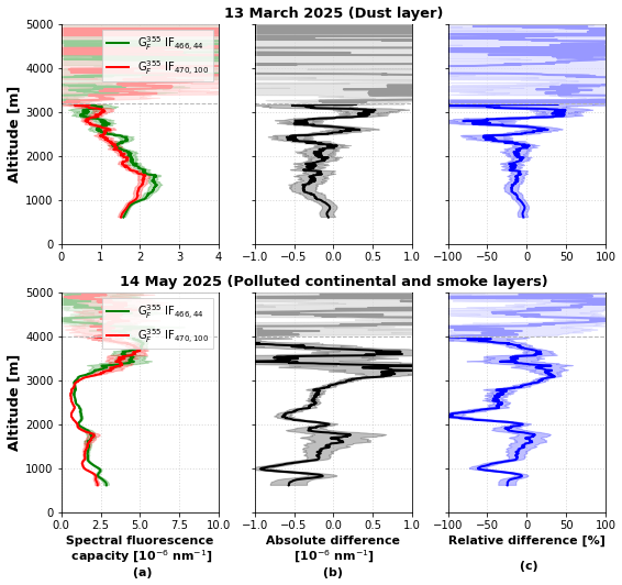
Figure 2 (a) Vertical profiles of mean $G_{\mathrm{F}}^{\mathrm{355}}$ for the two cases with subsequent measurements performed both with IF_466,44 (green) and with IF_470,100 (red) filters, (b) absolute difference and (c) relative difference expressed as percentage and normalized to $G_{\mathrm{F},\mathrm{470}}^{\mathrm{355}}$ on 13 March 2025 (dust layer) and 14 May 2025 (polluted continental and smoke layers). The uncertainties are propagated, assuming random errors using standard Gaussian error propagation.

Applying Eq. (7), we calculated $G_{\mathrm{F}}^{\mathrm{355}}$ using IF_466,44 and $G_{\mathrm{F}}^{\mathrm{355}}$ using IF_470,100, as shown in Table 4. These results indicate that the $G_{\mathrm{F}}^{\mathrm{355}}$ retrieved using the two different IFs is comparable and consistent with recent literature (Reichardt et al., 2025) and that Eq. (7) provides a useful approach for comparing $G_{\mathrm{F}}^{\mathrm{355}}$ values obtained between different lidar systems. As introduced by Reichardt et al. (2025), $G_{\mathrm{F}}^{\mathrm{355}}$ varies with aerosol type, therefore, a second case characterized by urban and smoke aerosols is presented in Fig. 2b and the calculated $G_{\mathrm{F}}^{\mathrm{355}}$ are again shown in Table 4.

Table 4 Spectral fluorescence capacity mean, minimum and maximum values using the IF_466,44 and the IF_470,100for the two dates.

Here, the observed differences between $G_{\mathrm{F},\mathrm{466}}^{\mathrm{355}}$ and $G_{\mathrm{F},\mathrm{470}}^{\mathrm{355}}$ (Fig. 2b, c) are much bigger than the systematic error estimation due to the IF transmission band especially for shallow layers, and also according to the error bars the noise is too low to explain the differences, which leads us to the conclusion that the variations were probably related to atmospheric changes between the two measurements as they were not performed simultaneously or iteratively.

These findings highlight the importance of standardizing spectral fluorescence capacity within EARLINET to enhance the comparability of fluorescence measurements and to improve aerosol characterization and typing schemes.

3 Observations and typing of fluorescence measurements

Fluorescence measurements have been performed since March 2024 in Thessaloniki. For all these measurements, geometrical properties (i.e., base, top, and center of mass) of the detected aerosol layers are analysed using the wavelet covariance transform (WCT) method in signal regions with sufficient signal-to-noise ratio. The WCT method allows the identification of multiple aerosol layers within a single profile, thus, providing insights into internal layer structure. The WCT method is applied in the aerosol backscatter coefficient profiles, preferably at 1064 nm since they exhibit stronger vertical gradients and clearer layer structures than extinction coefficient, particularly at longer wavelengths (Baars et al., 2008; Siomos et al., 2017). A key parameter in the analysis is the dilation parameter value, as it controls the sensitivity of the method to aerosol structures at different vertical scales. Larger dilation values highlight major aerosol layers, while smaller values allow the detection of finer structures. A dilation value of 0.3 km is applied in this study for the detection of lofted aerosol layers to be consistent with previous studies (e.g. Brooks, 2003; Baars et al., 2008).

For each distinct layer, identified by the WCT method, we calculated the mean value of the spectral fluorescence capacity, $G_{\mathrm{F}}^{\mathrm{355}}$, the particle linear depolarization ratio, PLDR₅₃₂, the backscatter related Ångström exponents, BAE${}_{\mathrm{355}/\mathrm{532}}$ and BAE${}_{\mathrm{355}/\mathrm{1064}}$, and the lidar ratios, LR₃₅₅ and LR₅₃₂. The type of each aerosol layer was classified using the EARLINET Mahalanobis distance-based typing algorithm (EMD), a method specifically developed for the use on the EARLINET database with a high level of flexibility in order to adapt to the different lidar setups and needs (Papagiannopoulos et al., 2018). The algorithm applies the Mahalanobis distance classifier (Mahalanobis, 2018) to classify observations into a maximum of eight (i.e., Dust (D), Volcanic (V), Mixed Dust (MD), Polluted Dust (PD), Clean Continental (CC), Mixed Marine (MM), Polluted Continental (PC), Smoke (S)) and a minimum of four (i.e., Dust, Maritime, Polluted Smoke, Clean Continental) aerosol classes, considering the needs of each user and the provided number of the intensive properties. EMD classification has previous been applied to the Thessaloniki EARLINET dataset during the period 2012–2015 to derive the predominant aerosol type (Voudouri et al., 2019). The intensive properties that held the most weight among others in the classification and are used in this analysis are the BAE${}_{\mathrm{355}/\mathrm{532}}$, LR₅₃₂, the ratio of the lidar ratios (LR${}_{\mathrm{532}}/{\mathrm{LR}}_{\mathrm{355}}$) and the PLDR₅₃₂.

In addition, to verify the origin of the detected aerosol layers, we calculated back trajectories by using the HYSPLIT model (Hybrid Single-Particle Lagrangian Integrated Trajectory; https://www.ready.noaa.gov/HYSPLIT.php, last access: 29 January 2026; Stein et al., 2015). Below, three case studies involving different types of aerosols and their properties are presented and analysed (Sect. 3.1–3.3). An aerosol classification approach based on spectral fluorescence capacity is applied to the full THELISYS dataset in Sect. 3.4.1. Finally, fluorescence-based aerosol typing and EMD classification approach are compared, identifying similarities and differences in the detected aerosol types and demonstrating the complementary nature of the two methods for aerosol characterization (Sect. 3.4.2).

3.1 Fluorescence properties of a smoke layer

During 2024 Canada experienced another severe wildfire season (Parrington and Tomaso, 2024). The wildfire activity began in April and persisted through June and July, with smoke plumes from these wildfires having undergone episodes of long-range transport across the Atlantic, reaching western, central and eastern Europe. THELISYS monitored the smoke layers throughout this period, and the case presented in Fig. 3 corresponds to a smoke transport event that persisted for 5 d (22–26 July 2024). The 5 d backward trajectories from HYSPLIT (Fig. 3f), calculated at the altitudes of the identified smoke layers (layers 3 and 4 in Table 5), in conjunction with fire locations from the MODIS FIRMS product (not shown here), confirm that the biomass-burning aerosol was transported from Canada to the region of Thessaloniki.

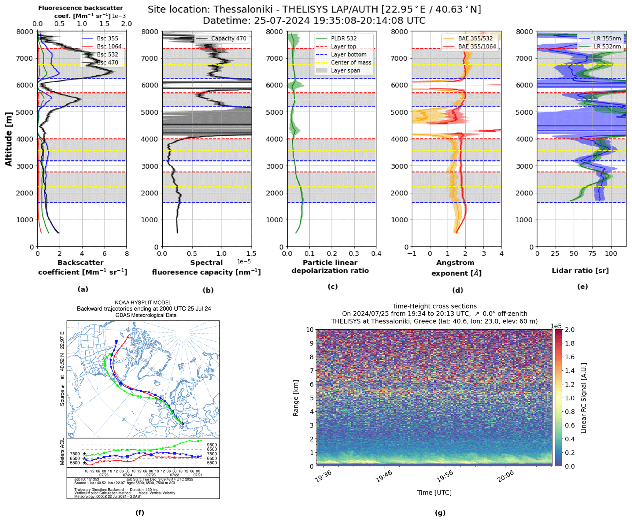
Figure 3 Vertical profiles of the backscatter coefficients (a), spectral fluorescence capacity (b), particle linear depolarization ratio (c), Angstrom exponents (d), lidar ratios (e), HYSPLIT backward trajectory model (f) and temporal evolution of the range corrected signal at 470 nm (g) on 25 July 2024.

Table 5 Mean values of the aerosol optical properties for the aerosol layers and aerosol type by EMD.

The retrieved profiles of the particle and fluorescence backscatter coefficients, spectral fluorescence capacity, particle depolarization ratio, lidar ratios and Angstrom exponents are presented in Fig. 3a–e. Four distinct layers of different aerosol types have been identified; the first two are below 4 km and the other two above 4.8 km.

The mean values for each layer are summarized in Table 5. Based on numerical values, as well as the corresponding vertical distribution, the two lowermost layers exhibit similar mean values of the aerosol optical properties, and their spectral fluorescence capacity remains below $\mathrm{2.5}\times {\mathrm{10}}^{-\mathrm{6}}$ nm⁻¹, indicating the presence of similar aerosols. Based on these characteristics, and supported by the EMD classification, both layers are identified as polluted continental. In the third layer, although the mean values of PLDR₅₃₂, BAE${}_{\mathrm{355}/\mathrm{532}}$, LR₃₅₅, and LR₅₃₂, together with the EMD, again point to a polluted continental aerosol type, the mean spectral fluorescence capacity $G_{\mathrm{F}}^{\mathrm{355}}$ value differs substantially, reaching $\mathrm{8.2}\times {\mathrm{10}}^{-\mathrm{6}}$ nm⁻¹ (fluorescence capacity, $G_{\mathrm{F}}=\mathrm{5.1}\times {\mathrm{10}}^{-\mathrm{4}}$). The increased $G_{\mathrm{F}}^{\mathrm{355}}$ value clearly indicates the presence of a different aerosol type in this layer, and, following the findings of Reichardt et al. (2025) for the spectral fluorescence capacity and of Gast et al. (2025) and Veselovskii et al. (2022b) for fluorescence capacity, we infer that this type corresponds to smoke. Finally, in the third layer, both the mean values of PLDR₅₃₂, BAE${}_{\mathrm{355}/\mathrm{532}}$, LR₃₅₅, LR₅₃₂ and the EMD, as well as the mean $G_{\mathrm{F}}^{\mathrm{355}}$ value, $\mathrm{9.0}\times {\mathrm{10}}^{-\mathrm{6}}$ nm⁻¹ ($G_{\mathrm{F}}=\mathrm{7.2}\times {\mathrm{10}}^{-\mathrm{4}}$), show that this layer corresponds to smoke.

3.2 Fluorescence properties of a dust layer

An extreme dust transport event was monitored by THELISYS in mid-March 2025, lasting 6 d (11–16 March 2025, Fig. 4). The 5 d backward trajectory analysis using HYSPLIT, combined with the DREAM8b-CAMS model (Basart et al., 2012, not shown), confirms that the detected dust plume originated from the Sahara and was transported to the Thessaloniki region (Fig. 4f).

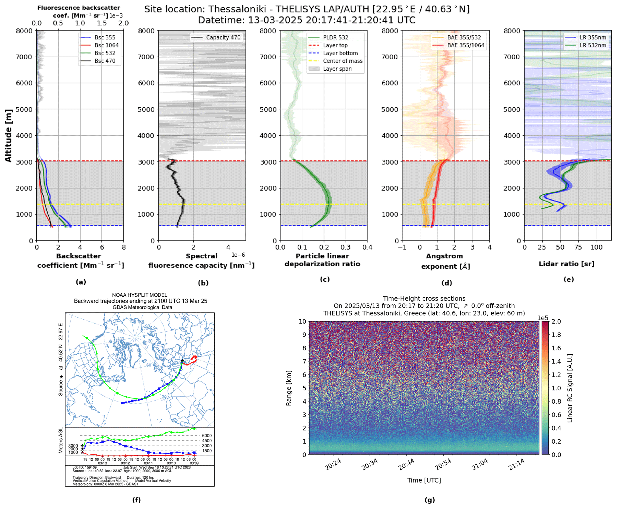
Figure 4 Vertical profiles of the backscatter coefficients (a), spectral fluorescence capacity (b), particle linear depolarization ratio (c), Angstrom exponents (d), lidar ratios (e), HYSPLIT backward trajectory model (f) and temporal resolution of the range corrected signal at 470 nm (g) on 13 March 2025. (Please note that for the spectral fluorescence capacity in panel (b) an x-axis scaling is employed which is different from the one used in the other figures.)

The retrieved profiles of the particle backscatter coefficients, spectral fluorescence capacity, particle depolarization ratio, lidar ratios and Angstrom exponents are shown in Fig. 4a–e. There is one aerosol layer recognized and the mean values for this layer are presented in Table 6. The retrieved optical properties values indicate the presence of coarse particles and are consistent with the typical mixed dust characteristics observed over Thessaloniki (Siomos et al., 2018; Voudouri et al., 2019). In addition, the mean spectral fluorescence capacity $\mathrm{0.92}\times {\mathrm{10}}^{-\mathrm{6}}$ nm⁻¹ ($G_{\mathrm{F}}=\mathrm{0.59}\times {\mathrm{10}}^{-\mathrm{4}}$) is quite low, in agreement with the findings of Reichardt et al. (2025) and Veselovskii et al. (2020) for the fluorescence capacity regarding the presence of mixed dust particles. The EMD likewise identifies this layer as mixed dust.

Table 6 Mean values of the aerosol optical properties for the dust layer and aerosol type by EMD.

3.3 Fluorescence properties of a mixed pollen layer

Komnos et al. (2022) findings showed that totally 10 pollen families and two fungi were recognized over Northwestern Greece. Damialis et al. (2007) reported that the taxa with the most abundant pollen atmospheric levels in Thessaloniki were those of Cupressaceae, Quercus, Urticaceae, Pinaceae, and Oleaceae; these comprised 72.5 % of the total pollen flora. A mixed pollen layer was detected by THELISYS on 20 February 2025 (Fig. 5). This observation coincides with the beginning of the pollen season in Greece, which generally lasts from February to September (Komnos et al., 2022; Damialis et al., 2007). The back-trajectory analysis demonstrates that the air masses in this episode were transported from the Balkans (Fig. 5f).

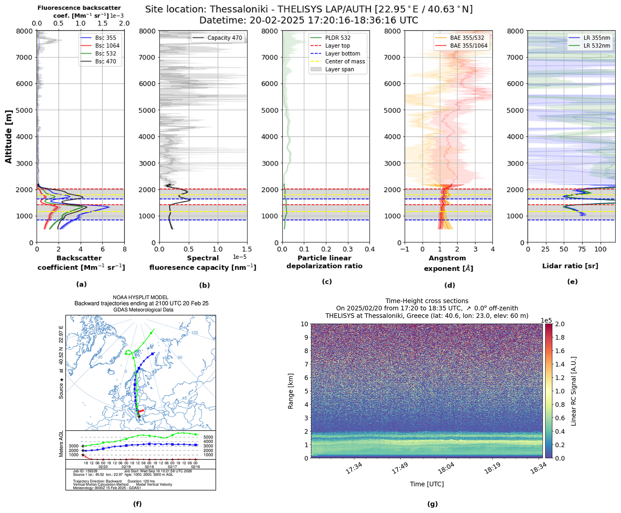
Figure 5 Vertical profiles of the backscatter coefficients (a), spectral fluorescence capacity (b), particle linear depolarization ratio (c), Angstrom exponents (d), lidar ratios (e), HYSPLIT backward trajectory model (f) and temporal resolution of the range corrected signal at 470 nm (g) on 20 February 2025.

The retrieved vertical profiles of particle backscatter coefficients, spectral fluorescence capacity, particle linear depolarization ratio, Ångström exponents and lidar ratio are shown in Fig. 5a–e. Two distinct aerosol layers are identified where the first layer extends from 0.8 to 1.4 km and the second from 1.6 to 2 km.

The mean values of the optical properties for each layer are shown in Table 7. In the first layer, the mean $G_{\mathrm{F}}^{\mathrm{355}}$ is only $\mathrm{1.8}\times {\mathrm{10}}^{-\mathrm{6}}$ nm⁻¹ ($G_{\mathrm{F}}=\mathrm{1.05}\times {\mathrm{10}}^{-\mathrm{4}})$, indicating the presence predominantly of polluted continental aerosols. The second layer exhibits a higher mean $G_{\mathrm{F}}^{\mathrm{355}}$ equal to $\mathrm{4.5}\times {\mathrm{10}}^{-\mathrm{6}}$ nm⁻¹ ($G_{\mathrm{F}}=\mathrm{2.3}\times {\mathrm{10}}^{-\mathrm{4}}$), a similar PLDR (0.02), and a higher BAE${}_{\mathrm{355}/\mathrm{532}}$ (1.22). The retrieved values in the second atmospheric layer, particularly the high fluorescence capacity observed at this altitude, together with the absence of confirmed biomass-burning aerosols on that day, suggest the presence of pollen. Veselovskii et al. (2021) reported fluorescence capacity values around $\mathrm{1.5}\times {\mathrm{10}}^{-\mathrm{4}}$ and particle linear depolarization ratio (PLDR) values at 532 nm around 0.1 for pollen, while Filioglou et al. (2023) found higher PLDR values under pollen-dominated conditions, approximately 0.28 for birch pollen and 0.43 for pine pollen when background aerosol contributions were minimal. In Thessaloniki, lower particle linear depolarization ratio values were retrieved, likely due to the mixing of pollen with urban aerosols and/or the presence of different pollen taxa. During the end of February, Alder and Cupressaceae pollen are present in the atmosphere (Komnos et al., 2022). Figure 6 presents the mean and accumulated Alnus (alder) pollen concentrations simulated by the CAMS ensemble median model over the broader Thessaloniki area for 19–20 February 2025. The figure also includes the daily Alnus pollen concentrations measured with a Hirst-type pollen trap in Thessaloniki during 2016–2022 (Charalampopoulos et al., 2021), providing historical context for the seasonal occurrence of alder pollen. Alnus pollen grains are approximately spherical, with diameters of 20–30 µm (Smith, 2000), and therefore fall within the coarse bioaerosol size range. Their presence could consequently have influenced the optical properties of the observed aerosol layer.

Table 7 Mean values of the aerosol optical properties for the aerosol layers and aerosol type by EMD.

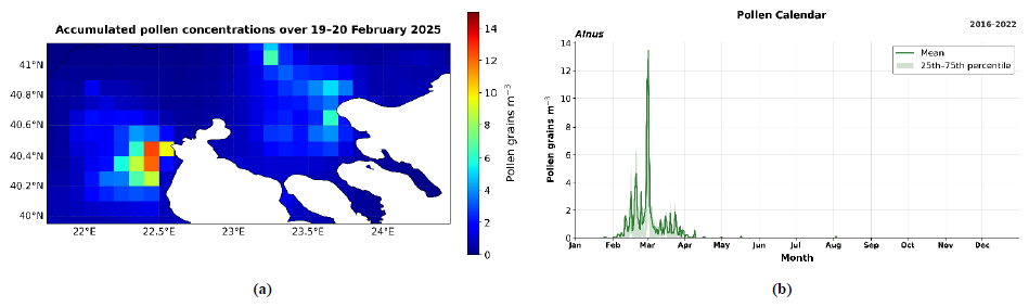
Figure 6 Accumulated Alnus pollen concentrations over the broader Thessaloniki area during 19–20 February 2025 (a) and pollen calendar of daily Alnus pollen concentrations (b). The solid green line represents the calendar-day mean, while the shaded area indicates the interquartile range (25th–75th percentiles).

3.4 Variability of aerosol types in Thessaloniki

3.4.1 Aerosol typing including spectral fluorescence capacity

The complete THELISYS dataset for the period between April 2024 and December 2025 is analysed as the cases above. From a total of 50 measurements, 108 layers are identified by the WCT method. All layers are located above the full-overlap region (i.e., 0.35 km), extending to altitudes exceeding 10 km, indicating the presence of both boundary-layer aerosols and elevated layers in the free troposphere.

Figure 7a illustrates the individual layers, with colours representing their corresponding $G_{\mathrm{F}}^{\mathrm{355}}$ values. The observed $G_{\mathrm{F}}^{\mathrm{355}}$ values span several orders of magnitude, from approximately 10⁻⁷ to 10⁻⁵. As shown, higher values ($G_{\mathrm{F}}^{\mathrm{355}}>\mathrm{3}\times {\mathrm{10}}^{-\mathrm{6}}$ nm⁻¹) are observed during the summer months at mid to high altitudes, particularly between 3 and 8 km, suggesting the presence of strongly fluorescent aerosols, commonly associated with biomass-burning smoke transported over long distances. Throughout the year, $G_{\mathrm{F}}^{\mathrm{355}}$ varies around $\mathrm{1}\times {\mathrm{10}}^{-\mathrm{6}}$ nm⁻¹ for aerosol layers residing mainly at low altitudes (<4 km), while lower values ($G_{\mathrm{F}}^{\mathrm{355}}<\mathrm{1}\times {\mathrm{10}}^{-\mathrm{6}}$ nm⁻¹) are observed for some specific dust events, totally clear days.

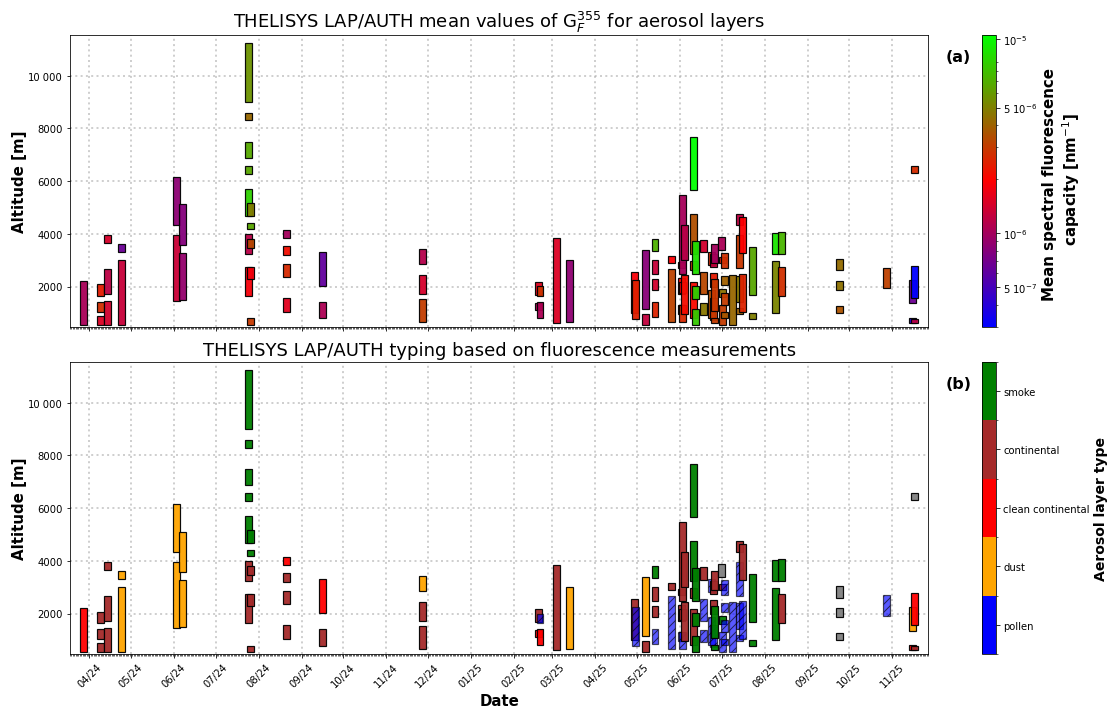
Figure 7 Vertical distribution of aerosol layers observed by THELISYS from April 2024 until December 2025. (a) Mean spectral fluorescence capacity $G_{\mathrm{F}}^{\mathrm{355}}$ for each detected aerosol layer, colours represent logarithmically scaled $G_{\mathrm{F}}^{\mathrm{355}}$ values. (b) Aerosol layer classification based mainly on spectral fluorescence capacity, with colours indicating the aerosol type. The vertical extent of each band denotes the base and top altitude of the detected layer. Blue hatched layers correspond to mixed pollen aerosol layers, for which the classification is considered less certain and remains under investigation compared to other aerosol types (the same applies to other figures).

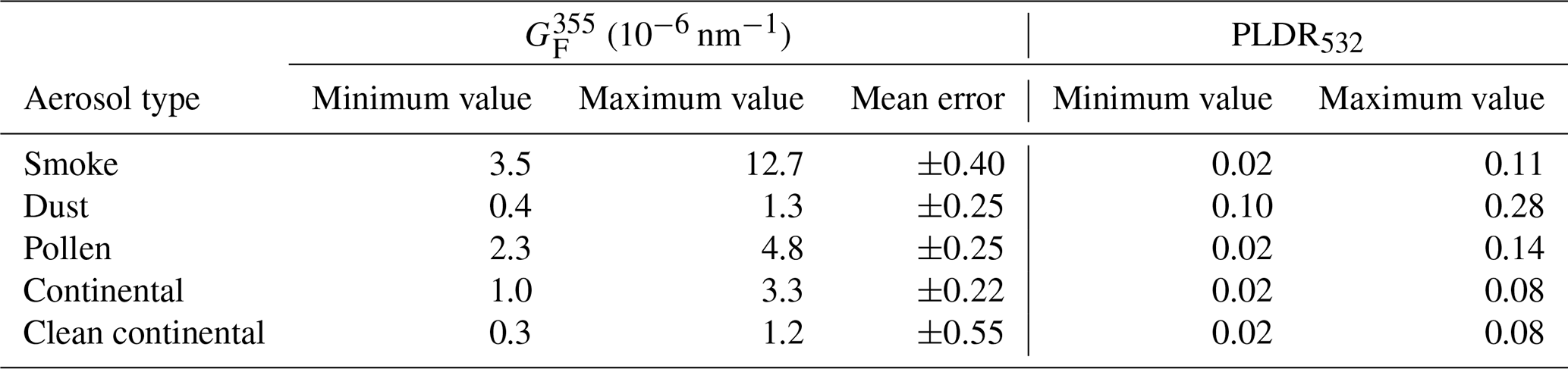
The classification of all layers was primarily based on the spectral fluorescence capacity and the particle depolarization ratio as shown in Table 8. For cases where the particle type was not clearly identified from these two parameters, the lidar ratio and backscatter Ångström exponent were also considered. In addition, the layer altitude was considered, since at different heights certain aerosols may exhibit similar spectral fluorescence capacity. For example, layers with biomass burning aerosols are typically observed above 4 km (Michailidis et al., 2024), whereas transported pollen layers are observed below 2.5 km (Damialis et al., 2017). Furthermore, the maximum layer value of the spectral fluorescence capacity was used to discriminate among clean continental ($\mathrm{0.6}\times {\mathrm{10}}^{-\mathrm{6}}$ nm${}^{-\mathrm{1}}<G_{\mathrm{F},max}^{\mathrm{355}}<\mathrm{1.8}\times {\mathrm{10}}^{-\mathrm{6}}$ nm⁻¹), polluted continental ($\mathrm{1.4}\times {\mathrm{10}}^{-\mathrm{6}}$ nm${}^{-\mathrm{1}}<G_{\mathrm{F},max}^{\mathrm{355}}<\mathrm{3.6}\times {\mathrm{10}}^{-\mathrm{6}}$ nm⁻¹) and mixed pollen ($\mathrm{2.3}\times {\mathrm{10}}^{-\mathrm{6}}$ nm${}^{-\mathrm{1}}<G_{\mathrm{F},max}^{\mathrm{355}}<\mathrm{6.4}\times {\mathrm{10}}^{-\mathrm{6}}$ nm⁻¹) aerosol. The presence of smoke and dust is further confirmed by the HYSPLIT trajectory model, other forecasting models, and satellite observations, as discussed in the two corresponding cases in Sect. 3.1 and 3.2. Table 8 summarizes the thresholds considered for the characterization of the different aerosol layers.

Table 8 Thresholds of fluorescence capacity, spectral fluorescence capacity, particle depolarization ratio and maximum spectral fluorescence capacity used for the characterization of the aerosol layers.

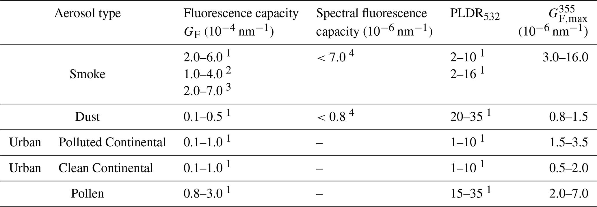
¹ Veselovskii et al. (2022b), ² Hu et al. (2022), ³ Gast et al. (2025), ⁴ Reichardt et al. (2025).

Based on the above criteria, Fig. 7b shows the classified aerosol types; smoke (green), dust (orange), continental (brown), clean continental (red), mixed pollen (blue). Overall, increased $G_{\mathrm{F}}^{\mathrm{355}}$ values are observed during the period from March to October, indicating enhanced concentrations of fluorescent aerosol components. This seasonal increase is attributed to the presence of aerosol mixtures influenced by both pollen emissions and biomass-burning aerosols. Especially, during the summer months (i.e., June–August), higher values in $G_{\mathrm{F}}^{\mathrm{355}}$ are evident, consistent with the frequent occurrence of smoke aerosols originating from regional wildfires in Greece or the Balkans as well as long-range transported biomass-burning plumes from North America (e.g., Canada), Russia, Eastern Europe (Amiridis et al., 2009). These smoke plumes are detected not only within the boundary layer but also at higher altitudes.

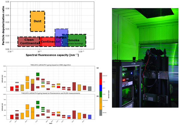
Based on the analysis of 50 cases of fluorescence lidar measurements obtained by THELISYS, Fig. 8 and Table 9, summarize the aerosol typing framework adopted in this study that relies on the combined use of spectral fluorescence capacity, with IF center wavelengths of either 466 or 470 nm, and the particle linear depolarization ratio at 532 nm. Dust particles, including mixed dust in this category, are characterized by low spectral fluorescence capacity and high depolarization ratios, which is consistent with their non-spherical mineral nature. Smoke aerosols exhibit significantly enhanced spectral fluorescence capacity combined with low depolarization values, reflecting the presence of biomass-burning particles at high altitudes during the summer months. Pollen particles exhibit a fairly high spectral fluorescence capacity with relatively low depolarization, supporting their identification primarily at lower to mid-tropospheric altitudes during the pollen season. It is important to note that their characterization is complicated by the fact that pollen particles frequently occur as part of mixed aerosol layers, often combined with urban, smoke or other aerosol types. Moreover, the particle linear depolarization ratio of pollen strongly depends on the dominant pollen taxa, which varies with geographic region and season, leading to additional variability in the observed optical properties. Continental aerosols show lower spectral fluorescence capacity and depolarization ratios compared to smoke and dust, indicating weaklier fluorescent and small particles, which are typically confined to the lower atmospheric layers.

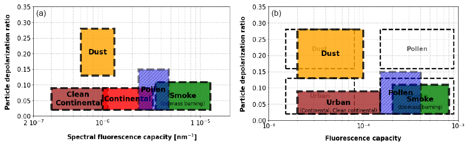
Figure 8 (a) Aerosol typing in Thessaloniki based on spectral fluorescence capacity and particle depolarization ratio and (b) based on fluorescence capacity and particle depolarization ratio. Empty dashed boxes adapted from Miri et al. (2025).

The results obtained from the analysed THELISYS measurement cases (colored boxes) show some differences from the values reported by Miri et al. (2025) (empty boxes) in Fig. 8b. For dust and smoke, consistent typing is observed, taking into account that the measurements were performed at different locations and during different periods. For urban aerosol, higher fluorescence capacity values are observed in the THELISYS measurements, indicating a contribution from fluorescent particles, that may be related to the influence of locally emitted smoke. More pronounced differences are observed for the mixed pollen layers, particularly in the particle depolarization ratio. As discussed in Sect. 3.3, these differences are likely related to the mixing of pollen with urban aerosols observed at the Thessaloniki lidar station or to differences in the dominant pollen taxa. Pollen grains from different taxa can exhibit different sizes, shapes, and morphological characteristics, which may consequently affect their optical properties, and particularly the particle depolarization ratio. It should also be noted that the proposed typing scheme may be influenced by particle hygroscopic growth, particularly under conditions of high relative humidity, as water uptake can modify particle size and consequently their optical properties, including the elastic backscatter coefficient and particle depolarization ratio (Miri et al., 2024).

Table 9 Characteristic ranges of layer mean spectral fluorescence capacity ($G_{\mathrm{F}}^{\mathrm{355}}$) and particle linear depolarization ratio (PLDR₅₃₂) for selected aerosol types.

3.4.2 Comparison of aerosol typing methods

The THELISYS lidar sub-dataset covering March 2024 to April 2025 was analysed for aerosol typing using both the EMD and the fluorescence capacity classification. For the 16 cases, 31 layers are identified by the WCT and all of them are above 350 m, as previously. EMD classified 29 layers (93 %), and 2 layers (7 %) were not assigned to any cluster showing an overall higher identification rate. Figure 9 presents the vertical distribution and temporal evolution of the aerosol layer types detected over Thessaloniki area. Across this period, layers are observed from near the surface up to approximately 8 km, indicating the presence of both boundary layer aerosols and elevated free-tropospheric layers. The dominant aerosol categories include dust and mixed/polluted dust (orange and dark orange), smoke (green), pollen (blue), clean continental (red), polluted continental (brown), and a small number of unclassified or unknown layers (grey), as inferred from the application of both EMD and fluorescence based aerosol typing.

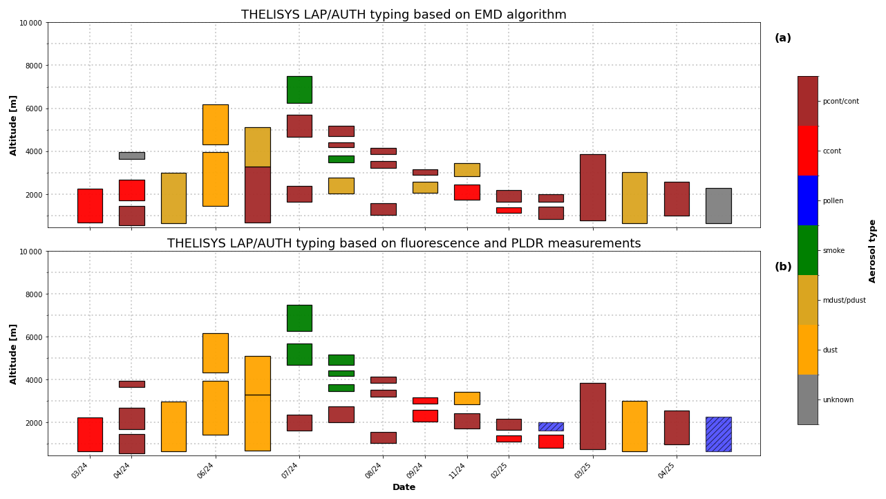
Figure 9 Vertical aerosol classification derived from (a) EMD, or (b) fluorescence properties.

From this dataset, it is evident that altitude layers below 2 km are dominated by clean and polluted continental aerosols, reflecting local and regional sources, while higher altitude layers are more frequently classified as dust, mixed dust, or smoke, indicating long-range transport processes. The highest altitude layers, occasionally extending beyond 8–9 km, are predominantly classified as polluted continental or smoke, especially in the EMD classification.

Figure 10 illustrates the overall differences in aerosol typing within the THELISYS dataset that emerge from the comparison of the two classification approaches. We considered the EMD output as the reference in our study because EMD has previously been applied in EARLINET dataset and been validated as a reliable method for typing (Voudouri et al., 2019; Mylonaki et al., 2021). Thus, each row is normalized by the total number of components identified by the EMD algorithm. Dust and mixed-dust layers (summarized as dust in Fig. 10) are consistently detected by both methods (75 % agreement), as the particle depolarization ratio plays a critical role in the separation of dust aerosols. A similarly high agreement is observed for smoke aerosols, with all EMD classified smoke layers assigned to the smoke fluorescence category. However, the number of smoke cases in the dataset is limited. For polluted continental aerosols, a partial agreement (53.3 %) is found between the two methods. The EMD classification overlaps with multiple fluorescence categories (e.g. smoke 20 %) suggesting that the spectral fluorescence capacity is a very useful parameter especially for the separation between smoke and polluted continental aerosols, as smoke is a highly fluorescing aerosol compared to others. Clean continental aerosols exhibit a lower agreement (50 %), with difficulty in separation of polluted and clean continental aerosols. This separation based on their fluorescence capacity values is at an initial stage of analysis and remains under investigation. The same applies to pollen detection. In the present dataset, only two mixed pollen layers were identified based on high fluorescence capacity values. Of these, one was classified as polluted continental by the EMD method, while the other remained unclassified. Mixed pollen layers are also under investigation and represent a promising opportunity for further development of aerosol typing algorithms.

Figure 10 Confusion matrix between EMD (truth) and fluorescence aerosol typing (prediction).

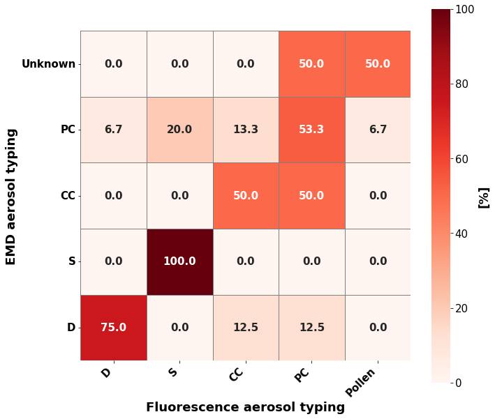
We conclude that aerosol typing using fluorescence channel capabilities, in combination with existing aerosol properties (e.g., particle depolarization ratio, Ångström exponent, and lidar ratio), could help in clearer separation between dust, smoke and mixed pollen layers. Overall, the comparison makes their combined use valuable for a more accurate characterization of aerosol vertical structure and source attribution.

4 Conclusion

In this study, fluorescence lidar observations from the upgraded THELISYS system were used to investigate aerosol typing over Thessaloniki, an urban site strongly influenced by a wide range of natural and anthropogenic aerosol sources. The detected aerosol layers were classified, for the first time, using both the spectral fluorescence capacity and the particle depolarization ratio, and were further intercompared with a conventional lidar derived optical properties classification scheme, developed within EARLINET.

Case studies of long-range transported biomass-burning smoke, Saharan dust intrusions, and mixed pollen layers highlighted the added value of fluorescence measurements in discriminating between these and polluted continental aerosols. Dust layers consistently exhibited low spectral fluorescence capacity and high depolarization ratios, while mixed pollen layers showed enhanced spectral fluorescence capacity at lower altitudes ($>\mathrm{2}\times {\mathrm{10}}^{-\mathrm{6}}$ nm⁻¹), reflecting the biological origin of the particles. These results confirm that spectral fluorescence capacity could provide complementary information for aerosol typing.

The analysis of a larger THELISYS dataset spanning more than one year of measurements revealed clear seasonal and vertical patterns in spectral fluorescence capacity. High values (greater than $\mathrm{3.6}\times {\mathrm{10}}^{-\mathrm{6}}$ nm⁻¹) were predominantly observed during the summer months and at elevated altitudes, associated with biomass-burning smoke, whereas values around unity occurred throughout the year, mainly within the boundary layer. Low spectral fluorescence capacity ($<\mathrm{1}\times {\mathrm{10}}^{-\mathrm{6}}$ nm⁻¹) values were linked to dust events.

Overall, this work demonstrates that the integration of fluorescence measurements into operational Raman lidar systems significantly improves the aerosol classification, particularly in complex environments such as the Eastern Mediterranean. The results support the future inclusion of spectral fluorescence capacity as a standard intensive parameter within EARLINET and ACTRIS frameworks and underline the need for harmonized fluorescence retrievals across the different lidar configurations. Future work will focus on expanding the statistical basis of the dataset, refining mixed-aerosol classification, and exploiting spectral fluorescence information to further enhance aerosol source attribution.