Characterizing variability and vertical structure of water vapor in the extratropical lower stratosphere

Stratospheric water vapor strongly affects Earth’s radiative balance, especially in the extratropical lower stratosphere, yet large uncertainties remain regarding its variability, long-term trends and relationships to tropopause behavior. Here we characterize the seasonality, vertical structure, and variability of water vapor near the extratropical tropopause and the extratropical transition layer (ExTL). We analyze 17 years (2005–2021) of satellite observations from the Aura Microwave Limb Sounder (MLS) and the Atmospheric Chemistry Experiment Fourier transform spectrometer (ACE-FTS), with simulations from the Whole Atmosphere Community Climate Model (WACCM) using specified dynamics calculations. Analyses are performed in geometric and tropopause-relative vertical coordinates to assess the influence of coordinate on variability. Tropopause-relative coordinates substantially reduce variance in ExTL water vapor, but artificially enhance variability in the tropical upper troposphere. Tropopause-relative coordinates reveal a clear distinction between variability in the ExTL and the stratospheric overworld approximately 2.5 km above the tropopause. Above this level, there are hemispherically coherent anomalies linked to transport of air originating in the tropics. In contrast, ExTL variability lacks hemispheric coherence and likely reflects smaller-scale stratosphere-troposphere exchange. Interannual changes in ExTL water vapor show a statistically significant negative trend in both hemispheres in MLS data, but that behavior is not reproduced in ACE-FTS measurements or WACCM simulation. Despite this, the datasets agree well on overworld variability and regression responses to climate oscillations. The uncertainty in ExTL trends highlights the need for continued evaluation of long-term satellite records and improved model representation in this climatically sensitive layer.

1 Introduction

Stratospheric water vapor (H₂O) is a critical component of Earth’s radiative budget, and despite extremely low values relative to the troposphere even small changes in its concentration can have outsized impacts on surface temperatures and stratospheric circulation (Charlesworth et al., 2023; Solomon et al., 2010; Forster and Shine, 2002). H₂O in the extratropical lower stratosphere is especially important for radiative feedbacks (Charlesworth et al., 2023; Li and Newman, 2020; Banerjee et al., 2019; Dessler et al., 2013), although the magnitude of such a feedback is still debated and results can depend on the models and method used in the calculation (He and Huang, 2025). The tropopause in the extratropics is a complex transition region between the troposphere and stratosphere, with strong gradients in H₂O, ozone, and other constituents and an interplay of large- and small-scale circulations and radiative processes; this transition region is often referred to as the Extratropical Transition Layer (ExTL; e.g., Gettelman et al., 2011).

When studying stratospheric H₂O it can be useful to separate the stratosphere into different regions due to the underlying controlling processes and modes of transport. Specifically, the stratosphere is frequently divided into the stratospheric overworld and the (extratropical) lowermost stratosphere. The stratospheric overworld is conventionally defined as the region of the stratosphere above the 380 K isosurface of potential temperature, where composition is controlled by a source region near the tropical tropopause and the stratospheric transport circulation (Stohl et al., 2003; Holton et al., 1995; Hoskins, 1991). The lowermost stratosphere (LMS; also called the “middleworld”) is the region in the extratropics that exists below the 380 K isentrope but above the extratropical tropopause. Isentropes in the extratropical LMS cross into the tropical upper troposphere, but the subtropical jet acts as an effective transport barrier between these regions (Haynes et al., 2001). Overworld H₂O is controlled by two main processes: upward transport through the tropical tropopause via the Brewer-Dobson Circulation (BDC; e.g., Butchart, 2014) and methane oxidation in the upper stratosphere (e.g., Tao et al., 2023; Yu et al., 2022; le Texier et al., 1988). Air is freeze dried as it ascends into the stratosphere and the temperature of the tropical tropopause controls H₂O concentrations. Randel and Park (2019) demonstrated that tropical cold point temperatures (CPT) explain more than ∼80 % of the variability in global stratospheric overworld H₂O concentrations. Variations in CPT then leave a vertically and horizontally propagating imprint on overworld stratospheric H₂O, commonly referred to as the “atmospheric tape recorder” (Mote et al., 1996). In contrast, transport in the LMS is more complex, where stratosphere-troposphere exchange can be facilitated by Rossby wave breaking events, tropospheric intrusions, midlatitude cyclones, and tropopause-overshooting convection (e.g., Chang et al., 2023; Tinney and Homeyer, 2021; Homeyer and Bowman, 2013; Homeyer et al., 2011; Pan et al., 2009; Olsen et al., 2008). These processes complicate H₂O variability in the LMS, and their relative contributions are not well understood. A further complicating factor is the large variation in the tropopause structure itself on timescales of days to decades, including a large seasonal cycle in midlatitudes. Global observations of stratospheric water vapor are primarily collected by satellites with relatively low horizontal and vertical resolution, further limiting study of this region. Another complication is that global circulation models routinely overestimate the amount of LMS H₂O in historical and present climates (e.g., Charlesworth et al., 2023), contributing to poor understanding of this region.

The objective of this work is to analyze the seasonal and interannual variability and vertical structure of stratospheric H₂O in the LMS and across the ExTL using satellite observations and a global chemistry-climate model. Specifically, we use a 17-year period of observations from the Aura Microwave Limb Sounder (MLS) and SCISAT-1’s Atmospheric Chemistry Experiment Fourier transform spectrometer (ACE-FTS) in conjunction with simulations using the Whole Atmosphere Community Climate Model (WACCM) run in specified dynamics mode with observed meteorological fields. We aim to quantify variability and highlight the role of different sources in shaping the distribution of H₂O throughout the LMS. A key aspect of this work includes analysis in tropopause-following coordinates, in addition to standard geometric coordinates.

2 Data and Methods

2.1 MLS

Measurements of water vapor, ozone, and temperature from 2005–2021 are sourced from the Earth Observing System (EOS) MLS aboard the Aura satellite, version 5.0x. While MLS data continue to 2026, our analyses use data to 2021 to avoid impacts of the Hunga Tonga-Hunga Ha'apai eruption in early 2022 (Millán et al., 2022). Aura was launched in 2004 into a sun-synchronous satellite orbit with Equator crossing times of 01:30 and 13:30 local time as part of the NASA A-Train satellite constellation. MLS measures ∼3600 profiles per day with a 1.5° along-track separation between measurements (Livesey et al., 2022). The retrieval range of MLS measurements varies by species; water vapor is observed from 316–0.001 hPa, ozone from 261–0.001 hPa and temperature from 261–0.00046 hPa, and the data are quality-controlled following the recommendations of Livesey et al. (2022). Retrievals are provided on a regular pressure grid, with data at 12 levels per decade of pressure (∼1.25 km vertical sampling) for pressures greater than 1 hPa. The precision, accuracy, horizontal resolution, and vertical resolution of each species vary by altitude and are described in detail in Livesey et al. (2022). In our region of focus in the UTLS, the effective vertical resolution is ∼3 km for water vapor and ozone. The data analyzed here are monthly, zonal averages of level 2 (orbital) data binned in 2° latitude bins, which contain on the order of 1000 measurements per month over midlatitudes.

We note that the previous version 4.x MLS data exhibited a spurious positive H₂O drift in the stratosphere that was identified by Hurst et al. (2016). Livesey et al. (2021) further identified that there was an increasing drift associated with the 190 GHz sideband fraction in the MLS measurement, and this was subsequently addressed and partially ameliorated in version 5.x processing. However, the MLS instrument team suggests continued caution in studies evaluating H₂O trends using version 5 data (Livesey et al., 2022, 2021).

2.2 ACE-FTS

We also analyze satellite water vapor observations from the ACE-FTS (hereafter ACE) instrument from 2005–2021, using the version 5.2 retrieval (Bernath et al., 2005). ACE measures solar occultation spectra between 750 and 4400 cm⁻¹ at a spectral resolution of 0.02 cm⁻¹ to retrieve vertical profiles of temperature, pressure, and trace gas volume mixing ratios from the cloud tops to approximately 150 km. Altitude is the native vertical coordinate for these retrievals and the effective vertical resolution in the UTLS is about 3 km, oversampled at 1 km spacing. The instrument typically measures 30 profiles per day, requiring a three-month period to achieve near-global coverage (85° N–85° S). H₂O validation of the ACE-FTS instrument in the UTLS is discussed in depth by Hegglin et al. (2009). The recommended ACE v5.2 quality-control flags described in Sheese et al. (2015) are applied to remove scientifically unsuitable profiles prior to analysis. We perform an additional simple quality control measure to eliminate extreme and non-physical measurements (particularly near and below the tropopause) from the dataset by removing data points that fall outside of the 2nd and 98th percentile values for their specific height and latitudinal region. Because of the much sparser sampling of ACE compared to MLS, we use 3-month (DJF, MAM, etc.) averages in 10° latitude bins, which typically contain ∼20–100 measurements over midlatitudes. We require a minimum of 10 data points per 3-month 10° latitude bin for a valid data sample. Because of frequent loss of ACE-FTS retrievals below the tropopause (due to clouds or other problems) there are often missing data, and these regions are indicated as data voids in the figures below.

2.3 WACCM

Numerical experiments were conducted using the Community Earth System Model version 2 with the Whole Atmosphere Community Climate Model version 6 as its atmospheric component (CESM2/WACCM6; Danabasoglu et al., 2020; Gettelman et al., 2019). WACCM6 is a state-of-the-art chemistry–climate model that extends from the Earth’s surface to approximately 140 km and includes comprehensive troposphere–stratosphere–mesosphere–lower thermosphere (TSMLT) chemistry. In this study, WACCM6 is run in a specified-dynamics configuration (WACCM6-SD), with prescribed sea surface temperatures and sea ice. The simulations provide daily data covering the period 1980–2022 and use a horizontal resolution of 0.9° latitude ×1.25° longitude with the finite-volume dynamical core (Lin and Rood, 1996). The model includes 70 vertical levels from the surface to ∼140 km, with a vertical resolution of approximately 500 m in the upper troposphere and lower stratosphere (UTLS). In the specified-dynamics configuration, temperature and winds (U, V) are nudged toward the Modern-Era Retrospective Analysis for Research and Applications Version 2 (MERRA-2) reanalysis (Gelaro et al., 2017) using a 12 h relaxation timescale. This configuration has been shown to realistically reproduce key modes of stratosphere–troposphere coupling, including the quasi-biennial oscillation and stratospheric sudden warmings. It also provides a realistic representation of large-scale transport in the UTLS region and has been widely used in troposphere–stratosphere transport studies (e.g., Zhang et al., 2025; Pan et al., 2022; von Hobe et al., 2021). For a direct comparison with MLS, we restrict the analysis to 2005–2021, interpolate to the MLS vertical grid, and compute monthly, zonal averages in 2° latitude bins.

2.4 Tropopause-relative coordinates

Studies of UTLS composition can benefit from analyses using alternative coordinate systems, both vertically and horizontally (Millán et al., 2024). Various vertical coordinate systems can be used to reduce the composition variability associated with changes in tropopause height to isolate other sources of variability, such as from stratosphere-troposphere exchange. For analysis of H₂O in the lowermost stratosphere, tropopause-relative altitude is a common vertical coordinate and has been frequently used in previous studies (e.g., Tinney and Homeyer, 2021; Bland et al., 2021; Schwartz et al., 2015; Gettelman et al., 2011; Tilmes et al., 2010; Pan et al., 2004).

In this study we conduct analyses in both geometric (e.g. pressure, altitude) and tropopause-relative coordinates. Tropopause-relative calculations are computed for daily observations before aggregating the results into monthly (MLS, WACCM) or 3-monthly (ACE) means. For ACE and MLS, a reference tropopause is computed from three-hourly MERRA-2 reanalysis data (Gelaro et al., 2017) and interpolated in space and time to each profile location. The tropopause is also calculated daily in WACCM6 as the reference for the model profiles. Since the model is nudged to MERRA-2, these two tropopause datasets are nearly identical. The results shown here use the potential temperature gradient tropopause (PTGT; Tinney et al., 2022) as the reference tropopause definition. We also tested tropopause-relative calculations using the World Meteorological Organization (WMO; World Meteorological Organization, 1957) lapse-rate tropopause definition, finding consistent results with the PTGT (not shown). For MLS and WACCM, data is placed into tropopause-relative logarithmic pressure bins with a resolution corresponding to 12 levels per decade of pressure (Δz∼1.25 km), while ACE observations are placed into 1 km tropopause-relative altitude bins. Monthly zonal means are then computed for MLS and WACCM data and three-monthly seasonal means are computed for ACE. The tropopause-relative vertical coordinates are transformed back into an estimated geometric coordinate using the climatological mean tropopause pressure, with the logarithmic pressure bins becoming a “pseudo-pressure” coordinate. Some of our results include (area-weighted) extratropical tropopause averages, including monthly/seasonal data points poleward of 20° N/S where the local tropopause pressure exceeds 150 hPa, indicative of the lower-tropopause (extratropical) environments poleward of the tropopause break (Boothe and Homeyer, 2017; Homeyer and Bowman, 2013; Randel et al., 2007). This requirement constrains the analysis to at least partially exclude summer monsoon anticyclones, which frequently exhibit tropopause pressures of <150 hPa (Liu et al., 2014).

An example of the H₂O variability compared in geometric vs. tropopause-relative coordinates is illustrated in Fig. 1a–b, showing time series of MLS, ACE, and WACCM data at one location near the midlatitude tropopause (45° N, 215 hPa, 12 km). In geometric coordinates (Fig. 1a) there is a large annual cycle of H₂O with maxima during boreal summer, which closely follows the well-known annual cycle in midlatitude tropopause pressure (Fig. 1c). Time series in tropopause-relative coordinates (Fig. 1b) show a much smaller annual cycle, with smaller maxima during boreal summer. The comparisons in Fig. 1a–b show larger H₂O values near the extratropical tropopause for WACCM compared to MLS and ACE, and this is a general behavior as shown and discussed further below.

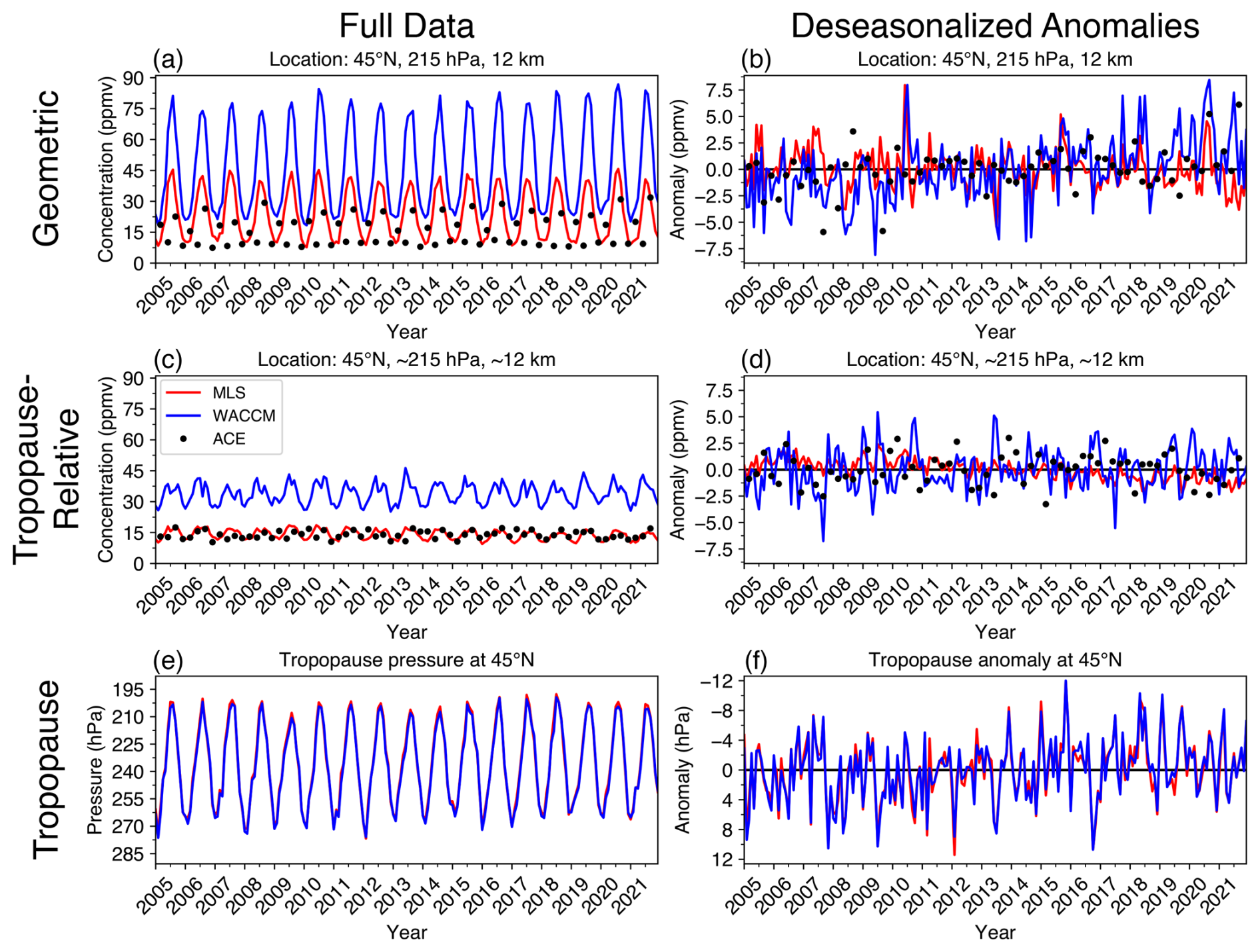
Figure 1 Upper and middle panels show time series of zonal mean H₂O at 45° N, 215 hPa (12 km), close to the midlatitude tropopause, from MLS data (red), ACE data (black dots), and WACCM simulation (green). (a) time series in geometric coordinates, (b) time series in tropopause-relative coordinates. Variations in tropopause pressure are shown in (c). Panels (d)–(f) show the corresponding deseasonalized anomalies.

Time series of the respective deseasonalized anomalies are shown in Fig. 1d–f. Tropopause-relative calculations (Fig. 1e) show a reduction in H₂O variance around the midlatitude tropopause compared to geometric coordinates by ∼30 % (Fig. 1d), due to removal of variability tied to the dynamic tropopause. This reduction in variance is consistent with the results of Hegglin et al. (2009). Figure 2 shows global comparisons of deseasonalized H₂O variance in the two coordinate systems. In geometric coordinates (Fig. 2a) there are maxima concentrated around the ExTL region of both hemispheres concentrated in the ExTL region, primarily linked with variations in the tropopause itself. Calculations in tropopause-relative coordinates (Fig. 2b) substantially reduce the ExTL variability, as the variance associated with changes in the height of the tropopause is removed. Similar patterns are found when this analysis is conducted on the WACCM simulation (not shown).

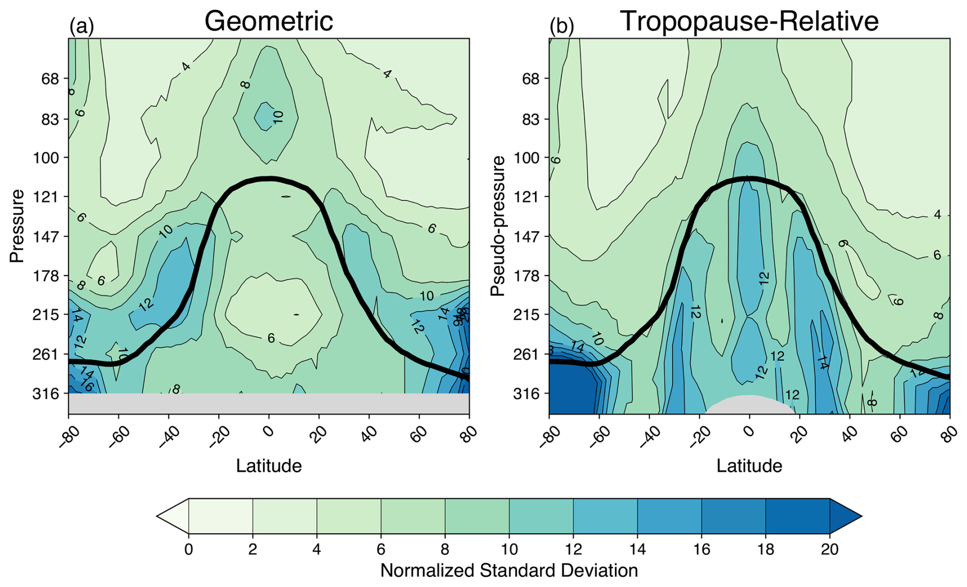
Figure 2 The normalized standard deviation for deseasonalized MLS H₂O anomalies in (a) geometric and (b) tropopause-relative coordinates. Values are in % compared to the time average background H₂O. The average height of the PTGT is shown as the solid black line.

In contrast to the reduction of variance near the ExTL, the use of tropopause-relative coordinates substantially increases H₂O variability throughout the tropical upper troposphere and below the subtropical jets (Fig. 2b – note maxima near 30° N and S and near the equator). This is an artifact of the tropopause-relative coordinate calculations. The tropical upper troposphere is characterized by strong vertical gradients in water vapor concentration, and small variations in tropopause altitude can lead to large changes in tropopause-relative water vapor. We find that much of the enhanced H₂O variance in this region is due to low frequency changes in tropopause height driven by ENSO and QBO variations (Randel et al., 2000). As a result, using tropopause-relative coordinates introduces artificial H₂O variability in the tropical upper troposphere, and is a poor coordinate choice for this region. Similarly, the increased variance in Antarctic tropopause-relative tropospheric H₂O stems from strong variations in the identified tropopause, where extreme stability makes tropopause identifications difficult. While the PTGT used here improves upon the frequent tropopause misidentifications by the LRT in polar winter, there are likely still cases where the diagnosed tropopause artificially increases the H₂O variability in the polar upper troposphere. However, this has minimal impact on our results focused on the extratropics.

3 Results

3.1 Time mean structure

Long-term average (2005–2021) cross sections of H₂O from MLS, ACE and WACCM are shown in Fig. 3, with results in both geometric and tropopause-relative coordinates. Patterns highlight the moist troposphere, dry stratosphere and strong gradients across the global tropopause. The tropopause-relative calculations highlight local vertical stratification in the extratropics compared to “fuzzy” structure in geometric coordinates. Careful comparison of the WACCM vs. MLS (or ACE) observations shows enhanced WACCM moisture in the extratropical lowermost stratosphere, and this is quantified in the (WACCM-MLS)/MLS percentage differences shown in Fig. 4. Compared with MLS, WACCM H₂O is more than 300 % higher in polar regions and more than 200 % higher in subtropical environments in the lower stratosphere of both hemispheres. Such moist biases in the LMS are a common problem for global models, as highlighted in Charlesworth et al. (2023). We note that this biased H₂O behavior is not simply due to circulation or temperature biases in WACCM, as our simulations use specified dynamics calculations with observed meteorological fields.

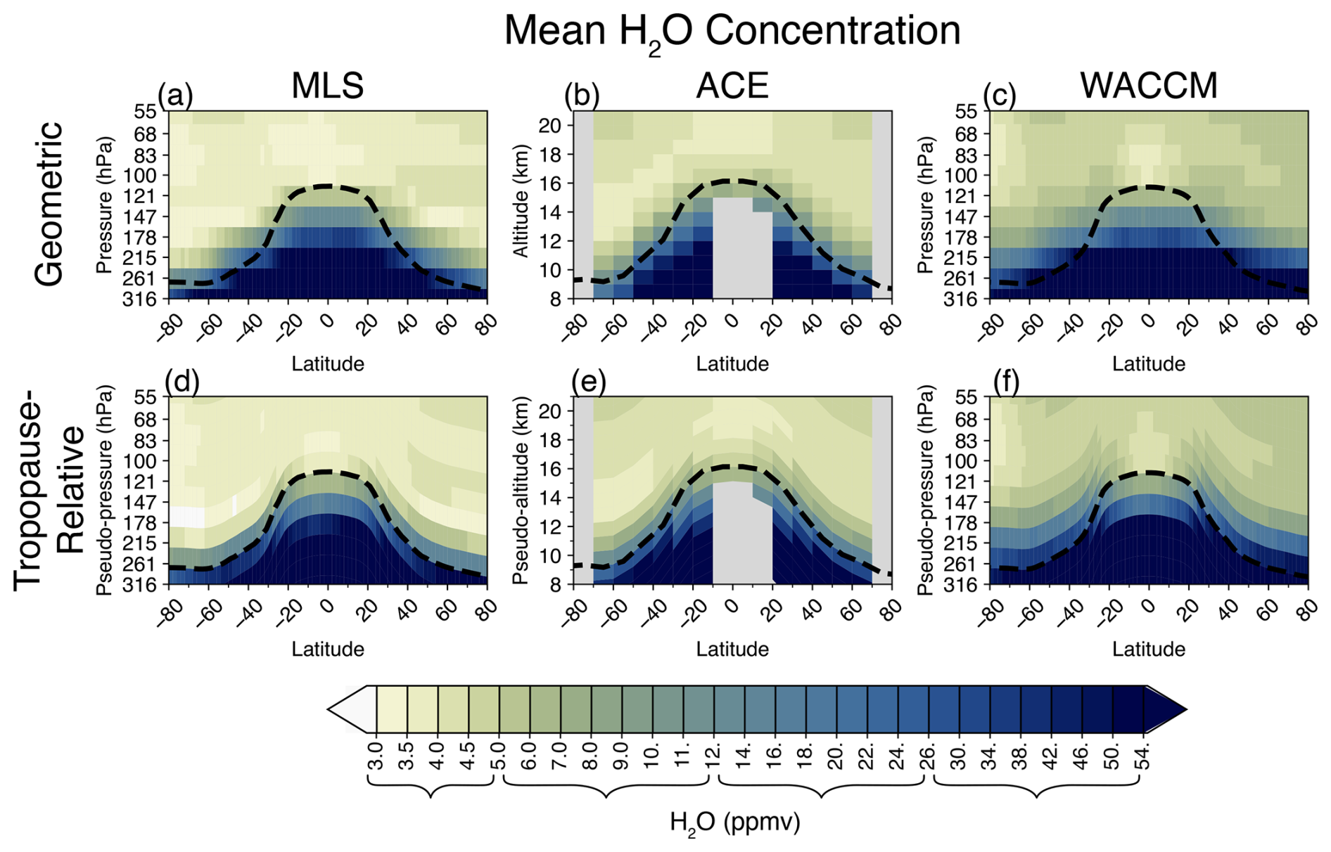
Figure 3 Time average H₂O from MLS, ACE and WACCM (left to right), analyzed in geometric (a–c) and tropopause-relative coordinates (d–f). ACE data is masked in gray where sampling is limited (<10 observations across 17 years.) Curly brackets on the color bar delineate grouped value ranges corresponding to a non-uniformly spaced discrete scale.

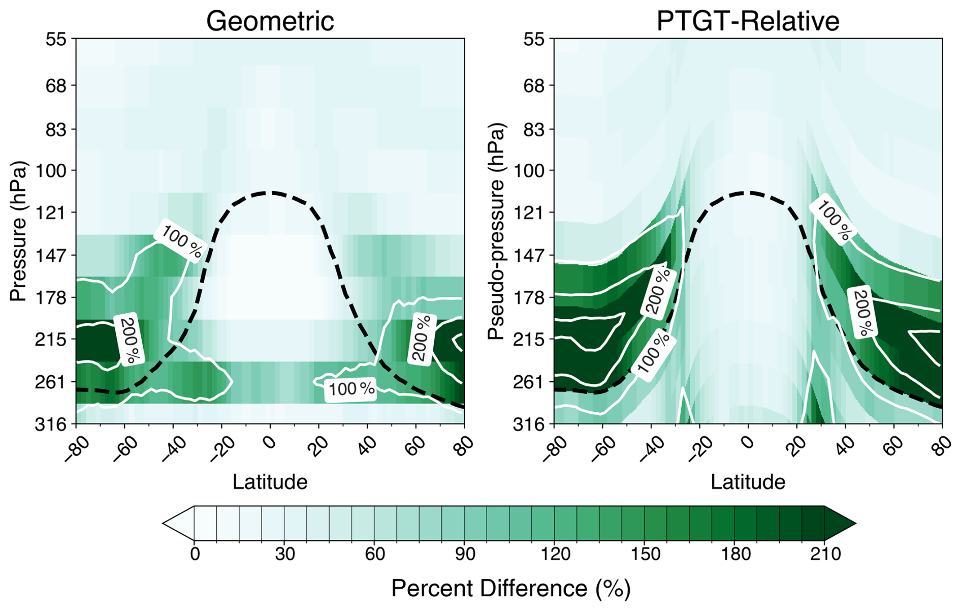
Figure 4 Time average H₂O differences between WACCM and MLS. Results are calculated as percentage (WACCM-MLS)/MLS values.

3.2 Seasonal ExTL behavior

Seasonal averages in zonal mean tropopause-relative H₂O concentration and atmospheric temperature as observed by MLS are shown in Fig. 5. The tropopause acts as a transport barrier in the extratropics, where there is a sharp gradient in all seasons and in both hemispheres. In the deep tropics, tropopause temperatures vary from ∼192 K in December, January, and February (DJF) to more than 196 K in June, July, and August (JJA). This seasonal pattern is reflected by in-phase H₂O concentrations at the tropical tropopause (low H₂O during DJF), and this seasonal minimum subsequently propagates upwards in the tropics and spreads in latitude in the lower stratosphere over most of the globe, demonstrating the well-known “tape recorder” signal (Mote et al., 1996). The meridional transport of air via the shallow branch of the BDC is evident in the dry layers extending along isentropic layers to higher latitudes in MAM and all the way to the North Pole in JJA. Notably, this seasonally-varying dry layer does not extend all the way down to the tropopause in the extratropics but stays above ∼215 hPa in the pseudo-pressure coordinates. Air in between this dry layer and the extratropical tropopause is wetter and is a signature of the ExTL. The summer hemisphere ExTL is particularly enhanced relative to the background stratosphere.

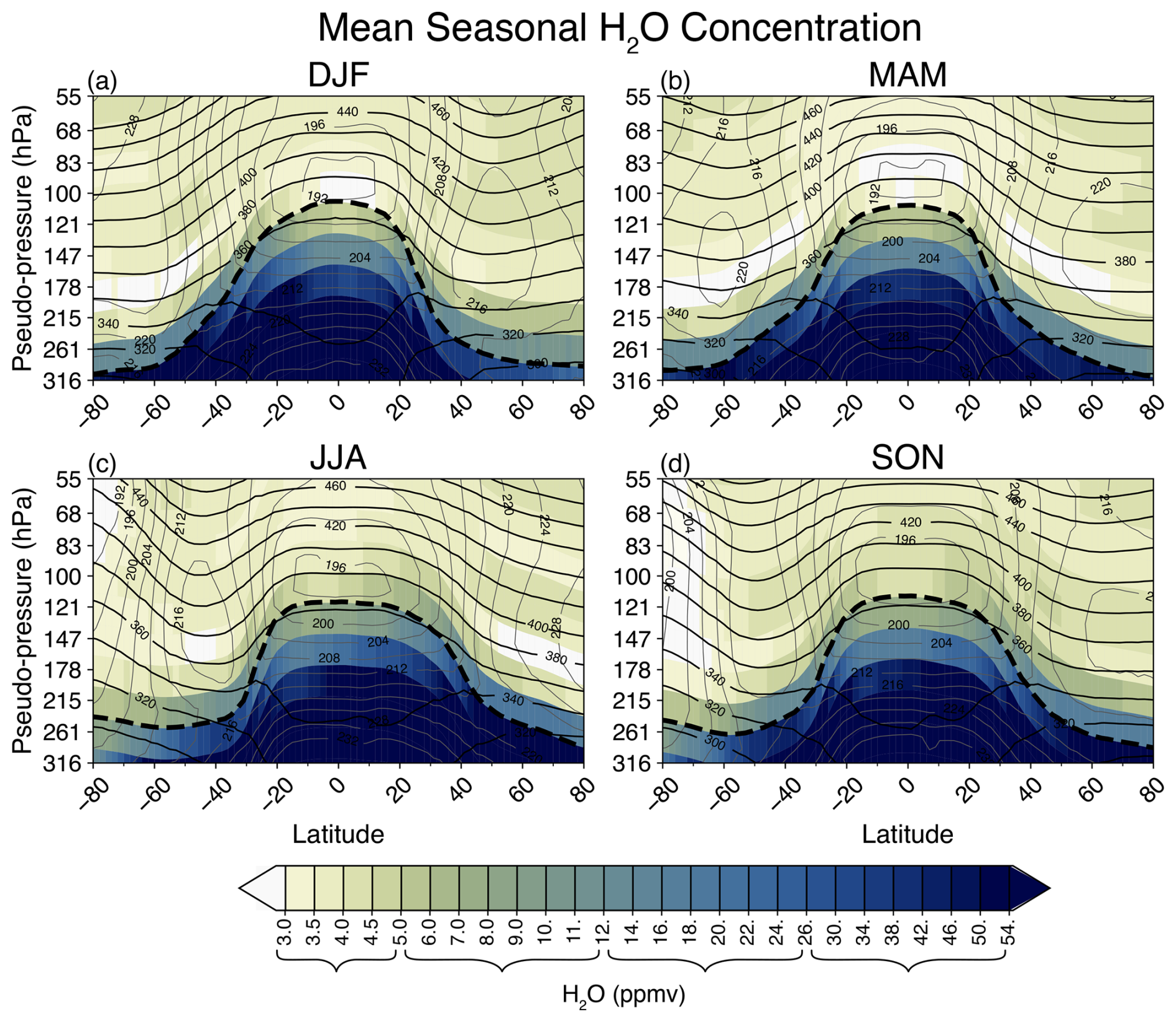
Figure 5 Zonally averaged cross sections of MLS H₂O data in tropopause-relative coordinates for (a) DJF, (b) MAM, (c) JJA, (d) SON. Color shading denotes the average MLS H₂O concentration, gray contours indicate temperature as observed by MLS, and black contours denote isentropes. The thick, dashed line is the average PTGT height for each season, calculated from MERRA-2 data. Curly brackets on the color bar delineate grouped value ranges corresponding to a non-uniformly spaced discrete scale.

The hemisphere-averaged annual cycle of lower stratospheric MLS water vapor concentrations in tropopause-following coordinates for both hemispheres is shown in Fig. 6a and c. These data represent area-weighted latitudinal and zonal averages poleward of 20° latitude, as described in Sect. 2.4, and are intended to represent mean hemispheric behaviors. As expected, there are strong vertical gradients across the tropopause. In both the Northern Hemisphere (NH) and Southern Hemisphere (SH) there is a clear annual cycle in upper tropospheric water vapor concentrations which peaks in hemispheric summer (labeled “B” in Fig. 6a and c), extending to the first layer above the tropopause (and weakly to the second layer). In the NH, water vapor concentration peaks at ∼16 ppmv in August in the first layer above the tropopause (∼1.25 km), while there is a peak of ∼7 ppmv in October that occurs ∼2.5 km above the tropopause. There is a similar summertime maximum in the SH for these lowest two stratospheric layers but with smaller amplitude. The dry layer associated with air originating near the tropical tropopause can be seen in Fig. 6a and c in both hemispheres (labeled “A” in Fig. 6a and c), occurring ∼3–4 km above the tropopause in February–August; this signal lags the seasonal H₂O minimum at the tropical tropopause by several months, and is coherent between hemispheres. This distinct seasonal cycle helps define the overworld influence on the water vapor concentrations in the extratropics. It follows that the height of this layer can be used as an upper boundary when defining the ExTL, providing a physically based definition to a layer that fluctuates in both space and time. Although not shown here, similar LMS H₂O seasonal cycles are observed in ACE data, but with limited resolution resulting from the 3-month temporal sampling.

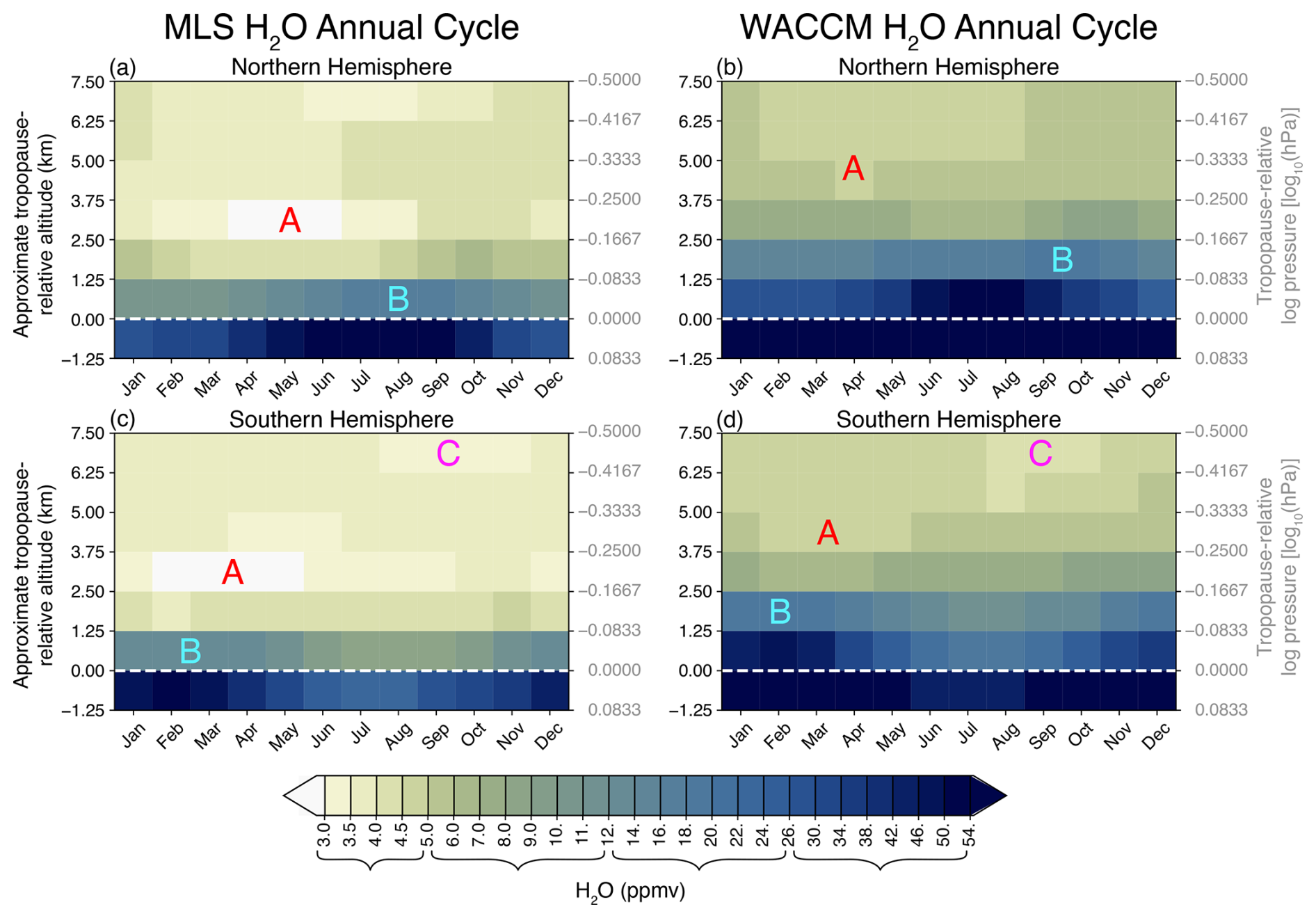
Figure 6 Average annual cycle of area-averaged H₂O concentrations in tropopause-relative coordinates for NH (a, b) and SH (c, d), showing results from MLS data (a, b) and WACCM simulation (b, d). The white horizontal dashed lines denote the tropopause level. The ordinate is tropopause-relative altitude. Letters denote specific features related to: (A) seasonal minimum due to overworld transport from tropics, (B) seasonal ExTL maximum tied to summer tropopause, and (C) minimum linked to Antarctic winter dehydration. Curly brackets on the color bar delineate grouped value ranges corresponding to a non-uniformly spaced discrete scale.

Corresponding extratropical LMS seasonal variations for WACCM are shown in Fig. 6b and d. In WACCM, the ExTL has higher H₂O concentrations than MLS and extends ∼1–2 km deeper into the stratosphere in both hemispheres, consistent with the time average biases seen in Fig. 4. Hence, the time average WACCM LMS H₂O biases are reflected in a thicker seasonally-evolving ExTL.

One further minor feature identified in the SH statistics in Fig. 6c and d is a minimum in H₂O in the SH during August–October, ∼5–7 km above the tropopause (i.e. geometric altitudes near 15–17 km) (labeled “C” in Fig. 6c and d). The altitude and timing of this feature suggest a relation to seasonal dehydration in the Antarctic polar vortex, where effects can spread outside the polar vortex in springtime (e.g., Rosenlof et al., 1997) and may be reflected in hemispheric mean H₂O.

3.3 Interannual Variability

To assess interannual variability and structure, the average monthly seasonal cycle is removed from the MLS time series to create deseasonalized anomalies, with time series for both hemispheres shown in Fig. 7. There is a distinct separation of patterns in the vertical structure occurring around ∼2.5 km above the tropopause in both hemispheres. Above 2.5 km tropopause-relative altitude there are interannual H₂O anomalies that are coherent between hemispheres. This variability is closely tied to overworld transport from the tropical tropopause source region, such that air is transported poleward into the extratropical LMS with a time scale of ∼2–4 months (e.g., Randel et al., 2024). In the ExTL below 2.5 km tropopause-relative altitude, the interannual patterns are different from above and variability is dominated by an apparent long-term decreasing trend in both hemispheres. This trend is further investigated in Sect. 3.4. Notably, even when the ExTL H₂O trend is removed, the vertical discontinuity in overworld and ExTL H₂O remains (see Fig. S1 in the Supplement).

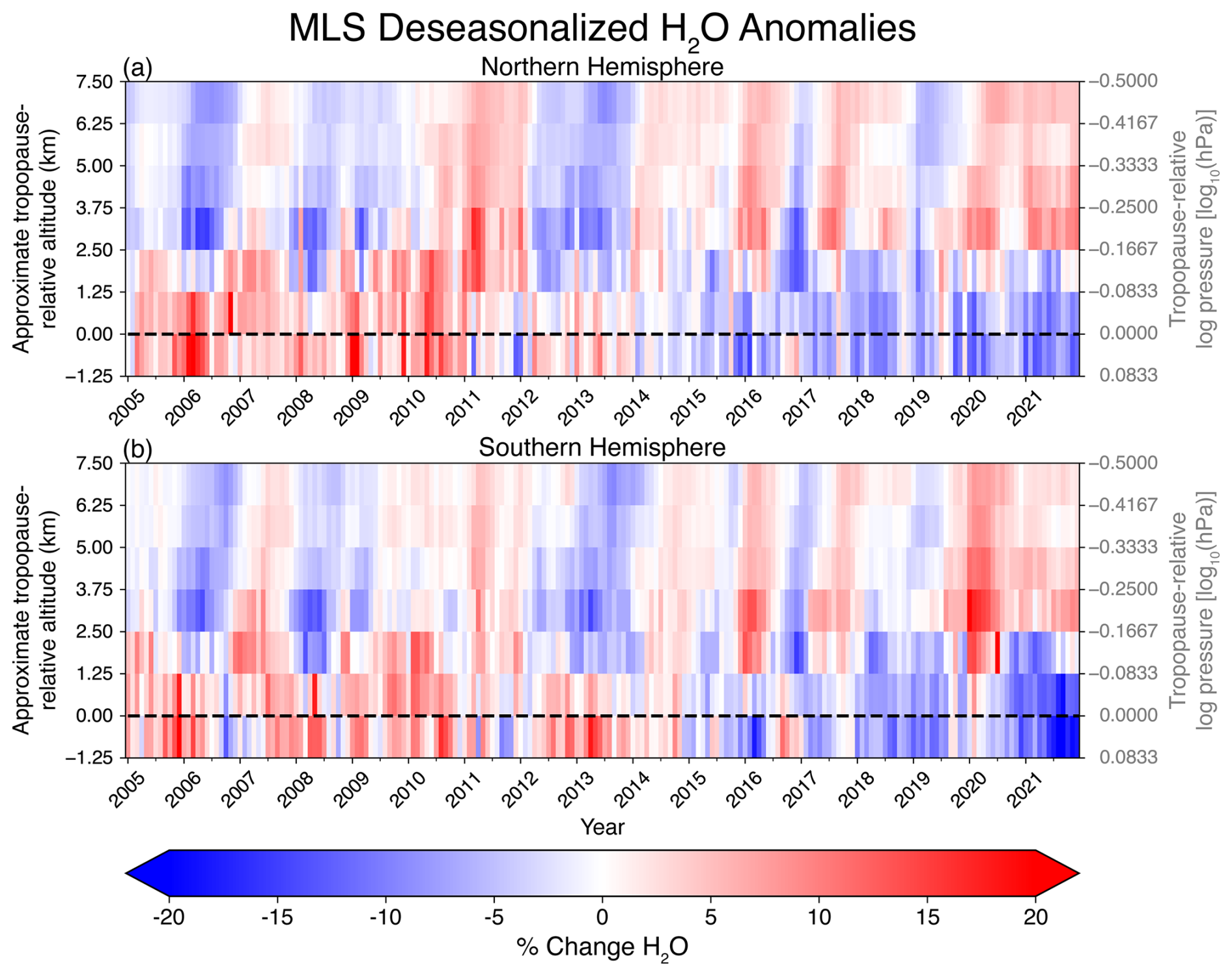
Figure 7 Time series of deseasonalized ExTL area-averaged MLS H₂O anomalies in tropopause-relative coordinates for (a) the NH and (b) the SH. Results at each level are expressed in percent deviations from the respective time mean background values.

A complementary perspective of the NH and SH H₂O anomalies in MLS data at several vertical levels is shown in the time series in Fig. 8. These show time series of overlaid NH and SH data to highlight correlated variability. Strong correlation (r=0.70) is found at the 3rd level (>2.5 km above the tropopause), with somewhat weaker correlation (r=0.41) over the 1.2–2.5 km layer. The first layer (0–1.25 km, within the ExTL) has weak interhemispheric correlation, aside from the strong trends.

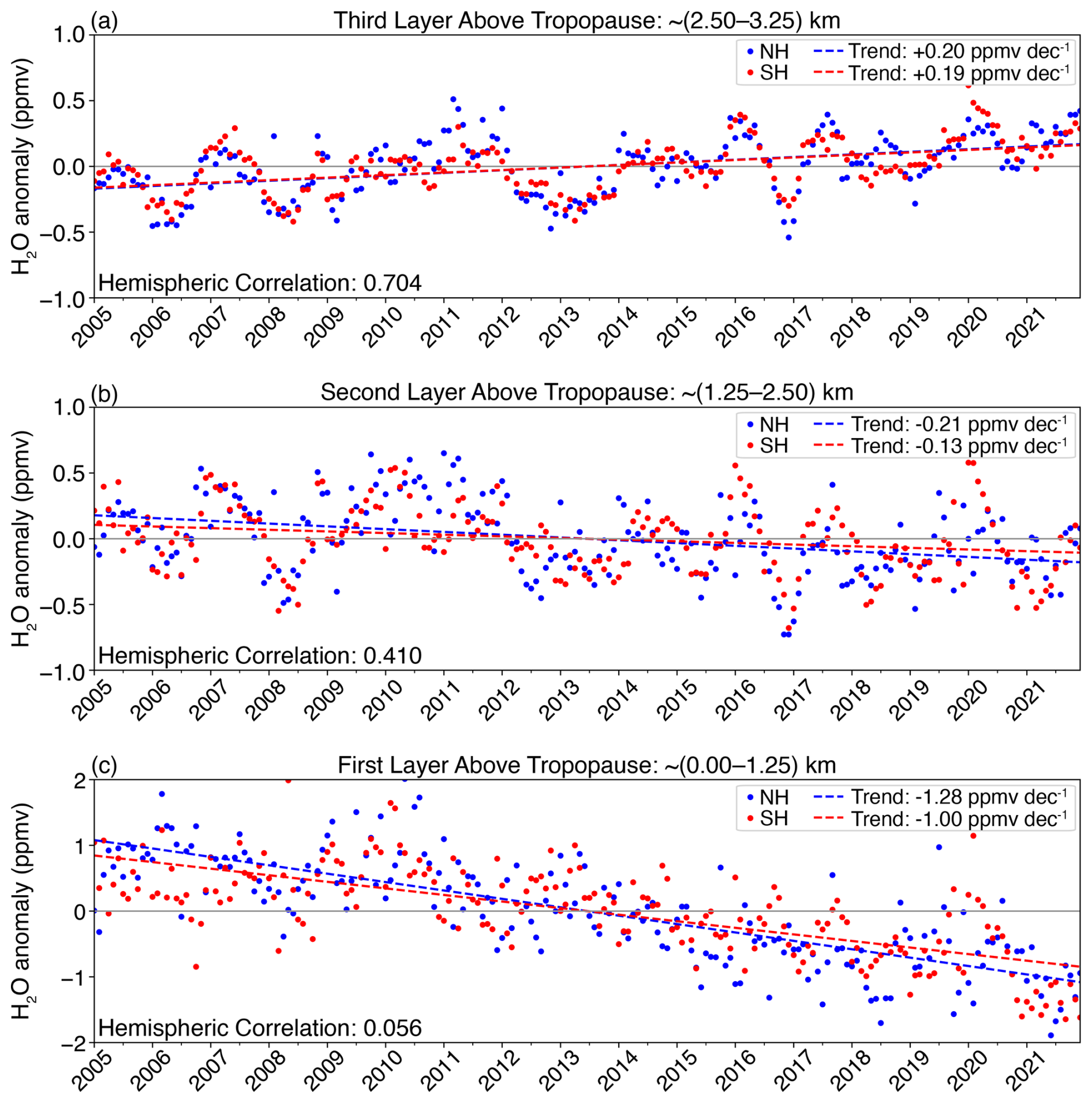
Figure 8 Time series of deseasonalized, tropopause-relative MLS H₂O anomalies in the three layers close to the tropopause (c to a). NH points are shown in blue, SH points in red, and the trend for each hemisphere is shown as a dashed line in the associated color. The correlation between hemispheres in the detrended time series is given in the bottom left corner of each panel.

Figure 9 provides additional evidence regarding the origin and transport of extratropical overworld H₂O anomalies, showing spatial correlations between deseasonalized and detrended water vapor anomalies to a reference point located near the tropical tropopause (83 hPa), with results in both geometric and tropopause-relative coordinates. At zero-time lag there are positive correlations centered in the tropics and extending poleward in a hemispherically symmetric pattern. The tropopause-relative calculations show strong correlations extending downward through the tropical upper troposphere, but this is an artifact of the tropopause-relative coordinates that is not observed in geometric coordinates. At a 2-month time lag, which is the general timescale of poleward transport from the tropics to the extratropical LMS (e.g., Randel and Park, 2019), the regions of highest correlations spread upward and further poleward in both coordinate systems. The tropopause-relative analysis shows higher extratropical correlations (above 0.6) and more vertically confined branches of positive correlations in the extratropical and polar regions, with the highest correlations occurring a few kms (∼100 hPa) above the tropopause. This is collocated with the dry layer of tropical origin shown in Figs. 5 and 6a–b, and quantifies the vertical profile of overworld transport from the tropics that defines the effective top of the ExTL. Parallel analysis of the WACCM simulation is given in Fig. S2.

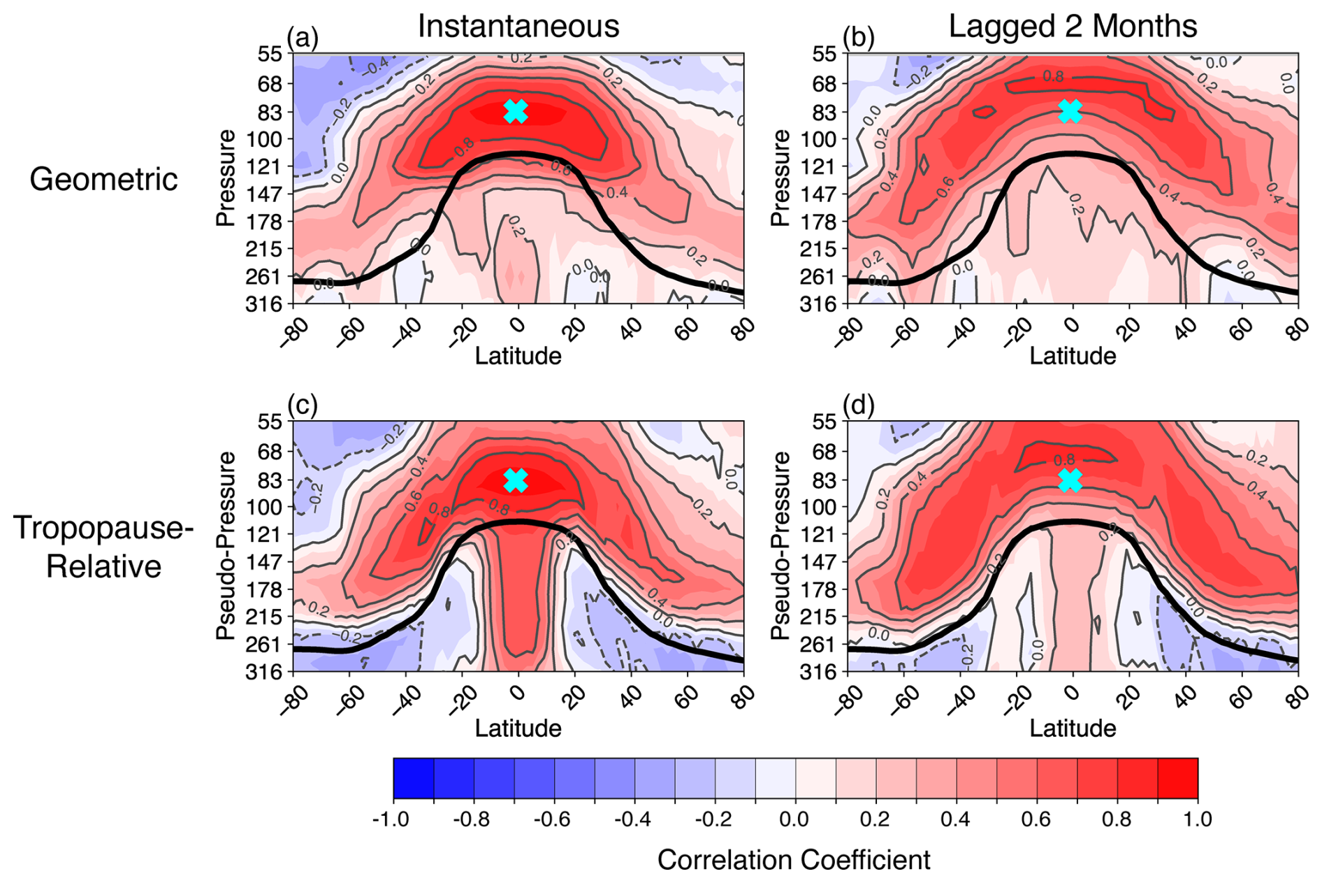
Figure 9 Correlation of deseasonalized MLS water vapor anomalies at each point with the anomaly near the tropical tropopause (teal X; 83 hPa). Correlations are shown in both (a, b) tropopause-relative and (c, d) geometric coordinate systems at (a, c) zero-time lag and (b, d) a two-month time lag.

The observed distinction between overworld and ExTL, as identified by their vertical structure and temporal behavior, raises the question of whether similar behavior occurs for other trace gases. Identical to the analysis conducted for Fig. 7, deseasonalized ozone anomalies from MLS are shown in Fig. 10. In contrast to the H₂O results, there is a coherent vertical structure in each hemisphere in the ozone anomalies that extends from the overworld down to across the tropopause, with no evidence of discontinuity across the ExTL (although the background amounts of ozone changes significantly). Given that H₂O and ozone both exhibit large gradients across the tropopause, one might expect a similar behavior in the vertical continuity (or lack thereof) in the two trace gases. However, the exact vertical tropopause-relative locations and magnitudes of such gradients vary substantially between H₂O and ozone, such that H₂O experiences a far more extreme transition across the extratropical tropopause than ozone (see Fig. 11 in Tinney and Homeyer, 2021). The distinct behavior for H₂O compared to ozone is therefore realistic due to the large reservoir of H₂O below the tropopause together with the source of overworld variability in the tropics. Additionally, there is little correlation in the ozone anomalies between the NH and SH because the location of the strongest ozone gradient exists well above the tropopause (∼2–7 km), where variability is more sensitive to extratropical downwelling which is mostly independent between hemispheres.

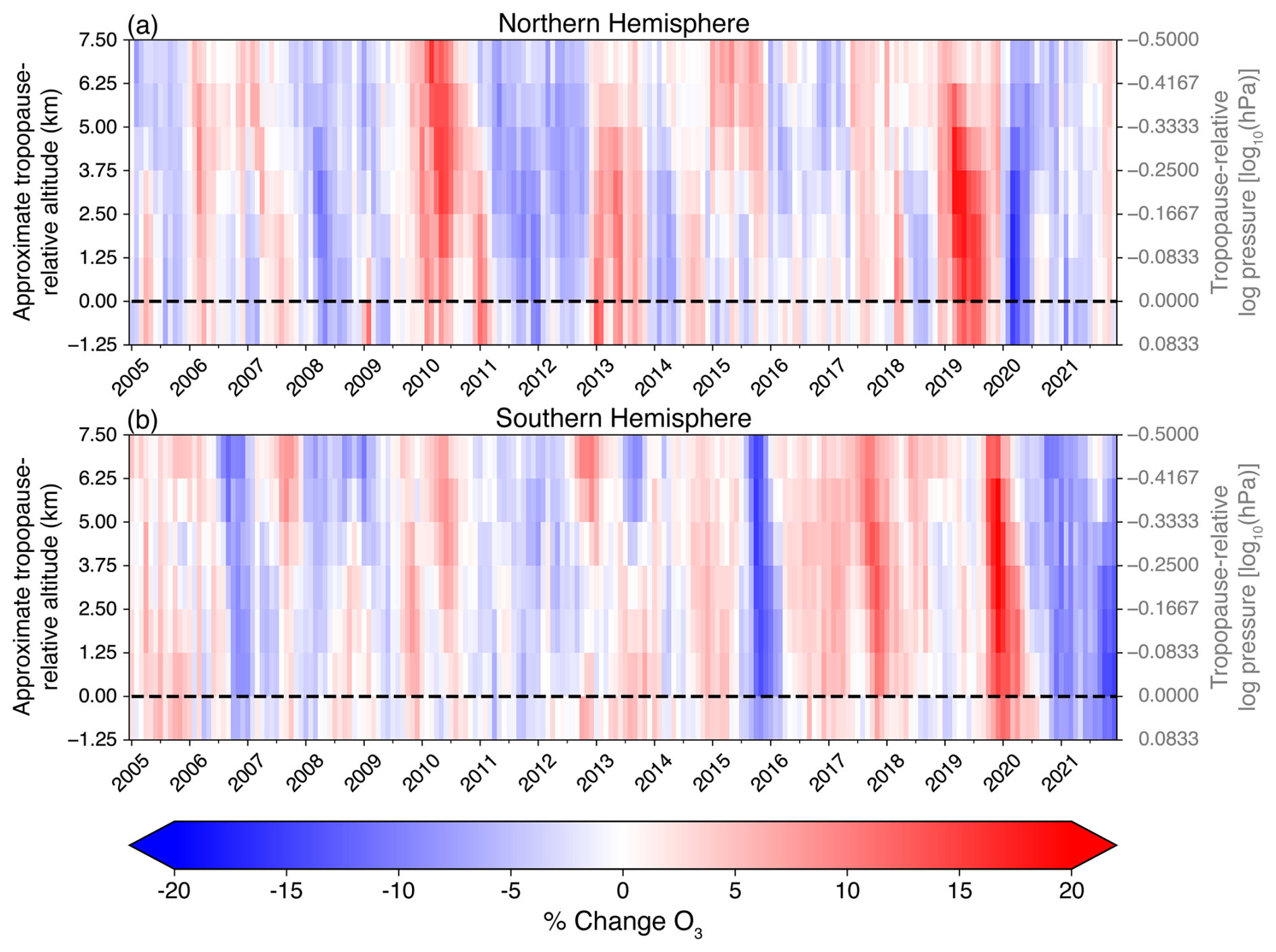
Figure 10 Time series of deseasonalized ExTL area-averaged MLS ozone anomalies for (a) the NH and (b) the SH. Results at each level are expressed in percent deviations from the respective time mean background values.

For comparison with MLS, we also examine deseasonalized water vapor anomalies in ACE and WACCM in Fig. 11 and the ACE and WACCM versions of Fig. 7 are given in Figs. S3 and S4. The broad, hemispherically coherent interannual variability seen in MLS above ∼2.5 km tropopause-relative altitude is also present in the ACE and WACCM datasets (Fig. 11a–b). ACE reproduces the timing and vertical extent of H₂O anomalies seen in MLS but with greater noise and reduced amplitude, likely related to the latitudinally-varying sampling across seasons. Despite this limitation, the sign and phase of anomalies generally match MLS, supporting consistency between observational datasets. WACCM also matches the overall structure and phase of the overworld anomalies seen in MLS, which is expected due to the prescribed tropical tropopause temperatures used in the specified dynamics run. However, the magnitude of the WACCM variability is substantially larger than MLS, perhaps due to the vertical smearing (∼3 km) inherent in the MLS data. While the overworld H₂O variations are consistent among MLS, ACE, and WACCM, the ExTL variations are markedly different between datasets as neither ACE nor WACCM displays the negative trend observed from MLS in the ExTL layer (Fig. 8c). These comparisons are explored further in Sect. 4. Importantly, the magnitude of the trend in the MLS ExTL makes investigation of dataset comparisons of other variability in this layer infeasible.

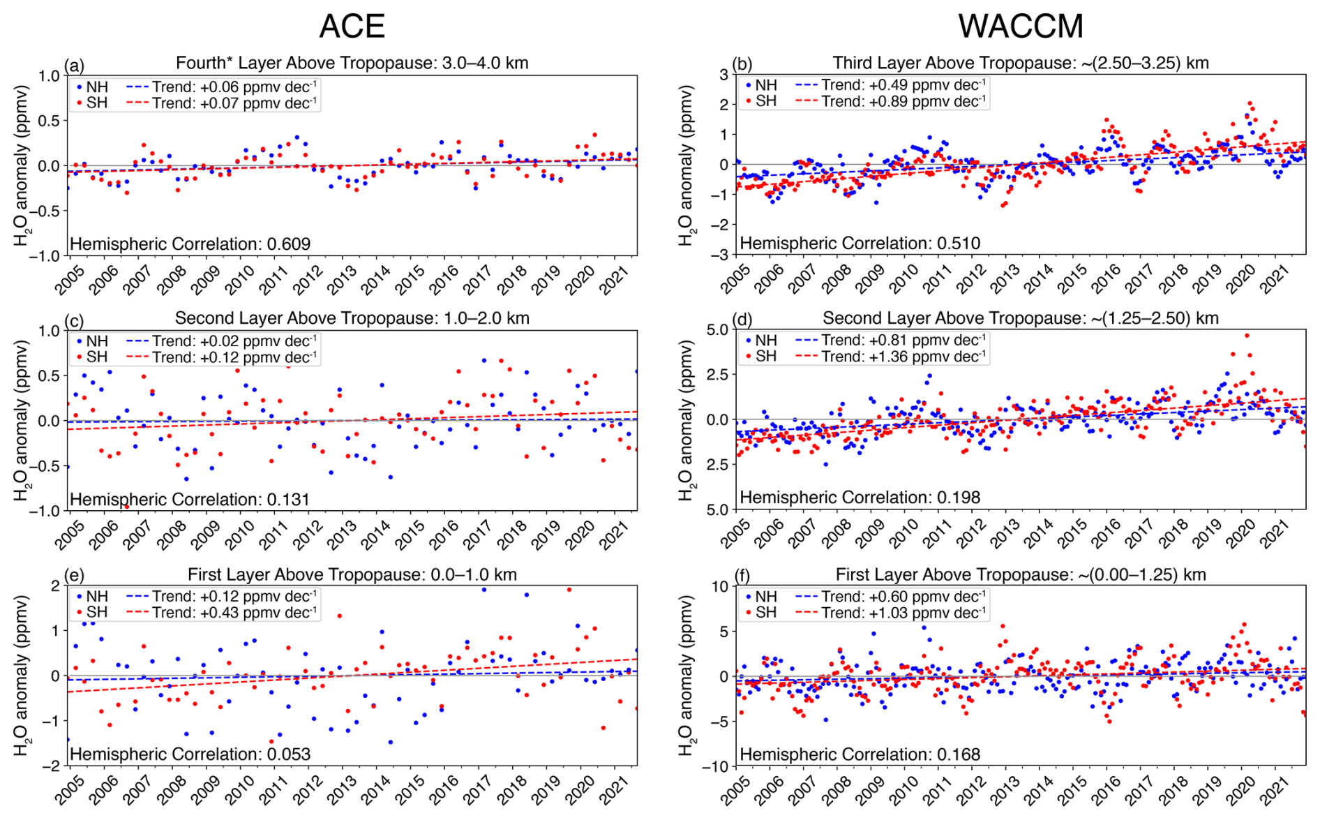
Figure 11 Time series of deseasonalized, tropopause-relative H₂O anomalies in three layers close to the tropopause (bottom to top) for ACE observations (a, c, e) and WACCM simulation (b, d, f). The format is the same as the MLS results in Fig. 8, but note the different ordinate for WACCM compared to MLS and ACE.

The vertical variation of the correlation between water vapor anomalies in the NH and SH in each dataset is explored in Fig. 12. The hemispheric correlations in MLS, ACE, and WACCM exhibit a similar vertical structure, with a minimum in the first or second layer above the tropopause, and a maximum that occurs around 4–5 km above the tropopause. Throughout the vertical profile, hemispheric correlation in ACE is consistently 0.1–0.3 smaller than MLS. This is likely a reflection of the sparser sampling of the ACE dataset. Comparisons of seasonal means between hemispheres can remain sensitive to the latitudinal distribution of contributing profiles, thereby adding additional sources of variability and reducing the correlation coefficient between hemispheres. The hemispheric correlation in WACCM above 5 km tropopause-relative altitude is nearly identical to MLS, which is expected due to specified dynamics and prescribed tropopause temperatures in the model accurately reflecting stratospheric overworld behavior. Below 5 km tropopause-relative altitude, however, the values of the correlation coefficients in WACCM are systematically smaller than MLS. This behavior may be a signature of the moist LMS bias and deeper extent of the ExTL in WACCM (e.g., Fig. 6).

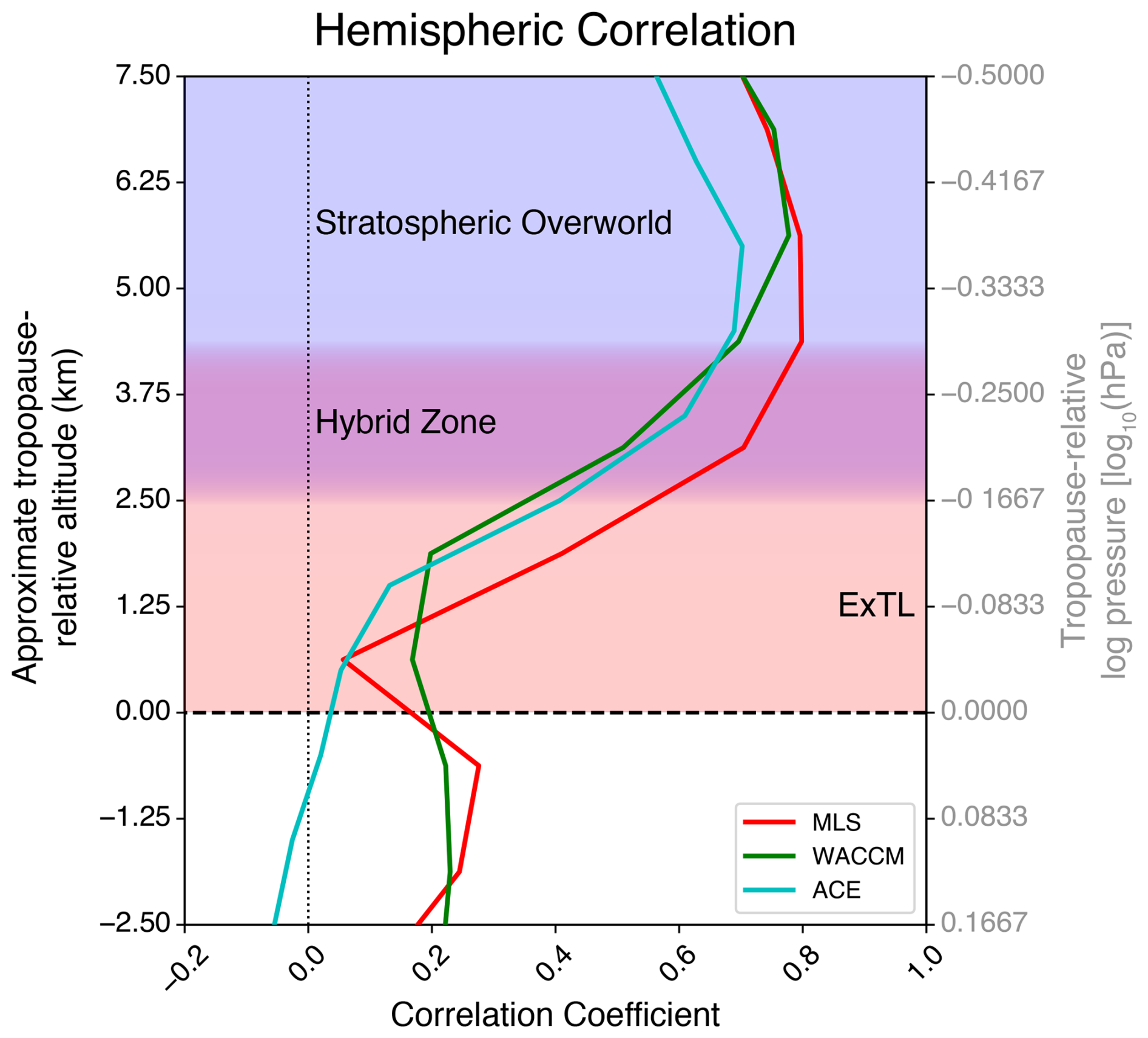
Figure 12 Correlation coefficient between NH and SH extratropical detrended and deseasonalized H₂O anomalies on tropopause-relative levels for MLS (red), WACCM (green), and ACE (teal). Subjectively identified regions are depicted by background shading for the ExTL (red), the overworld (blue), and a hybrid zone (purple).

The commonality of higher hemispheric correlation above 4 km tropopause-relative altitude in all three datasets demonstrates that hemispheric symmetry is a robust signature of the stratospheric overworld, resulting from a common stratospheric entry point and similar transport times of the lower branch of the BDC (e.g., Garny et al., 2024; Randel et al., 2024). In diagnosing the vertical structure of the lower stratosphere, hemispheric symmetry and correlation can provide a physical indicator of the separation between the stratospheric overworld, the ExTL, and the hybrid region in between (Fig. 12).

3.4 Trends and other sources of variability in the ExTL

The dominant variability in the ExTL in MLS H₂O data is a downward trend (Fig. 8c). However, this trend is not evident in either ACE observations or WACCM simulation (Fig. 11). Here we examine large-scale variability and trends in the global data sets to identify coherent structures and systematically evaluate trends. We conduct a standard multivariate linear regression to the H₂O time series at each point and include terms representing a linear trend, ENSO, and the QBO (using two orthogonal time series) to isolate their respective contributions to observed variability (e.g., Godin-Beekmann et al., 2022):

$$\begin{array}{}\text{(1)}& \begin{array}{rl}y\left(t\right)& ={\mathit{\beta }}_{\mathrm{0}}+{\mathit{\beta }}_{\mathrm{1}}t+{\mathit{\beta }}_{\mathrm{2}}\mathrm{ENSO}\left(t\right)+{\mathit{\beta }}_{\mathrm{3}}{\mathrm{QBO}}_{\mathrm{1}}\left(t\right)\\ & +{\mathit{\beta }}_{\mathrm{4}}{\mathrm{QBO}}_{\mathrm{2}}\left(t\right)+\mathit{\epsilon }\left(t\right)\end{array}\end{array}$$

where β₁t represents the trend term and ε(t) is the residual. The ENSO and QBO proxies are taken from the NOAA Physical Sciences Laboratory Multivariate ENSO Index (MEI) and the NASA Goddard Space Flight Center QBO datasets, respectively. Statistical significance of regression coefficients was assessed using a two-sided Student's t-test with a p<0.05 significance threshold. To account for serial autocorrelation in the regression residuals, an effective sample size for each dataset was calculated as:

$$\begin{array}{}\text{(2)}& N_{\mathrm{eff}}=N{\displaystyle \frac{\mathrm{1}-r_{\mathrm{1}}}{\mathrm{1}+r_{\mathrm{1}}}}\end{array}$$

where N is the number of observations and r₁ is the lag-1 autocorrelation of the regression residuals. The effective sample size was then used when computing the standard errors and resulting p-values of the regression coefficients. Results are calculated for both geometric and tropopause-relative coordinates.

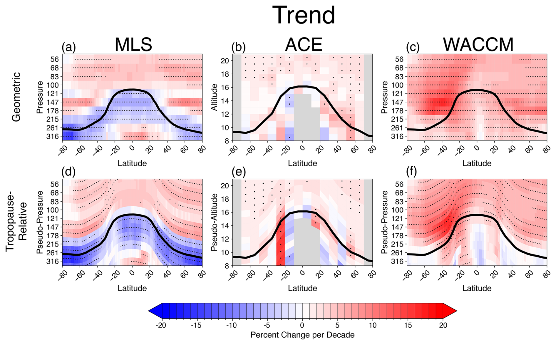
Figure 13 Latitude-height sections of H₂O trends for MLS data (a, d), ACE data (b, e) and WACCM simulation (c, f), calculated in geometric coordinates (a–c) and tropopause-relative coordinates (d–f). Results are shown in % per decade, calculated with respect to the respective long-term background values. Stippling denotes regression coefficients significant at the p<0.05 level. ACE data is masked in gray where fewer than half of timesteps have sufficient observations.

Results of the trend calculations are shown for all three data sets in Fig. 13. Trends in the overworld are generally positive in all data, reflecting a slight increase in cold point temperature over the data record 2005–2021. Similar positive stratospheric H₂O trends over this time period have been shown in Sheese et al. (2025), Tao et al. (2023), Konopka et al. (2022), and Yu et al. (2022). In contrast, H₂O trends in the troposphere and ExTL of both hemispheres are very different among the datasets. MLS exhibits negative trends in the global upper troposphere and ExTL regions, with patterns that generally follow the global tropopause structure. The trends are slightly more negative in tropopause-relative coordinates, reflecting the slight rise of the tropopause over this period (e.g., Ladstädter et al., 2025; Meng et al., 2021), which acts to reduce H₂O values in the tropopause region, all else being equal. However, these systematic, large-scale negative trends derived from MLS data are not evident in either ACE observations or WACCM simulation, and these differences question the reality of the MLS trend results in the troposphere and ExTL, as discussed further below.

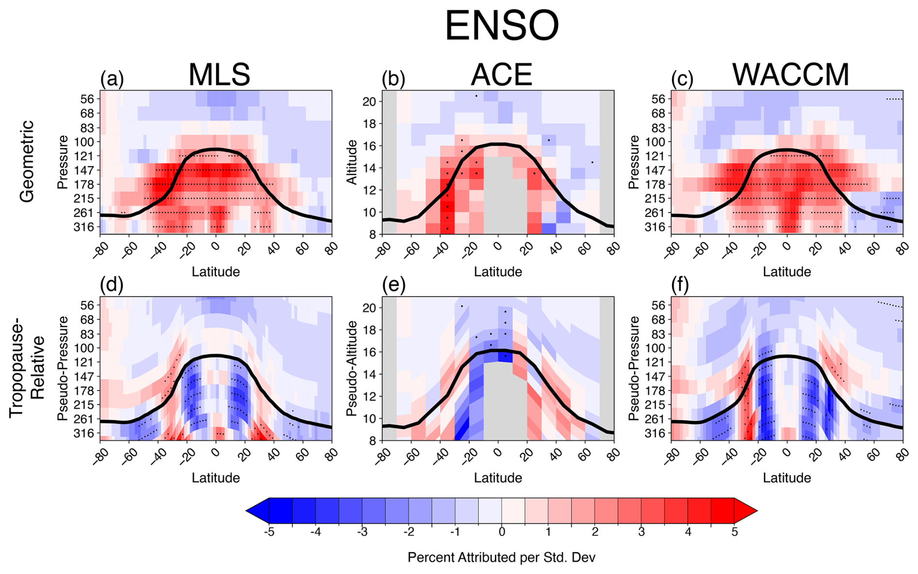
Figure 14 Latitude-height sections of ENSO regression fit to H₂O for MLS data (a, d), ACE data (b, e) and WACCM simulation (c, f), calculated in geometric coordinates (a–c) and tropopause-relative coordinates (d–f). Results are shown in % per normalized ENSO index, calculated with respect to the respective long-term background values. Stippling denotes regression coefficients significant at the p<0.05 level. ACE data is masked in gray where fewer than half of timesteps have sufficient observations.

Regression fits for ENSO variability are shown in Fig. 14. In general, H₂O is expected to follow temperature changes throughout the troposphere (from the Clausius-Clapeyron relationship), so that positive H₂O ENSO regression patterns are expected in the troposphere following the well-known positive zonal mean temperature changes for ENSO (e.g., Li et al., 2024; Johnston et al., 2022). This positive ENSO signal is observed in MLS, ACE, and WACCM geometric coordinate results (top row in Fig. 14), with patterns covering the tropical upper troposphere and extending across the tropopause to higher latitudes in both hemispheres. Hence, ENSO is a significant component of ExTL H₂O variability. However, the broad-scale ENSO signature is much less coherent (and insignificant) in tropopause-relative coordinates (bottom row of Fig. 14), because the ENSO-related changes in tropopause height confuse the signal in the tropics.

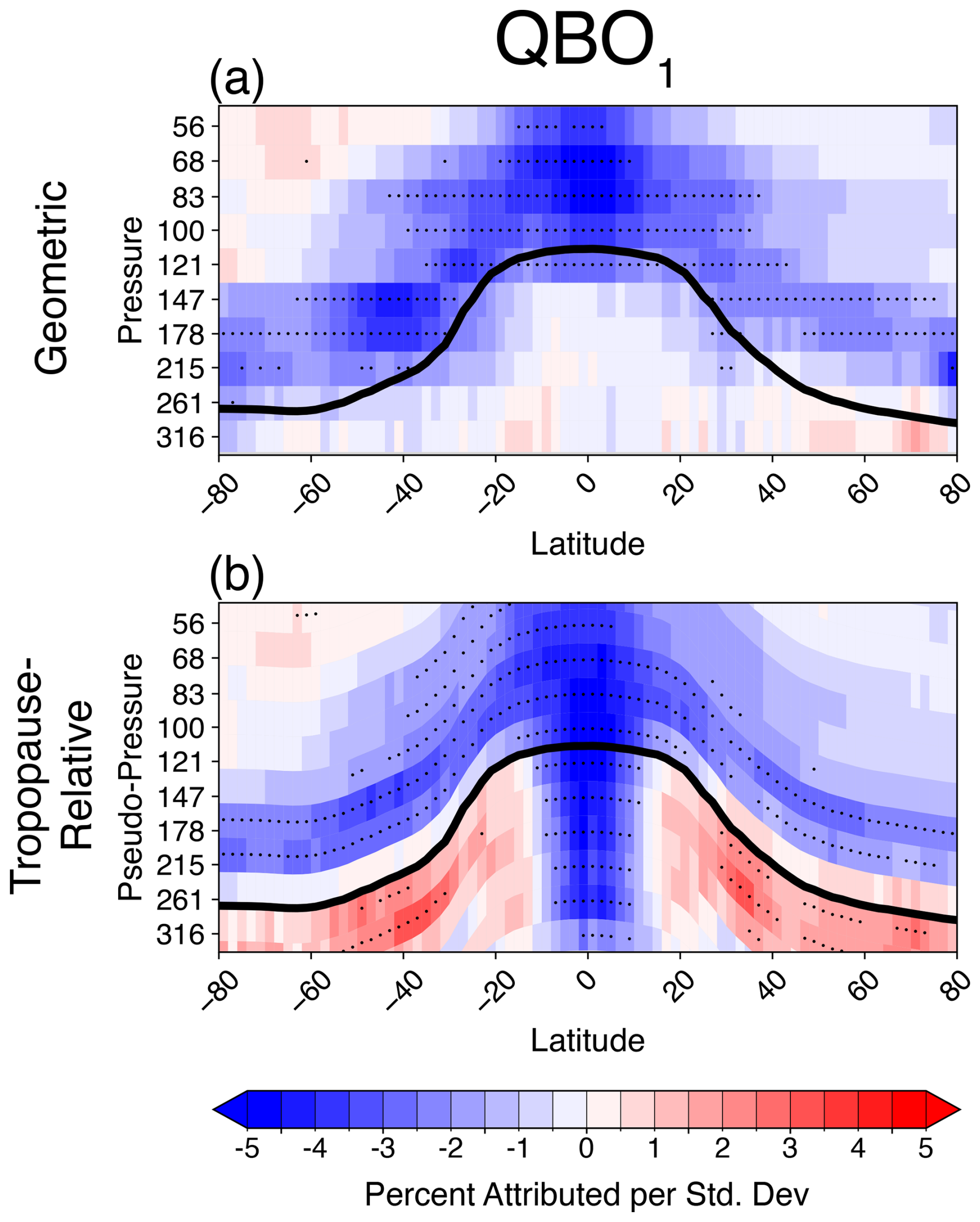
Figure 15 Latitude-height sections of QBO1 regression fit to H₂O for MLS data, calculated in geometric coordinates (a) and tropopause-relative coordinates (b). Results are shown in % per normalized QBO1 index, calculated with respect to the respective long-term background values. Stippling denotes regression coefficients significant at the p<0.05 level.

The global QBO1 pattern in MLS H₂O data is shown in Fig. 15. The QBO1 index is negatively correlated with tropical cold point temperature (e.g., Randel et al., 2015) and this produces a negative correlation with H₂O in the tropics and global lower stratosphere (i.e. overworld). Results in tropopause-relative coordinates show sharper and more vertically stratified patterns that delineate overworld influence and ExTL structure. QBO1 patterns in the troposphere in Fig. 15b (negative values over the equator and positive below the tropopause in extratropics) reflect the influence of the QBO on tropopause height, and are artifacts of the coordinate system. Similar QBO regression results are found in ACE and WACCM data and are not shown here. QBO2 regression coefficients have little impact on the CPT and hence have less impact on H₂O (not shown here).

4 Summary and discussion

This work has examined the variability and vertical structure of H₂O in the extratropical lower stratosphere, using geometric and tropopause-relative coordinate analysis of monthly mean satellite data and WACCM global model simulations. The use of tropopause-relative coordinates reduces seasonal and interannual variance in the ExTL regions and sharpens the geophysical structure evident in the data. However, tropopause-relative coordinates are not as useful in the deep tropics, as they introduce additional H₂O variance in the upper troposphere and can confuse interpretation of results (e.g. the ENSO regressions in Fig. 14). The ExTL (transition region in extratropics) is identified in the observed H₂O seasonal and interannual anomaly patterns to span the first 2.5 km above the tropopause; we note that this result should be interpreted considering the approximate 3 km vertical resolution of the MLS and ACE satellite retrievals. However, this value is consistent with the depth of the ExTL diagnosed from aircraft and balloon measurements in midlatitudes (e.g., Gettelman et al., 2011; Pan et al., 2004; Hoor et al., 2002). H₂O variability above the ExTL (in the stratospheric overworld) is correlated between hemispheres, identifying a source region for both hemispheres near the tropical tropopause (Fig. 12). In the ExTL and below, H₂O variability is tied to tropospheric H₂O and is uncorrelated between the NH and SH. While ENSO is one source of global-scale H₂O variability that extends from the tropical upper troposphere across the tropopause into the LMS (Fig. 14 in geometric coordinates), more generally the ExTL is independent between the NH and SH. As a note, LMS ozone interannual variability is very different from H₂O, with little coherence between hemispheres and no change in behavior of anomalies across the ExTL.

The WACCM simulations using observed meteorological fields show much of the same LMS structure and variability as the satellite observations, although direct comparisons highlight a strong positive model H₂O bias in the LMS. This behavior was noted in Charlesworth et al. (2023) and shown to be a feature of other global models (e.g. CMIP6). Charlesworth et al. (2023) diagnose a cause of overly diffusive transport as one source of this model bias, which ends up impacting LMS temperatures and global circulations. The wet LMS bias in WACCM is found in seasonal (Fig. 6) and interannual H₂O anomalies (Fig. 11f) across the ExTL, and the ExTL is approximately 1–2 km deeper in WACCM compared to satellite data (Fig. 12).

MLS H₂O observations show strong negative trends in the global upper troposphere that extend across the tropopause and dominate variability in the ExTL (e.g. Fig. 8c). The global trend patterns (Fig. 13a) approximately follow the region with background H₂O values on the order of 300 ppmv in the troposphere extending down to ∼20 ppmv in the ExTL. These trends are evident in geometric coordinates and are slightly enhanced in tropopause-relative coordinates due to the long-term rise of the extratropical tropopause. The negative global-scale H₂O trends in MLS data are not evident in ACE observations or in our specified dynamics WACCM simulations, and they are not expected due to the generally increasing background tropospheric temperatures over 2005–2021 (as quantified by the WACCM specified dynamics calculations). The MLS H₂O decreases in the tropical upper troposphere seen in Fig. 13 also disagree with other infrared and microwave satellite observations, which show consistent specific humidity increases in this region over the recent decades (e.g., John et al., 2025; Allan et al., 2022). Likewise, results for ERA5 reanalysis show moistening of the tropical upper troposphere since 2000 (e.g., Li et al., 2024; Allan et al., 2022; Konopka et al., 2022). As a result, we view the negative trends with a skeptical eye, as their absence in independent observations and model simulations raises the possibility of a retrieval-related contribution to the MLS v5.x trends that should be further investigated. Issues in the long-term stability of previous versions of the MLS H₂O (a spurious positive drift in v4.x) measurement have been identified (Hurst et al., 2016) and partially ameliorated for v5.x, but the MLS team recommends continued caution when using the MLS record to investigate long-term H₂O trends (Livesey et al., 2021, 2022).

However, we emphasize here that there are several limitations that should be considered when interpreting these results. Namely, the effective vertical resolution of the satellite H₂O retrievals is comparable to the diagnosed depth of the ExTL, which makes disentangling changes in the upper troposphere from the lower stratosphere challenging. In addition, the 2005–2021 analysis period is relatively short for distinguishing a persistent long-term trend from lower-frequency variability. Finally, the WACCM comparison provides a useful physical constraint on the observed variability, but differences between the model and observations may also reflect limitations in the representation of transport and mixing in the LMS, rather than necessarily indicating an observational error.

In summary, this study demonstrates that H₂O variability can help distinguish the extratropical transition layer from the stratospheric overworld. Above ∼ 2.5 km above the tropopause, the strong correlation between the hemispheres and connection to the tropical tropopause source region are consistent with transport by the Brewer–Dobson circulation. Within the ExTL, H₂O variability is less correlated between hemispheres, suggesting a greater influence from local and regional troposphere–stratosphere exchange processes. The agreement among MLS, ACE-FTS, and WACCM in the overworld suggests that these features of H₂O variability are robust. Alternatively, the apparent negative trend in MLS ExTL H₂O concentration stands in contrast to other observational and modeling results which highlights the difficulty of identifying long-term changes in this region. Continued evaluation with independent observations and improved representation of LMS transport in models is needed for better understanding how the ExTL responds to changes in the troposphere and stratospheric circulation.