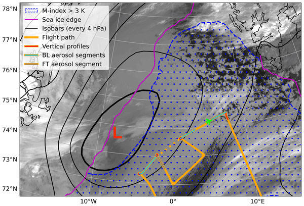
A closed-to-open cell mixed-phase cloud transition observed over the Nordic Seas under high aerosol loading and strong surface fluxes

Closed-to-open cell mixed-phase cloud transitions within marine cold air outbreaks remain poorly understood despite their importance to high-latitude climate. The Cold-Air outbreak Experiment in the Sub-Arctic Region (CAESAR) research aircraft sampled a cold and polluted closed-to-open cell transition with cloud-top temperatures below −20 °C and upstream cloud condensation nuclei concentrations surpassing 600 cm⁻³. The aerosol likely originates from Siberian industrial emissions. As the boundary layer deepens prior to and across the transition, driven by strong turbulent surface fluxes and aided by a weakening cloud-top inversion, aerosol number concentrations decrease and supercooled droplet sizes increase, causing ice particles to shift from primarily vapor depositional growth towards riming. Precipitation shafts within open-cells contain abundant large graupel (>5 mm diameter) with liquid-equivalent precipitation intensities reaching 3 mm h⁻¹. Ice precipitation co-exists with lidar-observed surface cold pools, modulated by entrainment events, juxtaposed with surface-based plumes of warm moist air. Updrafts support liquid water production along convergence boundaries at the upwind cold pool edge. Nonetheless, strong buoyancy fluxes exceeding 200 W m⁻² prevent sub-cloud decoupling. Ice particle number concentrations increase tenfold across the transition, surpassing 10 L⁻¹ within open-cells, more than 1000× ice nucleating particle number concentrations. Given that cloud temperatures are too cold for Hallett-Mossop rime splintering, this indicates the importance of other secondary ice production mechanisms. This case expands the observations needed to better understand mixed-phase Arctic cloud processes.

1 Introduction

Marine cold air outbreaks (MCAOs) are extreme weather events that occur when a cold air mass advects over open water, with strong winds supporting intense surface sensible and latent heat fluxes capable of reaching 1000 W m⁻² over open water near the Arctic sea ice (Papritz et al., 2015; Papritz and Spengler, 2017). Mid- to high-latitude MCAOs often contain mixed-phase clouds (Abel et al., 2017; Geerts et al., 2022; Murray-Watson et al., 2023; Wendisch et al., 2024; Chellappan et al., 2024), initially organized as convective rolls or “cloud streets” (Brümmer and Pohlmann, 2000; Young et al., 2002). As surface turbulent fluxes and wind shear weaken and the MCAO ages, the convective rolls can evolve into closed-cell stratocumulus, transitioning into open-cells with further fetch (McCoy et al., 2017). These transitions impact the cloud cover, which in turn impacts the radiative budget (e.g., Narizhnaya and Chernokulsky, 2024) that the high-latitude climate is sensitive to. MCAOs can also spawn polar lows: small, intense and unpredictable cyclones (Newman et al., 2025) that are consequential for coastal communities and shipping. The MCAO lifecycle is thus impactful to both high-latitude weather and climate.

MCAO cloud transitions are to first order dictated by environmental variability in surface fluxes and free tropospheric (FT) conditions, summarized by the marine cold air outbreak index (Fletcher et al., 2016). For example, mid-latitude air mass trajectories located under lower FT temperatures and weaker subsidence will transition sooner to open-cells (Tornow et al., 2023). Numerical weather prediction models and reanalyses can depict the synoptic patterns that generate MCAOs. The models and reanalyses nevertheless struggle to represent the dynamic, thermodynamic, and microphysical processes and aerosol-cloud interactions that inform the transition on the sub-kilometer scale (Field et al., 2017; Juliano et al., 2024, 2026).

In warm stratocumulus, precipitation is a necessary condition for cloud transitions and provides a useful metric that can be compared between models and observations (Wood et al., 2011). The precipitation helps drive density-driven gust fronts that help initiate new updrafts by developing surface cold pools through evaporation (Zuidema et al., 2017). In the trade-wind regions, a rain rate threshold of 2 mm h⁻¹, averaged over the rain's catchment area, corresponds well to downdrafts of air with equivalent potential temperatures (θ_e) lower than their surroundings (Barnes and Garstang, 1982). These support moderate updraft velocities (<2 m s⁻¹) that can initiate new convection (Zuidema et al., 2012). Whether such relationships also hold for Arctic MCAOs is, to our knowledge, not known, as cold pool behavior has not been extensively assessed in suppressed environments with strong surface turbulent fluxes. Gentine et al. (2016), in a modeling study intended for the lower-latitudes, find strong, interactive surface fluxes induce smaller but more numerous cold pools with weaker gust front velocities, compared to simulations with horizontally-homogenized surface fluxes. One recent Arctic-related study finds most of the variance in flight-level turbulent fluxes occurs at scales <5 km for a separate MCAO case (McGinnity et al., 2026). The modeling of sub-cloud distributions of vertical velocity, moisture and temperature in marine environments is still challenging, however, even in warmer, better-documented environments (Zhu and Zuidema, 2009; Chandra et al., 2018; Poydenot et al., 2026).

Precipitation is also altered by aerosols. Higher cloud condensation nuclei concentrations (N_CCN) can reduce droplet size, delaying the transition to lower cloud cover (Murray-Watson et al., 2023). Smaller drop sizes delay precipitation formation, well-accepted by now for liquid-only transitions (Wood et al., 2011; Yamaguchi and Feingold, 2015; Smalley et al., 2022; Sansom et al., 2026). Smaller drops evaporating closer to the cloud base help destabilize the sub-cloud layer, better coupling the cloud to the surface turbulent fluxes (Feingold et al., 1996; Sarkar et al., 2020). In mixed-phase clouds, smaller drops also rime less efficiently (Khain et al., 2001; Wang and Ji, 2000), which also helps maintain the cloud. More of the ice particle growth, especially at ice-saturated temperatures near −15 °C, is likely to occur through the Wegener-Bergeron-Findeisen (WBF) process (Wegener, 1911; Bergeron, 1935; Findeisen, 1938), wherein smaller drops evaporate readily, and the vapor is deposited on neighboring ice particles. Ice growth through vapor deposition can also occur in water-saturated updrafts, capable of producing new cloud droplets (Pinsky et al., 2015). Where larger drops support riming, the larger rimed ice particles fall faster than the pristine dendrites and can more easily deplete the cloud liquid (Tornow et al., 2021). Variations in ice-nucleating particle concentrations (N_INP) furthermore compete with N_CCN: some modeling suggests higher N_INP facilitate earlier cloud deck breakups (Wu et al., 2025), but observations over northern Alaska indicate that if higher N_INP are accompanied by elevated N_CCN, the ice mass production is reduced (Lance et al., 2011; Norgren et al., 2018). Observational analysis within sub-Arctic MCAOs suggests N_INP may increase as more open water becomes available, although the INP source remains unclear (DeMott et al., 2025). The ice particle number concentrations (N_i) can also increase through secondary ice production (SIP) processes over time, most convincingly at cloud temperatures $>-\mathrm{10}$ °C (Abel et al., 2017; Chellappan et al., 2024; Schafer et al., 2024; Biggart et al., 2026; Pearson et al., 2026). Sullivan et al. (2017), in a modeling study, found that moderate updrafts (2–3 m s⁻¹) are best able to support SIP, as weaker updrafts primarily deplete liquid through precipitation, and stronger updrafts do not allow sufficient hydrometeor growth.

High-quality in situ observations of Arctic mixed-phase cloud transitions are slowly becoming more available and analyzed thanks to recent field campaigns. During an aircraft sampling of a MCAO over the Norwegian Sea, Abel et al. (2017) observed a sharp decrease in total aerosol number concentration (N_a) from approximately 100 cm⁻³ to 25 cm⁻³ across a closed-to-open cell transition, due to precipitation scavenging. Abel et al. (2017) concluded that the depletion in N_CCN leading up to the transition acted to increase drop sizes, supporting SIP at temperatures between −8 and −3 °C (attributed to Hallett-Mossop rime splintering). The increased observed N_i correlated with more precipitation and was followed by the transition (Lloyd et al., 2018; Bossioli et al., 2025). Follow-up modeling suggests that ice-on-ice collisional breakup and freezing-induced-drop fragmentation were additionally necessary to reproduce the observed N_i (Karalis et al., 2022). This is also consistent with Schafer et al. (2024) and Sotiropoulou et al. (2020). Several other field campaigns have examined aspects of Northern Hemisphere/Arctic MCAO clouds (Raif et al., 2024; Wendisch et al., 2024; Kirbus et al., 2023; Schirmacher et al., 2024), but those collecting in situ microphysical aircraft data have only occurred in cloud temperatures $>-\mathrm{10}$ °C to date, to our knowledge (Abel et al., 2017; Chellappan et al., 2024; Biggart et al., 2026; Pearson et al., 2026). This is the temperature regime at which Hallett-Mossop rime-splintering is active, often the only SIP process represented in models. Observations in colder temperatures that preclude this SIP process remain rare.

During the Cold-Air outbreak Experiment in the Sub-Arctic Region (CAESAR; Zuidema et al., 2026) campaign, an unusual observation was made of a closed-to-open cell cloud transition occurring over the Nordic Seas, far away from land influences, with cloud temperatures $<-\mathrm{15}$ °C, under high aerosol loading conditions. The measured aerosol concentrations surpassed those from other recent campaigns (Raif et al., 2024; Williams et al., 2024). Given a Siberian source region, high winter and spring aerosol loadings may be more common than is often presumed (Boyer et al., 2023). The polar front's more southerly location during winter allows anthropogenic emissions to advect into the central Arctic, creating what is known as Arctic haze (Law and Stohl, 2007; Bozem et al., 2019). Aerosols in the Arctic can have long lifetimes and remain close to the surface due to the low moisture and high static stability (Raif et al., 2024). As the northern high-latitudes become more trafficked by ships within an increasingly ice-free Arctic (Sander and Mikkelsen, 2025), elevated aerosol concentrations from shipping emissions, and the resulting aerosol-cloud interactions (e.g., Gryspeerdt et al., 2019), should also become more common.

We use the instrumentation aboard the NSF NCAR C-130 during CAESAR to provide insights into the characteristics of this MCAO transition occurring on 29 February 2024 during Research Flight 2 (RF02). New observations include that of the sub-cloud thermodynamic vertical structure using a Raman lidar, and of liquid water paths (LWPs) made at a dynamically-relevant 500 m spatial scale. Aerosol measurements made upwind of the flight at Villum Research Station in northeast Greenland confirm the high aerosol loading, and further help constrain the aerosol lifecycle. Ice microphysical observations provide insight into the processes influencing the cloud morphological changes.

2 Data and methods

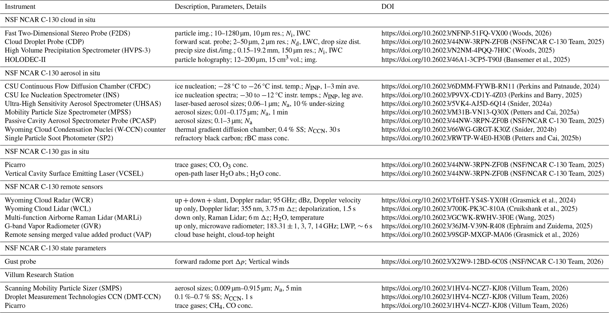
The RF02 flight track consisted of three surface legs (SL) flown at 300 m above sea level with spiral ascents/descents reaching 1750–2200 m in altitude bounding each SL (Fig. 1; the final ascent away from SL3 was in-line). Table S1 in the Supplement shows the sampling time as a function of altitude for each vertical profile. Each SL is approximately aligned with the southwest cold air advection, with SL1 and SL3 following approximately the same flow line. This allows SL1 and SL3 to be treated as a single interrupted SL, which we call SL13. SL2 lies beneath a different free tropospheric airmass than SL13, and is not the main focus of this analysis. Fetch distance along SL13 is defined as the distance downstream from the beginning of SL1. Distances are calculated following the flight path along SL1, across the gap between SL1 and SL3, and continuing along SL3. Table S2 provides a lookup table showing the time at various fetch distances. The instrumentation is summarized in Table A1, with a brief description provided below.

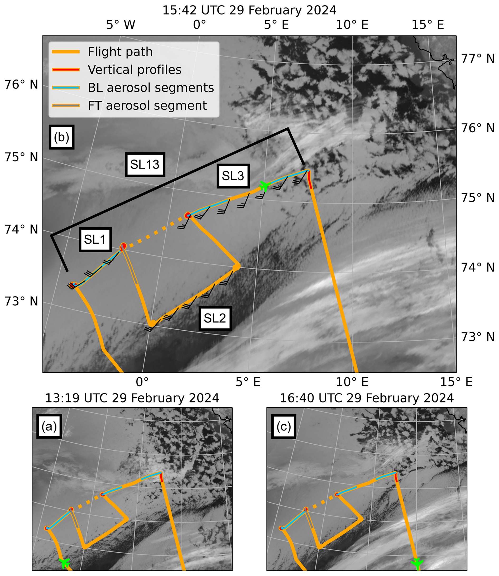
Figure 1 Infrared satellite imagery from the Advanced Very High Resolution Radiometer (AVHRR) at (a) 13:19 UTC, (b) 15:42 UTC, and (c) 16:40 UTC of the area of interest for RF02. In (b), the flight track (solid orange) and the connection of SL1 and SL3 (dashed orange) are labeled for each flight segment, and observed wind barbs (knots) are plotted at 5 min intervals when the plane is below 500 m altitude. Location and orientation of aircraft at time of satellite imagery is shown by the green airplane icon. Vertical profiles (red) are analyzed in Figs. 8, 9, 10, 11, and 12. Aerosol sampling segments in the BL (300 m; blue) and FT (1750 m; gray) are analyzed in Fig. 7. BL aerosol segments are also analyzed in Fig. C1.

2.1 In situ cloud

Only aircraft profiles depict the thermodynamic and microphysical vertical structure as no dropsondes were deployed along SL13. The Vertical Cavity Surface-Emitting Laser (VCSEL) hygrometer determines water vapor mixing ratios (WVMR), averaged to 1 Hz. A Cloud Droplet Probe (CDP, 2–50 µm diameter range) quantifies the liquid water content (LWC), cloud droplet concentration (N_d), and (liquid) drop size distribution (Lance et al., 2010). During profiles, the cloud-top height is determined by identifying the highest altitude with LWC >0.01 g m⁻³. The inversion level is defined as the altitude with the minimum temperature. Information on ice phase, ice water content (IWC) and N_i, is derived from two probes: the Fast 2-Dimensional Stereo Probe horizontal channel (F2DS, 10–1280 µm size range) and the High Volume Precipitation Spectrometer version 3 (HVPS-3, 150 µm–19.2 mm size range) (Lawson et al., 2006; Field et al., 2006). The F2DS and HVPS-3 size distributions are merged using a discriminating size threshold at 1000 µm. Particle phase is determined using a sphericity threshold of 0.7 (Korolev and Isaac, 2003) for particle sizes >100 µm. IWCs rely on the Brown and Francis (1995) mass-size parameterization. The Holographic Detector for Clouds v.2 (HOLODEC-II) provides additional information on particle habit (Spuler and Fugal, 2011). Given the HOLODEC-II's smaller sampling volume compared to the F2DS (0.015 versus 4.9 L at an aircraft speed of 100 m s⁻¹), any lack of drizzle drops within HOLODEC-II imagery is also checked against F2DS imagery at 10 µm pixel resolution. Particle Habit Imaging and Polar Scattering (PHIPS) data were not available for this flight.

2.2 Aerosol/gases

Refractory Black Carbon (rBC) mass concentrations, measured by a Single Particle Soot Photometer, (SP2, 70–900 nm scattering size range) indicate the presence of anthropogenic pollution (Cai et al., 2026). A merged aerosol number size distribution spanning 10 nm to 3 µm utilizes a Mobility Particle Size Spectrometer (MPSS, 0.01–0.175 µm), an Ultra-High Sensitivity Aerosol Spectrometer (UHSAS, 0.06–1 µm) and a Passive Cavity Aerosol Spectrometer Probe (PCASP, 0.1–3 µm), described in Cai et al. (2026). The size distribution is detailed for segments along SL13 and in the FT (shaded blue and gray respectively in Fig. 1) and provides the total aerosol number concentration (N_a). The Wyoming CCN Counter (W-CCN) provides N_CCN at a supersaturation of 0.4 % at 30 s resolution (Snider et al., 2006). N_CCN is only reported when LWC <0.01 g m⁻³ and IWC <0.1 g m⁻³. Both N_a and N_CCN are scaled to standard temperature and pressure (STP; 298.15 K, 1013.25 hPa) as in Cai et al. (2026). All aerosol and CCN data were collected in situ, by instrumentation inside the aircraft cabin and the wing-mounted PCASP cloud probe. N_INP is measured using both offline filter-based measurements processed on the Colorado State University (CSU) Ice Nucleation Spectrometer (INS; Hill et al., 2016; Barry et al., 2021) and online with the CSU Continuous Flow Diffusion Chamber (CFDC; Moore et al., 2024; Patnaude et al., 2025), both scaled to STP. INS measurements are averaged over longer sample times, but provide temperature spectra, whereas CFDC measurements provide higher time resolution at a single processing temperature, in this case from −28 to −26 °C. INS data from the offline filter samples collected over the course of the three surface legs (Fig. 2) are used to estimate N_INP at the approximate cloud-top temperature of −20 °C (N_INP20). A log-linear fit spans −29 to −20 °C, weighted by the uncertainty in measured points and constrained to pass through the data point at −20 °C. This fit multiplicatively corrects colder-temperature CFDC data to warmer temperatures. Error estimates on the corrected data apply lower and upper fit estimates to produce conservative CFDC 90 % confidence intervals. Ozone (O₃) and carbon monoxide (CO) concentrations measured by a Picarro gas analyzer help characterize entrainment (Appendix B).

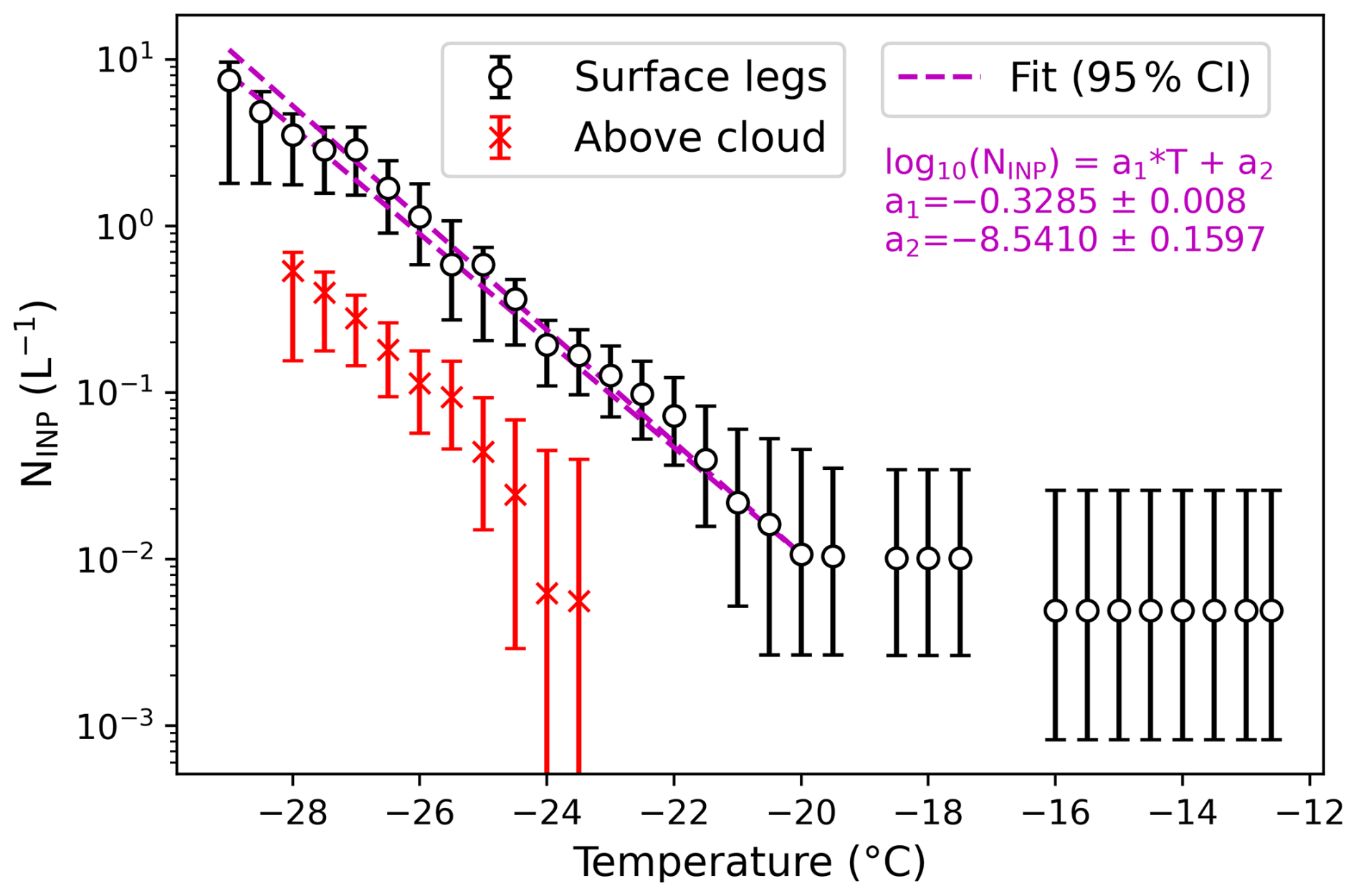
Figure 2 N_INP spectra measured by the INS during surface legs (black) and above cloud legs (red) with 90 % error bounds. The 95 % confidence interval of a log-linear fit of INS N_INP with respect to temperature during surface legs (magenta) corrects CFDC N_INP to the approximate cloud-top temperature of −20 °C.

2.3 Remote sensing

Surface legs allow the remote sensors to examine the cloud and sub-cloud structure. The 95 GHz Wyoming Cloud Radar (WCR) visualizes the cloud structure and its dynamics with radar reflectivities and Doppler velocities (Wang et al., 2012). Ice water path (IWP) is determined using a radar-estimated IWC $=\mathrm{0.10}\times Z^{\mathrm{0.51}}$ following Fuller et al. (2023), with attenuation not accounted for (Pokharel and Vali, 2011). A cloud top is identified when a radar echo of at least 75 m thick occurs below a non-echo (clear sky) region of at least 225 m thick. Cloud base height is determined through the gradient of the upward-viewing Wyoming Cloud Lidar (WCL) attenuated scattering ratio (Wang et al., 2012), at 1.5 m vertical resolution. The attenuated scattering ratio is the total attenuated backscatter divided by modeled attenuated molecular backscatter. The first attenuated scattering ratio gradient exceeding an empirically-derived threshold becomes the WCL-estimated cloud base. LWPs are retrieved using upward-pointing G-band Vapor Radiometer (GVR) brightness temperatures combined with WCR reflectivities (Ephraim et al., 2025).

The downward-pointing Multi-function Airborne Raman Lidar (MARLi), in its first C-130 deployment, retrieves vertical profiles of WVMR and temperature at 0.6 Hz temporal resolution (∼150 m at a 100 m s⁻¹ aircraft speed) with a vertical resolution of 6 m (Liu et al., 2014; Wu et al., 2016). Retrievals are excluded within 100 m of the aircraft due to an uncertain near-range overlap correction. The hydrostatic relation in combination with in situ flight-level pressure further provides below-aircraft vertical profiles of pressure. Virtual and equivalent potential temperature (θ_v and θ_e) profiles, based on the WVMR, temperature, and pressure profiles, identify cold pools and entrainment events. MARLi-derived θ_v and θ_e are shifted by a small constant offset (+2.1 K for SL1; +1.0 K for SL3) to bring consistency across the 100 m gap between flight level and the highest valid MARLi level. Cold pools are defined by local θ_v minima, at 60 m altitude, of at least 0.5 K lower than adjacent values, with the maximum difference (Δθ_v) defining the intensity and cold pool width (the distance over which Δθ_v is $\le -\mathrm{0.5}$ K). Potential entrainment events are defined by a 60 m altitude WVMR at least 0.25 g kg⁻¹ drier than the leg-specific linearly-detrended WVMR (ΔWVMR), used to define intensity, and collocated with a similarly-defined positive 60 m altitude θ_v anomaly.

2.4 Models, reanalyses and satellite data

The ECMWF Reanalysis V5 (ERA5; Hersbach et al., 2020) reconstructs the large-scale mean sea level pressure (MSLP) field, and determines the sea ice edge and MCAO conditions, at 0.25° resolution. More intense MCAO conditions are more unstable, determined through the M-index: θ_skinSST−θ_850 hPa (Papritz et al., 2015). The M-index is not calculated where ERA5 sea ice concentrations exceed 15 %, defined as the sea ice edge. Archived initializations of AROME-Arctic, a convection-allowing 2.5 km spatial resolution model developed by the Norwegian Meteorological Institute, serve as a high-resolution reanalysis (Müller et al., 2017). Thermal infrared imagery from the NOAA-20 VIIRS, MetOp-B AVHRR, and NOAA-19 AVHRR visualizes the cloud field. The surface wind field near the end of SL3 is retrieved by the Synthetic Aperture Radar (SAR) aboard RadarSat Constellation Mission-1 (RCM-1).

2.5 Back-trajectories and Villum Research Station

Footprint emission sensitivities calculated by the FLEXable PARTicle dispersion model (FLEXPART), a Lagrangian transport and dispersion model (Pisso et al., 2019), indicate that air sampled during SL13 passed near the Villum Research Station at Station Nord (81°36^′ N, 16°40^′ W), located in northeast Greenland. Back-trajectories calculated using the HYbrid Single Particle Lagrangian Integrated Trajectory (HYSPLIT) model, initialized using ERA5, further confirm this. Data from Villum Research Station thus establishes aerosol conditions upwind of SL13. At Villum, a Scanning Mobility Particle Sizer (SMPS, 9 nm to 0.915 µm size range) provides the aerosol number size distribution, and a Droplet Measurement Technologies CCN counter (DMT-CCN) provides N_CCN at discrete supersaturations between 0.1 % and 0.7 %. Both N_a and N_CCN are scaled to STP (298.15 K, 1013.25 hPa) as in Cai et al. (2026). A Picarro Cavity Ringdown Spectrometer provides methane (CH₄) and CO concentrations.

3 Synoptic overview

On 26 February 2024, a sharp shortwave trough is situated southeast of Greenland, with a large area of diffluent flow over Iceland and the surrounding waters (not shown). A remnant surface low situated just west of Iceland rapidly strengthens underneath the large-scale divergence aloft, further enhanced by upward motion in the left exit region of the jet streak (not shown). Both the trough and surface low propagate towards the east-northeast. By 12:00 UTC on 27 February 2024, the trough becomes cutoff and vertically stacked with the surface low around 200 km northeast of Iceland, limiting upper level support. Research flight RF01 on 28 February and RF02 on 29 February sampled different portions of this surface low's MCAO sector.

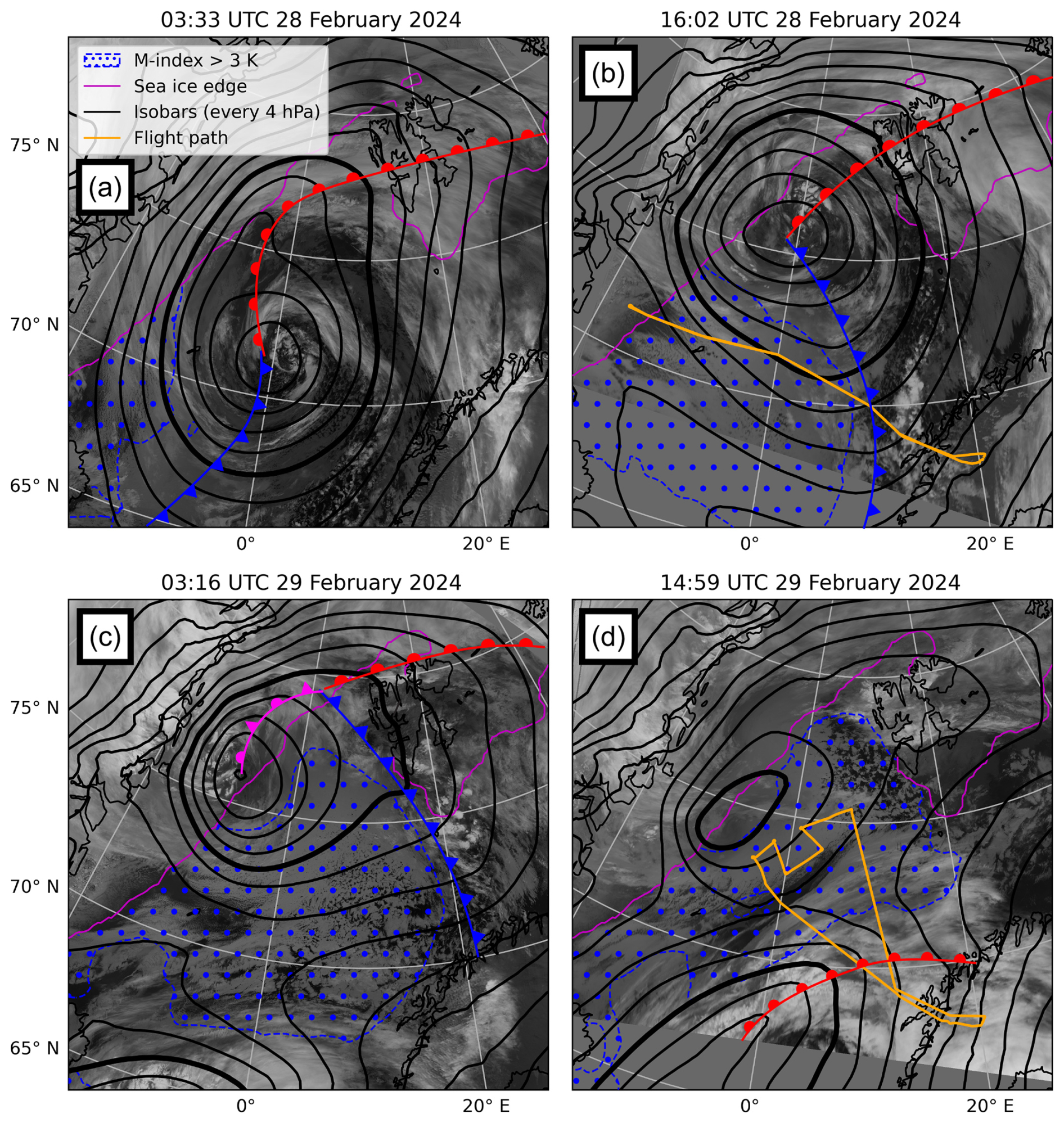
Figure 3 Infrared satellite imagery overlaid with ERA5 MSLP contours every 4 hPa (980 hPa bolded), surface fronts, M-index >3 K (blue hatches), and the ERA5 sea ice edge (magenta line) at 28 February 2024 (a) 03:33 UTC, (b) 16:02 UTC, with the RF01 flight track indicated; 29 February 2024 (c) 03:16 UTC, and (d) 14:59 UTC with the RF02 flight track indicated.

By 03:00 UTC on 28 February, the low has moved northward (Fig. 3a). Despite lacking upper-level support, the low is still situated along a strong baroclinic zone, maintaining a maximum strength of approximately 960 hPa. A warm frontal zone stretches across Svalbard and cloud cover from a warm air intrusion spans from northern Scandinavia towards Svalbard. MCAO conditions are limited to the area between the island of Jan Mayen (70°59^′ N, 8°32^′ W) and Iceland behind a cold front with cold air advection off the sea ice supporting cloud streets.

By 16:00 UTC on 28 February, the low has moved to the north while maintaining its minimum central pressure (Fig. 3b). Strong low-level cold air advection off of the Greenland marginal ice zone creates a broad region of MCAO conditions. The cold front bounding this air mass contains a line of convection just off the Norwegian coast stretching towards Svalbard. RF01 sampled the post-frontal MCAO clouds, but this air mass moved north of the region sampled 1 d later during RF02.

By 03:00 UTC on 29 February, the center of the low is encircled by the MCAO, completing the occlusion process and causing the low to rapidly weaken (Fig. 3c). MCAO conditions stretch nearly all the way from the sea ice edge off eastern Greenland to the Norwegian coast, with a closed-to-open cell cloud transition occurring at around 5° E. The strong pressure gradient between the surface low and Greenland constrains the air flowing south past Villum to remain over the marginal ice zone. A new synoptic low (centered near 62° N, 10° W) further south encroaches, with warm air advection bounding the southern edge of the MCAO region. Twelve hours later, by 15:00 UTC, the occluded surface low driving the MCAO has weakened by 16 hPa (Fig. 3d). Warm air advection from the southern synoptic low reduces the southern extent of the MCAO and supports a cloud shield, also sampled by the remote sensors during the ferry legs of RF02 at 6 km altitude (Zuidema et al., 2026). The lower-level RF02 sampling took place within the MCAO persisting to the north of the encroaching warm air intrusion (orange track in Fig. 3d).

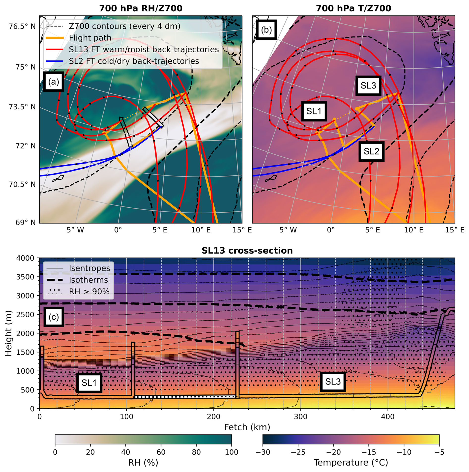
Figure 4 AROME-Arctic 15:00 UTC model run analysis field (0 h forecast). (a) 700 hPa RH (shaded), geopotential height (dashed contours every 4 dm; 264 dm bolded), SL1 and SL3 flight tracks (solid orange, connected using a dashed orange line). Back-trajectories terminating at 2500 m along SL13 (red) and SL2 (blue), with black dots every 3 h. In situ RH for two legs flown at altitudes of 1700–2100 m, within black outlines. (b) 700 hPa temperature (shaded) with same geopotential height contours and back-trajectories as in (a) and SL1, SL2, SL3 legs labeled. (c) Cross-section along SL13 of air temperature (shaded) with −15, −20, and −25 °C above-inversion temperatures indicated (thick dashed contours). Potential temperature also indicated (thin solid contours every 1 K), and RH >90 % (hatched). In situ air temperature and potential temperature indicated inside black outlines (including spiral profiles).

Despite the close proximity of SL13 to SL2, AROME-Arctic depicts different capping free tropospheric conditions (Fig. 4a, b). The 700 hPa air above most of SL13 at 15:00 UTC is moist, with relative humidities (RH) >90 %, compared to RH <10 % over SL2 (Fig. 4a). In situ FT measurements made during the cross legs from SL1 to SL2 and SL2 to SL3 confirm the sharp horizontal RH gradients in AROME-Arctic (Fig. 4a). During the cross leg from SL2 to SL3 flown at 2050 m, just 27 km south of the spiral descent to SL3, WVMR increases from 0.05 to 1.25 g kg⁻¹ over 9 km. The 700 hPa temperature at 09:00 UTC was also warmer above SL13 ($>-\mathrm{18}$ °C versus $<-\mathrm{20}$ °C above SL2; not shown), prior to becoming modified by warm air advection (Fig. 4b). This is because more of the FT air above SL13 originates from the mid-latitudes (red back-trajectories in Fig. 4a, b) before wrapping around the occluded low. In contrast, SL2 resides below a modified cold, dry FT air mass originating from Greenland (blue back-trajectories in Fig. 4a, b). The air mass boundary is also apparent in in situ FT gas concentrations measured during both cross legs, with O₃ decreasing from 134 to 51 ppbv and CO increasing from 81 to 115 ppbv between SL2 to SL3 (not shown). The two airmasses do become linked closer to Svalbard, where the cold airmass above SL2 forms a lobe of cold air located southwest of Svalbard (Fig. 4b). This creates a horizontal FT temperature gradient at the end of SL13 that ultimately weakens the cloud-top inversion (Fig. 4c).

A vertical AROME-Arctic cross section along SL13 (Fig. 4c) depicts the gradual deepening of the boundary layer (BL), driven by modeled buoyancy fluxes averaging 260 W m⁻² during SL1 (sensible/latent heat fluxes of 260/140 W m⁻²), decreasing to 200 W m⁻² during SL3 (sensible/latent heat fluxes of 190/140 W m⁻²) (not shown). The 700 hPa temperatures decrease by approximately 3 K along SL13, evident in the downward slope of isotherms. The cooling reduces the inversion strength, evident in the increased spacing of isentropes (thin solid lines) with fetch. The FT RH increases with fetch (dotted regions in Fig. 4c), consistent with observed mid-level clouds (Fig. 1). In situ profiles (discussed in Sect. 5) confirm the gradient in the AROME-Arctic FT thermodynamic values, although the inversion is both ∼400 m lower and less sharp in AROME-Arctic compared to our observations (Fig. 4c).

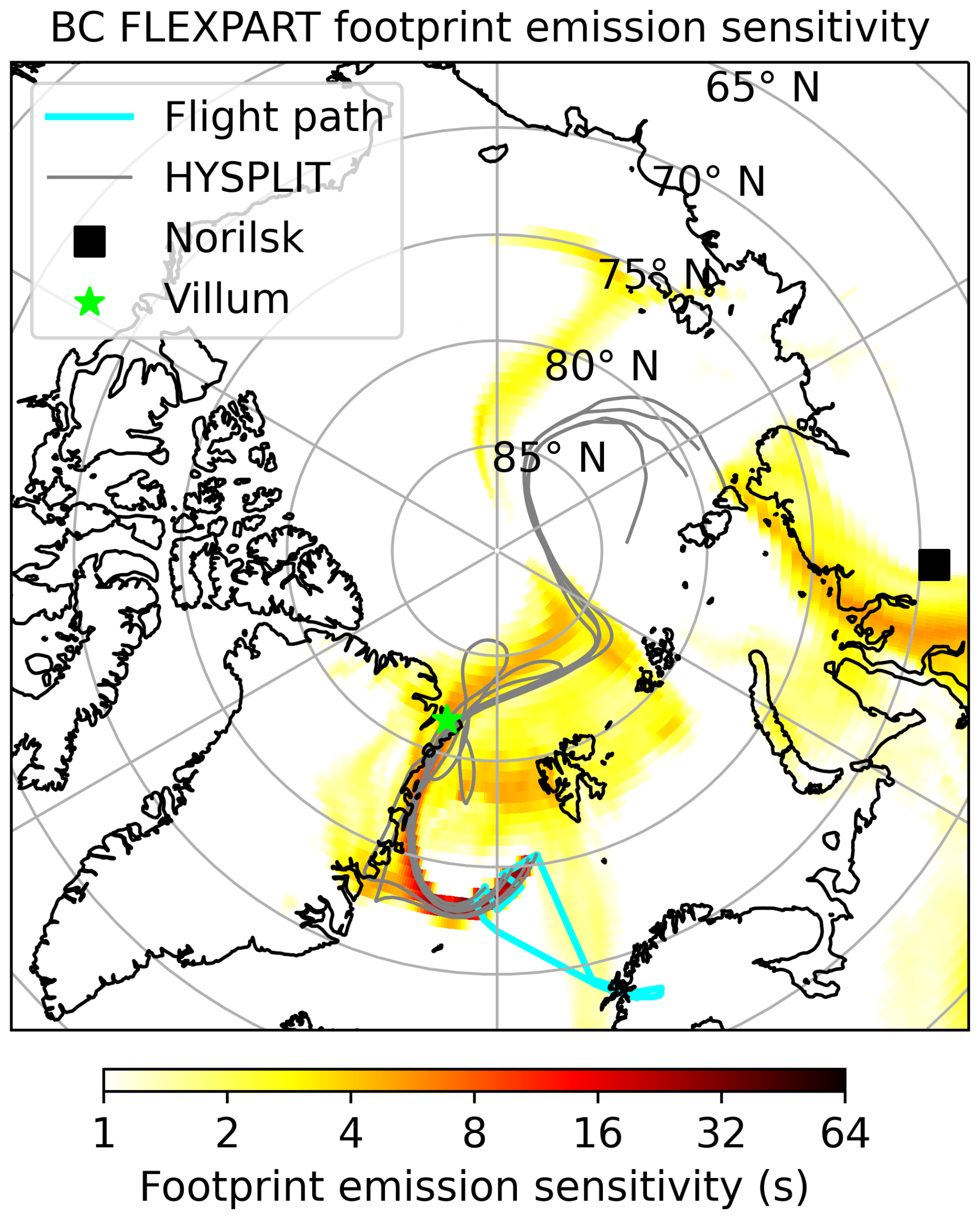
Figure 5 Black carbon FLEXPART footprint emission sensitivities for receptor points at flight level along SL1 and SL3 (yellow shading). HYSPLIT back-trajectories with receptor points at 500 m are overlaid (gray lines) on the RF02 flight path (turquoise line).

4 The relationship of CAESAR aerosol measurements to those upwind at Villum

CCN concentrations during SL1 were the highest observed during CAESAR, occasionally surpassing 800 cm⁻³. HYSPLIT back-trajectories and a FLEXPART footprint analysis of BC, initialized within the SL13 boundary layer (Fig. 5), indicate the airmass likely originated from near Norilsk, Russia. Norilsk hosts the world's largest producer of Nickel and also smelts other metals, making Norilsk one of the world's largest SO₂ emission hotspots (Bauduin et al., 2014; Nilsen, 2019) and Russia's most polluted city (Lyrchikova, 2023). GEOS-CF simulations (Fig. S1 in the Supplement) further corroborate the back-trajectories, by indicating a buildup of SO₂ originating from Russia over the central Arctic 2 d before RF02. In the day prior to RF02, a filament advects along the east coast of Greenland before deflecting around the occluded low and into RF02's flight domain.

Back-trajectories initialized along SL1 and SL3 pass within 60 km of Villum Research Station on 01:00–02:00 UTC, 29 February, approximately 13 h prior, and 01:00–22:00 UTC, 28 February, approximately 17–31 h prior, respectively (Fig. 6). The longer travel times for the SL3 back-trajectories reflect the weaker winds near the center of the low, compared to the winds encountered by the SL1 air mass.

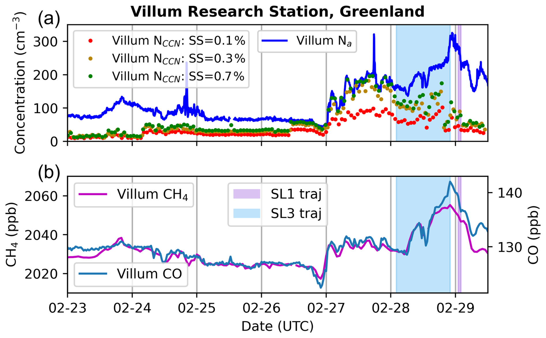
Figure 6 Observations taken from the Villum Research Station at Station Nord, Greenland consisting of: (a) Aerosol and CCN concentrations. (b) CH₄ and CO volume mixing ratios. Back-trajectories from SL1 pass Villum from 01:00–02:00 UTC, 29 February (lilac shading) and from SL3 on 01:00–22:00 UTC, 28 February (light blue shading), respectively.

N_a, CH₄, and CO first increase at Villum on 27 February, and continue to increase to 326 cm⁻³, 2054 ppbv, and 142 ppbv respectively until 00:00 UTC, 29 February, before decreasing again (Fig. 6). The correlation coefficients between N_a and ${\mathrm{CH}}_{\mathrm{4}}/\mathrm{CO}$ are 0.84/0.87, respectively, consistent with an anthropogenic origin. A decrease in N_CCN at a 0.3 % supersaturation from 150 to 41 cm⁻³ from 21:00 UTC, 28 February, to 00:00 UTC, 29 February, coincides with an increase in N_a, suggesting the CO and CH₄-enriched air mass also contains less hygroscopic aerosol (Fig. 6a).

The mean aerosol number size distribution at Villum corresponding to the SL1 back-trajectories has a dominant accumulation mode with a peak diameter near 110 nm (Fig. 7), similar to central springtime Arctic observations (Boyer et al., 2023). A small enhancement in aerosol concentrations from 10–30 nm (Fig. 7) is potentially indicative of new particle formation. The mean aerosol number size distribution at Villum corresponding to the SL3 back-trajectories is unimodal with an accumulation mode peak near 110 nm (Fig. 7). The time-mean N_a corresponding to the SL1 back-trajectories at Villum of 266 cm⁻³ exceeds that of 194 cm⁻³ corresponding to the SL3 back-trajectories.

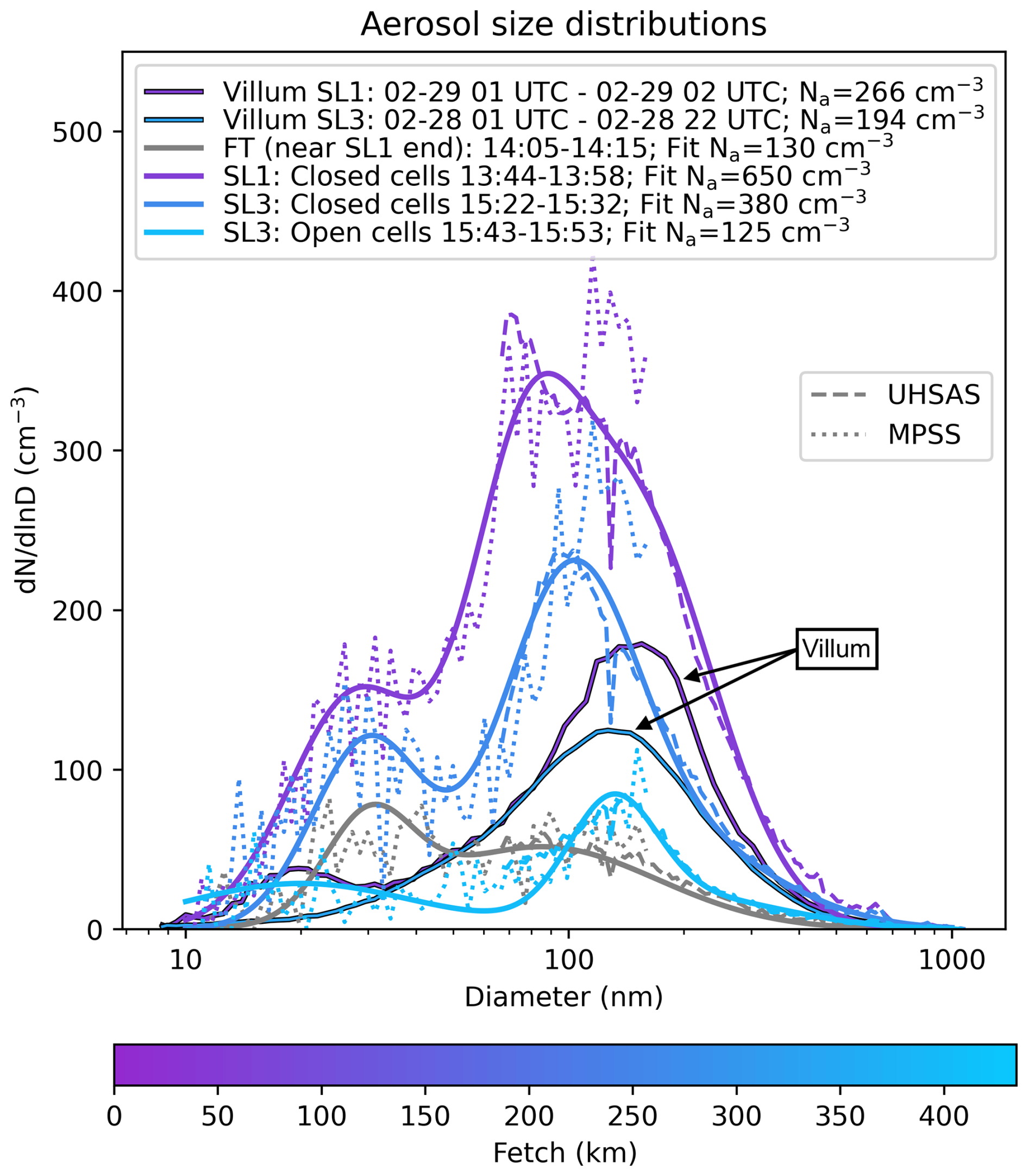
Figure 7 Mean aerosol number size distributions at Villum corresponding to back-trajectories from SL1 and SL3 (shading in Fig. 6), for three flight segments along SL13 (300 m; blue in Fig. 1), and one flight segment in the FT (1750 m; gray in Fig. 1). The Villum aerosol number size distribution is based on SMPS measurements only. The SL1, SL3, and FT aerosol size distributions are a fit based on a merging of UHSAS, MPSS and PCASP (not shown) aerosol number size distributions (Cai et al., 2026). Size-integrated total number concentrations (N_a) indicated in legend.

Overall N_a values are less at Villum than during RF02 (Fig. 7). By the beginning of SL1, 4 h after the air mass has left the sea ice edge and 13 h after flowing past Villum, the aerosol number size distribution is bimodal, with a larger primary accumulation mode centered at 100 nm, and an additional smaller secondary Aitken mode centered at 20–40 nm, separated by a minimum at 40–50 nm (Fig. 7). The Aitken and accumulation mode aerosol number concentrations (N_ait and N_acc) exceed those measured on Svalbard in MCAO conditions (Williams et al., 2024). Observed (collocated) N_a/N_CCN decrease from 650/680 cm⁻³ during SL1, to 380/350 cm⁻³ at the beginning of SL3, to 125/90 cm⁻³ by the end of SL3 (Fig. 7). N_CCN is sometimes higher than N_a, attributed to instrument uncertainty. BL CO concentrations of 140–150 ppbv measured during vertical profiles are consistent with values measured at Villum between 21:00 UTC, 28 February, and 01:00 UTC, 29 February (Figs. 6b, 8a–c). This suggests new aerosol sources, such as from sea spray production during transit over open water can help explain the N_a increase. Sampling differences between the two locations (surface observations in a vertically stratified environment at Villum vs. airborne observations in a mixed BL during RF02) may also contribute.

By the time the air is sampled during RF02, CO and O₃ are both well-mixed within the SL1 BL profiles (Fig. 8a–c), underneath a FT with more O₃ and less CO. The FT gas concentrations remain relatively constant during SL1. Some rBC is also present in the boundary layer, consistent with an anthropogenic origin. By the last vertical profile, both the BL rBC and N_CCN have declined substantially. The last ascent, at the end of SL3, is into a distinct FT airmass with higher O₃ concentrations and lower CO concentrations as the aircraft turned towards the south (Figs. 1, 8d).

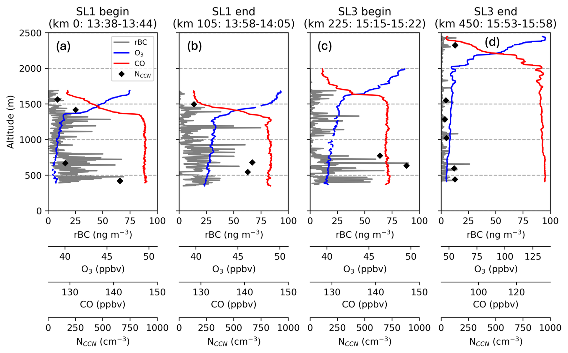
Figure 8 Profiles of rBC, O₃, CO, and N_CCN from the (a) spiral descent into SL1 from 13:38–13:44 UTC, (b) spiral ascent out of SL1 from 13:58–14:05 UTC, (c) spiral descent into SL3 from 15:15–15:22 UTC, and (d) in-line ascent out of SL3 from 15:53–15:58 UTC, all on 29 February, at locations depicted in Fig. 1. Note the different scale of O₃ and CO in (d).

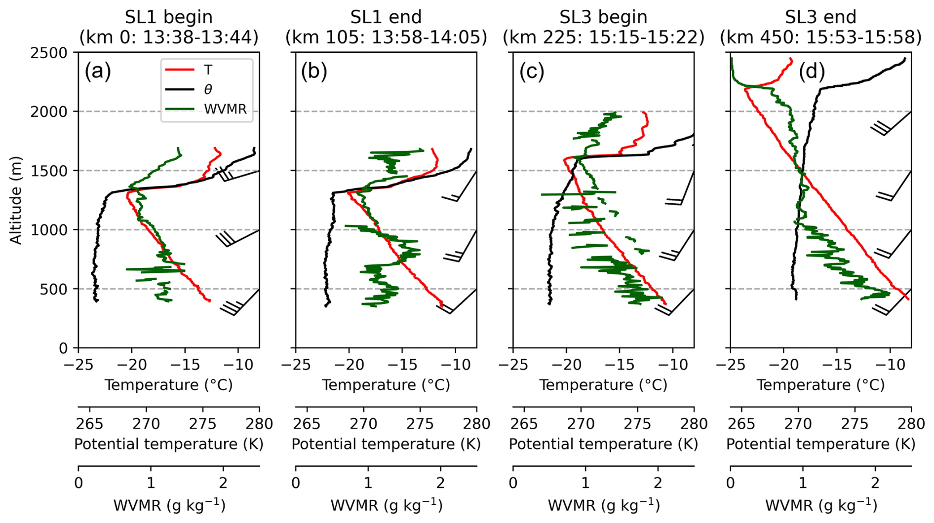
Figure 9 Thermodynamic profiles conducted during (a) spiral descent into SL1 from 13:38–13:44 UTC, (b) spiral ascent out of SL1 from 13:58–14:05 UTC, (c) spiral descent into SL3 from 15:15–15:22 UTC, and (d) in-line ascent out of SL3 from 15:53–15:58 UTC, all on 29 February, at locations depicted in Fig. 1. Profiles are of temperature (red line), potential temperature (black line) and WVMR (dark green line) with wind barbs (knots) at 500 m intervals. WVMR values decrease due to icing on the VCSEL at times, notably in panel (c).

5 Thermodynamic and microphysical profiles indicate the boundary layer remains well-mixed with distance

The four vertical profiles bounding SL1 and SL3 straddle 450 km (Fig. 1), with the first three profiles done as spirals to minimize spatial variability. Over this distance, BL heights increase from 1270 to 2180 m, sub-cloud BL potential temperatures (θ) increase from 265 to 270 K, and flight-level temperature/moisture increases and moistens from −13 °C/1.2 g kg⁻¹ to −8 °C/2 g kg⁻¹ (Fig. 9). Sub-cloud θ profiles indicate the BL is well-mixed (as do CO and O₃ in Fig. 8), while southwesterly BL winds of 12–17 m s⁻¹ gradually weaken with fetch (Fig. 9). The boundary layer is capped by a strong ∼ 10 K temperature inversion (Fig. 9a–c), with more water vapor in the FT than within the BL in all three spiral profiles (Fig. 9a–c). During the rapid in-line ascent from SL3 through open-cell convection, the aircraft traveled southward (Fig. 1) and ascended into a much drier FT airmass, consistent with crossing the sharp gradient in FT moisture shown in AROME-Arctic (Figs. 4a, 9d).

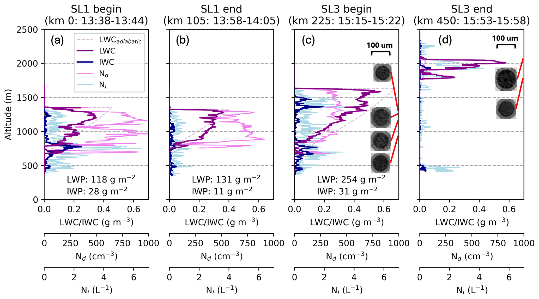
Figure 10 Microphysical profiles conducted during (a) spiral descent into SL1 from 13:38–13:44 UTC, (b) spiral ascent out of SL1 from 13:58–14:05 UTC, (c) spiral descent into SL3 from 15:15–15:22 UTC, and (d) in-line ascent out of SL3 from 15:53–15:58 UTC, all on 29 February, at locations depicted in Fig. 1. Profiles include LWC (thick dark magenta line), IWC (thick dark blue line), N_d (thin pink line), and N_i (thin light blue line). Adiabatic LWC is calculated between cloud base (lowest altitude LWC >0.01 g m⁻³) and cloud top (highest altitude LWC >0.01 g m⁻³) in (a)–(c). HOLODEC-II images of drizzle larger than 75 µm are shown. LWP (IWP) are integrated using in situ LWC (IWC).

The profiles bounding SL1 sampled liquid-dominated clouds with approximately adiabatic LWC profiles, corresponding to LWPs of 118 and 131 g m⁻² (Fig. 10a, b). LWCs surpass 0.3 g m⁻³ at temperatures below −20 °C with cloud tops, reaching 1310–1320 m, overshooting the inversion by 10–40 m (Fig. 10a, b). N_d exceeds 600 cm⁻³ in both profiles bounding SL1 (Figs. 10a, b, 11). An N_a–N_d closure (Appendix C) using an adiabatic cloud parcel model (Rothenberg and Wang, 2016) establishes confidence in the unusually high N_d observations. Nearly all drops are <15 µm, and 80 % of all drops are <10 µm at both the beginning and end of SL1 (Fig. 11). No drizzle (>75 µm) is observed by HOLODEC-II in either profile, although at least one drizzle drop was captured by the larger sampling volume of the F2DS during both profiles (not shown). The effective diameters within 100 m of cloud top at the beginning and end of SL1 are 11.6 and 8.5 µm respectively (not shown). HVPS-3 microphysical imagery indicates dendrites, aggregates, and small rimed ice throughout the cloud (Fig. 12a, b). The growth of dendrites and aggregates through vapor deposition is favored given cloud temperatures of −20 to −15 °C in the presence of small supercooled droplets. N_i remains below 3 L⁻¹, with the exception of a spike to 6.5 L⁻¹ at 750 m during the descent to SL1 (Fig. 10a).

By the spiral descent to SL3, the average in-cloud N_d has decreased to 302 cm⁻³ (Figs. 10c, 11), with a sharply adiabatically-distributed supercooled LWC reaching a maximum of 0.58 g m⁻³ at the inversion height, corresponding to a LWP of 254 g m⁻². The cloud-top height overshoots the inversion height by 20 m. The drop size distribution has shifted to larger sizes, with 60 % of drop diameters >10 µm (Fig. 11), and an effective diameter within 100 m of cloud top of 16.1 µm (not shown). Drizzle (>75 µm) is observed by the HOLODEC-II between 880 m (−15.5 °C) and 1290 m (−18.6 °C) (Fig. 10c). Riming becomes more obvious, with rimed particles larger and more numerous (Fig. 12c). N_i remains <3 L⁻¹ (Fig. 10c), however.

The rapid in-line ascent from SL3 through open-cell convection passes through clear sky prior to clipping the top of a convective cell (indicated in WCR reflectivity; not shown) with two discrete peaks of LWC: 0.23 g m⁻³ at 1790 m and 0.58 g m⁻³ at 2010 m (Fig. 10d). Average in-cloud N_d is now reduced to 32 cm⁻³, consistent with larger drop sizes: 80 % of drops have diameters between 20 and 30 µm (Fig. 11), and drizzle (>75 µm) is observed by HOLODEC-II at temperatures as low as −22 °C (Fig. 10d). Large graupel are present, with diameters reaching 5 mm (Fig. 12d).

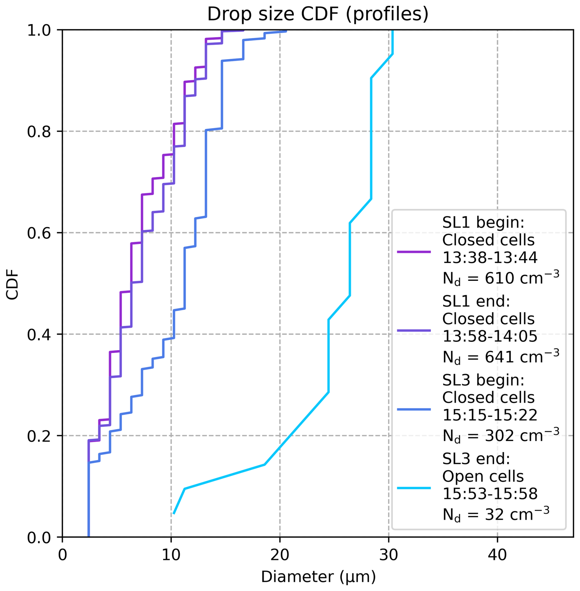
Figure 11 Cumulative distribution function (CDF) of the drop size distributions for each vertical profile in Fig. 10. Drop size distributions and profile-mean N_d (in legend) only include areas between the highest and lowest observation of LWC >0.05 g m⁻³ in each profile. Line color indicates fetch using the color scale in Fig. 7.

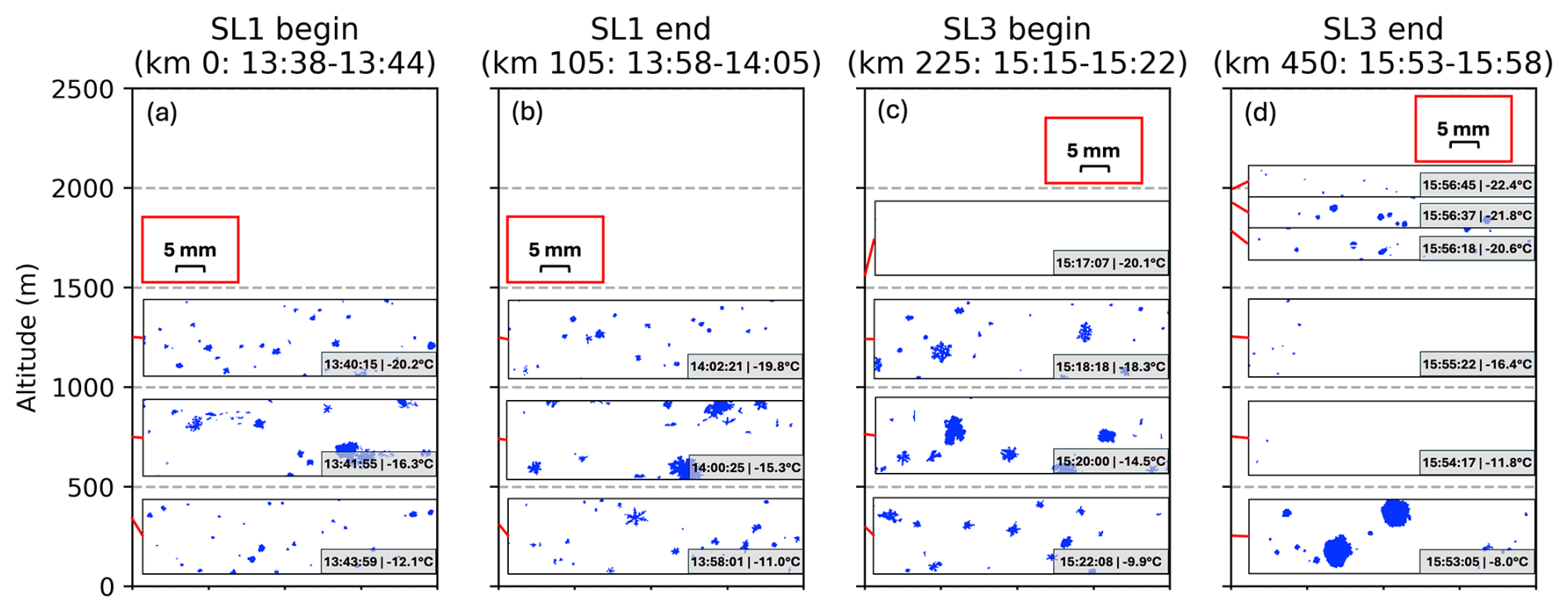
Figure 12 HVPS-3 microphysical imagery profiles conducted during (a) spiral descent into SL1 from 13:38–13:44 UTC, (b) spiral ascent out of SL1 from 13:58–14:05 UTC, (c) spiral descent into SL3 from 15:15–15:22 UTC, and (d) in-line ascent out of SL3 from 15:53–15:58 UTC, all on 29 February, at locations depicted in Fig. 1. The altitude of each image is indicated (red line), with the time and ambient air temperature noted in the bottom right of each image. Scale provided near top in the red boxes, repeated for convenience.

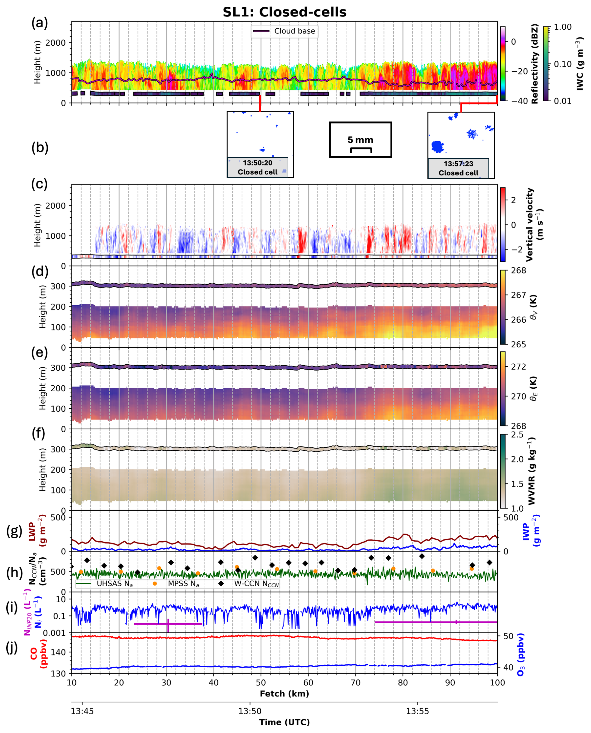
Figure 13 Observations during SL1 (13:44–13:58 UTC). In situ observations indicated at flight level (300 m) inside a black outline. (a) WCR reflectivity with lidar-derived cloud base (magenta line) and in situ IWC; (b) Two HVPS-3 images, at 13:50:20 and 13:57:23 UTC; (c) WCR Doppler velocity (1 m s⁻¹ added to offset fall speed of hydrometeors) and in situ vertical velocity; (d) MARLi-derived and in situ θ_v; (e) MARLi-derived and in situ θ_e; (f) MARLi and in situ WVMR (g kg⁻¹); (g) GVR-retrieved LWP (g m⁻², brown line) and radar-retrieved IWP (g m⁻², blue line); (h) W-CCN N_CCN (black diamonds) and UHSAS/MPSS N_a (dark green line and orange filled circles, respectively); (i) In situ N_i (L⁻¹, blue line) and CFDC derived N_INP20 (L⁻¹, magenta cross indicating sample duration and error bounds); (j) Picarro O₃ and CO concentrations (ppbv, blue and red lines respectively).

Figure 14 Same as Fig. 13 but for SL3 (15:22–15:53 UTC). The scale for θ_v and θ_e in (d) and (e) are shifted up from those in Fig. 13. Locations where cold pools (entrainment) are identified are underlined in blue (gold) in (d)–(f).

6 Boundary layer evolution along SL13

6.1 Closed-cell boundary layer warms and moistens during SL1

Closed-cell convection throughout SL1 reaches cloud-top heights averaging 1230±90 m over the 12 min 90 km leg (Fig. 13a). Updraft velocities occasionally surpass 3 m s⁻¹ (Fig. 13c), more apparent later in the leg. The BL warms and moistens throughout, evident in the below flight-level MARLi-derived θ_v, θ_e, and WVMR profiles (Fig. 13d, e, f). Cloud bases average 660 m, slightly decreasing towards the end of the leg, consistent with the increasing sub-cloud WVMR (Fig. 13a, f). LWPs increase throughout SL1, from 120 g m⁻² (km 10 to km 40) to 180 g m⁻² (km 70 to km 100) (Fig. 13g) with N_CCN concentrations occasionally surpassing 800 cm⁻³ (Fig. 13h). The supercooled liquid supports the in-cloud growth of ice particles, detected as small rimed particles, dendrites, and aggregates at flight level (Fig. 13b). Liquid-equivalent precipitation rates remain less than 0.5 mm h⁻¹ (flight-level IWC <0.14 g m⁻³) assuming a fall speed of 1 m s⁻¹, too light to generate obvious cold pools. No drizzle is evident in HOLODEC-II imagery at flight level (not shown). The 75th percentile of N_i during SL1 is 1.0 L⁻¹ with a maximum of 4.9 L⁻¹ at km 91, 50–500× higher than N_INP20, consistent with SIP (Fig. 13i, Table 1).

Table 1 N_INP as measured by the CFDC along segments of SL13. CFDC processing temperature and N_INP20 for each leg is also included. 90 % confidence interval is indicated. Any concentration below the CFDC limit of detection is reported as zero.

6.2 Cold pools and entrainment are hypothesized to help organize the closed-to-open cell transition

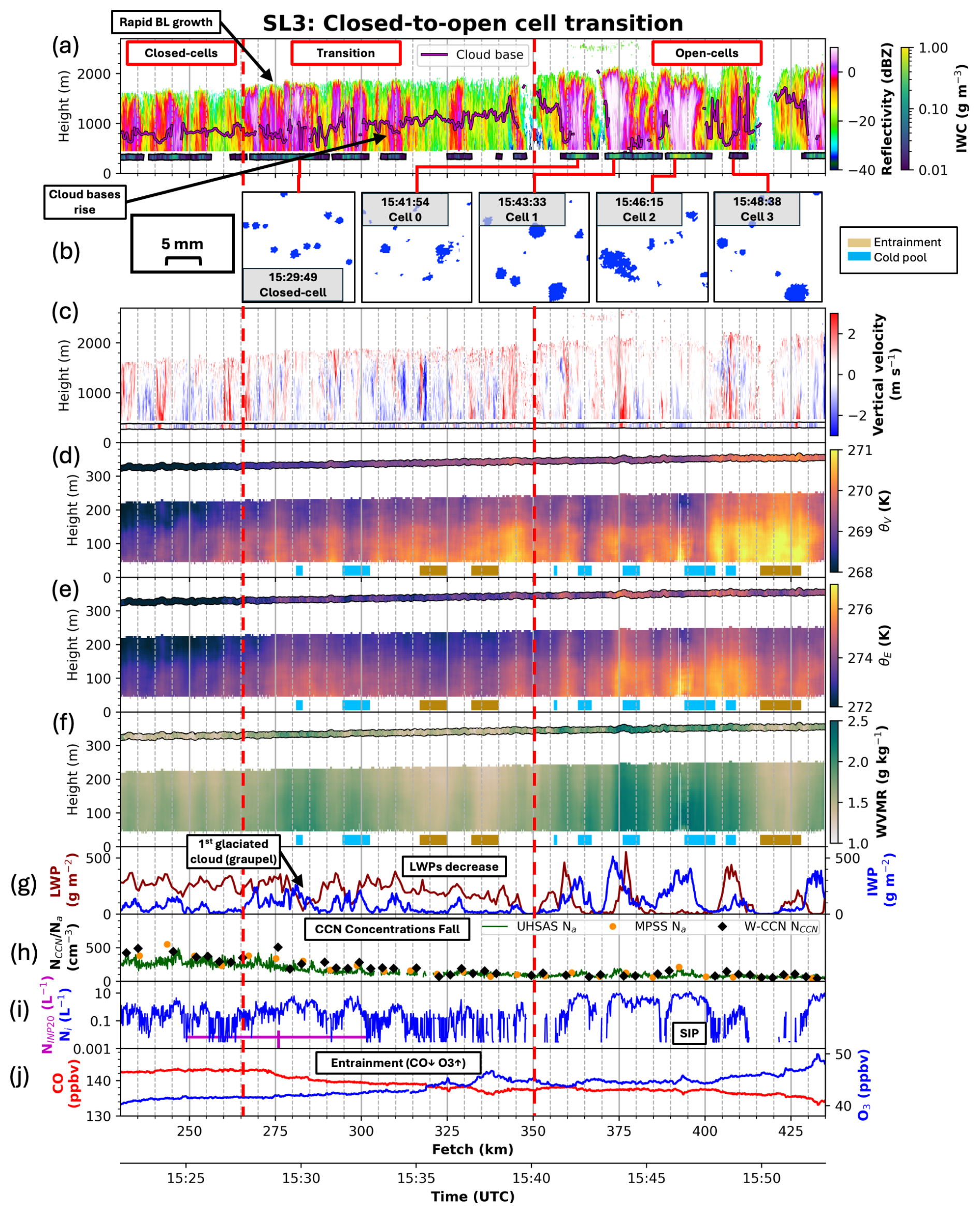
Remote sensing and in situ observations, analogous to those for SL1 in Fig. 13, indicate SL3 can be divided into three stages (Fig. 14): closed-cells (km 230 to km 265), transition (km 265 to km 350), and open-cells (km 350 to km 435). Precipitation along SL3 is all ice, with no drizzle evident in HOLODEC-II imagery (not shown).

The closed-cells at the beginning of SL3 possess LWPs of 270±50 g m⁻² and average cloud-top heights of 1520 m, an increase of 290 m since SL1 (Fig. 14a, g). Flight-level IWC reaches a maximum of 0.25 g m⁻³ at km 247 (Fig. 14a) with a 75th percentile (maximum) N_i of 0.62 L⁻¹ (4.5 L⁻¹) – 90–700× higher than N_INP20 (now decreased to 0.0067 L⁻¹ compared to SL1) (Fig. 14i, Table 1). The average N_CCN has decreased from SL1, to 390 cm⁻³ (Fig. 14h).

The first hint of a transition to open-cell convection appears when cloud tops increase rapidly from 1540 to 1760 m between km 265 and km 285 (Fig. 14a). Simultaneously BL CO rapidly drops while O₃ increases (Fig. 14j). All three observations indicate entrainment. The first mostly glaciated cloud is observed at km 282, with a radar-derived IWP reaching 260 g m⁻² and a decrease in LWP from approximately 300 to 50 g m⁻² (Fig. 14a, g). Small graupel (diameters of 1 mm) reaches flight level (Fig. 14b) with IWC reaching 0.24 g m⁻³ and N_i reaching 6.3 L⁻¹ (Fig. 14a, i). The precipitation shaft near km 282 generates the first observed cold pool (Δθ_v of −0.6 K; width of 2 km) (Fig. 14d). A cold pool is also present centered at km 297 (Δθ_v of −0.8 K; width of 8 km), similarly associated with ice precipitation falling from a mostly glaciated cloud (Fig. 14a, d, g). 25 km further downstream, warm θ_v anomalies (Fig. 14d), dry WVMR anomalies (Fig. 14f), and a suppressed reflectivity structure (Fig. 14a), indicate the first entrainment event reaching within 60 m of the ocean surface, centered at km 322 (ΔWVMR of −0.3 g kg⁻¹; width of 8 km), followed by another at km 337 (ΔWVMR of −0.4 g kg⁻¹; width of 8 km). Nearby these events, O₃ (CO) increases (decreases) at km 319 and km 335 (Fig. 14j). The drying of the BL is associated with decreasing LWP and IWP (Fig. 14g), with the first clearing observed at km 350 (Fig. 14a). Cloud bases rise from 640 m at the beginning of SL3 to 1070 m averaged from km 315 to km 350 (Fig. 14a). Cross-track advection of air, previously dried through entrainment with the dry FT airmass to the south of SL3, may also contribute to drying the BL and rising (falling) O₃ (CO) concentrations (Fig. 4a). We note any sublimation/evaporation of precipitation into a drier BL will decrease temperature more than if sublimating into a moist BL, further aiding the formation of cold pools. N_CCN decreases from 390 cm⁻³ during the closed-cell segment to 135 cm⁻³ by the end of the transition segment (km 325 to km 350; Fig. 14h).

6.3 Cold pools do not decouple the boundary layer during open-cell convection

Within open-cells, frozen precipitation reaches flight level with in situ IWCs exceeding 0.5 g m⁻³ at times (Fig. 14a). The maximum N_i reaches 12.5 L⁻¹, more than 5000× higher than N_INP20, clearly indicating SIP (Fig. 14i, Table 1). Each of the precipitation shafts at km 364, km 374, and km 393 cool the air to the surface, generating a negative buoyancy relative to the surrounding air (Fig. 14a, d). Observed locations of cold pools are sometimes a few km downwind (to the right) of the precipitation at flight level and typically confined to within 200 m of the surface. A SAR-wind satellite image, taken approximately 30 min after the in-line ascent at the end of SL3, confirms cold pools reach the ocean surface near the end and to the east of SL3 (Fig. 15). The cold pool gust front suppresses the synoptic westerly wind at the western cold pool edge, and enhances the synoptic westerly at the leading eastern edge of a cold pool. In this example the synoptic-scale winds are weakening, but the cold pools do help extend the higher surface winds further downstream. The cold pools, by further increasing the air-sea temperature differences, can also increase the surface fluxes, although the new convection is not necessarily collocated with the strongest winds, as discussed below.

The discrete cells have cloud tops reaching a maximum of 2220 m interspersed with areas of clear skies (Fig. 14a). The individual convective areas, labeled 0–3 in Fig. 14b and initially described in Ephraim et al. (2025) with the addition of cell 0, differ microphysically and dynamically (Fig. 16). The differences provide insight into the cell maturity. Thin mid-level cloud above cell 0 and cell 1 indicates the presence of above-cloud moisture (Figs. 1b, 14a).

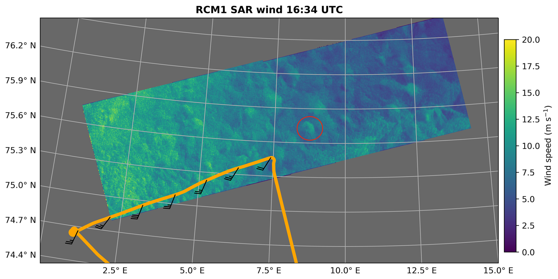
Figure 15 SAR imagery from RadarSat Constellation Mission 1 (RCM1) of the 10 m wind field in the vicinity of SL3 ∼30 min after the completion of SL3. The flight track is overlaid along with flight-level (300 m) wind barbs (knots). An example of a cold pool signature is circled, with an approximate width of 15 km.

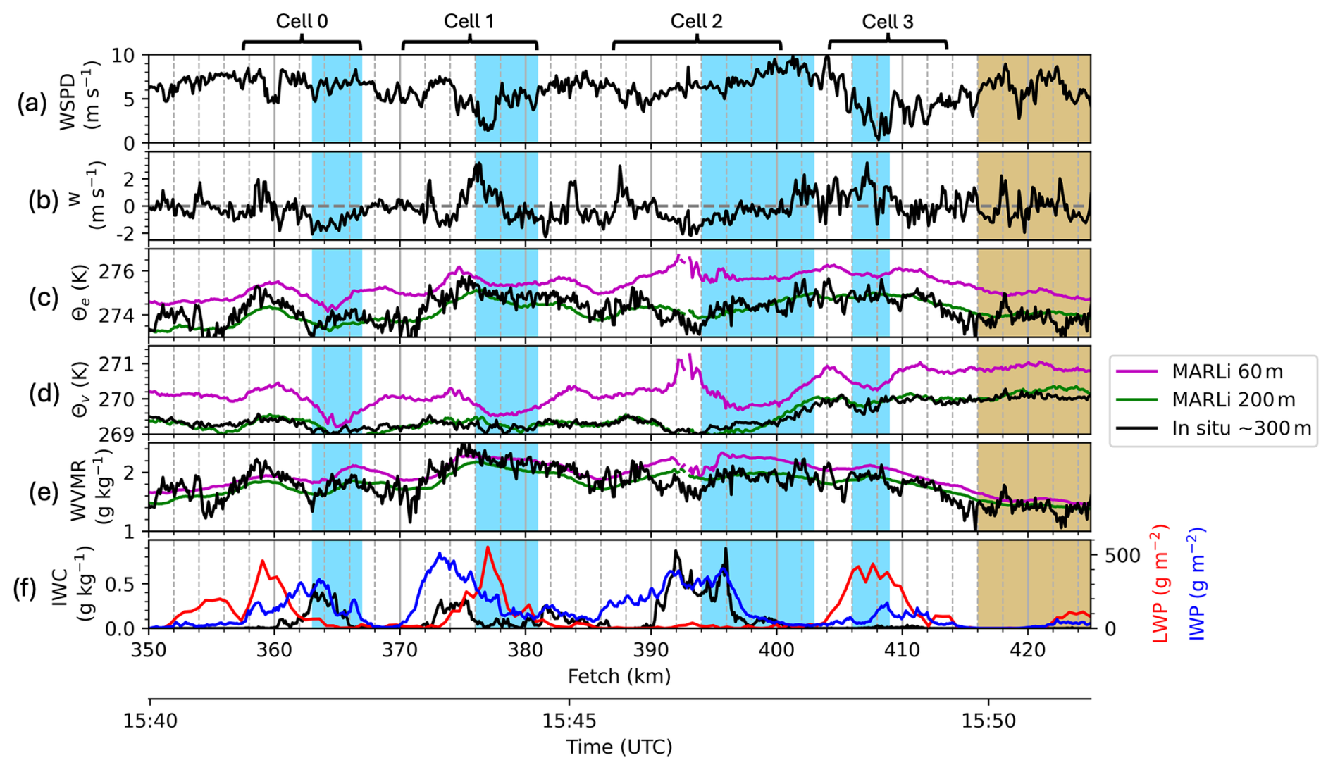
Figure 16 In situ flight level (300 m) (a) horizontal wind speed (WSPD), (b) vertical wind velocity (w), (c) θ_e, (d) θ_v, and (e) WVMR. (c)–(e) also include MARLi-derived values at 60 and 200 m altitude. (f) Retrieved LWP/IWP and in situ IWC. Cold pools are indicated in light blue and entrainment is indicated in gold. From km 391 to km 394, the lowest level MARLi-derived parameters (θ_e, θ_v, and WVMR) are impacted by heavy ice precipitation attenuating the MARLi signal.

Cell 0 near km 359 contains a narrow in-cloud updraft (<500 m wide; Fig. 14c) with maximum in situ vertical velocities reaching 2.0 m s⁻¹ (Fig. 16b), collocated with supercooled LWPs of 460 g m⁻² (Figs. 14g, 16f). The updraft is collocated with a decrease in horizontal wind speed, implying surface convergence (Fig. 16a). Downwind of the updraft, a precipitation shaft contains graupel and a few aggregates, with IWC reaching 0.49 g m⁻³ (Figs. 14a, b, 16f) and a surface cold pool (Δθ_v of −0.9 K; width of 4 km) located a couple km further downwind (km 366; Figs. 14d, 16d).

The in situ updrafts are even stronger in cell 1, reaching 3.2 m s⁻¹ near km 376 (also visible in a 10 m jump in the aircraft's altitude in Fig. 14d, e, f), collocated with LWPs of 550 g m⁻² (Fig. 16b, f). The updrafts are again collocated with a reduction in the horizontal wind speed from >5 to 1.4 m s⁻¹ (Fig. 16a), consistent with near-surface wind convergence. Upwind of the main updraft at km 374, an intense precipitation shaft with IWP reaching 510 g m⁻² coincides with flight-level IWC reaching a maximum of 0.33 g m⁻³ (Figs. 14a, g, 16f). Microphysical imagery includes abundant graupel (Fig. 14b). A cold pool (Δθ_v of −0.8 K; width of 5 km) is centered at km 378, again a few km downwind of the flight-level precipitation (Figs. 14a, d, 16d).

In contrast, cell 2 (near km 390) lacks both a well-defined updraft and liquid water, with maximum LWPs <40 g m⁻² (Fig. 14c, g). While in situ and Doppler vertical velocities reach 3 m s⁻¹ at km 388, the updraft does not reach the cloud base (Figs. 14c, 16b). A wide (6 km) precipitation shaft (IWP reaching 410 g m⁻²) contains the highest precipitation rate of all the open-cells, with IWC reaching 0.89 g m⁻³ consisting mostly of aggregates (Figs. 14a, b, g, 16f). The aggregate habit is consistent with the lack of supercooled water (Figs. 14g, 16f). Assuming a fall speed of 1 m s⁻¹, the maximum IWC equates to a liquid-equivalent precipitation rate of approximately 3 mm h⁻¹. The associated cold pool, the widest and most intense observed (Δθ_v of −1.3 K; width of 9 km), is centered at km 398, shifted (again) downwind, by 5 km, of the precipitation shaft center (Figs. 14a, d, 16d).

Cell 3 contains a broad updraft between km 404 and km 408 with a maximum in situ flight-level vertical velocity of 3.2 m s⁻¹ at km 407 (Figs. 14c, 16b). LWPs remain elevated >300 g m⁻² from km 406 to km 409 with a maximum of 440 g m⁻² (Figs. 14g, 16f). Little precipitation, mostly consisting of graupel, reaches the flight level (Fig. 14b). IWPs only reach 170 g m⁻², the least of all the open-cells (Figs. 14g, 16f). The corresponding cold pool is also the narrowest and weakest (Δθ_v of −0.7 K; width of 3 km) (Figs. 14d, 16d). Cell 3 borders the strongest entrainment event on the flight (ΔWVMR of −0.5 g kg⁻¹; width of 12 km) spanning from km 416 to km 428 (Fig. 14d, f), with a 5 km wide clearing from km 415 to km 420 (Fig. 14a).

While each observation is a snapshot in time, in combination they construct a visualization of how cells evolve in this cloud regime. The strong updrafts generating liquid water, but accompanied by little precipitation, suggest cell 3 is still developing. In cell 0 and cell 1, the strong updrafts are also associated with high LWPs adjacent to strong precipitation shafts containing graupel, indicating more mature cells. Cell 2, fully glaciated with dendrites and aggregates and no apparent in-cloud updraft, is more likely a decaying cell. Throughout the open-cells, IWP and flight-level IWC tend to be vertically aligned (Figs. 14a, g, 16f) consistent with minimal BL wind shear (Fig. 9). The cold pools tend to be located downwind of the main precipitation shafts, consistent with a cold pool expansion enhanced by the prevailing BL wind. Surface convergence supporting updrafts appears to be more common on the upstream edge of the cold pools, notably in cell 0 and cell 1 (Fig. 16a, b, d). The two-dimensional linear sampling of what is essentially a three-dimensional morphology may be introducing a possible sampling bias. Nevertheless, the contrast with the downstream generation of cloud mesoscale arcs within the tropical trade-wind regime (Zuidema et al., 2012) is of interest and will receive further attention. The cold pools furthermore do not thermodynamically decouple the BL (MARLi 60 m ${\mathit{\theta }}_{\mathrm{v}}/{\mathit{\theta }}_{\mathrm{e}}$ always exceeds MARLi 200 m ${\mathit{\theta }}_{\mathrm{v}}/{\mathit{\theta }}_{\mathrm{e}}$; Fig. 16c, d). As ice particles sublimate and form cold pools, the air can cool to its ice-bulb temperature, which has a similar magnitude to the more commonly used wet-bulb temperature (the heat of evaporation accounts for 88 % of the heat of sublimation). MARLi-derived 60 m wet-bulb depressions average to only 1.4 K during the open-cell segment of SL3, discouraging cold pool stabilization of the near surface air given the strong surface fluxes. θ_e is on average 1.1 K higher at 60 m than at 200 m, and presumably even higher at the surface. The cold pools do not appear to thermodynamically decouple the BL, in contrast to conceptualizations of the transition in warmer regions (Albrecht et al., 1995; Wyant et al., 1997; Sandu and Stevens, 2011; Yamaguchi et al., 2017). However, the convergence boundaries formed by the gust outflows initiate robust updrafts that likely further entrainment at cloud top.

7 Riming increases with fetch facilitating more precipitation

Over the course of SL13, the highest N_a, N_CCN and N_d reported during CAESAR (N_a of 650 cm⁻³, N_CCN of 680 cm⁻³ and N_d>600 cm⁻³), all decrease to less than 125 cm⁻³. These N_a, N_CCN and N_d are consistent within measurement uncertainties (Appendix C). Cloud droplet formation is primarily dependent on the activation of accumulation mode aerosols, which are depleted through entrainment with cleaner FT air and likely precipitation scavenging (Fig. 7; Appendix D). Sea spray aerosol production is estimated to be an order of magnitude less than the aerosol depletion rate (Appendix D). The transfer of Aitken mode aerosols through activation into larger accumulation mode particles is also unlikely to keep up with the removal of accumulation mode particles, even when buffered through entrainment of FT Aitken mode aerosol (Appendix D).

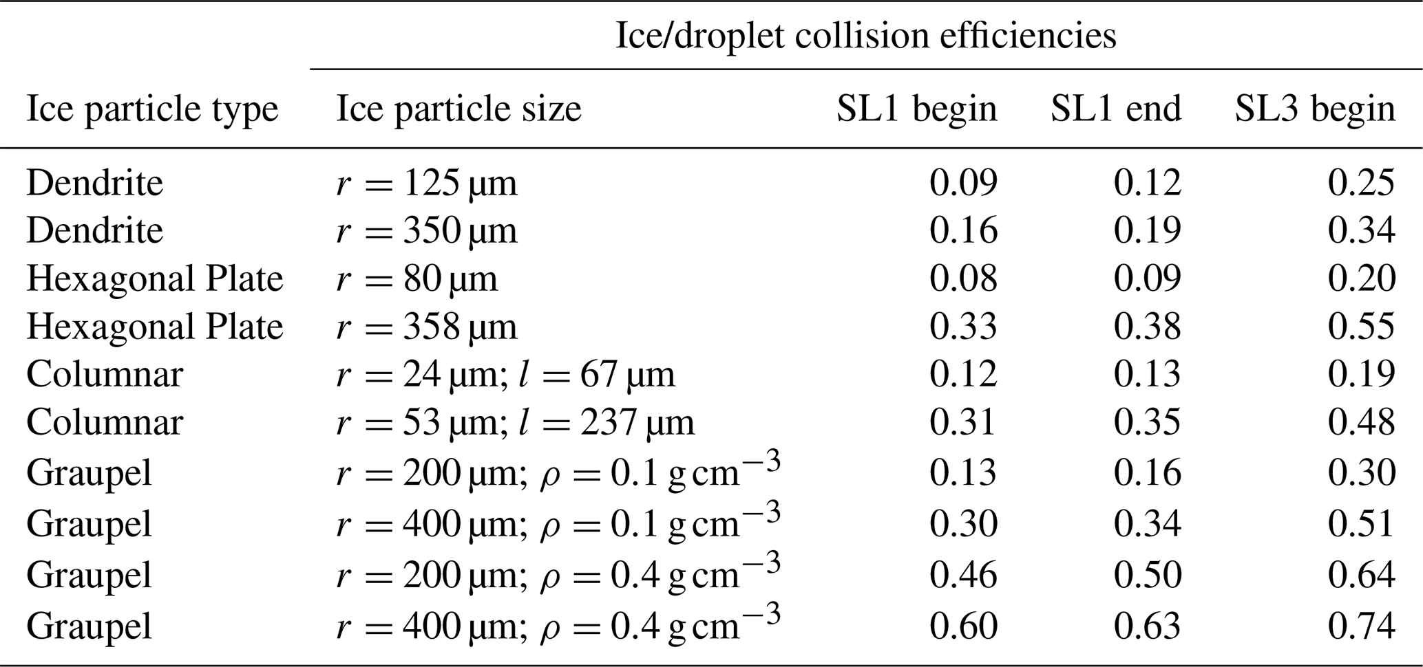
Here we discuss how reductions in N_CCN and N_d, and the resulting increasing droplet size, increase the riming efficiency with fetch. This in turn encourages more precipitation, as rimed particles fall faster than vapor-grown ice crystals, and thereby cold pools. In general, larger supercooled droplets and larger hydrometeors possess higher riming efficiencies. More specific values for the ice crystal collision/riming efficiencies as a function of ice crystal shape and size with the drop sizes measured during the three spiral profiles are provided in Table 2 using data from Wang and Ji (2000) and Khain et al. (2001).

The vertical profiles bounding SL1 (Fig. 12a, b) sampled aggregates and dendrites. Although some of the small ice at flight level appear rimed, dendrites are more common, indicating most ice particle growth is through vapor deposition. Despite the large LWPs, the small droplet sizes reduce the riming efficiencies (Lance et al., 2011; Norgren et al., 2018). No cold pools are observed during SL1, consistent with a light liquid-equivalent precipitation rate and slow fall speeds of dendrites. Ice particles with lower fall speeds are more likely to sublimate closer to the cloud base, moistening the sub-cloud layer, which helps maintain coupling between the ocean and the cloud layer, similar to liquid drops (Burford and Stewart, 1998; Feingold et al., 1996).

By the beginning of SL3, the N_d has decreased to 300 cm⁻³, the cloud droplet sizes have increased, and some supercooled drizzle is observed (Figs. 10c, 11). Although dendrites are present in the upper portion of the cloud, these become rimed at lower altitudes (Fig. 12c). Collision efficiencies increase by a factor of ∼2 between SL1 and the beginning of SL3 as drop sizes increase (Table 2). Cold pools nevertheless do not appear until after N_CCN decreases below 250 cm⁻³, after rapid BL growth (Fig. 14). By km 282, N_i exceeds 5 L⁻¹, and the ice habit suggests graupel (Fig. 14b, i). The LWPs have not increased since the beginning of SL3, indicating the dilution of N_CCN, by entrainment, may be impactful for increasing the ice production (Fig. 14g). By the time open-cell convection sets in (Fig. 14b), and during the ascent away from SL3 (Fig. 12d), numerous large graupel particles are present with diameters reaching 5 mm, and cold pools are plentiful (Fig. 14d). The increase in ice particle size and N_i after the transition to open-cells is also apparent in the composite F2DS and HVPS-3 ice particle size distribution (Fig. 17). The reduction in N_CCN accompanying the rapid BL growth prior to km 282 – likely brought about by entrainment facilitated by a weakening temperature inversion, subsequently accelerated by aerosol deposition – appears critical for setting up the internal conditions facilitating riming, more precipitation, and thereby the transition in cloud morphology.

Turbulence also increases the collision likelihood and thereby riming efficiency between ice particles and cloud droplets, particularly when both particles have similar fall speeds (Sheikh et al., 2024; Chellini and Kneifel, 2024; Li et al., 2026). In situ flight-level turbulent kinetic energy across a 100 s (10 s) moving window decreases from 1.9 m² s⁻² (1.0 m² s⁻²) during SL1, however, to 1.6 m² s⁻² (0.74 m² s⁻²) during the open-cell segment of SL3, as horizontal wind speeds decrease. This suggests turbulence may increase overall riming efficiency, but cannot explain increased riming with fetch.

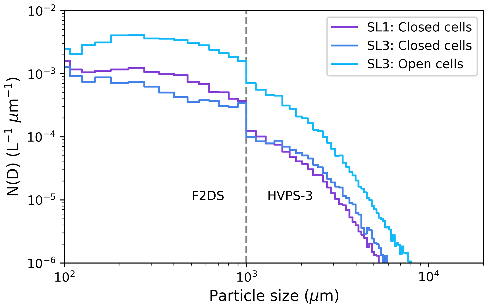
Figure 17 Composite F2DS (<100 µm) and HVPS-3 (>100 µm) ice particle size distribution averaged across segments of SL13, only including samples with N_i>0.01 L⁻¹. Line color indicates fetch using the scale in Fig. 7.

Table 2 Collision efficiencies of various ice particle types with supercooled droplets based on the observed drop size distribution during vertical profiles. Collision efficiencies of dendrites, hexagonal plates, and columnar ice crystals with various drop sizes are visually estimated from Figs. 6–8 in Wang and Ji (2000). Collision efficiencies of graupel are reported in Tables A1 and A2 in Khain et al. (2001).

8 Can we explain SIP?

N_INP during SL1 is comparable to other CAESAR flights, with concentrations around 2 L⁻¹ at an instrument aerosol processing temperature between −28 and −26 °C (Zuidema et al., 2026). N_INP decreases below the detection limit of the CFDC by the end of SL3 (Fig. 14i, Table 1). N_i is 50–500× higher than N_INP20 during closed-cell convection during SL1, consistent with SIP. Cloud temperatures are too low to support Hallett-Mossop splintering (Hallett and Mossop, 1974). Supercooled drizzle may be present during SL1, but only in small number concentrations that minimize the potential impact of freezing-induced-drop fragmentation. Another potential SIP mechanism is through ice-on-ice collisional breakup. One supporting observation is that, at an altitude of 750 m during the descent to SL1, N_i reaches a concentration of 6.5 L⁻¹ (500× higher than N_INP20), collocated with a spike in IWC to 0.25 g m⁻³ (and a depletion in LWC consistent with the enhanced removal of supercooled liquid through WBF processes and/or riming in the presence of higher N_i) at a temperature of −16.3 °C (Fig. 10a). This is near the temperature at which ice-on-ice collisional breakup is most effective (Takahashi et al., 1995; Vardiman, 1978). During the open-cell convection portion of SL3, N_i reaches concentrations of 12.5 L⁻¹, more than 5000× higher than N_INP20 (Fig. 14i, Table 1). Supercooled drizzle (>75 µm) at temperatures below −18 °C within both profiles bounding SL3 (Fig. 10c, d) potentially support both freezing-induced-drop fragmentation and ice-on-ice collisional breakup. Ice is also present in updrafts with in situ vertical velocities >1 m s⁻¹, crudely on par or exceeding the ice particle fall velocity (Fig. S2). N_i is greater than 0.1 L⁻¹ (1 L⁻¹) during 43 % (21 %) of the flight-level samples below open-cells with in situ vertical velocities >1 m s⁻¹. N_i values exceeding 100× ambient N_INP20 within updrafts indicates that their recirculation into open-cell convection could increase further N_i production (Korolev and Leisner, 2020; Lasher-Trapp et al., 2021).

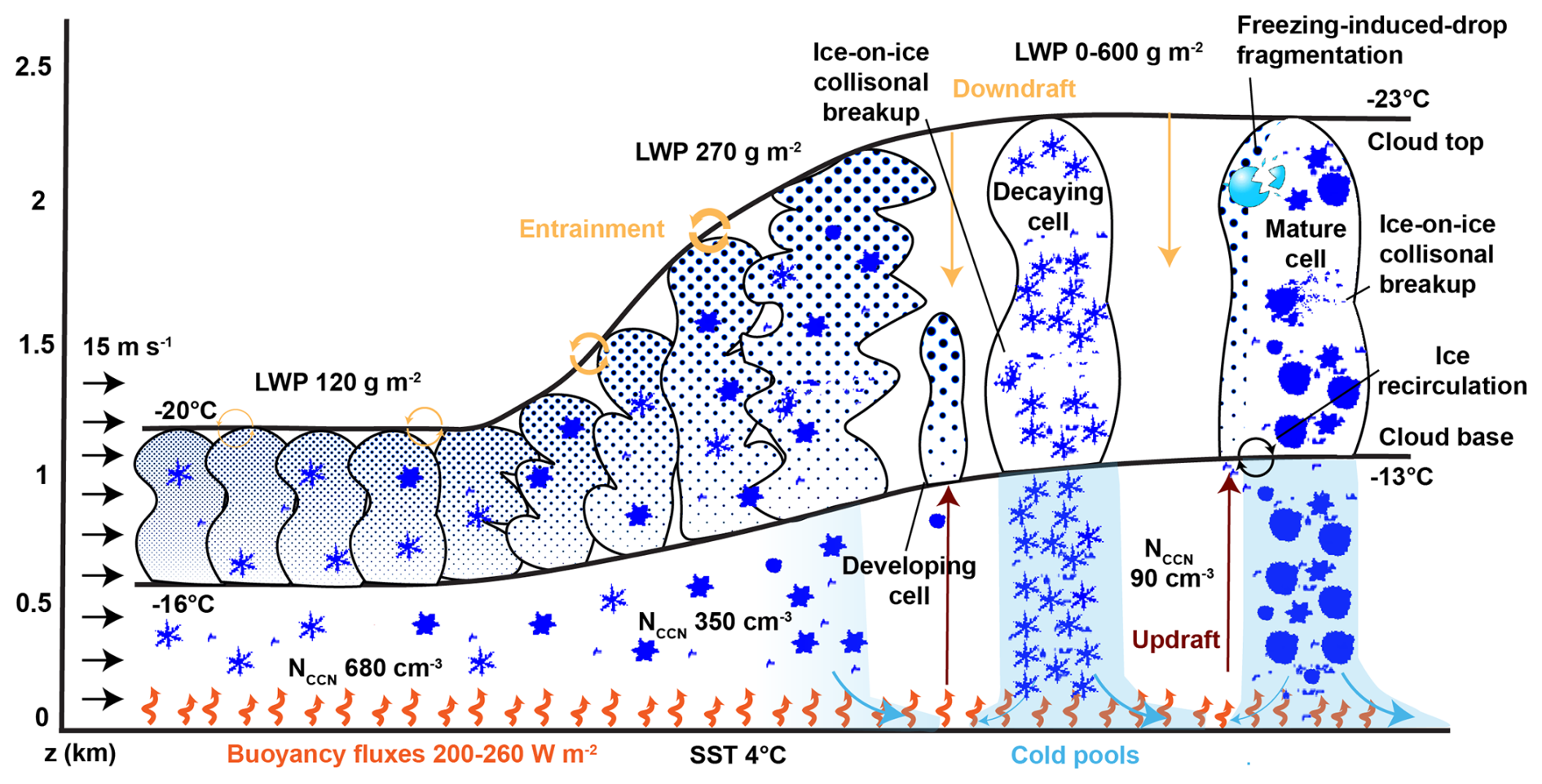
Figure 18 Schematic showing the microphysical and dynamical processes contributing to the closed-to-open cell transition.

9 Conclusions

The advanced and diverse instrumentation on-board the NSF NCAR C-130 during the CAESAR campaign characterized a closed-to-open cell transition within an MCAO made unusual by its high initial aerosol loading under cloud temperatures too cold to sustain Hallett-Mossop rime splintering, in the presence of surface buoyancy fluxes exceeding 250 W m⁻². In situ thermodynamic measurements confirm the synoptic pattern depicted by AROME-Arctic, supporting the inference that a cooling FT weakens the cloud-capping inversion, aiding the transition, as documented for warm-cloud transitions (Sandu and Stevens, 2011). The observations are summarized by the schematic in Fig. 18. Initially high CCN concentrations reduce the droplet diameters to <15 µm despite LWPs of 120 g m⁻². The riming efficiency is low, and SIP through freezing-induced-drop fragmentation is unlikely. N_i remains mostly <1 L⁻¹, and ice precipitation rates are too low to generate surface-based cold pools. A sharp cloud-top temperature inversion (∼10 K) limits BL growth by entrainment, despite strong surface fluxes. These factors support the maintenance of closed-cell convection.

By the beginning of SL3, as precipitation removes aerosol from the BL, and FT entrainment dilutes the BL aerosol number concentration, cloud droplet sizes increase. This supports increased riming. After a period of rapid BL growth likely facilitated by cooling FT temperatures that weaken the cloud-top inversion, SIP becomes more pronounced, with N_i>5 L⁻¹. Given the cloud temperatures, the SIP mechanisms are most likely freezing-induced-drop fragmentation and ice-on-ice collisional breakup (Korolev and Leisner, 2020), aided by recirculation. A deeper BL paired with increased riming efficiency increases precipitation rates, falling into an increasingly subsaturated sub-cloud layer, supporting the formation of cold pools.

A strength of this study is the ability of the MARLi-derived measurements of sub-cloud thermodynamics and microwave-derived cloud liquid water paths (Ephraim et al., 2025) to align with aircraft-measured vertical velocities, thereby depicting the cloud interactions with its environment. The cold pools appear to dynamically organize the convection through surface wind convergence, facilitating the transition to open-cell convection. The cold pools encourage convection at their upwind side at the expense of the downwind side, in contrast to trade-wind cumulus cold pools (Zuidema et al., 2012). However, the cold pools are weak and do not stabilize the sub-cloud air in the presence of the strong surface fluxes.

Our observations across the closed-to-open cell transition match some findings from Abel et al. (2017), with both cases observing liquid-dominated closed-cells, ice-dominated open-cells with localized LWP peaks associated with updrafts, and a decrease in aerosol number concentrations across the transition. This is despite the Abel et al. (2017) case including warmer cloud tops of −14.5 °C and weaker surface fluxes. In our case study, SIP occurs with cloud base temperatures $<-\mathrm{15}$ °C, outside the Hallett-Mossop rime-splintering temperature regime. Ice-on-ice collisional breakup and freezing-induced-drop fragmentation are hypothesized to dominate the SIP processes active during RF02. These SIP processes also likely contribute to the total N_i of the warmer Abel et al. (2017) case (Sotiropoulou et al., 2020; Karalis et al., 2022). A further distinction is that the BL during RF02 is much more polluted than that documented in Abel et al. (2017), with aerosol concentrations of 650 cm⁻³ before the transition. The reduction in the BL aerosol number concentration through cloud-top entrainment, facilitated by a weakening cloud-top temperature inversion, appears to be crucial for establishing the timing of the closed-to-open cell transition.

While we are not aware of significant caveats to this observational study, the representativeness of this case has not yet been established. Further modeling work will establish the relative impact of aerosols, thermodynamics, and SIP on the transition timing as well as distinguish the importance of the environmental controls from internal mechanisms.

Appendix A: Instrumentation

(Woods, 2026)(NSF/NCAR C-130 Team, 2025)(Woods, 2025)(Bansemer et al., 2025)(Perkins and Patnaude, 2024)(Perkins and Barry, 2025)(Snider, 2024a)(Petters and Cai, 2025a)(NSF/NCAR C-130 Team, 2025)(Snider, 2024b)(Petters and Cai, 2025b)(NSF/NCAR C-130 Team, 2025)(NSF/NCAR C-130 Team, 2025)(Grasmick et al., 2024)(Cruikshank et al., 2025)(Wang, 2025)(Ephraim and Zuidema, 2025)(Grasmick et al., 2026)(NSF/NCAR C-130 Team, 2026)(Villum Team, 2026)(Villum Team, 2026)(Villum Team, 2026)

Table A1 Instrument description, specifics, parameters and details of interest.

Appendix B: Entrainment derivation for SL1

Leg mean entrainment velocities (w_e) can be calculated with the following budget equation, derived from Ghate et al. (2019) and Kaser et al. (2017):

$$\begin{array}{}\text{(B1)}& \begin{array}{rl}{\displaystyle \frac{\partial Q}{\partial t}}& =-(\overline{u}-{\overline{u}}_{\mathrm{plane}}){\displaystyle \frac{\partial Q}{\partial x}}-\left(\overline{v}\right){\displaystyle \frac{\partial Q}{\partial y}}+{\displaystyle \frac{w_{\mathrm{e}}\mathrm{\Delta }{Q}_{\mathrm{inv}}}{H}}\\ & +{\displaystyle \frac{v_{\mathrm{d}}Q}{H}}+P_{\mathrm{net}}\left(Q\right)\end{array}\end{array}$$

with the x direction defined to align with the orientation of each flight leg. Q is a tracer concentration (O₃ or CO), $\overline{u}$ and $\overline{v}$ are the mean along-track and cross-track wind velocities respectively, ${\overline{u}}_{\mathrm{plane}}$ is the mean aircraft velocity, ΔQ_inv is the leg mean change in tracer concentration across the inversion, H is the leg mean boundary layer height, v_d is the deposition velocity, and P_net is any source or sink of the tracer. Since variations in Q are assumed to be primarily a function of fetch, $\frac{\partial Q}{\partial t}$ is assumed to be small. During SL1, since $\overline{v}$ is much smaller than $\overline{u}-{\overline{u}}_{\mathrm{plane}}$ and the FT airmass boundary is located more than 50 km to the southeast (small $\frac{\partial Q}{\partial y}$), $\left(\overline{v}\right)\frac{\partial Q}{\partial y}$ can also be ignored. Deposition and production of CO and O₃ are assumed to be negligible, simplifying to:

$$\begin{array}{}\text{(B2)}& (\overline{u}-{\overline{u}}_{\mathrm{plane}}){\displaystyle \frac{\partial Q}{\partial x}}={\displaystyle \frac{w_{\mathrm{e}}\mathrm{\Delta }{Q}_{\mathrm{inv}}}{H}}\end{array}$$

Flight-level CO concentrations decrease by 2.0 ppbv and O₃ increases by 1.6 ppbv over the 90 km fetch of SL1 (Fig. 13j). O₃ (CO) concentrations averaged 25 to 125 m above the inversion are well constrained, only changing from 43 to 45 ppbv (138 to 137 ppbv) between the profiles at the beginning and end of SL1 (Fig. 8a, b). The flight track is well-aligned with flight-level winds (flight-level along-track winds average 15.9 m s⁻¹ and cross-track winds average 0.4 m s⁻¹), and we can evaluate if the change in flight-level CO and O₃ is consistent with entrainment. Modeled AROME-Arctic subsidence velocities (w_s) average 10.7 cm s⁻¹ ∼200 m above cloud tops. Given the lack of boundary layer growth, w_e must balance the above-cloud large-scale vertical velocities, implying w_e averages to +10.7 cm s⁻¹, a similar magnitude to Tornow et al. (2022). This w_e value is unable to fully account for changes in tracer concentration: Equation (B2) with O₃ (CO) as a tracer produces w_e estimates of +60 cm s⁻¹ (+30 cm s⁻¹), or 3 to 6× higher than that estimated based on the lack of BL growth. We do not have a clear explanation, but neglect of mesoscale gradients in Q will contribute: the back-trajectories to Villum reveal less CO within the SL3-originating air mass than with the SL1-originating air mass (Fig. 6b). Another hypothesis is that the model-estimated large-scale subsidence is too weak, with the model also not able to produce enough boundary layer turbulence with which to balance the large-scale subsidence. This could also help explain why the modeled cloud tops are lower than those observed (Fig. 4c). The proximity to a sharp FT airmass boundary along with the imperfect alignment of SL3 with the mean BL wind (cross-track wind velocities average 9.3 m s⁻¹) prohibits a quantification of w_e.

Probability density functions (PDFs) of vertical velocities from segments of SL1 and SL3 reveal a positively-skewed distribution of updraft velocities reaching 3 m s⁻¹ at times with mean vertical velocities between −0.44 and −0.12 m s⁻¹ (Fig. C1a), a similar magnitude to w_e. Such vertical velocity distributions, of narrow updrafts and broader downdrafts, are more typical of cumulus than stratocumulus (Zhu and Zuidema, 2009).

Appendix C: Comparison of observed and modeled cloud droplet concentrations

Surprisingly large values of N_a, N_CCN, and N_d motivated an investigation of aerosol activation during RF02 (Snider et al., 2017). Aerosol measurements fitted to a three-mode function for the size distribution (Fig. 7) were input into the Julia wrapper of the Pyrcel adiabatic parcel model (Rothenberg and Wang, 2016) to calculate cloud droplet number concentration. The uncertainty in the three-mode aerosol fit is dominated by uncertainty in the MPSS number concentrations (±20 %; Cai et al., 2026; Liu and Deshler, 2003) and is propagated into Pyrcel. Calculated values of N_d were obtained for a range of updraft speeds and hygroscopicity (κ) values (Petters and Kreidenweis, 2007). Pyrcel is initialized at a temperature of −14 °C and a pressure of 900 hPa, the approximate conditions at cloud base (CB), and the aerosol size distributions are multiplied by ${\mathit{\rho }}_{\mathrm{CB}}/{\mathit{\rho }}_{\mathrm{STP}}$ to convert them to the pressure and temperature at cloud base. The vapor accommodation coefficient (α) is set to 1. Figure C1a indicates the supersaturations corresponding to the vertical velocities and aerosol size distributions for the three flight segments.

Table C1 Comparison of observed and modeled N_d for κ=0.4 and κ=0.8. Uncertainty in the observed aerosol number size distribution is propagated into Pyrcel, yielding a range of modeled N_d for each κ/leg. For SL1, there are two ranges of observed N_d corresponding to the two profiles bounding SL1.

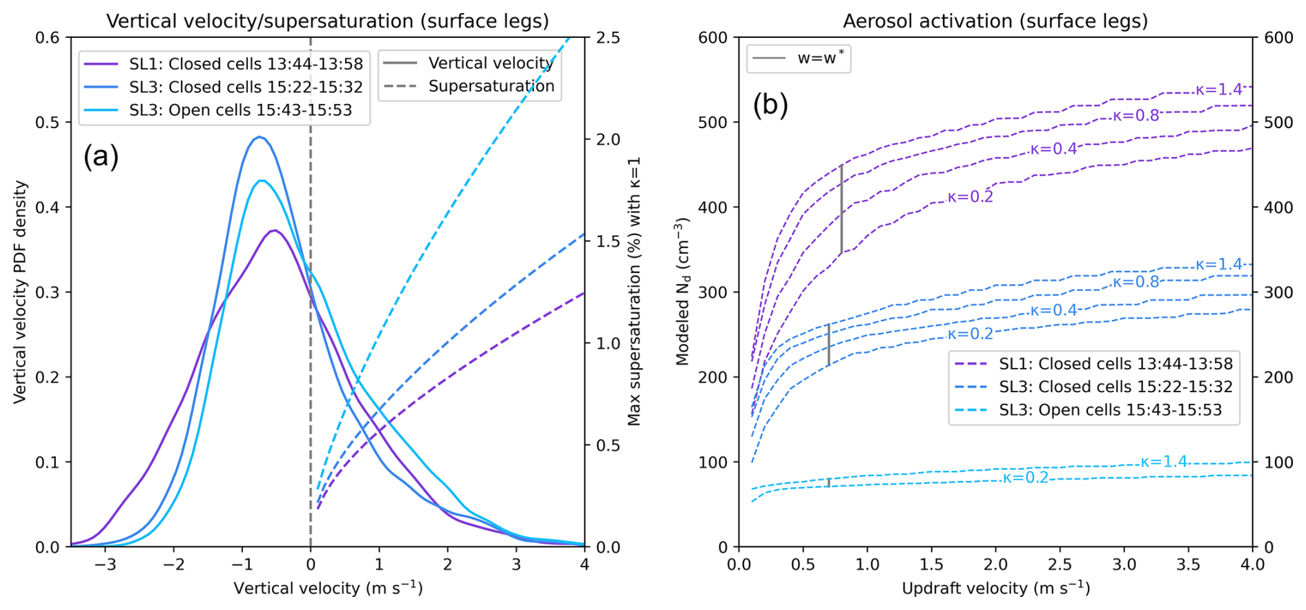
Figure C1 (a) PDF of the observed flight-level (300 m) vertical velocities for each flight segment along with the corresponding modeled supersaturations (using three-mode fit from Fig. 7 and setting κ=0.4, a similar κ observed in Williams et al., 2024) at different vertical velocities. (b) Modeled N_d (using three-mode fit from Fig. 7) as a function of updraft velocity between κ=0.2 and κ=1.4. Line color indicates fetch using the scale in Fig. 7. Gray lines indicate the modeled N_d at w^*.

The model-predicted N_d quickly attain their maximum values for a given hygroscopicity parameter (κ) between 0.2 and 1.4 for each flight segment at updraft velocities of 1 m s⁻¹ (Fig. C1b). The characteristic updraft velocity (w^*) is determined from $w^{*}={\mathit{\lambda }}^{*}\mathit{\sigma }$, where λ^* is a characteristic non-dimensional velocity (set to 0.65) and σ is the standard deviation of w (Morales and Nenes, 2010). Table C1 compares model-predicted N_d (at w^*) between κ=0.4 (the mean κ observed within MCAOs in Williams et al. (2024)) and κ=0.8 (the approximate κ of sulfate aerosols in Petters and Kreidenweis, 2007) with observed N_d. Uncertainty in observed N_d (assessed as ±20 %) can be caused by sizing uncertainty, particle coincidence (undercounting), and ice shattering (overcounting; Baumgardner et al., 2017). The NCAR C-130 deployed a modified CDP with a pinhole to reduce coincidence errors (Lance, 2012) and shatter-reducing tips. Modeled N_d during SL1 is 323–511 cm⁻³, consistent with N_d of 488–769 cm⁻³ observed during the profiles bounding SL1. The modeled N_d skews towards the lower end of observed N_d (Table C1), for reasons that remain unclear to us. During the descent to SL3, measured N_d is 242–362 cm⁻³ consistent with modeled N_d (196–302 cm⁻³; Table C1). Observed N_d (26–38 cm⁻³) is notably lower than modeled N_d (60–94 cm⁻³) towards the end of SL3 during open-cell convection (Table C1). This disagreement is likely a consequence of the spatial mismatch between when the aerosols and N_d were sampled. Entrainment can also reduce the measured N_d.

Appendix D: Do Aitken mode aerosols prolong the closed-cell convection?

The BL aerosol number size distribution at Villum includes only a weak Aitken mode (Fig. 7). By the beginning of SL1, the initially clear-sky air mass has deepened and become cloud-filled, and the Aitken mode aerosol is much more clearly developed (Fig. 7). The free troposphere is dominated by Aitken mode aerosols (Fig. 7). The BL Aitken mode aerosol can therefore originate from marine emissions (Kecorius et al., 2019) and/or from cloud-top entrainment. Over the pristine Southern Oceans, FT Aitken mode aerosol, formed as new particles within the outflow of cyclones, contribute to the N_d through activation after entrainment (McCoy et al., 2021). In contrast, within the more polluted MCAOs over the northwest Atlantic, entrainment from the free troposphere primarily dilutes the accumulation mode aerosol population, and the FT Aitken mode aerosol population contributes little to the N_d (Tornow et al., 2022, 2025). Here we provide a preliminary aerosol budget to assess the importance of the FT Aitken mode population to the high documented N_d values.

The BL N_ait is 150 cm⁻³ at the beginning of SL1, while the BL N_acc reaches 500 cm⁻³ (Fig. 7). Overall, N_CCN, N_a, and rBC concentrations are higher in the BL than the FT (Figs. 7, 8). Assuming an entrainment velocity at the BL top of 10 cm s⁻¹ (see Appendix B) along with unvarying FT N_ait and N_acc, dilution by entrained FT air will decrease BL N_ait during SL1 by 22 ${\mathrm{cm}}^{-\mathrm{3}}{\mathrm{h}}^{-\mathrm{1}}$, and N_acc by 145 ${\mathrm{cm}}^{-\mathrm{3}}{\mathrm{h}}^{-\mathrm{1}}$. At the same time, the sea spray aerosol flux parameterization applied within Wyant et al. (2022), adapted from Clarke et al. (2006), estimates ocean fluxes of both N_ait and N_acc during SL1 of approximately 3 ${\mathrm{cm}}^{-\mathrm{3}}{\mathrm{h}}^{-\mathrm{1}}$, given a satellite-retrieved 10 m wind speed of 13 m s⁻¹ (Fig. 15), dispersed through a 1230 m deep BL.

The robust updrafts can also activate the BL Aitken mode aerosol and transfer these to the larger accumulation mode aerosol centered at a diameter of 100 nm (Fig. 7). The Pyrcel activation model (see Appendix C) estimates 2 cm⁻³ Aitken mode particles and 398 cm⁻³ accumulation mode particles become activated throughout an eddy overturning timescale of 27 min (respective activation fractions of 2 % and 60 %), assuming a κ of 0.4 following Williams et al. (2024) and a characteristic vertical velocity of $w^{*}=\mathrm{0.77}$ m s⁻¹ for SL1. This transfer corresponds to a rate of 5 ${\mathrm{cm}}^{-\mathrm{3}}{\mathrm{h}}^{-\mathrm{1}}$. The combination of these three processes decreases N_ait at a rate of 24 ${\mathrm{cm}}^{-\mathrm{3}}{\mathrm{h}}^{-\mathrm{1}}$ during SL1.

The distance from the midpoint of the SL1 aerosol segment (km 55) to the midpoint of the first SL3 aerosol segment (km 263) is 208 km (Fig. 1). Cloud-level winds range from 13–15 m s⁻¹, decreasing with distance. Assuming stationarity, the distance corresponds to 4–5 h of travel by the cloudy air mass. Over that time period, assuming the N_ait net loss remains steady, the estimated N_ait decreases by 96–120 cm⁻³. This is higher than an observed decrease of 50 cm⁻³ (Fig. 7). Loss of Aitken mode aerosol through wet scavenging is not considered, and the assumption of stationarity may be incorrect. Nevertheless, this assessment suggests the closed-cell convection is primarily maintained by the high concentrations of BL accumulation mode aerosol, similar to the northwest Atlantic (Tornow et al., 2025). While Aitken mode aerosol by themselves can contribute to the observed N_d during SL1, the entrainment that brings Aitken mode aerosol into the BL is more effective at diluting the more-influential accumulation mode aerosol. The BL N_ait decreases significantly along SL3 (Fig. 7), and entrainment of FT Aitken mode particles may become a source and help buffer the BL Aitken mode particle population. FT and BL aerosol number concentrations are not as well constrained during SL3, however, due to the proximity to a FT airmass boundary to the south (Fig. 4a, b). While the closed-cell convection is likely primarily maintained by the high concentrations of BL accumulation mode aerosol, further modeling work is needed to assess the contribution of FT Aitken mode aerosol for the transition taking place later (e.g., Wyant et al., 2022).