Spring-summer atmospheric circulation and boundary layer processes modulating aerosol and cloud characteristics over the coastal Northeast Pacific during EPCAPE

Observations collected during the ARM Eastern Pacific Cloud Aerosol Precipitation Experiment (EPCAPE) for the period spanning April to September 2023 (spring and summer) at Scripps Pier in La Jolla, California (32.8669° N, 117.2569° W) were used to investigate the regional-scale atmospheric factors that control the variability of predominant marine low clouds and aerosols in the coastal boundary layer. Using Self-Organizing Maps (SOMs) applied to ERA5 sea level pressure and near-surface wind fields, we classify the synoptic evolution of the subtropical anticyclone into 9 regimes. This regime categorization highlights the following dominant features in Northeast Pacific: (1) regimes that capture the evolution of the anticyclone in terms of magnitude (strong vs. weak) and location (coastal vs. offshore), with their corresponding transitions in boundary layer wind strengthening and large-scale subsidence (regimes: 1–3 vs. 6–8), (2) a second dominant feature characterized by an anticyclone with its core at the northwestern edge of the domain, resulting in modest sea level pressure changes near Scripps Pier (regimes 6–8), (3) patterns with a weakened subtropical anticyclone south of Scripps Pier and a midlatitude cyclone further north (regimes 4 and 5), and (4) an additional regime that captures anomalies that minimally depart from the climatological mean (regime 9). GOES-18 satellite cloud retrievals reveal that regimes associated with an anticyclone core closer to the EPCAPE coastal site (regimes 1–4) is associated with reduced low-cloud fraction, shallower clouds, and low liquid water path (LWP) along the shoreline; whereas regimes with a west/north-westward-displaced anticyclone combined with a weak coastal inland low-pressure feature (regimes 6–8) that support extensive stratocumulus with higher LWP and elevated cloud tops. Variability in the aerosol distribution is also controlled by the synoptic scale processes. Regimes with a relatively weak anticyclone centered adjacent to the Scripps Pier (regime 4) generally feature the highest concentrations of particles with diameter ≤ 0.1 µm, associated with a stable boundary layer and stagnation under weak winds. Regimes with anticyclone strengthening farther offshore (regimes 6–8) have relatively lower aerosol concentrations. The partial inconsistency in the evolution of the cloud droplet number concentration (N_d) and aerosol concentration indicates that the variability in boundary layer turbulence is a critical component that explains the aerosol activation into N_d.

1 Introduction

The Northeast Pacific (NEP) stratiform cloud regime is a key climatological feature over the subtropics, playing a central role on the Earth's radiation budget (Hartmann et al., 1992; Wood, 2012) and exerts a climate feedback with the large-scale sea surface temperature and atmospheric circulation (e.g., Clement et al., 2009). Coastal Southern California experiences diverse synoptic weather patterns driven by the coastal topography and large-scale circulation. The subtropical high dominates in spring and summer, generating strong onshore flow that enhances marine layer clouds and coastal cooling (Raphael, 2003; Clemesha et al., 2017). In contrast, fall and winter witness a wider range of weather patterns, with frequent synoptic-scale transitions of anticyclonic and cyclonic circulation of varying extent and magnitude. These changes dramatically modulate cloud variability, giving rise to convective systems especially in frontal regions, and synoptically forced stratocumulus clouds under conditions with strong post-cyclonic subsidence (Weaver and Ramanathan, 1997). These circulation shifts generate stark contrasts in coastal meteorology, pollutant dispersion, and cloud variability (Lu and Turco, 1994, 1995). Furthermore, the diurnal land-sea breeze interacts with the synoptic forcing. Weak synoptic forcing allows land-sea breezes to dominate, while katabatic winds originated from a high-pressure system (Santa Ana winds) disrupt these cycles, enhancing offshore pollutant transport and reducing cloud coverage (Abel and Hall, 2010). In contrast, low-pressure conditions strengthen the offshore flow, deepen the marine atmospheric boundary layer (MBL), and increase the cloud cover (Lebassi-Habtezion et al., 2011).

The coastal southern California is particularly impacted by transport of polluted air from industrial regions like Los Angeles and Long Beach (Husar and Patterson, 1980; Husar et al., 1977). Moreover, pollution transport extends offshore over the stratocumulus cloud-topped marine atmospheric boundary layer during Santa Ana wind events (Abel and Hall, 2010), directly affecting the marine stratocumulus clouds. Conversely, synoptic onshore flow brings pristine marine aerosols inland, dramatically changing the local aerosol composition (Maneenoi et al., 2025; Han et al., 2025). The diversity in chemical composition and wide range of aerosol variability makes this region a unique observatory for investigating aerosol pathways and modes of variability over a coastal region situated next to densely urbanized areas. Moreover, advection of continental aerosols over the adjacent ocean can potentially impact the evolution and radiative properties of the NEP stratocumulus cloud deck. In this respect, a fundamental mechanism of aerosol-cloud interaction is through an increase in cloud droplet number concentration (N_d) mediated by an increase of cloud condensation nuclei (CCN) under conditions of enhanced aerosol loading (Bellouin et al., 2020 and references therein). The positive correlation between CCN and N_d have been observed in several studies (e.g., Sorooshian et al., 2019; Painemal et al., 2017), with the radiative implications manifested in an increase of albedo at the top of the atmosphere documented from satellite observations (Painemal, 2018). It has been hypothesized that changes in N_d can trigger multiple feedbacks and rapid cloud adjustments that can alter the cloud properties (precipitation, water content, thickness, among other); however, their magnitudes remain highly uncertain (Bellouin et al., 2020).

An important factor contributing to uncertainties in the quantification of the aerosol indirect effect is the fact that clouds primarily respond to changes in the local atmospheric state, which in turn also modulate the microphysical interactions between aerosol and clouds. Indeed, Chen et al. (2014) and Zhang et al. (2022) highlight the importance of accounting for meteorological factors for assessing aerosol-cloud interactions (e.g., atmospheric stability and humidity). For the NEP, data collected during the MAGIC campaign (Lewis, 2016) along with reanalyzed meteorological fields show that the coastal California low-level jet as a key mechanism transporting aerosols from North American continent to the northeast Pacific. Furthermore, Painemal et al. (2015) found a negative correlation between 1000 hPa zonal wind and N_d, underscoring the influence of large-scale meteorology in transporting aerosol from coastal regions to the open ocean in the NEP.

Cognizant of the knowledge gaps in the characterization of clouds and aerosols in the atmospheric boundary layer of coastal California, the Department of Energy's Atmospheric Radiation Measurement (ARM) program deployed the ARM Mobile Facility at Scripps Pier (32.8669° N, 117.2569° W) in La Jolla (California) during the Eastern Pacific Cloud Aerosol Precipitation Experiment (EPCAPE; Russell et al., 2025). This year-long field campaign, conducted from mid-February 2023 to mid-February 2024, provided comprehensive high-resolution observations of aerosols, clouds, precipitation, and atmospheric state. Being a downwind coastal site, Scripps Pier is ideally situated to observe the interactions between continental and marine air masses, and boundary layer clouds in the NEP.

Here, we describe the synoptic regimes that modulate cloud variability and aerosol characteristics over the coastal Southern California for the period spanning April through September 2023 corresponding to Southern California spring (April–June) and summer (July–September), a period characterized by the frequent presence of stratocumulus clouds. To this end, we employ self-organizing maps (SOM) – an unsupervised neural network method – to categorize meteorological regimes using fields from the Fifth Generation ECMWF reanalysis (ERA5). In addition, Satellite ClOud and Radiation Property retrieval System (SatCORPS) cloud products derived from the 18th Generation Geostationary Operational Environment Satellite (GOES-18) and ground-based in-situ and remote sensing measurements for the study period from the EPCAPE campaign at Scripps Pier are combined to analyze the factors that link the atmospheric circulation with cloud and aerosol characteristics. By leveraging EPCAPE observations, this research provides a novel approach to linking large-scale weather patterns with localized atmospheric processes. The paper is structured as follows: Sect. 2 outlines the EPCAPE in-situ and remote measurements, satellite cloud observations, and reanalysis data. Section 3 covers atmospheric regime classification using SOM. Section 4 describes meteorological, cloud, and aerosol properties within these atmospheric regimes. Section 5 outlines the summary and discussion.

2 Datasets and methodology

The key dataset for this study was collected by the ARM's Mobile Facility deployed at Scripps Pier during EPCAPE. ERA5 and SatCORPS GOES-18 are primarily used for describing the regional scale context of the EPCAPE observations. In the following, we describe the dataset used in our study.

2.1 ARM observations and products

2.1.1 Cloud boundaries

Cloud base height (CBH) is estimated from a laser ceilometer Vaisala CL31 (CEIL: Zhang et al., 2023; Morris, 2016), with a 16 s sampling and a vertical resolution of 10 m. The typical accuracy of CBH measurements is within ±30 m for low clouds, though uncertainties increase at higher altitudes or in the presence of fog, aerosols, or precipitation. Ceilometer data were also used to estimate the hourly cloud occurrence frequency for low altitude clouds, hereafter referred to as cloud frequency fraction (CFF) and computed by counting the number of cloudy observations relative to the total sampling in an hour.

The vertically pointing Ka-band ARM Zenith Radar (KAZR: Widener et al., 2012; Feng et al., 2024), provided cloud top height (CTH) measurements throughout the campaign. We used the KAZR Active Remote Sensing of Clouds (KAZRARSCL: Johnson et al., 2023) Value Added Product (VAP) for determining the cloud height, with the vertical resolution of 30 m and a 4 s sampling.

2.1.2 Liquid water path and cloud optical thickness

The 3-channel Microwave Radiometer (MWR3C) provided LWP retrievals at 1 s interval throughout the campaign. MWR3C measures brightness temperatures at three frequencies (23.8, 30, and 89 GHz) which are sensitive to atmospheric water vapor and liquid water. The LWP is retrieved using the updated Microwave Radiometer RETrieval (MWRRETv2; Gaustad and Zhang, 2023) algorithm which follows the physical retrieval method developed by Turner et al. (2007) and Gaustad and Turner (2009) and is provided as ARM VAP. The inclusion of the 89 GHz channel, with its enhanced sensitivity to low liquid water content, improves retrievals for clouds with small LWP. We limit the sampling to boundary layer clouds by only retaining observed clouds with KAZR cloud tops below 2 km. The occurrence of thin clouds is minimized by removing samples with LWP < 5 g m⁻² and CFF < 20 %. To reduce the retrieval and measurements uncertainty, we evaluate non-precipitating clouds, by filtering out the measurements during surface precipitation events, (excluded datasets with rain fraction > 0), which accounted < 1 % of total. This filtering effectively eliminates periods of substantial surface precipitation while retaining cases of light drizzle aloft that evaporate before reaching the ground (this behavior is frequently observed in subtropical marine stratiform clouds) and remain part of the dataset. Finally, to ensure comparability across instruments with different sampling intervals, all cloud and aerosol datasets for the Scripps Pier are aggregated onto a common 1 h time grid.

Ground-based ARM N_d is computed from the ARM Cimel Sunphotometer (CSPHOT: Fairless et al., 2023; Chiu et al., 2010, 2012) cloud optical thickness (τ) and MWRRETv2 LWP following Painemal et al. (2017), enabling robust analysis of cloud microphysical properties from ground-based data. A second ground-based ARM N_d utilized here is NDROP N_d available as ARM VAP product (McComiskey et al., 2009) calculated using Multifilter Rotating Shadowband Radiometer derived τ and MWRRETv2 LWP following Boers and Mitchell (1994).

2.1.3 Aerosol observations

Continuous range of aerosol number concentration (N_a) and particle size distribution are obtained from merged Scanning Mobility Particle Sizer (SMPS) and Aerodynamic Particle Sizer (APS) measurements, available as MERGEDSMPSAPS VAP (Beddows et al., 2010; Shilling and Levin, 2023; Shilling, 2023). The SMPS measures the high-accuracy aerosol number size distribution, in the particle diameter range from 0.01 to 0.5 µm, by sizing particles based on their electrical mobility diameter using a differential mobility analyzer (DMA) and by counting particles using a condensation particle counter (CPC). The APS measures larger atmospheric particles in the diameter range of 0.5 to 20 µm, based on their aerodynamic diameter using the time-of-flight principle. Datasets are available for the entire EPCAPE time frame at 5 min interval except for a short duration (19 September through 23 October) of missing data.

Chemical composition and mass concentration of species aerosols such as organics, sulfate, nitrate, ammonium, and chloride are derived from Aerosol Chemical Speciation Monitor (ACSM: Shilling and Levin, 2024; Maneenoi et al., 2025) and are available at a 30 min interval.

2.1.4 Cloud Condensation Nuclei

The cloud condensation nuclei (CCN) number concentration was measured on Scripps Pier by DOE ARM using a Cloud Condensation Nuclei Counter (CCN-200, DMT: Enekwizu et al., 2023). The CCN counts aerosol particles after growing them at water supersaturations of 0.1 %, 0.2 %, 0.4 %, 0.6 %, 0.8 %, and 1.0 % during a 1 h cycle. This dataset is available for 25 May 2023 to 14 February 2024. A scaling factor of 1.67 (Berta et al., 2025) was applied to correct for a leak upstream of the instrument inlet that diluted CCN number concentrations with air from inside the air-conditioned instrument van based on closure with composition and comparisons to the Mt. Soledad site (Dedrick et al., 2026). This analysis focuses exclusively on CCN measurements at supersaturations (SS) of 0.1 % and 0.2 % because they are more representative of the environmental conditions at the Scripps Pier (Dedrick et al., 2026).

2.1.5 Meteorological observations and models

The reanalyzed atmospheric dataset used in this study corresponds to ERA5 (Hersbach et al., 2020). ERA5 combines various observations from satellite and weather stations with advanced numerical weather prediction models to provide consistent and complete global records of atmospheric, oceanic, and land-surface conditions. Comprehensive atmospheric datasets are produced hourly at a horizontal resolution of 31 km (with spatial resolution of 0.25° × 0.25°) and 137 vertical levels extending from surface to 0.01 hPa. The hourly datasets, as well as daily and monthly mean are also available to download at https://doi.org/10.24381/cds.adbb2d47 (Hersbach et al., 2023). The single-level products sea level pressure and sea surface temperature, as well as near-surface (975 hPa) winds, free-tropospheric (750 hPa) temperature, humidity, and winds from the vertical profiles are utilized in this study.

Backtrajectories are obtained from ARMTRAJ (Silber, 2023; Silber et al., 2025), an ARM VAP. ARMTRAJ consists of an ensemble of HYSPLIT forward and backward trajectories derived from hourly ERA5 ensemble reanalysis at 0.25° resolution for up to 10 d. ARMTRAJ is initialized at different levels, including surface (ARMTRAJ-SURF, 10 m), boundary layer top (ARMTRAJ-PBL), and cloud layer (ARMTRAJ-CLD). These trajectories provide information on the origin of air masses and are used to understand the source and transport path of aerosol and trace gas distributions. Here, we primarily utilize PBL backtrajectories to identify the possible transport processes for different atmospheric regimes at the Scripps Pier. ARM Eddy Correlation (ECOR) system provides half-hour measurements of the surface fluxes and carbon dioxide (Cook, 2025; Sullivan et al., 2025). The ECOR system deployed at the Scripps Pier include a fast-response, 3D wind sensor (sonic anemometer) to record the orthogonal wind components and the speed of sound, which is used to derive the air temperature, and an open-path infrared gas analyzer (IRGA) to obtain the water vapor density and CO₂ density. Turbulent Kinetic Energy (TKE) derived from ECOR measurements available in ARM EPCAPE Doppler Lidar profile statistics (DLPROFWSTATS: Newsom et al., 2019) is utilized here to understand the boundary layer turbulence. Lastly, the analysis is complemented with high-resolution vertical profiles of temperature, humidity, wind speed, and wind direction collected from radiosondes launched at Scripps Pier (Keeler et al., 2023; Keeler, 2025). During April through September 2023, radiosondes were launched at 6 h intervals (local times approximately 06:00 a.m., 12:00 a.m., 06:00 p.m., and 12:00 p.m. LT).

2.2 SatCORPS GOES-18 satellite cloud products

Satellite retrievals are derived from the GOES-18's Advanced Baseline Imager (ABI) using a family of algorithms referred to as the Satellite Cloud and Radiation Property Retrieval System (SatCORPS). These algorithms are adapted from those developed by the Clouds and Earth's Radiant Energy System (CERES) to ingest radiances from geostationary sensors (Minnis et al., 2008, 2011, 2023). For this study, the native resolution pixel retrievals at ∼ 2 km are produced half hourly and gridded to 0.20° × 0.20° grid over the EPCAPE domain, defined here as the region covering the box of 28–43° N and 112.5–130° W. These gridded data are averaged according to their cloud height into low (height < 2 km), middle (2 km < height < 6 km), and high (height > 6 km) clouds. The cloud products include cloud fraction (CF), cloud optical depth (τ), droplet effective radius (r_e), LWP, temperature, and height. Given the large uncertainties and limitations of optical retrievals during nighttime (optical depth and droplet effective radius) we only retain daytime observations with solar zenith angle (SZA) less than 70°. To minimize retrieval artifacts from thin or broken clouds, we apply additional screening criteria in our analysis: CF > 10 %, τ > 2 (Grosvenor et al., 2018). Also, we filter-out grid boxes with cloud top temperature (CTT) lower than 273.15 K and specifically select for this analysis averaged retrievals corresponding to the low height category (< 2 km) with LWP range of 5–250 g m⁻² to limit the analysis to stratus and stratocumulus clouds and minimize retrieval uncertainties. On average these filters reduce the data availability by approximately 60 %, however, provides a cleaner and more physically consistent sample for evaluating regime-dependent aerosol–cloud relationships. The SatCORPS algorithm computes LWP from the retrieved cloud optical thickness (τ) and droplet effective radius (r_e) using the relation (Nakajima and King, 1990; Nakajima et al., 1991):

$$\begin{array}{}\text{(1)}& \mathrm{LWP}=(\mathrm{4}/\mathrm{3})\cdot {\mathit{\rho }}_{\mathrm{w}}\cdot \mathit{\tau }\cdot r_{\mathrm{e}}/Q\end{array}$$

where ρ_w is the density of liquid water and Q is the cloud extinction efficiency, approximately 2.0. The algorithm follows the bispectral approach and simultaneously retrieves τ and r_e using the 0.64 and 3.9 µm reflectances under the assumption of a 1-D, plane-parallel, homogeneous cloud layer. Because passive satellite sensors are most sensitive to the upper few optical depths of the cloud, the retrieved r_e corresponds to values near cloud top rather than the vertically averaged droplet radius, and the LWP computed following Eq. (1) would be an overestimate in marine stratiform clouds where typically r_e increases from cloud base to cloud top. To account for this bias, an adiabatic correction following Wood and Hartmann (2006) is applied to the LWP computation. The adiabatic LWP is computed using Eq. (2) given below, and accounting for the adiabaticity reduces the LWP derived from Eq. (1) by a factor of ($\mathrm{5}/\mathrm{6}$) or 17 %.

$$\begin{array}{}\text{(2)}& {\mathrm{LWP}}_{\mathrm{adb}}=(\mathrm{5}/\mathrm{9})\cdot \mathit{\tau }\cdot r_{\mathrm{e}}\end{array}$$

The cloud droplet number concentration (N_d) is estimated following the approximation for subtropical clouds in Painemal and Zuidema (2011) based on the adiabatic approximation. This approach assumes that liquid water content increases linearly with height and incorporates an adiabatic factor of 1.0.

$$\begin{array}{}\text{(3)}& N_{\mathrm{d}}=\mathrm{1.4067}\times {\mathrm{10}}^{-\mathrm{6}}\left[{\mathrm{cm}}^{-\mathrm{1}/\mathrm{2}}\right]\cdot {\mathit{\tau }}^{\mathrm{1}/\mathrm{2}}/r_{\mathrm{e}}^{\mathrm{5}/\mathrm{2}}\end{array}$$

Since numerous studies have reported a systematic positive bias in r_e derived from geostationary and sun-synchronous imagers of about 20 % relative to in-situ data (e.g. Minnis et al., 2021; Painemal et al., 2023, 2025), we apply a 0.8 correction factor to the r_e values before computing N_d, to minimize error propagations in Eq. (3).

2.3 Self-Organizing Maps for synoptic regime classification

Self-Organizing Maps (SOMs; Kohonen, 1982; Kohonen, 1990; Bishop, 1995; Vesanto and Alhoniemi, 2000; Kohonen, 2001; Haykin, 2009) is an unsupervised machine learning technique designed to cluster and visualize high-dimensional data by projecting it onto a two-dimensional grid while preserving the topological relationships inherent in the data. The SOM algorithm groups similar data patterns into neighboring neurons on the grid, with each neuron i represented by a weight vector w_i. This weight vector is iteratively adjusted during training to reflect the distribution of the input data, ensuring that patterns with similar features are positioned close to each other on the grid. Recent studies emphasize the effectiveness of SOMs in synoptic climatology and environmental analysis (Hewitson and Crane, 2002; Sheridan and Lee, 2011; Jiang et al., 2013; Pearce et al., 2014; Juliano and Lebo, 2020; Painemal et al., 2023). The training process of SOMs involves several steps as described in Haykin (1999, 2009):

1. Initialization: The weighting vectors of the neurons are initialized randomly for better convergence. Each neuron in the map is represented by a weighting vector with the same dimensionality as the input data.

2. Determine the winning neuron i: For each input vector x, the algorithm calculates the Euclidean distance between the input vector and each neuron's weight vector. The neuron with the smallest distance to the input is selected as the winner, ${\arg }_{i}min\parallel x-w_i\parallel$, where w_i represents the weight vector of the ith neuron.

3. Adapting weights: The winner and its neighboring neurons are updated to move closer to the input vector. The weight update for a neuron i at time t is given by:

   $$w_i(t+\mathrm{1})=w_i\left(t\right)+\mathit{\eta }\left(t\right)h\left(i\right)(x-w_i(t\left)\right);$$

   where η(t) is the learning rate which typically decreases over time and h(i) is the Gaussian neighborhood function, which determines how much a neuron is influenced based on its distance from the winner.

4. Decay of Learning Rate and Neighborhood: Both the learning rate η(t) and the neighborhood radius σ(t) decrease over time to allow fine-tuning in later training stages: $\mathit{\eta }\left(t\right)=\mathit{\eta }\mathrm{0}{e}^{-kt}$, $\mathit{\sigma }\left(t\right)=\mathit{\sigma }\mathrm{0}{e}^{-kt}$; where η0 and σ0 are the initial learning rate and neighborhood radius, and k is a time constant controlling the decay rate.

5. Iteration: This process is repeated over multiple epochs, iterating through the dataset either sequentially or in batches. Early epochs focus on global organization with larger neighborhoods and higher learning rates, while later epochs fine-tune the local structure, resulting in a topologically ordered map where similar input patterns are mapped to nearby neurons, allowing for the visualization and clustering of complex datasets.

We utilized MiniSOM (Vettigli, 2018), a Python based implementation of SOM, which leverages the NumPy framework for computational efficiency, making it particularly suitable for analyzing moderate-sized datasets with minimal dependencies.

3 Results

To interpret the characteristics of aerosols, clouds, and meteorology over Southern California coast during EPCAPE spring and summer (April–September) months, we first identified the dominant synoptic patterns (9 regimes) using a SOM classification applied to SLP and 975 hPa winds. For these 9 regimes, we evaluate the dynamic and thermodynamic variables (vertical velocity at 500 hPa, relative humidity, BL stability and coupling state, turbulence, etc.) to characterize the MBL and governing large-scale circulation over the NEP and the Scripps Pier pattern using ERA5 reanalysis meteorology and ARM in-situ radiosonde measurements. In the section following, we evaluate the spatial pattern in cloud properties (low-cloud fraction, cloud droplet number concentration, liquid water path, and cloud top height) from SatCORPS GOES-18 satellite retrievals and ARM EPCAPE ground based observations of cloud properties including KAZR CTH, Ceilometer CBH, MWR LWP, etc. for the Scripps Pier and discuss how the key meteorological features drive these regime specific cloud properties. We assess particle number concentration from ARM in-situ merged SMPSAPS measurements to understand how synoptic regimes modulate aerosol variability, and their correspondence to CCN, and N_d. Additionally, we explore the role of boundary layer turbulence in observed N_d and accumulation mode N_a. Finally, to understand the aerosol transport pathways, we analyze the ACSM aerosol species measurements and ARM PBL backtrajectories for the 9 synoptic regimes.

3.1 Regional-scale classification

The first step in the synoptic clustering is to select the meteorological fields that will be used for the pattern classification. To this end, we consider a variable that represents the large-scale features over the region of study and a second parameter that captures local features along the coast. The clear choice that satisfies these conditions over the coastal NEP are, respectively, sea level pressure (SLP, e.g., Juliano and Lebo, 2020) and boundary-layer wind fields at 975 hPa (e.g., Abel and Hall, 2010). We also experimented with adding the 500 hPa geopotential and 850 hPa winds fields to SOM, which resulted in negligible changes in the clustering (not shown). Next, 11 years (2012–2022) of daily April through September SLP and winds are normalized by subtracting the 30 d moving average at each 0.25° grid point and divided by the 30 d running standard deviation. This normalization ensures that the algorithm primarily discerns meaningful meteorological patterns rather than seasonal changes and extreme modes of variability. Alternative anomaly normalizations, such as spatial averaging methods used in previous studies (e.g., Juliano and Lebo, 2020), were tested but were found to disproportionately weigh land-ocean differences in SLP variability. Secondly, to determine the spatial domain extent best suited for capturing meteorological variability relevant to the NE California coast, we tested three domains of varying sizes: a large domain (10–50° N, 160–100° W), a medium-size domain (20–50° N, 140–110° W), and a small domain (30–40° N, 125–115° W). We found that the clustering for the large domain was dominated by large-scale changes in SLP far offshore, showing modest differences in meteorological conditions for the coastal region near Scripps Pier. In contrast, the small domain captured many more details that tended to yield spatially noisy patterns that lacked consistent features. The medium-sized domain (30° × 30°) provided the most representative patterns for the Southern California region, effectively capturing the dominant synoptic-scale features. Finally, we tested several objective methods to determine the optimal number of SOM nodes. First, we used the silhouette score to evaluate the uniqueness of patterns across different node selections. This metric informs about how close each point in one cluster is to the points in the neighboring cluster, with score ranging between −1 and 1. A higher score (> 0.5) suggests the clusters are well-separated, whereas a negative score suggests wrong cluster assignment. In our case, the scores ranged from 0.065 for six clusters to 0.021 for nine clusters, degrading further with higher node counts, which rendered this method unsuitable. Second, we applied a two-step clustering approach: initially generated an SOM classification with 20 clusters (4 × 5 nodes) and then regrouped with K-means to reduce the number of patterns. However, this approach produced slightly noisier and less coherent patterns. Ultimately, the optimal number of nodes/clusters was chosen visually by testing several configurations (4 × 5, 4 × 4, 3 × 4, 3 × 3, etc.) to ensure clear classification of regional synoptic features. A 3 × 3 SOM (nine nodes) provided distinct, coherent synoptic regimes, striking a balance between capturing variability and maintaining interpretability. Moreover, this 3 × 3 SOM configuration effectively captures the evolution of the SLP discerned by the 4 × 5 SOM, as corroborated by comparing the normalized sea level pressure fields in Fig. 1 and Fig. S1 in the Supplement.

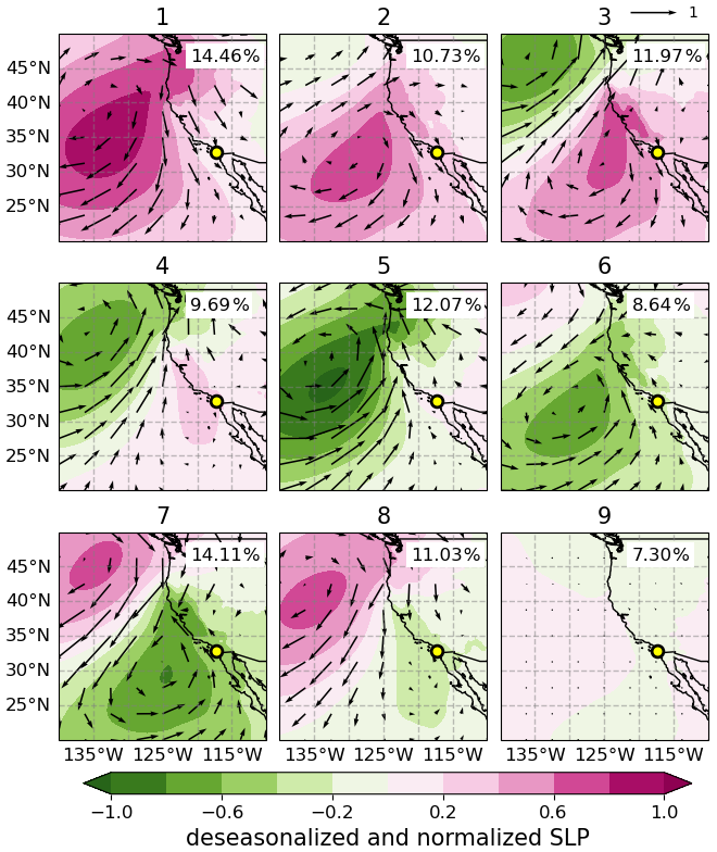
Figure 1 11-year daily April–September mean composite maps of deseasonalized and normalized SLP and 975 hPa wind fields for the 9 regimes determined from SOM. Clusters are labelled from 1 to 9, and their frequency of occurrence is listed in percentage on the upper-right corner of each map. The yellow circle represents the location of the EPCAPE main site Scripps Pier.

The 9 patterns (regimes) determined by the SOM classification is shown in Fig. 1. These patterns capture the dominant synoptic features over the NEP and coastal Southern California and are arranged to reflect a progression in anticyclone/cyclone movement. It is interesting to observe a coherent transition of the anticyclone-cyclone system that resembles the evolution of weather disturbances. Pattern 1 displays pronounced high-pressure anomaly centered northwest of the Scripps Pier with anticyclonic offshore wind anomalies, and occur 14.46 % of the time (the highest frequency among all regimes). Patterns 2–8 feature the development, eastward advancement, and southeastward dissipation of a cyclonic system. More specifically, pattern 2 features an anticyclone strengthening with its center positioned about 10° W of Scripps Pier, and with intensified offshore anticyclonic anomalous flow, whereas a cyclonic system develops at the northwest corner. Pattern 3 is characterized by an anomalous anticyclone closer to the Pier, as the anomalous cyclonic pattern strengthens. Pattern 4 depicts a diminished anomalous anticyclonic signature now centered even closer to the Pier with modest winds, with the cyclonic center shifting further south relative to pattern 3. Pattern 5 displays a predominant cyclonic feature centered directly west of Southern California, producing broad anomalous onshore winds across the region. Pattern 6 captures a moderate anomalous low-pressure system advancing southeastward covering much of the domain, accompanied by enhanced anomalous onshore flow. The anomalous low-pressure pattern further advances along the direction in pattern 7, generating strong anomalous onshore flow. Pattern 8 shows a modest anomalous low-pressure feature over Southern California while anomalous anticyclone displaced further south in pattern 7. Pattern 9 presents minimal changes in SLP and winds and, thus, represents climatological features.

3.2 General features of the synoptic regimes

We use SLP and wind fields in the boundary layer (975 hPa, ∼ 300 m a.s.l.) and the free troposphere (750 hPa, ∼ 2.5 km a.s.l.) for describing the circulation and transport pathways during April–September 2023 of EPCAPE campaign. Table S1 summarizes the monthly occurrence frequency of the 9 regimes for the period of study. In addition, low-cloud control variables examined here include vertical velocity in pressure coordinates at 500 hPa (ω₅₀₀), 750 hPa relative humidity (RH₇₅₀), and lower tropospheric stability (LTS). LTS is defined as the difference in potential temperature (θ) between 750 hPa and the surface (similar to Klein and Hartmann, 1993). The meteorological fields for each regime are depicted as mean composites in Fig. 2, and as anomalies relative to the monthly running mean in Fig. 3. While the discussion is mainly guided by Fig. 2, Fig. 3 provides quantitative information of magnitude changes of the deseasonalized fields. The SLP patterns in Fig. 2 features a dominant anticyclone with varying values of magnitude and extent anticipated by Fig. 1. In contrast, regime 1 depicts the strongest development of the anticyclone, with boundary layer winds exceeding 10 m s⁻¹ near the Scripps Pier. Similarly, the high-pressure system is well developed in regimes 7 and 8, but with their core displaced farther northwest than in regime 1, and with wind speeds greater than 10 m s⁻¹. Regime 2 shows a moderately developed anticyclone but with relatively modest deseasonalized values (Fig. 3a), with its center aligned with the latitude of Scripps Pier. Regimes 1, 2, 7, and 8 feature wide areas of subsidence (ω₅₀₀ > 0) and consistent free tropospheric drying (RH₇₅₀ < 30 %) over the ocean. For these regimes with intense mean and deseasonalized anticyclone, we observe a strengthening of the coastal winds parallel to the coast south of 40° N. Notably, these coastal winds tends to be stronger in the boundary layer (Fig. 2a, arrows) than in the lower free troposphere (Fig. 2b, arrows), which is a common feature of the coastal low-level jet around Cape Mendocino (40.4° N, Parish, 2000). Regimes 3, 4, and 5 are unique in that they feature a weak cyclonic circulation north of 40° N, with westerly winds north of 35° N, and concomitant with 500 hPa ascents (Fig. 2a, ω₅₀₀ < 0). Regime 9 features the climatological mean pattern, as discussed in Sect. 3.1.

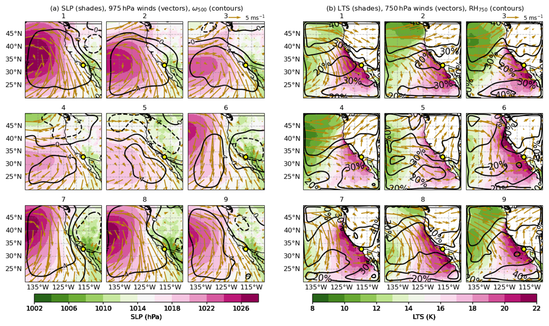
Figure 2 Composite maps of mean meteorological fields for the nine synoptic regimes identified for April–September 2023. (a) Sea level pressure (SLP; color shading), 975 hPa winds (vectors), and pressure vertical velocity at 500 hPa (× 10⁻² Pa s⁻¹; black contours). (b) Lower tropospheric stability (LTS; shading), 750 hPa winds (vectors), and relative humidity at 750 hPa (RH₇₅₀; black contours).

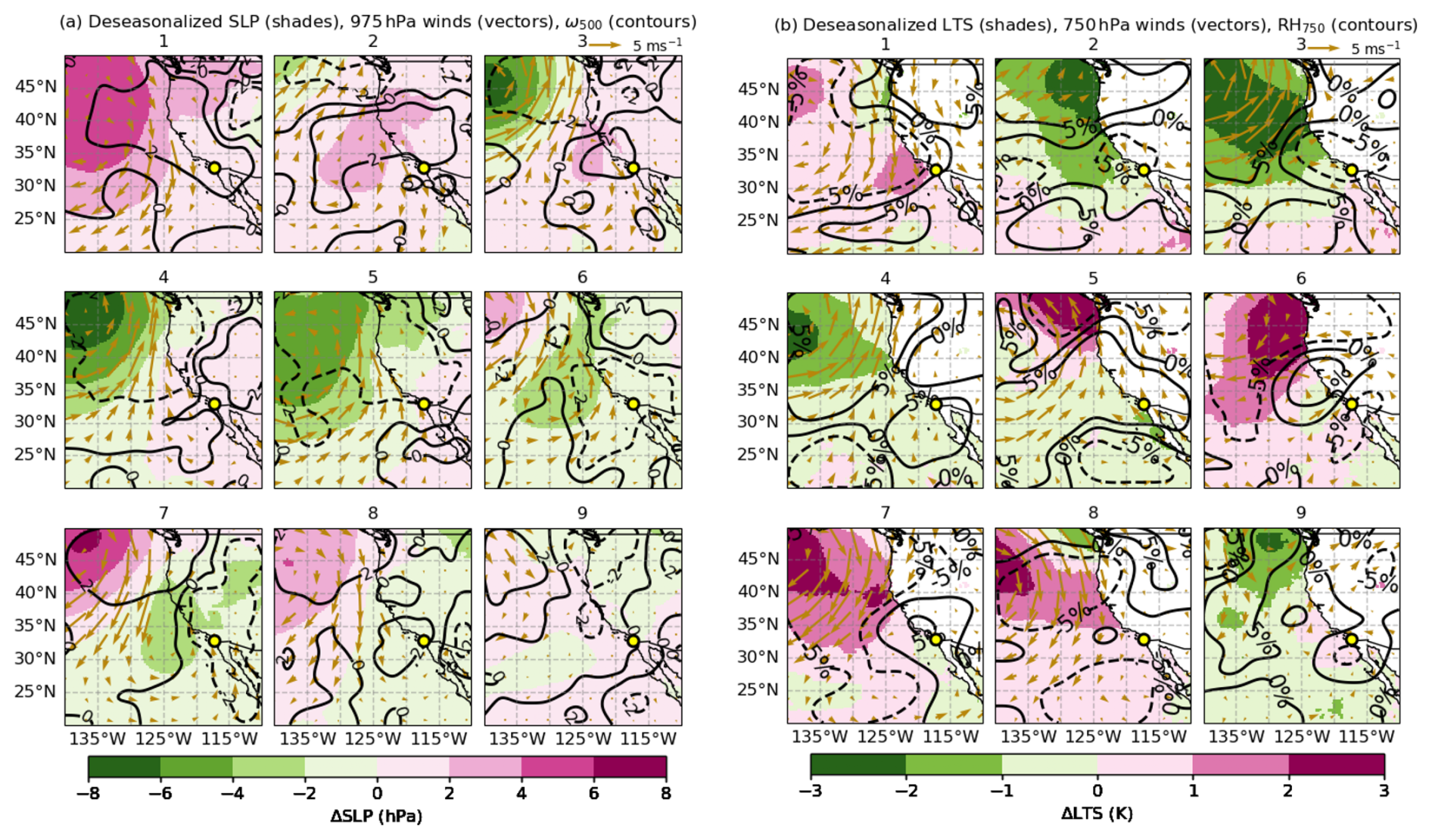
Figure 3 Deseasonalized meteorological fields (using the 30 d running mean) for the nine synoptic regimes identified for April–September 2023. (a) SLP (color shading), 975 hPa winds (vectors), and pressure vertical velocity at 500 hPa (× 10⁻² Pa s⁻¹; black contours). (b) LTS (shading), 750 hPa winds (vectors), and relative humidity at 750 hPa (RH₇₅₀; black contours).

In terms of 750 hPa winds, consistent with the strengthening of the anticyclonic and cyclonic circulation, regimes 3–5 exhibit a dominant zonal component, suggesting transport of marine air masses inland. For 1, 2, and 8 (anticyclones), winds run parallel to the coast, potentially contributing with a mixture of continental and marine air masses to Scripps Pier. For regimes 6–7, the wind direction shows dominant meridional component. There is an increase in LTS for all the regimes with values > 20 K for the broad coastal area south of 40°, except that regimes 4 and 5 show slightly lower LTS. It is, nevertheless, surprising that deseasonalized anomalies in Fig. 3b show modest variability for the same coastal area, especially near Scripps Pier, with inter-regimes differences smaller than 3 K, and with unclear connections with the atmospheric circulation depicted in Fig. 3a. This implies that the patterns of the mean LTS in Fig. 2b primarily reflect seasonal changes rather than synoptic-scale processes. As we will see in the following sections, the modest variability in LTS cannot explain changes in the cloud fields, confirming the poor correlation between LTS and cloud cover at synoptic scales reported by a number of studies (e.g. Klein et al., 1997).

3.3 Atmospheric structure derived from Radiosonde observations at Scripps Pier across nine synoptic regimes

After providing a regional description of the atmospheric variability over the coastal NEP, we center our attention on the thermodynamical properties of the lower troposphere derived from radiosondes observations collected during EPCAPE at Scripps Pier. Figures 4 and 5 provide, respectively, median and deseasonalized atmospheric profiles for each regime. The boundary layer for all regimes is statically stable, with mean LTS values ranging between 15–20 K (Fig. 4a). Regime specific features are more easily observed in the θ anomaly (deseasonalized) profiles in Fig. 5a. Regimes experiencing an anomalous anticyclonic (e.g., regimes 3, 4, 5) or cyclonic circulation (e.g., regimes 7, 8) around the Pier depict negative θ anomalies (about −1 K) within the boundary layer, while the other regimes generally show positive θ anomalies. In terms of relative humidity, most regimes maintain high RH (> 80 %) in the boundary layer with the expected sharp decrease in the free troposphere (Fig. 4b). Median RH profiles suggest shallow MBL tops (< 1 km) in most regimes, while regimes 7 and 8 feature slightly deeper boundary layers extending beyond 1 km. These regimes are associated with anomalous cyclonic dominant synoptic conditions that promote upward moisture transport, particularly regimes 7 and 8, which maintains elevated RH throughout the lowest 2 km, consistent with moist northwesterly flow and enhanced ascent (Zhou et al., 2015). In addition, stronger boundary-layer turbulence from intensified winds and upper level wind reversal enhancing entrainment under relatively weaker static stability, likely contribute to the boundary-layer deepening observed in regimes 7 and 8. Consistently, these regimes also exhibit positive RH anomalies. Regimes 1 and 2 are typically associated with anomalous high-pressure and associated subsidence in coastal regions and exhibit weak negative RH anomalies.

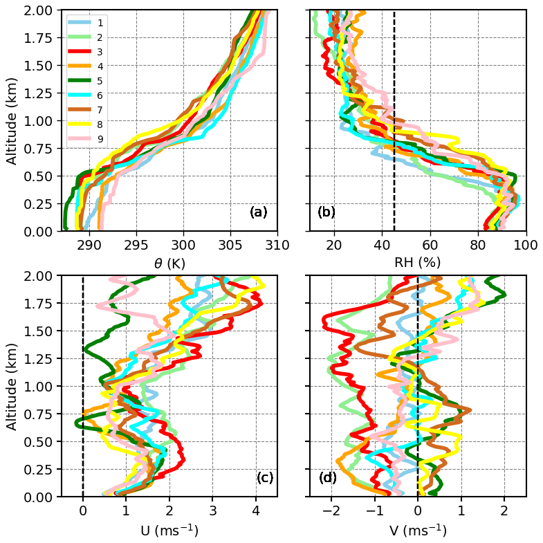
Figure 4 Regime-composite median vertical profiles of thermodynamic variables for the lowest 2 km from radiosonde observations for April to September 2023, for the nine synoptic regimes. (a) Potential temperature (θ), (b) relative humidity (RH), (c) zonal wind (U), and (d) meridional wind (V). Vertical dashed line in panel (b) indicate 45 % RH threshold depicting BLH. The width of the 95 % confidence intervals (CIs) of these profiles suggests that most regimes are significantly different from each other, except for regime 6 where the width of CIs of potential temperature profiles were large.

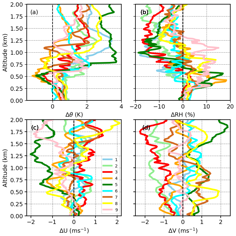
Figure 5 Regime-based median profiles of the deseasonalized thermodynamic variables for the lowest 2 km for April to September 2023, computed as deviations from the 30 d running mean. (a) Potential temperature anomaly (Δθ), (b) relative humidity anomaly (ΔRH), (c) zonal wind anomaly (ΔU), and (d) meridional wind anomaly (ΔV). Dashed vertical lines represent the zero-anomaly reference.

Wind profiles in Fig. 4c generally feature a westerly component with magnitude of less than ∼ 2 m s⁻¹ in the boundary layer. Meridional wind (V) profiles are more revealing of the position and strength of the anticyclone: Most regimes are dominated by a modest but persistent northerly flow (negative V), consistent with cold air advection and coastal subsidence typical of summertime marine stratus regimes (Parish, 2000). On the other hand, regimes 7 and, to a lesser extent, 8 display southerly flow (positive V), indicative of warm, moist advection into the coastal boundary layer, likely enhancing turbulence and transport of aerosol from southern shore to the Pier (Painemal et al., 2013).

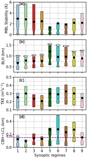
Specific properties that characterize the boundary layer are presented in Fig. 6. Boundary-layer stability is quantified from radiosonde observations using a MBL stability metric, defined as the potential temperature difference between 700 m and the surface. Regime-mean values range from 5 to 10 K, with larger values indicating a more stable MBL and smaller values reflecting enhanced turbulence. Although the medians are below 1 K, regimes 1–4 exhibit larger mean values (∼ 2 to 3 K) and wider upper-quartile range (> 6 K), representing the stable boundary layer. Conversely, regimes 5-8 exhibit weakest stability, with mean values (≤ 2 K), consistent with a less stratified boundary layer and enhanced turbulence mixing. The boundary layer height (BLH) is simply estimated as the altitude for which RH drops below 45 % (Bretherton et al., 2010). BLH exhibits moderate variability across regimes (Fig. 6b). Consistently, regimes 1-4 exhibit shallowest boundary layers with mean BLH ∼ 750 m, consistent with stronger subsidence that inhibits vertical development of the MBL. In contrast, regimes 5–8 are characterized by substantially deeper boundary layer. Deeper MBL is typically conducive to enhanced vertical cloud extent and increased LWP, a trend consistent with the regime-specific cloud structures to be discussed in Sect. 3.4 and 3.5.

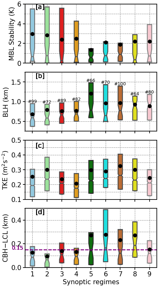
Figure 6 Boxplot of (a) MBL stability metric, (b) boundary layer height (BLH), (c) turbulent kinetic energy (TKE), and (d) CBH–LCL difference, for the nine synoptic regimes for April to September 2023 at Scripps Pier. Boxes show interquartile range with medians marked by horizontal lines, and black circles denote the mean. Notches represent the 95 % confidence interval of the median, according to the test described in Krzywinski and Altman (2014). The magenta dashed line in panel (d) marks the 150 m threshold used in Jones et al. (2011) to identify decoupled boundary layers. The number of samples for each regime is shown in panel (b).

Figure 6c shows the distribution of TKE across the synoptic regimes, highlighting substantial regime-dependent modulation of boundary-layer turbulence. TKE is highest in regimes 5–8 with mean values of approximately 0.3–0.35 m² s⁻², indicating the favoring of strong boundary layer mixing. In contrast, regimes 1–4 (with the exception of regime 2) exhibit lower mean TKE of about 0.20–0.25 m² s⁻², representing a weakly turbulent boundary layer. Regime 9 shows intermediate behavior, with turbulence levels ranging between those of the shallow, stable regimes and the deeper, less stable regimes. Lastly, regime 7 depicts moderate mean TKE, which is also regime with deeper and a weakly stratified BL.

The difference between cloud base height (CBH) and the lifting condensation level (LCL) provides insight into the degree of cloud-boundary layer coupling (Fig. 6d). A CBH–LCL separation exceeding approximately 150 m (highlighted by the dashed line) typically signifies decoupled conditions, wherein the cloud layers are no longer directly connected to the surface moisture supply and below-cloud turbulence (Wood and Bretherton, 2004; Jones et al., 2011). Regimes 5–8 frequently exhibit upper quartiles with CBH–LCL values that exceed the 150 m threshold, indicating frequent decoupling. Conversely, regimes 1–4 maintain tightly clustered CBH–LCL distributions near or below 150 m, indicative of well-coupled marine boundary layers. In such regimes, cloud bases closely follow the lifting condensation level, enhancing aerosol–cloud interactions and generally supporting higher N_d as discussed in the Sect. 3.6, assuming sufficient aerosol availability (Wood, 2012).

3.4 Cloud characteristics for synoptic regimes

To characterize the link between synoptic-scale meteorology and low-level clouds along the Southern California coast during the EPCAPE, we create regime composites of SatCORPS GOES-18 cloud properties. Figure 7 presents the spatial mean distributions of key low-level cloud properties: low-level cloud fraction (LCF), N_d, LWP, and CTH. Figure 8 shows the corresponding spatial anomalies of these variables, calculated relative to the 30 d running mean climatology. Figures 7a and 8a show that low-level clouds are less frequent when the subtropical anticyclone center is closer to the coastal Southern California or if it is weaker (regimes 1–5). In these regimes, the fractional low-cloud amount is below 50 % along the shoreline and increased to 70 %–80 % over the southern offshore domain. About 10 %–20 % of mid+high cloud incidence (Fig. S2) in these regimes along the coastline indicates that the corresponding low-cloud reduction is partially attributed to obscuration of higher clouds in the satellite sensor field of view. Notably, regime 5 is partially linked to synoptic storm systems in midlatitudes, indicating that deeper convection and frontal systems may play a dominant role in shaping the clouds in this regime. In contrast, regimes characterized by an offshore high pressure and a developing low pressure over land (regimes 6–8) display greater low cloud amount exceeding 70 % along the southern California shoreline and wider offshore. Indeed, the positive deseasonalized anomalies in LCF were above 10 % in these regimes and this increase in low-cloud coverage is consistent with wide regions with subsidence and a reinforcement of the northerly winds (Fig. 2a), two factors that favor the strengthening of the thermal inversion (Myers and Norris, 2013; Wood, 2012). Regime 9, the regime closest to climatological neutrality, displays average LCF values of ∼ 70 %, but shows negative anomalies (∼ 5 % to 10 %) around the EPCAPE site.

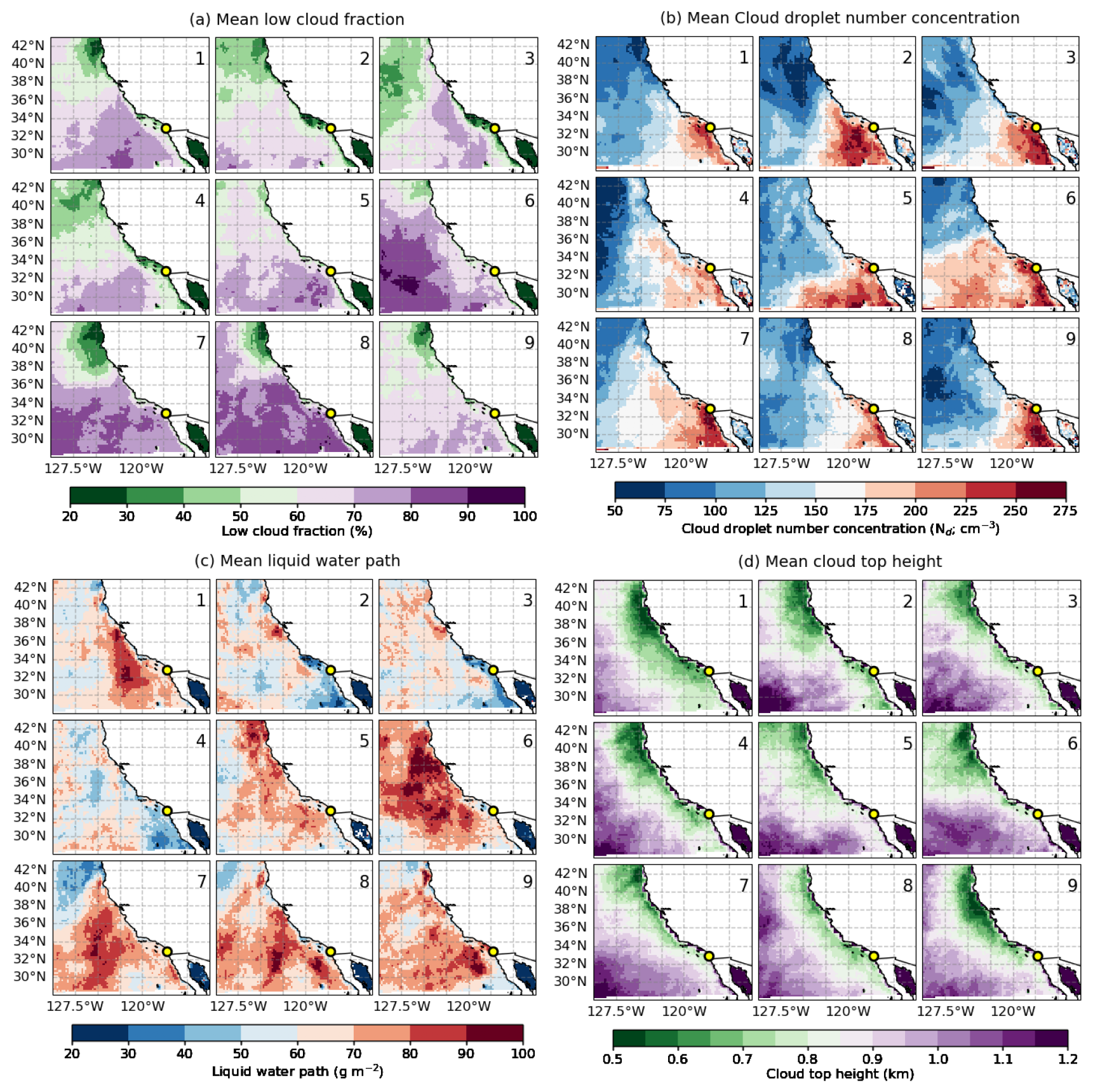
Figure 7 SatCORPS GOES-18 cloud properties composited across nine synoptic regimes for April to September 2023. (a) Low-cloud fraction, (b) cloud droplet number concentration, (c) liquid water path, (d) cloud top height, for the daytime warm boundary layer clouds with low cloud fraction > 10 %, cloud optical depth > 2, and LWP range 5–250 g m⁻². The yellow circle indicates the Scripps Pier site.

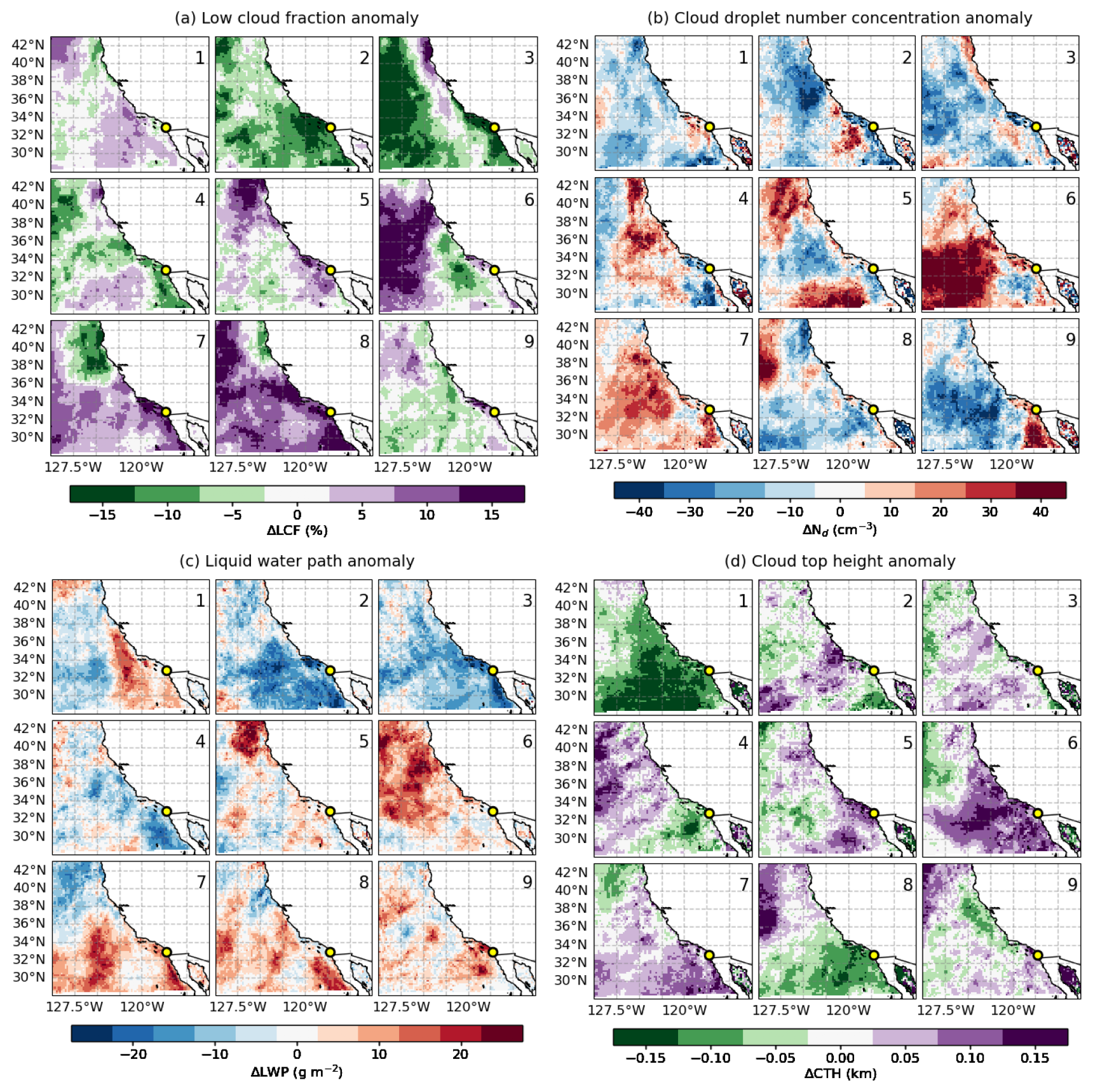
Figure 8 SatCORPS GOES-18 composite anomalies across nine synoptic regimes for April to September 2023. (a) Low-cloud fraction, (b) cloud droplet number concentration, (c) liquid water path, (d) cloud top height, for the daytime warm boundary layer clouds with low cloud fraction > 10 %, cloud optical depth > 2, and LWP range 5–250 g m⁻². The yellow circle indicates the Scripps Pier site. Anomalies are computed relative to the 30 d running mean climatology.

Figures 7b and 8b show the spatial mean and anomaly fields of SatCORPS GOES-18 N_d across the nine synoptic regimes. All regimes exhibit a strong coastal gradient in N_d with local maxima (> 200 cm⁻³) occurring nearshore and a systematically westward decrease. This well-known pattern is consistent with an expected continental aerosol outflow, dilution and precipitation scavenging offshore. Interestingly, under well-developed high-pressure conditions with stronger boundary layer winds (e.g., regimes 1–8 with the exception of regime 6), N_d enhancement is limited to a narrow coastal band and decreases abruptly to ∼ 100 cm⁻³ offshore. This suggests that intense anticyclonic circulations hinder the transport of continental aerosol over the open ocean, confining CCN sources to coastal regions. Notably, regime 6 features the largest extent of positive N_d anomalies and mean values greater than 175 cm⁻³, associated with a northwest displacement of the anticyclone and winds that run parallel to the coast north of 35° N. This unique synoptic configuration was also identified in Painemal et al. (2015) as the circulation that drives the highest N_d during MAGIC over the NEP.

The LWP variation in 9 synoptic regimes are featured in Figs. 7c and 8c. Broadly, the regimes of anomalous high-pressure areas around the coastal Southern California (e.g., regimes 2, 3, 4) with developing cyclone in the northwest relate well with the regimes of lower LWP below 60 g m⁻²along the coast, and anomalies reaching as much as 20 g m⁻² less than the mean climatology. These regimes are often characterized by shallower marine boundary layers with CTH below 800 m. Regimes 6–9 exhibit enhanced LWP frequently exceeding 75 g m⁻² across large spatial extents. These regimes also show strong positive LWP anomalies, in some cases surpassing 20 g m⁻² compared to climatological means. High values of LWP in these regimes appear to coincide with regimes of anomalous cyclone to the coast and a boundary layer deepening (Fig. 8d). Regionally, satellite CTH (Fig. 7d) shows shallower clouds along the coast (a region with cooler sea surface), with cloud top deepening farther offshore over warmer waters. Most synoptic regimes exhibit mean CTH values within 800 m along coastal California, except regimes 5–7, which reach ∼ 1 km. Deseasonalized CTH patterns highlight distinct variations: most anomalous anticyclone dominant regimes (1–4) display systematically lower cloud tops, while the other regimes except regime 8 show higher cloud tops, particularly over the Southern California.

3.5 Cloud characteristics from observations at Scripps Pier

Regime-specific comparison of SatCORPS satellite retrievals and EPCAPE ground-based observations of key cloud properties are shown in Fig. 9. The SatCORPS satellite data here correspond to the 0.2° grid box around Scripps Pier. Both GOES-18 and KAZR-derived CTHs exhibit similar variability across regimes however satellite derived CTHs shows consistently higher range up to an overestimate of ∼ 250 m. A key difference is the smaller lower quartile magnitude for the KAZR, likely attributed to the ability of the radar to detect small shallow cumulus clouds that are undetected at the satellite pixel resolution. Both the ground based and remotely derived CTH show the shallowest median cloud tops (< 1000 m) in regimes 1–4, where the anticyclone is centered closer to Scripps Pier, as indicated by positive SLP anomalies over the pier and adjacent land areas (Figs. 7d and 8d). In contrast, deeper cloud tops are observed in regimes with an anticyclone accompanied by a weak coastal low (regimes 5–8, Fig. 2a), reflected in negative anomalous SLP around Scripps Pier (Fig. 3a). To note, highest surface precipitation events were noticed in regimes 6 and 7 (0.45 % and 0.95 % occurrence frequency) although which is < 0.1 % occurrence frequency and the datasets are removed from the analysis. The ceilometer derived CBH in Fig. 9b shows that regime 6 often develops cloud bases closer to the surface (median ∼ 250 m), under the most stable boundary layer conditions (Fig. 6a). The mean ceilometer derived CBH in Fig. 9b is within 450 m in regimes with an anticyclone centered close to Scripps Pier (regimes 1–4). Regimes 5–8, on the other hand, show the highest mean cloud base (> 600 m) in accordance with increased TKE, deeper, and decoupled BL. Figure 9c shows LWP variation across the regimes from both the ground-based MWR and GOES-18 SatCORPS retrievals, both exhibit broadly consistent regime-to-regime variability except that the MWR LWPs are slightly higher. At the Scripps Pier site, regime 2, characterized by moderate synoptic forcing, shows the lowest mean LWP. Regimes 5–8 consistently exhibit reduced LWP, whereas the climatologically closer depicting regime 9 displays largest LWP.

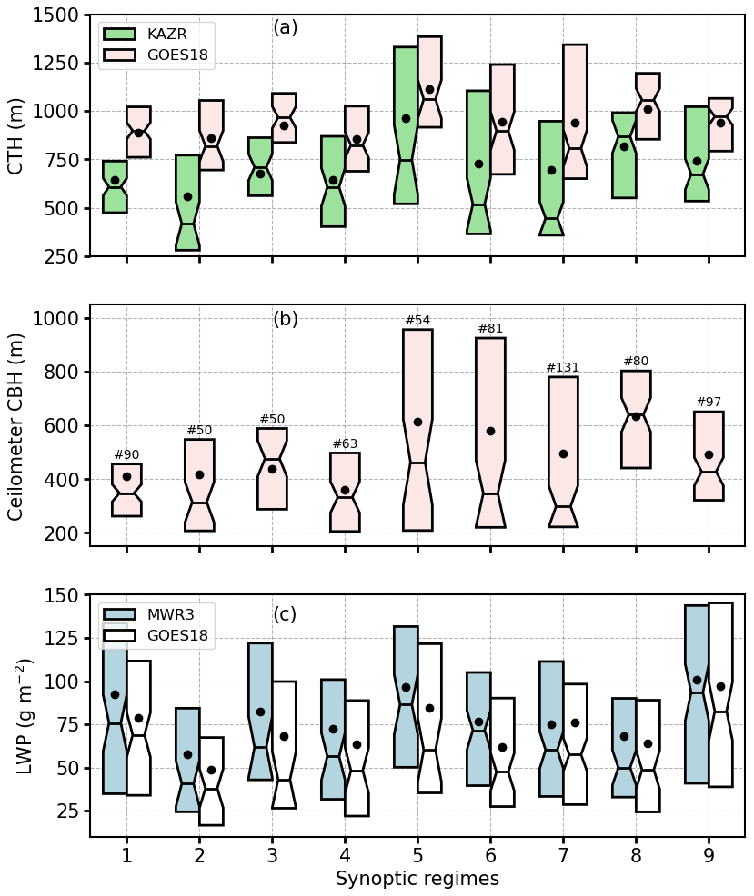
Figure 9 Comparisons of SatCORPS GOES-18 satellite vs. EPCAPE ground-based observations of (a) cloud top height, (b) cloud base height, and (c) liquid water path for the daytime, non-precipitating warm boundary layer clouds with hourly cloud frequency > 20 %, low cloud fraction > 10 %, cloud optical depth > 2, and LWP range 5–250 g m⁻². Notches represent the 95 % confidence interval of the median. The number of samples for each regime is shown in panel (b).

3.6 Aerosol and cloud droplet concentration at Scripps Pier

To assess how synoptic regimes modulate aerosol variability and transport at Scripps Pier, we analyze number concentrations of smaller particles (N_a ≤ 0.1 µm, N_a≤0.1) and larger accumulation-mode particles (0.1 < N_a < 1 µm; N_a>0.1), derived from merged SMPS and APS measurements (Fig. 10a). Smaller particles are typically associated with fresh local emissions and pollution, whereas larger particles reflect aging-driven growth or contributions from marine and continental sources such as sea spray or dust. Both size modes exhibit substantial variability across synoptic regimes. As inferred from Fig. 10a, upper quartile concentrations of N_a≤0.1 exceed 600 cm⁻³ for all the regimes, but with the lowest medians for regimes 6 and 9. While N_a>0.1 generally follow a similar regime evolution with the median values > 300 cm⁻³, regimes 3, 4, and 9 exhibit a narrow range of these particles. Overall, N_a≤0.1 are significantly higher than N_a>0.1 in most regimes.

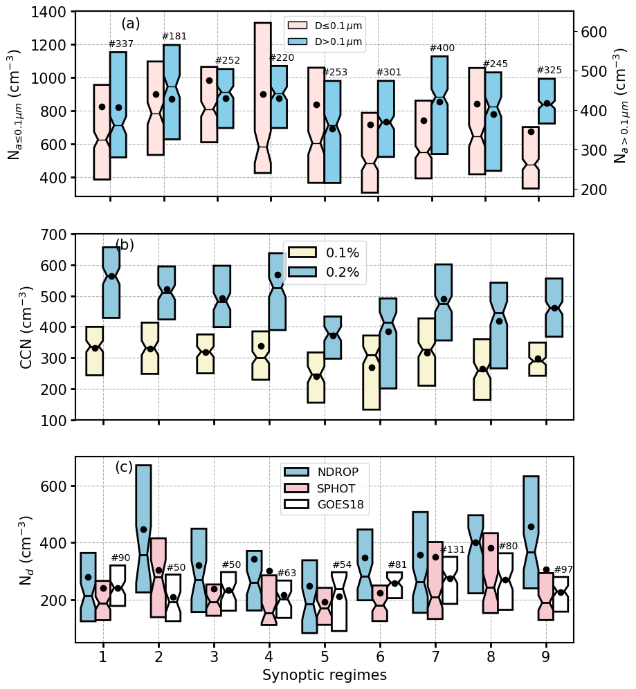
Figure 10 Boxplot of (a) aerosol number concentrations N_a (cm⁻³), (b) cloud condensation nuclei (cm⁻³), and (c) cloud droplet number concentration (cm⁻³) for nine synoptic regimes at Scripps Pier for April to September 2023 for the non-precipitating daytime conditions. Notches represent the 95 % confidence interval of the median. The number of samples for each regime is shown on the figure.

In terms of CCN at 0.2 % of supersaturation (CCN_0.2 %, Fig. 10b, blue), regime changes are somewhat similar to N_a>0.1, with concentrations comparable to those for N_a≤0.1. CCN at 0.1 % supersaturation (CCN_0.1 %) is, as expected, smaller than CCN_0.2 % but with qualitatively similar regime changes. The accumulation mode particle concentration N_a≤0.1 is higher than CCN concentrations at 0.1 % SS but lower than CCN concentrations at 0.2 % SS. This finding is consistent with Dedrick et al. (2026) that found SS below 0.2 % at Scripps Pier. Changes in CCN with supersaturation can be further analyzed in the context of clouds by examining variation in N_d derived from GOES-18 and from the remote sensors at the pier (Fig. 10c). N_d values are similar to the concentrations for CCN_0.1 %, suggesting small magnitudes of supersaturations present in this region, limiting the number of particles activated despite relatively large aerosol concentrations (Fig. 10a). Both satellite and the ground-based remote sensors show similar changes in N_d with regimes, but with larger interquartile ranges for the ground-based observations. The discrepancies between ground-based and GOES-18 N_d cannot be easily explained as we do not count on independent in-situ observations to validate these computations. Therefore, the data interpretation will be based on features common to both satellite and ground-based N_d. Regimes 2 as well as 6-8 consistently exhibit higher N_d with the mean N_d ranging ∼ 250–400 cm⁻³, whereas regimes 1, 3, 4, and 9 show lower mean N_d (∼ 200–250 cm⁻³). This variability in N_d aligns with TKE pattern in regimes (Fig. 6c); as regimes with stronger turbulence tend to exhibit higher N_d, even when particle number concentrations and CCN concentrations are comparable to, or lower than, those in the weekly turbulent regimes.

While aerosol loading is controlled by synoptic and local variability, N_d responses are likely influenced by BL turbulence and cloud dynamics. For assessing the impact of turbulence in aerosol and cloud droplet concentration, we bin N_d as function of accumulation mode N_a (N_a>0.1) and TKE bins (Fig. 11). As TKE increases from 0.1 to 0.5 m²s⁻², N_a>0.1 increase from 320 to 520 cm⁻³, suggesting that enhanced turbulence is associated with higher concentration of accumulation mode aerosols. In addition, we observe an increase of the ground-based N_d with TKE, with changes that exceed 200 cm⁻³, reinforcing the role of turbulence in strengthening aerosol activation into CCN. The averaged N_d as a function of TKE and N_a indicates that an increase in N_a combined with strong TKE leads to a higher N_d. It appears that the relationship between TKE and N_d are tighter, only when there is a sufficiently higher concentration of accumulation mode aerosol particles (N_a>0.1 >400 cm⁻³).

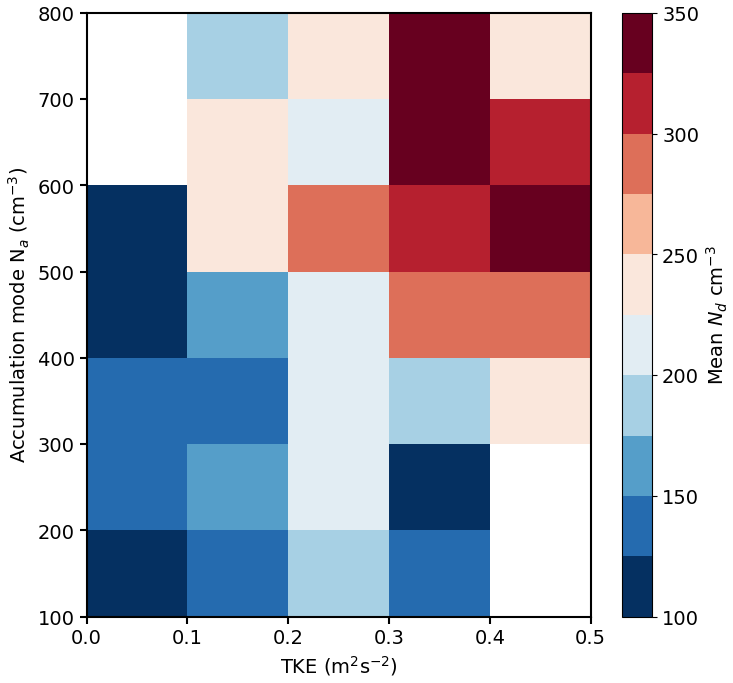
Figure 11 Relationship between turbulence kinetic energy, and, aerosol and cloud droplet number concentration depicted in a two-dimensional binning of N_d as a function of TKE and N_a for particle size range 0.1–1 µm.

Backtrajectories in Fig. 12 are dominated by a flow that runs parallel to the coast (Han et al., 2025; Maneenoi et al., 2025). A departure from this pattern is observed for regimes 1–3, which feature a significant number (> 30 %) of trajectories that originate from or intersect land areas. Given the modest changes in the backtrajectory pattern per regime, it is not possible to establish a relationship between long-range transport, backtrajectories, and aerosol variability. This suggests that for this coastal site, local aerosol sources and transport (e.g., land-sea breeze), are, at least, as important as the synoptic meteorology for explaining aerosol variability. In terms of aerosol composition, non-refractive organics is the dominant species at Scripps Pier, followed by sulfate and ammonium (Fig. 13). A synoptic-scale maximum in all species (organics, sulphate, Ammonium and Nitrate) is identified for regime 4. Regimes 3 and 5 exhibit a minimum in organics. With greater percentage of land intersecting trajectories, regime 2 depict higher concentration of organics, however, the species concentrations are non-correlative nature to the land intersecting trajectories likely due to the seasonally dominant marine sources of these species.

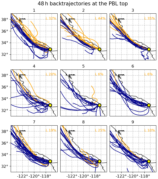
Figure 12 ARMTRAJ-PBL airmass backtrajectories initiated at Scripps Pier (yellow circle) at PBL top for the nine synoptic regimes labelled from 1 to 9. Trajectories from or crossed over land are shown in orange color, and the corresponding percentage of trajectories for each regime is shown on the figure.

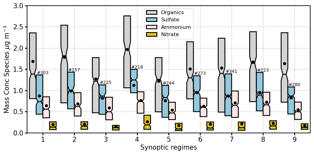
Figure 13 Mass concentration of aerosol composition at Scripps Pier for April to September 2023 non-precipitating daytime conditions for Organics (gray), sulfate (blue), ammonium (pink), and Nitrate (gold). Notches (sometimes negligible) represent the 95 % confidence interval of the median. The number of samples for each regime is shown on the figure.

4 Summary and discussions

We classified the atmospheric circulation over the northeast Pacific coastal region using Self-Organizing Maps, with the goal of understanding how synoptic variability modulates changes in aerosol and cloud characteristics. Detailed MBL and local cloud and aerosol observations were provided by the ARM for the ground-based site at Scripps Pier in Southern California and GOES-18 satellite cloud products from SatCORPS during the ARM DOE Eastern Pacific Cloud Aerosol Precipitation Experiment (EPCAPE) campaign. We identify nine synoptic regimes, representing dominant meteorological patterns influencing coastal Southern California during April through September 2023. The regimes can be interpreted in terms of the anticyclone/cyclone evolution as follows: regime 1 captures the broadest spatial development of the high pressure, with ubiquitous subsidence. Regime 2 features a relatively well-developed anticyclone at the center of the domain, with a cyclonic development at the northwestern edge of the NEP. The cyclone migrates southward, confining the anticyclone south of 35° N in regimes 3 and 4. This cyclone reaches its maximum southward extent for regime 5, featuring upward motions that are typical of midlatitude storms, conditions often associated with heavy precipitation episodes (Neiburger et al., 1961; Gershunov et al., 2019). As the low pressure moves eastward over land in regime 6, a new migrating anticyclone moves to the northwest, with strengthening and eastward displacement in regimes 7 and 8. Regime 9 represents conditions that minimal depart from the climatological mean.

MBL structure exhibits pronounced regime-dependent variability, reflecting contrasts in stability, humidity, and circulation. Regimes 1–4, with an anomalous anticyclone closer to Scripps Pier, are characterized by a shallower boundary layer, weaker turbulence, and coupled MBL. In contrast, regimes 5–8, with an anomalous cyclone closer to Scripps Pier and a well-developed anticyclone core (particularly for regimes 6–8) north of Scripps Pier, feature a deeper boundary layer, weaker MBL static stability, with regime 7 possessing the highest mean TKE. Generally speaking, stable boundary layers are associated with the presence of shallow boundary layer (regimes 1–4), while the reduced stability in regimes 5–8 support deeper, more turbulent layers, which are conditions typically associated with transition toward shallow cumulus convection (Teixeira et al., 2011; Zhou et al., 2015; Bretherton and Blossey, 2017). Zonal winds are modest westerlies (< 4 m s⁻¹), whereas meridional winds are predominantly northerlies in all regimes but shifts to southerlies in regimes 7 and 8, favoring advection of warm moist air from the south and resulting in increased clouds and precipitation. Regime 9 which most closely resembles the climatological mean pattern, exhibit MBL characteristics intermediate between those of the stable regimes (1–4) and the more turbulent, less stable regimes 5–8.

The regional analysis of SatCORPS GOES-18 regime composites of LCF, N_d, LWP, and CTH reveal the influence of synoptic-scale meteorology on low-level clouds along the Southern California coast. Across all regimes, cloud cover remains high off the California coast, generally exceeding 70 % off California coast. Synoptic regimes characterized by an anticyclone centered near 30–35° N and positioned closer to coastal Southern California (regimes 1–4) exhibit slightly reduced low-cloud amount (LCF < 50 %) and negative anomalies (−5 % to −15 %) along the shoreline. In these regimes, the spatial pattern of LWP closely mirrors the reduction in LCF, and CTHs remain shallower. Conversely, a northwest displacement of the anticyclone and a weak low-pressure pattern inland (regimes 7–8) appear to support extensive stratocumulus (LCF > 75 %) and positive LCF anomalies (∼ 15 %) under weaker subsidence along the coast. Regimes 7 and 8 also feature a boundary layer deepening (CTH > 1 km) and a consistent increase in LWP. N_d exhibits strong coastal gradients for all regimes, exceeding 200 cm⁻³ nearshore and decreasing offshore, consistent with continental aerosol outflow and more active precipitation scavenging farther offshore (e.g. Wood et al., 2012). Wind strengthening and a flow that runs parallel to the coastline for all the synoptic regimes appear to confine aerosol advection to a narrow coastal band, resulting in a drastic decrease in N_d of 100 cm⁻³ just 5° degrees west from Baja California (30° N, 115° W), except that the regimes 6 and 7 show wider area of greater N_d and positive N_d anomalies (> 20 cm⁻³).

Comparisons between SatCORPS satellite derived and EPCAPE ground-based radar observations at Scripps Pier show that the satellite CTH are higher (∼ 250 m) than the ground based radar measurements. The radar can detect small shallow clouds typically well below the inversion, which are too small to be resolved at the satellite pixel resolution, which causes satellites to report slightly higher cloud tops. Additionally, GOES-18 cloud-top height retrievals can be challenging along the shoreline boundaries due to issues with surface temperature. Satellite and the ground-based microwave LWP agrees within 5–20 g m⁻², with ground-based LWP being always higher. N_d derived from ground-based cloud-mode sun photometer derived cloud optical depth and microwave radiometer derived LWP, NDROP N_d (N_d derived from MFRSR derived cloud optical depth and microwave radiometer derived LWP; Zhang, 2023), and satellite retrievals show considerable variation in range but similar pattern in variation for the synoptic regimes, though the NDROP N_d are systematically higher (Fig. 3a, Sorooshian et al., 2019). This N_d comparison also highlights the challenges of indirectly deriving N_d with remote sensing observations (e.g., Grosvenor et al., 2018). While N_d estimated from GOES-18 has the advantage of being derived with retrievals from a radiometrically consistent algorithm, the coarse pixel resolution (2 km) prevents the detection of small clouds. While ground-based retrievals are in principle more accurate, the need of combining data from 2 different instruments (microwave and visible radiometers) could result in significant noise in the estimated N_d, especially when biases in LWP or cloud optical depth are not properly characterized. Even though retrievals of cloud droplet effective radius are available from the sun-photometer and the multifilter rotating shadowband radiometer, the derivation of r_e from ground-based passive radiometers is more prone to uncertainties than cloud optical depth (e.g. Chiu et al., 2012). Given how critical N_d is for understanding aerosol effects on clouds, future field deployments would benefit from dedicated efforts of intercomparing and evaluating N_d products, especially when in-situ cloud microphysical observations are available.

Analysis of particle number concentrations at Scripps Pier reveals that the regime classification does not result in evident aerosol changes, possibly because the site is near multiple local pollution sources, while winds modestly change at the site during the period of study. Indeed, backtrajectories reveal predominantly coastal-parallel flow, with regime 1–3 featuring land influence, but minimal trajectory variability, suggesting that local sources and mesoscale processes are important for understanding aerosol variability (e.g., land–sea breeze).

CCN concentration at 0.2 % supersaturation mirrors the changes in accumulation mode particle concentration, whereas CCN at 0.1 % more closely matches the N_d values. These findings aligns with the low values of supersaturation over the coastal region (Dedrick et al., 2026), and how this environmental constraint prevents more aerosols from being activated into droplets despite high aerosol concentrations. For instance, the highest TKE value for regimes 7–8 are concomitant with high mean N_d and the N_d highest upper quartile. Conversely, the lower N_d in regimes 1–4, despite having slightly higher concentrations of CCN and accumulation mode aerosols, appears to be partially explained by the low turbulence for these regimes. In a broader sense, the N_d variability shown in Fig. 11, reflects the combined influence of accumulation mode aerosol concentration and boundary layer turbulence, with the highest N_d occurring under conditions of both elevated accumulation mode concentrations and enhanced TKE, which are two primary factors governing droplet formation. The analysis also suggests that due to weak values of supersaturations, a relatively small fraction of large mode aerosols (accumulation mode) is activated for concentrations smaller than 600 cm⁻³, especially when the turbulence is modest. It follows that detailed information of updraft velocity and supersaturations are essential for understanding observational regressions between N_a–N_d, metric commonly referred to as the aerosol-cloud interactions (ACI) metric (Bellouin et al., 2020). Another factor not investigated in this study is the role of precipitation, as drizzle and occasional surface precipitation in subtropical stratiform regimes (Wood, 2005), can further reduce N_a through coalescence scavenging and wet deposition, in turn, impact ACI metrics. A more detailed assessment will be conducted in future work by combining ARM observations to better characterize drizzle occurrence and quantify its relevance for aerosol scavenging and ACI behavior. Because specific meteorological regimes feature unique characteristics in terms of inversion strength, boundary layer deepening, and turbulence, the classification proposed here offers an alternative approach to the problem of disentangling the meteorological control over N_d variability, which is critical for understanding how aerosols impact clouds in the context of the aerosol indirect effect.