Classification and quantification of low-visibility events using deep learning over eastern China

Low-visibility events (LVEs) threaten transportation safety and human health, yet accurately identifying them at a regional scale remains challenging. To address this, this study introduces a unified convolutional neural network (CNN) framework that integrates the geostationary satellite, meteorology, and fine particulate matter (PM_2.5) observation data to identify all types of LVEs. The model can not only produce the spatiotemporal distribution of LVEs, including land and sea fog, but also quantify the intensity of LVEs linked to visibility reduction. By incorporating PM_2.5, the polluted fog-haze over land can be discriminated from clean fog. Based on the model, we are able to investigate the environmental policy to reduce fog-haze and the corresponding population exposure. Over eastern China, a 20 % reduction of overall PM_2.5 can reduce the fog-haze area by 43 % in winter. However, the corresponding population exposure is reduced less effectively by 15 %, because the most populated region collocates with the most polluted region, where a further reduction of PM_2.5 by over 40 % is required to effectively reduce its population exposure. Here, the classified and quantified LVEs, along with the established relationship with pollution, explicitly guide the air-quality policy for the co-benefits of improving air visibility and human health.

1 Introduction

Low-visibility events (LVEs) occur across both terrestrial and marine environments. LVEs are defined by reduced near-surface visibility and can be associated with fog, haze, fog-haze mixtures, drizzle, rain, snow, ice fog, and other mixed hydrometeor conditions (Gultepe et al., 2007b, 2015, 2019). The weather records are analyzed from 2412 stations in February (Fig. S6a in the Supplement), showing fog contributed to 73 % and 59 % of weather types for inland and coastal sites, respectively. Rain contributed to the second important weather types, with 18 % and 17 % for inland and coastal sites, while the others are <5 %. The classified fog in this study therefore may contain some precipitation, but has not been further separated. LVEs degrade atmospheric transparency through light extinction by suspended liquid droplets and aerosol particles. Fog forms when near-surface air becomes sufficiently saturated for aerosols to activate into cloud droplets (Gultepe et al., 2007b). The microphysical properties of droplets, including the size spectrum and relative dispersion, can be influenced by aerosol concentration (Twomey, 1977; Liu and Daum, 2002). The amount of aerosols contained in fogs can also determine the pollution level of fogs, as a polluted fog containing high aerosol loadings (i.e., the fog-haze) can exert adverse health impacts (Zhang et al., 2014). Identifying different types of LVEs is important to understand their impacts and to make effective environmental policies.

Satellite remote sensing provides a powerful tool to identify fogs from complex cloud types on a broad spatial scale (Gultepe et al., 2007a; Cermak and Bendix, 2008). The use of satellite observations for fog detection is often limited by the absence of visible channels at night and by contamination from mid- and high-level clouds. Traditional fog identification relies on fixed thresholds applied to one or more parameters, which can be difficult to generalize across changing surface and cloud conditions (Ellrod, 1995; Eyre et al., 1984; Gultepe et al., 2007a). For instance, nighttime fog is typically detected utilizing the brightness temperature difference (BTD) between infrared channels (Eyre et al., 1984; Hunt, 1973). For daytime detection, the algorithm utilizes visible and 3.9 µm shortwave infrared reflectance to distinguish water clouds from snow and ice (Lee et al., 1997; Anthis and Cracknell, 1999). Additionally, textural thresholds distinguish smooth fog from rough clouds (Wu et al., 2015), and the temperature difference between the cloud top and sea surface confirms low-level fog (Zhang and Yi, 2013). By contrast, machine-learning and deep-learning methods can learn nonlinear relationships among multiple variables and may improve detection performance compared with fixed-threshold methods (Shin and Kim, 2018; Jeon et al., 2020; Huang et al., 2022). Model generalization can also benefit from the integration of large-scale multi-source data (Xu et al., 2025). Satellite spectral data capture cloud and aerosol signatures, meteorological reanalysis describes fog-favorable conditions, and ground-based PM_2.5 indicates aerosol loading. Together, these inputs help distinguish clean fog from polluted fog-haze, which can resemble cloud in satellite imagery (Hutchison et al., 2008). Furthermore, regarding the distinction between polluted and unpolluted fog, although studies have noted microphysical differences, including a smaller droplet effective radius in polluted environments (Mazoyer et al., 2019), operational methods to explicitly identify the polluted fogs remain scarce. Given these detection challenges, only a limited number of studies have addressed the broader range of LVE types, including land and sea fog, unpolluted and polluted fog, and other mixed hydrometeor conditions, thereby examining their interactions and transitions (Gultepe et al., 2007b, 2015, 2019).

In this study, we develop a multi-source fusion model based on a convolutional neural network (CNN) to identify all types of LVEs over land and sea. This model integrates the satellite spectral data with the meteorology reanalysis and ground PM_2.5 observations. By systematically altering PM_2.5 concentrations in the model, we quantify the impact of pollution abatement on winter fog-haze to guide the cost-effective air quality policy.

2 Data and observations

2.1 Study region

The study focuses on eastern China (Fig. S1 in the Supplement), a region characterized by a monsoon climate, dense population, and intense anthropogenic emissions (Zhang et al., 2009; Li et al., 2017). This region frequently experiences interactions between marine moisture and anthropogenic aerosols, generating all types of LVEs, including land and sea fog as well as polluted and unpolluted fog (Niu et al., 2010).

2.2 Multi-source observational datasets

We constructed a multisource dataset for 2019–2020 by integrating geostationary satellite observations, meteorological reanalysis, air quality measurements, and ground-based visibility observations (Table S1 in the Supplement). Satellite inputs were obtained from FY-4A and included brightness temperatures (BT) at 3.72 and 10.8 µm, together with solar zenith angle (SOZ) (Yang et al., 2017). The 10.8 µm thermal infrared channel provides information on cloud top temperature, effectively separating low-level fog from colder, elevated cloud layers (Cermak and Bendix, 2008). The 3.72 µm shortwave infrared channel distinguishes fine haze from fog, as only the larger fog droplets trigger strong Mie scattering, while haze interacts weakly (Gultepe et al., 2007b). The brightness temperature difference between these two channels (BTD, BT_3.72−BT_10.8) enhances the spectral contrast among fog, haze, and the background (Hunt, 1973). Solar zenith angle was included to account for variations in illumination during the diurnal cycle (Wei et al., 2021).

Meteorological variables were obtained from ERA5 reanalysis, including 2 m temperature and 2 m dew point temperature (Hersbach et al., 2020). The temperature and dew point spread was used as a proxy for near-surface saturation and helped distinguish ground-contacting fog from unsaturated low stratus or aerosol dominated haze (Pauli et al., 2020). Hourly PM_2.5 concentrations were obtained from the China National Environmental Monitoring Centre (CNEMC) and used to represent aerosol loading over land. Hourly ground-based visibility observations were obtained from the NOAA/NCDC Integrated Surface Database Lite (ISD-Lite) and used as the observational basis for LVE labelling. Population data at 1 km resolution were obtained from WorldPop and used only for the population exposure analysis. The temporal matching, spatial collocation, and uncertainty evaluation of these multi-source datasets are described in Sect. 2.4 and Text S1 in the Supplement.

2.3 Visibility definition and LVE labelling

In this study, visibility (Vis) refers to the near-surface horizontal meteorological optical range, namely the distance over which the contrast of an object against the background is reduced to a threshold perceptible to a human observer (WMO, 2025). Figure S6a shows the near-surface low visibility is governed primarily by fog droplets, aerosol particles, and other hydrometeors. Following the Koschmieder relationship, Vis can be related to the atmospheric extinction coefficient β_ext as $\text{Vis}=\mathrm{3.912}/{\mathit{\beta }}_{\text{ext}}$ (Israël and Kasten, 1959). Therefore, a reduction in Vis indicates enhanced near-surface optical extinction.

The occurrence of LVEs was defined using ground-measured visibility. Station observations with Vis≦2 km were labelled as low visibility, while observations with Vis>2 km were labelled as clear (Lyu et al., 2021). The station-level labels were then mapped to the nearest 4 km FY-4A grid cell to generate a binary mask for model training and validation. The CNN was trained on this binary mask to detect low visibility, while event types were assigned after prediction using temperature-dew-point spread and PM_2.5 (Sect. 3.1).

2.4 Data collocation and preprocessing

All datasets were temporally matched to the hourly visibility observations and spatially resampled to the 4 km FY-4A grid. All times are given in local time (LT, UTC+8). ERA5 variables and station-based PM_2.5 and visibility observations were interpolated or assigned to the satellite grid, and missing values were filled using nearest-neighbour interpolation. The collocated variables were then cropped into 64×64 pixel windows for CNN training and prediction, as illustrated in Fig. 1. The collocated variables were retained as fixed-size 64×64 tensors on the FY-4A grid, rather than being averaged across regions with different pixel numbers. Because the datasets differ in spatial resolution, sampling frequency, and measurement height, this collocation may introduce representativeness uncertainty. We therefore quantified the station-to-grid uncertainty using nearest-station distance statistics and leave-one-out cross-validation for PM_2.5 and visibility labels (Fig. S2 in the Supplement). Further details of data preprocessing, standardization, and uncertainty evaluation are provided in Text S1.

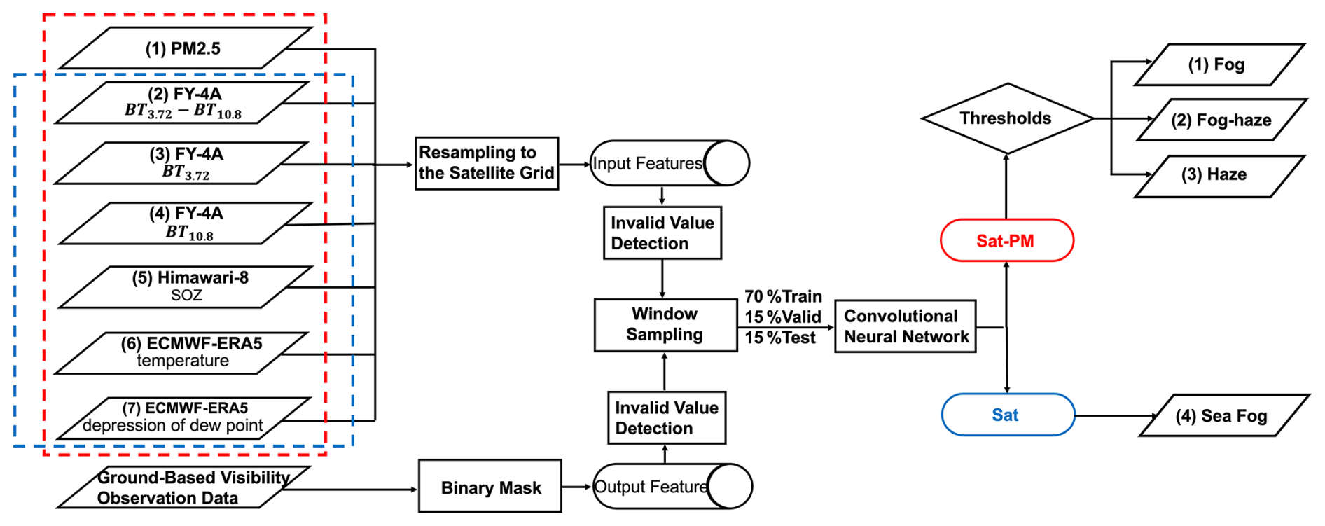
Figure 1 Schematic of the analytical framework. The blocks from left to right are the input and output parameters, the procedures of dataset preparation for the machine learning, and the model outputs. The ground visibility observations are processed into a binary mask to serve as the output for model training. The framework utilizes the convolutional neural network (CNN) to output the map of low-visibility events over land, including fog, fog-haze, and haze, using satellite, meteorological and PM_2.5 data (the Sat-PM model), and sea fog using satellite and meteorological data (the Sat model).

3 Methodology

3.1 Overall framework and physical attribution

The overall framework for identifying and attributing low-visibility events (LVEs) is illustrated in Fig. 1. Ground-based visibility observations were used to generate the binary low-visibility mask for model training. Multisource satellite, meteorological, and PM_2.5 fields were collocated on the FY-4A grid and processed using a window-sampling strategy. The CNN first identifies low-visibility pixels through binary classification against clear conditions. These pixels are then assigned to individual LVE types using physically interpretable environmental criteria.

Over land, identified low-visibility pixels were attributed using dew point depression as a proxy for near-surface saturation and PM_2.5 as a proxy for aerosol loading. Pixels were classified as fog when dew point depression was <3 °C and PM_2.5 was <75 µg m⁻³, as fog-haze when dew point depression was <3 °C and PM_2.5 was ≥75 µg m⁻³, and as haze when dew point depression was ≥3 °C and PM_2.5 was ≥75 µg m⁻³. This PM_2.5-based separation is to identify polluted fogs, rather than a microphysical definition of fog formation. In particular, the fog-haze category represents water-saturated, fog-favorable conditions under higher aerosol loading, to denote the fog occurring under higher aerosol conditions. The humidity criterion reflects fog-favourable near-surface saturation (Pauli et al., 2020), while the PM_2.5 threshold follows the Grade-II 24 h limit of the Chinese Ambient Air Quality Standard (GB 3095-2012; Ministry of Environmental Protection of the People's Republic of China and General Administration of Quality Supervision, Inspection and Quarantine of the People's Republic of China, 2012). Over ocean grids, low-visibility pixels from the Sat model were attributed to sea fog. This post-processing scheme separates the optical occurrence of low visibility from its likely physical cause. Consistent with the operational definition in Sect. 2.3, we did not further subdivide LVEs by precipitation occurrence, because drizzle, weak precipitation, and fog often co-occur and rain-only cases generally do not represent the LVEs targeted here (Wang et al., 2021).

3.2 Model configuration to classify LVEs

The identification framework employs a CNN architecture to map the multi-source input tensors (dimensions of $C\times \mathrm{64}\times \mathrm{64}$, where C represents variable channels) to event probabilities. As detailed in Fig. S3 and Text S2 in the Supplement, the feature extraction module consists of three sequential convolutional blocks. Each block comprises a 3×3 convolutional layer to capture local spectral-spatial patterns, followed by batch normalization (BatchNorm) (Ioffe and Szegedy, 2015) and rectified linear unit (ReLU) activation (Krizhevsky et al., 2012) to ensure training stability. A max-pooling layer concludes each block, progressively reducing spatial resolution from 64×64 to 8×8 while expanding feature depth from 32 to 128 channels. The high-dimensional features are subsequently flattened and processed by two fully connected layers, reducing dimensionality from 8192 to 512, before the final Softmax activation yields the probability scores for low-visibility and clear classes.

To address the feature redundancy inherent in multi-source data and the spatial heterogeneity of the background, a dual-branch attention mechanism is embedded within the convolutional blocks. The variable-wise attention module utilizes global average pooling to compute importance weights for each input channel, allowing the model to adaptively prioritize the most informative channels while suppressing noise (Hu et al., 2018). The spatial attention module uses average pooling together with max pooling within each 64×64 input tensor, followed by a 7×7 convolution kernel to focus on informative regions, effectively distinguishing fog boundaries from complex underlying surfaces (Woo et al., 2018). In both branches, pooling is used only inside the attention module to derive attention weights and does not replace the spatial input or average across different regions.

Training is driven by a hybrid loss function designed to overcome the class imbalance between rare LVEs and frequent clear conditions. This function combines balanced focal loss and dice loss with equal weighting (Lin et al., 2017; Milletari et al., 2016). The focal loss down-weights easy negatives by setting a focusing parameter γ=3.0 and a balancing coefficient β=0.55, forcing the model to concentrate on minority samples. Meanwhile, the dice loss optimizes the F1-score, balancing precision and recall to ensure identification performance even when low visibility samples are rare. Detailed mathematical formulations and tensor transformations are provided in Texts S2 and S3 in the Supplement.

3.3 Model training and validation

The final dataset comprises 1440 LVEs observed during 2019–2020. A partition-then-sample strategy is introduced to divide events into training (70 %), validation (15 %), and test (15 %) subsets, followed by spatial samples extraction using non-overlapping sliding windows (142 km×142 km) as shown in Fig. S1b. Using ground-based observations as the ground truth, two model variants were trained: the land-based Sat-PM model, which incorporates PM_2.5 concentrations to separate clean from polluted low-visibility events, and the maritime Sat model, which excludes this input due to minimal anthropogenic influence over open oceans. The models were optimized using the AdamW algorithm with dynamic learning rate scheduling and early stopping mechanisms to ensure stable convergence. Furthermore, a progressive dropout strategy was applied to the fully connected layers to enhance generalization and prevent overfitting. Detailed training hyperparameters and regularization strategies are documented in Text S4 in the Supplement.

3.4 Metrics to quantify LVEs

Three parameters are defined to analyze the model outputs. The LVE intensity (I_pixel) is quantified using an overlapping sliding window approach (64×64 pixels with a stride of 8) that traverses the target area. Within each window, the model outputs a binary classification (low-visibility = 1 or clear = 0). The final intensity for a given pixel is defined as the ratio of positive classifications to the total number of overlapping windows covering that pixel. This can be expressed as:

$$\begin{array}{}\text{(1)}& I_{\text{pixel}}={\displaystyle \frac{{\sum }_{i=\mathrm{1}}^N{C}_i}{N_{\text{total}}}}\end{array}$$

where I_pixel denotes pixel intensity, N_total is the overlapping window count, and C_i indicates the ith window status (low-visibility=1 or clear=0).

The LVE area is calculated to characterize the spatial extent of events. This is derived by aggregating all grid pixels identified with positive LVE intensities (I_pixel>0) and converting the pixel count into geographical area (km²) based on the grid resolution.

The population-weighted intensity (PWI), referred to as population exposure, quantifies the average fog-haze intensity experienced by an individual within the study region. The gridded population distribution data were obtained from WorldPop (https://www.worldpop.org/, last access: 21 October 2026) at a resolution of 1 km. It is calculated by multiplying the fog-haze intensity in each grid cell (I_i) by the population in that cell (P_i), summing all grids over the entire domain, then dividing by the total domain population, as shown in Eq. (2):

$$\begin{array}{}\text{(2)}& \text{PWI}={\displaystyle \frac{{\sum }_{i=\mathrm{1}}^N(I_i\times P_i)}{{\sum }_{i=\mathrm{1}}^N{P}_i}}\end{array}$$

where i is an individual grid cell in the domain, N is the total number of grid cells, I_i is the fog-haze intensity in grid cell i, and P_i is the population in grid cell i.

4 Results

4.1 Overall performance of models

As summarized in Table S2 in the Supplement, the terrestrial Sat-PM model demonstrated superior performance on independent test datasets, achieving an overall accuracy of 0.93, an F1-score of 0.78, and a recall of 0.81. This accuracy reflects the binary classification of low-visibility versus clear conditions, whereas the correlation between modelled LVE intensity and observed visibility is evaluated in Figs. S6 and S7 in the Supplement. Individual LVE types are assigned through the physical attribution described in Sect. 3.1 rather than directly classified by the CNN. In parallel, the maritime Sat model proved robust for sea fog detection, securing an accuracy of 0.91 and a fog-specific F1-score of 0.71. Tables S3 and S4 in the Supplement provide the input-ablation and architecture comparisons, respectively.

4.2 Spatiotemporal distribution and intensity of classified LVEs

Figure 2a shows the input features for LVEs on 5–6 February 2019. The Sat-PM model is delineated by the red box, and the Sat model (blue box) operates without PM_2.5 data. A binary mask derived from ground-based station visibility observations serves as the ground truth (Fig. 2b), where red pixels denote areas classified as low-visibility (visibility≤2 km). The model output in Fig. 2c was subsequently assigned to different LVE categories using the two-step attribution scheme.

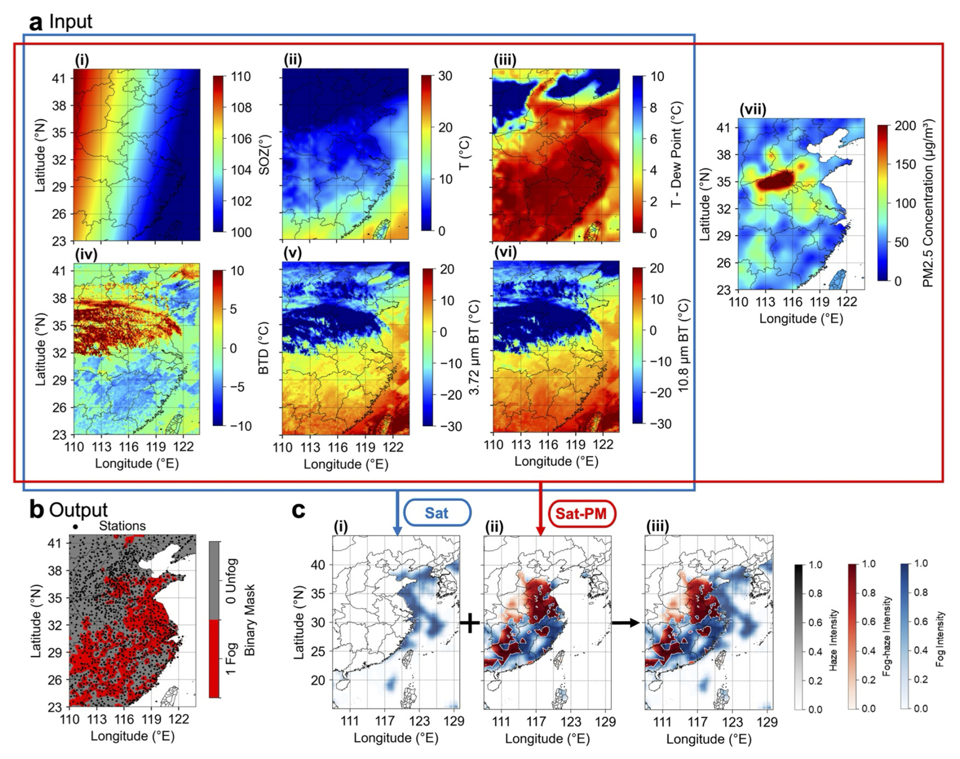
Figure 2 An example of input and output parameters to classify the spatial distribution of low-visibility events. (a) Input parameters, including solar zenith angle (i), temperature (ii), dew point depression (iii), brightness temperature difference (BTD) (iv), brightness temperature (BT) at 3.72 µm (v), BT at 10.8 µm (vi), and PM_2.5 (vii), are used for the Sat-PM model. (b) The binary mask determined by the ground observation of visibility, with red pixels representing low-visibility conditions (value=1). (c) The intensity maps of identified sea fog by the Sat model (i), fog and fog-haze by the Sat-PM model (ii), and combined results (iii).

Following the physical attribution scheme described in Sect. 3.1, the Sat model identifies sea fog over ocean grids (Fig. 2c(i)), while the Sat-PM model attributes terrestrial low-visibility pixels to fog, fog-haze, or haze (Fig. 2c(ii)). By integrating the outputs, a synthesized map (Fig. 2c(iii)) provides a comprehensive product that covers both land and sea. In the visualization, color opacity maps directly to the intensity of each phenomenon.

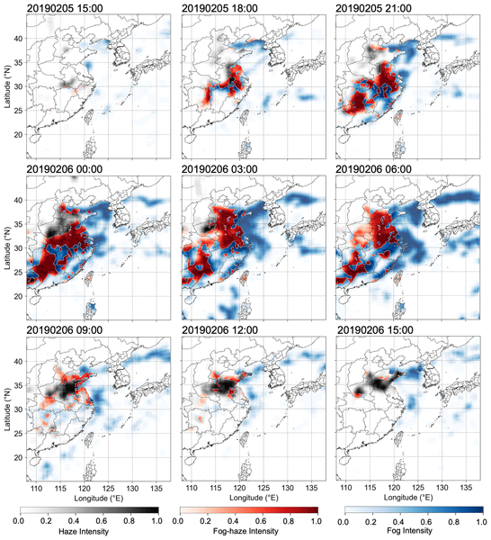
Figure 3 illustrates the spatiotemporal evolution of the LVE from 15:00 LT on 5 February to 15:00 LT on 6 February 2019. This case was selected because it captures co-occurring terrestrial and marine LVEs. The model results show that the low-visibility region initially formed along the coast and subsequently expanded inland and over the sea, intensifying and reaching its peak extent during the night and early morning. Thereafter, the low-visibility region gradually dissipated.

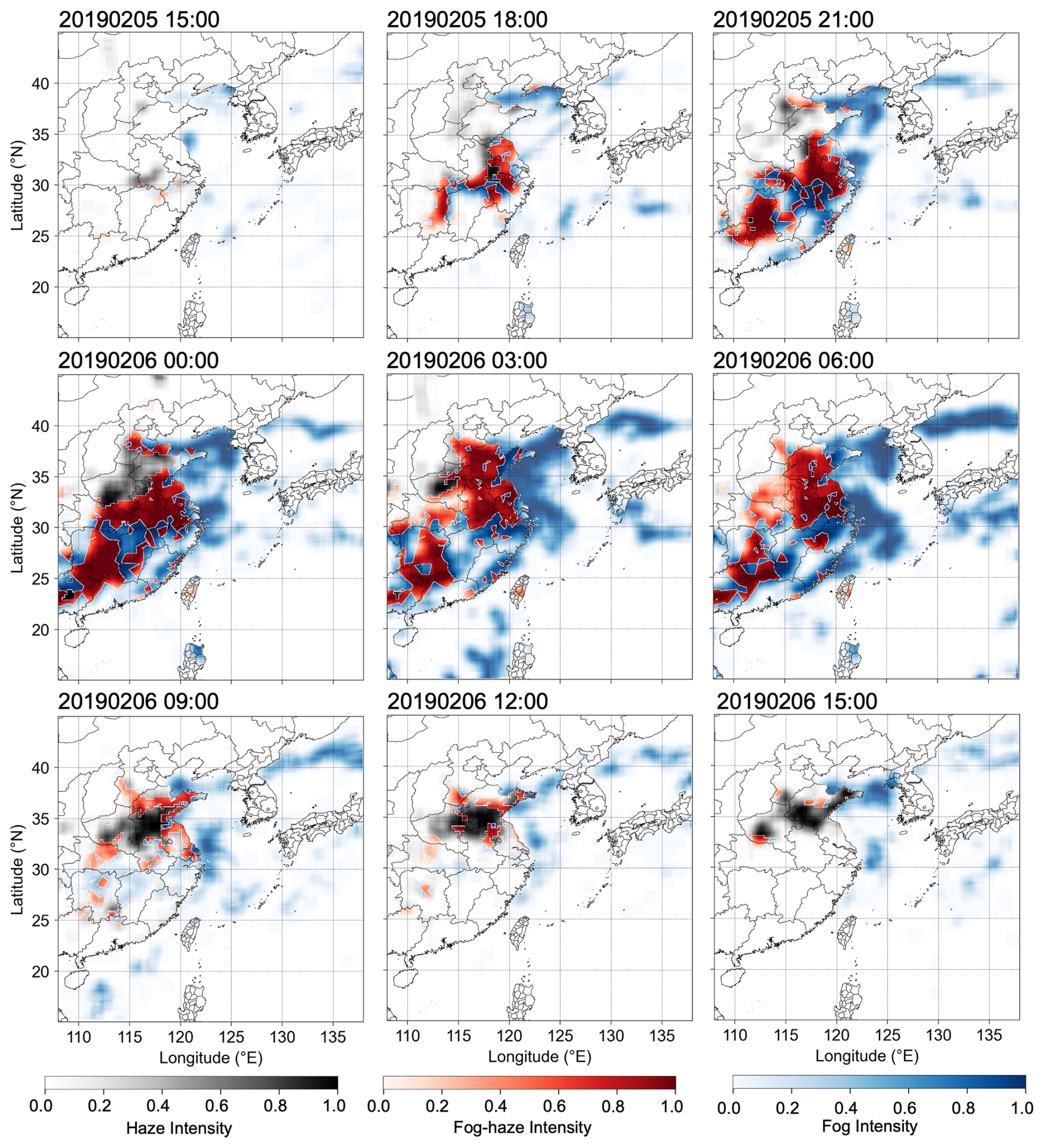
Figure 3 An example of the spatial distribution of low-visibility events with identified fog, fog-haze, haze and sea fog from 5 to 6 February 2019, all coloured by the intensity of classified events. All times in the figure and its caption are given in local time (LT, UTC+8).

To further evaluate model performance, we compared the simulated LVE intensity with ground-station visibility observations. The 15 February 2020 case was selected because continuous observations were available at both coastal and inland stations. Figure 4a shows the spatiotemporal evolution of a representative fog event on 15 February 2020, together with the locations of the validation stations. The model captures the main evolution of the fog, although some local mismatches are expected because of the uncertainty in model spatial resolution. Figure 4b(i) and (ii) show the temporal evolution at representative sea-fog and land-fog stations, respectively. At both coastal and inland sites, the simulated intensity generally follows the observed visibility reduction. The model curves in Fig. 4b(i) and (ii) are the arithmetic means of the model intensities extracted from the FY-4A grid cells nearest to the corresponding three sea fog and land fog stations, respectively. They provide regional summaries rather than intensities for individual stations. Separate station comparisons are provided in Figs. S8 and S9 in the Supplement, respectively. The correlations between model-derived fog intensity and observed visibility reduction (5 km – Vis) are shown for 821 validation stations in Fig. S6b and c, showing 62 % of the stations have r>0.6, validating the model performance to predict LVE intensity.

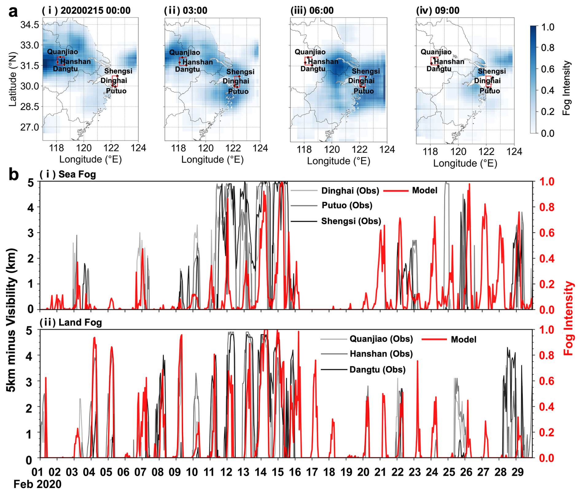
Figure 4 Validation of simulated sea-fog and land-fog intensity at representative coastal and inland stations. (a) Spatiotemporal evolution of a representative fog event on 15 February 2020. The red squares mark the validation stations used for the sea-fog and land-fog comparisons. (b) Temporal evolution of station-observed visibility reduction, expressed as 5000 m minus visibility, together with modelled fog intensity for representative sea-fog stations (i) and land-fog stations (ii). All times in the figure and its caption are given in local time (LT, UTC+8).

4.3 Variability of LVE area

In addition to LVE intensity, the spatial coverage of each LVE type was analysed. All hourly results for February and July 2020 were selected to represent the cold and warm seasons, respectively. Figure 5 reveals clear seasonal differences among the four LVE types. Land fog-haze showed the strongest contrast. Its area was negligible in July (Fig. 5b(ii) and c(ii)), and its accumulated winter area was approximately 21.0 times the summer value (Fig. 5a(ii) and a(iv)). The accumulated winter land-haze area was also approximately 1.7 times the summer value (Fig. 5a(ii) and a(iv)). These results are consistent with stronger aerosol accumulation during the cold season (Zhang et al., 2012). Sea fog also covered a larger area in winter. Its peak median area was approximately 1.75 times the summer value (Fig. 5b(iv) and c(iv)), and its accumulated winter area was approximately 1.8 times the summer value (Fig. 5a(ii) and a(iv)). Land fog showed a weaker seasonal contrast. Its maximum winter area was approximately 1.5 times the summer value, reaching about 140 000 km² in February and 95 000 km² in July (Fig. 5a(i) and a(iii)). The larger winter maximum is consistent with stronger radiative cooling and more extensive fog formation (Roach et al., 1976; Niu et al., 2010). Despite this difference, the accumulated land-fog area was similar in the two seasons (Fig. 5a(ii) and a(iv)). This similarity likely reflects more frequent summer fog formation under moist coastal conditions, which offsets the smaller summer event size.

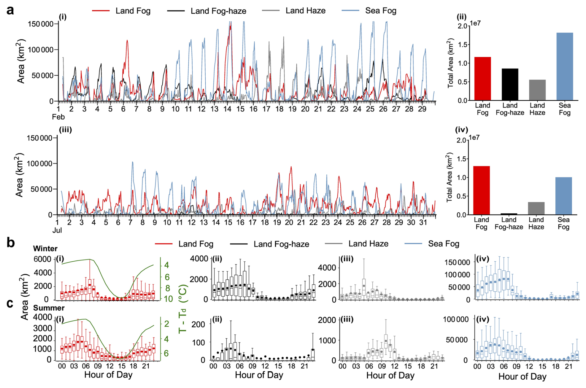
Figure 5 Temporal variations of low-visibility event areas in winter (February) and summer (July). (a) Time series (i, iii) and total accumulated areas (ii, iv) for land fog (red), land fog-haze (black), land haze (grey), and sea fog (blue). (b, c) Diurnal variations of event areas for (i) land fog, (ii) land fog-haze, (iii) land haze, and (iv) sea fog in (b) winter and (c) summer. Green lines in (i) represent the temperature–dewpoint spread (T−T_d). Box plots indicate the median (line), mean (dot), interquartile range (box), and data range (whiskers). All times in the figure and its caption are given in local time (LT, UTC+8).

The diurnal variations of the four LVE types exhibited distinct patterns (Fig. 5b and c). Generally, land-based fog and fog-haze aligned with the diurnal cycle of near-surface saturation, peaking before dawn and dissipating post-sunrise. This behavior corroborates the mechanism of classic radiation fog, driven by nocturnal radiative cooling and rapid dissipation via solar heating (Roach et al., 1976). For land fog, the peak coverage occurred later in winter (07:00–08:00) compared to summer (05:00–06:00) (Fig. 5b(i)), primarily attributed to the delayed sunrise and weaker solar radiation in the cold season, which retards the dissipation process. The land fog-haze showed similar start and dissipating time with land fog, but with substantially larger coverage in winter than summer due to the higher pollution in the cold season (Fig. 5b(ii) and c(ii)). Fog-haze began to accumulate slightly earlier than land fog. This earlier onset may reflect aerosol accumulation in the shallow nocturnal boundary layer. In winter, the area of dry haze peaked during the nocturnal and early morning hours (05:00) (Fig. 5b(iii)). Following sunrise, the development and deepening of the boundary layer enhance vertical mixing and dispersion, leading to a rapid decrease in winter haze area, which reaches its daily minimum in the afternoon (15:00). In summer, haze area was minimal overnight, increased after sunrise, and peaked from late morning to midday (10:00–13:00). Strong solar radiation promoted photochemical secondary aerosol formation during this period. This production partly offset dilution by daytime mixing. These patterns agree with previous observations of nighttime PM_2.5 accumulation in winter and daytime maxima in summer (Wu et al., 2024). Winter sea fog mainly dissipated after sunrise, whereas summer sea fog often persisted into midday and dissipated more slowly than summer land fog (Fig. 5b(iv) and c(iv)). The longer summer persistence is consistent with the weak diurnal variation in sea surface temperature, which limits daytime warming of the marine boundary layer and delays sea-fog dissipation (Koračin et al., 2014).

4.4 Sensitivity of fog-haze events to PM_2.5 mitigation

The model established above allows us to quantify the impacts of PM_2.5 on the formation of fog-haze. The sensitivity experiments are hereby performed by systematically adjusting PM_2.5 concentration inputs in the validated Sat-PM model. A case study from 9 February 2020 (Fig. 6a) showed that under original PM_2.5 levels, the model identifies a large, intense patch of fog-haze (red shading) over land. As PM_2.5 concentrations progressively reduce to 80 %, 60 %, and 40 %, the model shows the reduced intensity of fog-haze but increased clean fog, indicating the importance of PM_2.5 in transforming fog into fog-haze. The fog-haze area change corresponding to the PM_2.5 change for the whole month is shown in Fig. 6c. The quantitative sensitivity analysis uses all hourly results for February. The baseline simulation (with original PM_2.5) shows multiple large-scale fog-haze events, with peak area exceeding 70 000 km². Relative to the baseline, reducing PM_2.5 to 80 %, 60 % and 40 % of its original level decreased the mean February fog-haze area by approximately 43 %, 75 % and 95 %, respectively (Fig. 6e). The reduction to 80 % consistently lowered the event peaks, whereas the reduction to 60 % suppressed most large scale fog-haze events. This confirms that the spatial coverage of fog-haze is highly sensitive to PM_2.5 levels.

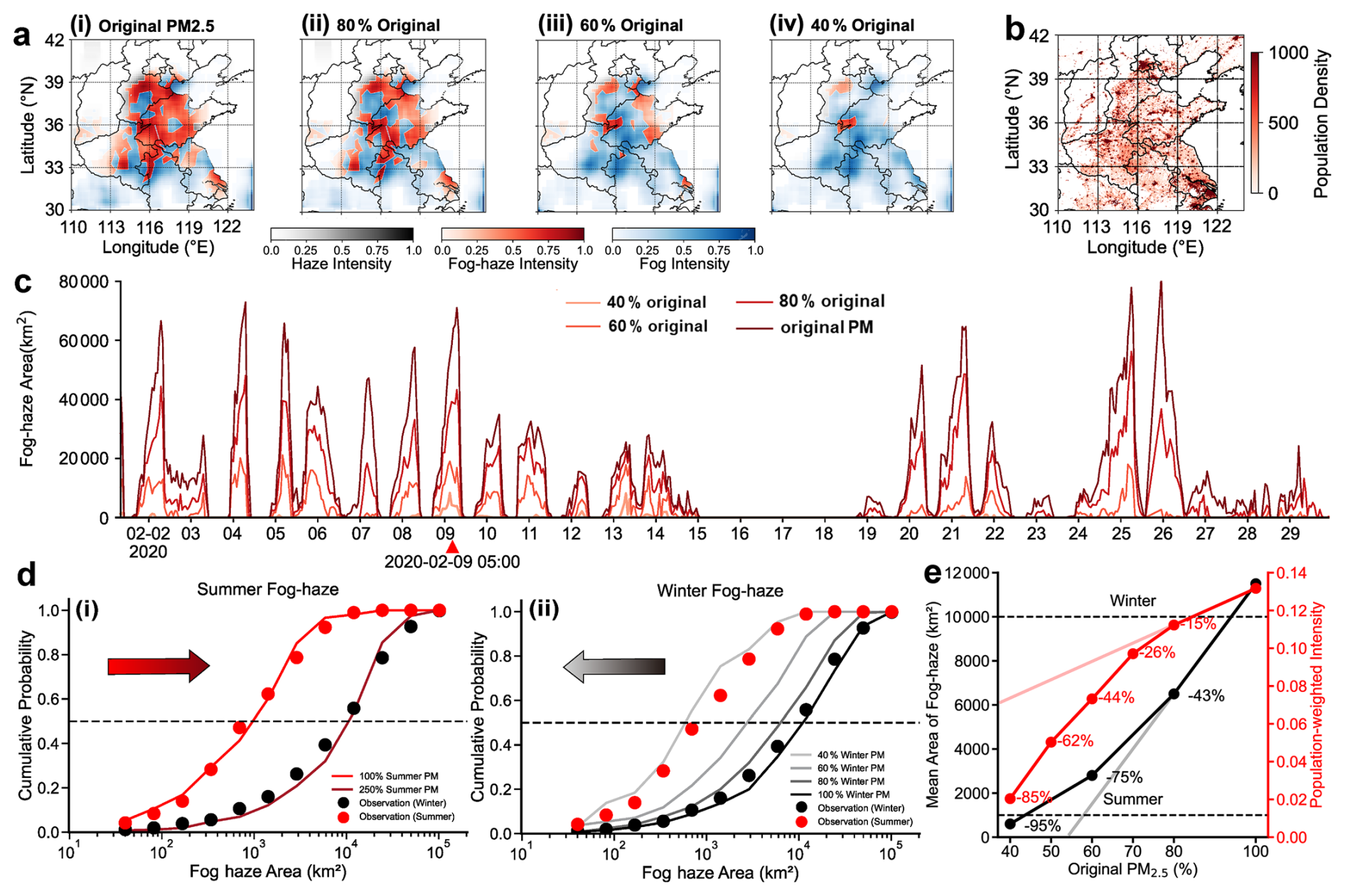
Figure 6 Sensitivity investigation on the fog-haze area to PM_2.5 concentration. (a) Simulated fog-haze spatial distributions with varying PM_2.5 levels at 05:00 LT on 9 February 2020: (i) original, (ii) 80 %, (iii) 60 %, and (iv) 40 % original concentrations. (b) Population density in the study domain. (c) Time series of the hourly fog-haze area in February 2020 by varying PM_2.5 concentrations in the study domain. (d) The cumulative probability of observed fog-haze area in February and July 2020 (the dots), with arrows showing the direction of simulated PM_2.5 variation, and (i) the simulation with original and 250 % of summer PM_2.5 concentrations (the red lines), and (ii) the simulation with original, 40 %, 60 % and 80 % of winter PM_2.5 concentrations (the grey lines). (e) Simulated response of the mean fog-haze area and population exposure to PM_2.5 reduction. All times in the figure and its caption are given in local time (LT, UTC+8).

The cumulative probability distribution function (CDF) of fog-haze area in the study region demonstrates the consistency between model simulation and observation (Fig. 6d). The mean fog-haze area (50 % CDF) is 9799 and 828 km² for February and July, respectively. Since the observed mean summer-to-winter PM_2.5 ratio is approximately 0.42 (Fig. S4 in the Supplement), reducing wintertime PM_2.5 concentrations to 40 % can simulate the summer-like aerosol conditions (Fig. 6d(ii)), and the resulting winter simulation curve (gray line) closely aligns with the observed summer distribution (red dots). Only the winter PM_2.5 input was scaled, while all satellite and meteorological inputs remained unchanged. The experiment therefore evaluates the PM_2.5 response under fixed winter meteorological conditions. The agreement with the observed summer distribution indicates the contribution of aerosol loading to the seasonal contrast in fog-haze area, rather than reproducing full summer conditions. Conversely, increasing summer PM_2.5 to 250 % can allow the summer simulation to align with the observed winter distribution (black dots) (Fig. 6d(i)). These results indicate that PM_2.5 loading contributes substantially to the larger diagnosed fog-haze area in winter under fixed meteorological conditions. Reduced PM_2.5 also increased clean-fog coverage and occurrence probability (Fig. S5 in the Supplement), indicating that some diagnosed low-visibility conditions shifted from fog-haze to clean fog.

Figure 6e further shows a nonlinear response of fog-haze area and population exposure to PM_2.5 reduction. Reducing PM_2.5 from 100 % to 80 % of its original level decreased the mean fog-haze area by 43 %, but reduced population exposure by only 15 %. Further reductions produced progressively larger decreases in fog-haze area, whereas population exposure responded more strongly only when PM_2.5 fell below 60 % of its original level. After a reduction of more than 40 %, an additional 10 % reduction in PM_2.5 decreased population exposure by 18 %, and exposure declined faster than fog-haze area.

5 Discussion

Independent test data and station observations support the application of the multi-source framework to regional LVE classification and intensity mapping. Station-level correlations between modelled LVE intensity and observed visibility reduction further show that the output represents event intensity rather than only binary low-visibility conditions (Figs. S6b, c and S7). The ablation experiments also show that satellite, meteorological and PM_2.5 data provide complementary information. Removing PM_2.5 reduced the performance of land low-visibility detection, whereas the attention-based CNN provided the most balanced performance among the tested architectures (Tables S3 and S4).

Seasonal controls differed among LVE types. Winter land fog reached a larger maximum area than summer land fog. Stronger radiative cooling in winter promoted near-surface saturation and favored extensive fog formation (Roach et al., 1976; Mason, 1982). However, cumulative land-fog coverage was similar in the two seasons. More frequent fog formation under moist summer coastal conditions compensated for the smaller event size. Thus, season affected the maximum extent of land fog more strongly than its cumulative coverage. Land fog-haze and dry haze showed stronger winter enhancement. Weak boundary-layer ventilation favours aerosol accumulation during winter. The larger winter fog-haze coverage therefore reflects both favourable saturation conditions and higher aerosol loading. Winter haze was largest at night and in the early morning. Boundary-layer growth after sunrise promoted vertical mixing and pollutant dilution. Unlike winter haze, summer haze increased after sunrise and peaked from late morning to midday. This daytime maximum is consistent with enhanced photochemical production under stronger solar radiation (Sun et al., 2016; Wu et al., 2024). Sea fog persisted longer in summer than in winter. Winter sea fog mainly dissipated after sunrise, whereas summer sea fog often continued into midday. The slower summer dissipation is consistent with the weak diurnal variation of the sea surface and the stability of the marine boundary layer, which reduces the immediate effect of daytime solar heating (Ma et al., 2014; Wagh et al., 2021). These results show that land fog, land fog-haze, dry haze and sea fog should not be treated as a single low-visibility phenomenon.

The PM_2.5 sensitivity experiments clarify the seasonal contrast in fog-haze. They quantify the response of fog-haze to prescribed changes in aerosol loading. Reducing winter PM_2.5 to 40 % of its original level shifted the simulated cumulative distribution of fog-haze area towards the observed summer distribution. Increasing summer PM_2.5 to 250 % produced a distribution closer to the observed winter distribution (Fig. 6d). These results suggest that aerosol loading contributes substantially to the larger winter fog-haze coverage. Under comparable saturation and liquid-water conditions, higher aerosol loading can increase CCN abundance and favour the formation of more numerous, smaller droplets. The larger total droplet surface area enhances light extinction (Twomey, 1977; Jia et al., 2026). Humid conditions promote aerosol hygroscopic growth and aqueous-phase processing, which can further increase particle mass and extinction (Peng et al., 2021; Zhong et al., 2018). Under real atmospheric conditions, aerosol–radiation interactions can reduce surface heating and suppress boundary-layer growth. This effect can promote the accumulation of aerosols and moisture near the surface (Wu et al., 2019). The associated meteorological feedback is not represented because the meteorological fields were fixed. Under persistent saturation, lower PM_2.5 weakens aerosol-related extinction and reduces CCN-rich conditions. Consistent with the increased clean-fog coverage in Fig. S5, the model therefore reclassifies some fog-haze pixels as clean fog rather than clear conditions.

Fog-haze area and population exposure responded differently to PM_2.5 reduction (Fig. 6e). During the initial reduction stage, fog-haze area declined more rapidly than population exposure. Exposure became more responsive when PM_2.5 fell to approximately 60 % or below its original level. This lag resulted from the population weighting of the exposure metric. Initial reductions mainly removed fog-haze from less populated regions with weaker anthropogenic emissions, while the remaining events persisted in densely populated emission hotspots. After PM_2.5 had been reduced by more than 40 %, an additional 10 % reduction produced an 18 % decrease in population exposure. The 40 % reduction therefore represents an effective range under the tested winter conditions, rather than a universal critical threshold.

The spatial concentration of fog-haze in densely populated emission regions is relevant to potential population exposure. Under humid conditions, aqueous-phase processing promotes the formation of water-soluble secondary aerosols (Wang et al., 2020). These aerosol components may be more bioavailable after inhalation and may contribute to systemic effects (Pope III and Dockery, 2006; Miller et al., 2017). The population-weighted fog-haze intensity should therefore be interpreted as an indicator of potential exposure, not as a direct epidemiological estimate of health risk.

6 Conclusion

This study developed and validated a framework that integrates satellite observations, reanalysis meteorological data and ground-based air-quality data to identify and quantify low visibility events over eastern China. By distinguishing clean fog, polluted fog-haze, dry haze and sea fog, the framework resolves the relative roles of near-surface saturation and aerosol loading in regional visibility loss. The prescribed PM_2.5 experiments show that pollution control can change both the extent and the category of low visibility events. When saturation near the surface persists, polluted fog-haze may shift towards cleaner fog rather than disappear. This response is consistent with aerosol effects on optical extinction and aqueous processing (Zhong et al., 2018; Peng et al., 2021).

A further insight is that regional visibility improvement does not necessarily lead to a comparable reduction in population exposure. Initial reductions in fog-haze coverage can occur mainly in less populated areas, while substantial exposure remains in densely populated emission hotspots. This spatial concentration is relevant to health assessment because humid aerosol processing may increase the soluble fraction and potential biological availability of particulate matter (Pope III and Dockery, 2006; Miller et al., 2017; Wang et al., 2020). Air quality assessments should therefore combine LVE attribution with population weighting instead of using visibility improvement alone as a proxy for reduced exposure or health benefit. Integrating this framework with models that couple atmospheric chemistry and meteorology, together with health data, could extend LVE analysis from retrospective diagnosis to prospective evaluation of clean air policies.