Long-term land-atmosphere carbon monoxide exchange from a tall tower in a rural Central European region

The atmospheric trace gas carbon monoxide (CO) significantly influences the atmosphere's oxidative capacity and indirectly affects climate. However, the net land-atmosphere exchange of CO remains highly uncertain due to the scarcity of long-term monitoring. This study presents and analyses a 10-year-long CO flux data series from a tall-tower eddy covariance (EC) system operated in a rural Central European region. The measured fluxes were evaluated separately for vegetation-covered, (quasi)natural areas and for populated areas. The estimated monthly mean emissions from the populated areas varied between 12 and 110 $\mathrm{nmol}{\mathrm{m}}^{-\mathrm{2}}{\mathrm{s}}^{-\mathrm{1}}$, with the lowest value observed in July and the highest in January, respectively. The measured wintertime emissions from the populated areas significantly exceed the activity-based estimations, presumably due to underestimated emissions factors for residential heating. The vegetation-dominated sector (agricultural fields and forests) acted as a weak net CO source from April to September with an average emission of 0.58 $\mathrm{nmol}{\mathrm{m}}^{-\mathrm{2}}{\mathrm{s}}^{-\mathrm{1}}$ (monthly range 0.31–0.91 $\mathrm{nmol}{\mathrm{m}}^{-\mathrm{2}}{\mathrm{s}}^{-\mathrm{1}}$), with the highest value occurring in July. The diurnal peaks of the median hourly emissions can be observed around noon, and they range from 1.59 to 2.66 $\mathrm{nmol}{\mathrm{m}}^{-\mathrm{2}}{\mathrm{s}}^{-\mathrm{1}}$. The nighttime (20:00–04:00 local standard time (LST)) hourly median values range from −1.01 to +1.17 $\mathrm{nmol}{\mathrm{m}}^{-\mathrm{2}}{\mathrm{s}}^{-\mathrm{1}}$. Their deviations from zero are not statistically significant at a p<0.05 probability level. Solar radiation was identified as the primary driver of CO exchange. This study also demonstrates the advantages and challenges of tall-tower EC flux measurements.

1 Introduction

For many decades, carbon monoxide (CO) was primarily considered a dangerous, toxic component of urban and indoor air pollution (Horner, 2000). With the introduction of three-way catalytic converters in gasoline-powered vehicles and advances in combustion technologies, CO pollution has become less of a problem in cities, at least in the more developed parts of the world (Hedelius et al., 2021). However, CO is also an important trace component of the global atmosphere, playing a significant role in atmospheric chemical processes, governing the oxidative capacity, and, through these, indirectly influencing the atmospheric greenhouse effect and climate change (Szopa et al., 2023).

Carbon monoxide is oxidized by the hydroxyl radical (OH). The product of this chemical reaction is carbon dioxide (CO₂), which is the second most important greenhouse gas in the atmosphere after water vapor (Schmidt et al., 2010). The oxidation of CO by OH is a concurrent chemical reaction with the oxidation of methane (CH₄) by OH, which is the dominant sink of CH₄ in the troposphere. One of the reaction products is carbon monoxide itself (Gaubert et al., 2017). The reaction of OH with CO consumes about 40 % of OH radicals (Lelieveld et al., 2016; Zhao et al., 2020). Hence, any change in the atmospheric CO concentration influences the lifetime of CH₄, the third most important greenhouse gas after water vapor and CO₂, and thus, CO could be considered an indirect greenhouse gas. The oxidation of CO by OH also results in hydroperoxyl radicals. Hydroperoxyl radical is one of the key components of ozone formation in the troposphere (Crutzen et al., 1999). In addition to being a greenhouse gas, ozone is also a phytotoxic substance of environmental concern. All this underscores the importance of research focusing on the sources, sinks, and processes of atmospheric CO.

Almost half of the carbon monoxide in the atmosphere is derived from the oxidation of CH₄ and volatile organic compounds. One quarter comes from direct anthropogenic sources, and a roughly similar amount from biomass burning, which has large interannual variability. The source inventory is completed by a minor (∼7 %) biogenic and a practically negligible (<1 %) oceanic release (Zheng et al., 2019). In the recent compilation of Zheng et al. (2019), oxidation by OH is the only globally notable sink of CO. Other authors (e.g., Khalil et al., 1999; Pihlatie et al., 2016; Liu et al., 2018; and references from therein) suppose that soils are globally a small but not negligible sink of CO due to microbial oxidation processes (Ragsdale, 2004; King and Weber, 2007). Duncan et al. (2007) list several inversion studies, a part of which attributes up to 10 % of the global CO sink to the soil, while the others did not indicate a net soil sink. Their own model supposes that biogenic emissions are roughly balanced with the amount consumed by soils, and that these emissions exert no significant net influence on the global CO budget. The scarce availability of in-situ CO flux data comes from relatively few, mostly short-term measurements performed in a limited spatial context (using e.g. chambers and short (<5 m) eddy covariance (EC) towers), which cannot represent the wide variety of ecosystems, soil types, and climate conditions, and regional scale fluxes. The rate at which microorganisms consume CO may depend on the soil's organic content, porosity, temperature, and water content, among other factors. Meanwhile, the production rate of CO via thermal or photodegradation of living or dead organic matter may depend on the species of plant (Bruhn et al., 2013). Bruhn et al. (2013) conducted a 2-month survey over a grassland in Denmark using UV-transparent Plexiglas chambers and found that the grassland was a net sink in darkness and a net source in natural sunshine. Constant et al. (2008) came to the same conclusion after one year of CO-flux measurement over a grassland in Canada using the vertical gradient method at a 3 m-tall tower. However, the 20-month-long survey of Cowan et al. (2018) over a grazed grassland in Scotland indicated net emission from the soil-vegetation system. The nighttime fluxes were around zero. The measurements did not reflect a net soil sink, but the EC system used did not allow the separation of the fluxes from the vegetation and from the soil. Laasonen et al. (2025) performed a 2-year-long measurement series over an Arctic peatland in Sweden and concluded that part of the peatland could act as either a net source or sink, depending on soil moisture levels. However, the area as a whole, as represented by the measurements, acted as a net CO source. Laasonen (2021) studied three different ecological systems in Finland (6–23 months) and one in Kenya (1 month), and found all to be net CO sources, as the soil uptake was offset by emissions mainly driven by incoming solar radiation. The 22-month-long measurement by Murphy et al. (2023) over a fertilized and grazed grassland in Ireland did not show net CO uptake by soil either. Pihlatie et al. (2016) reported on a single season (from snowmelt to snowfall) of CO-flux measurements over an area cultivated with a perennial reed canary grassland in Finland. They found a seasonally variable net flux direction (net source/net sink). The represented area was a net source from mid-April to mid-June, and a net sink from mid-June to November. Integration of the fluxes over the 7 months of the measurements indicated a weak net soil uptake. Pihlatie et al. (2016) also list several earlier CO-flux monitoring projects from different parts of the world, which indicate a mixture of positive and negative CO fluxes between the surface and the atmosphere. Sun et al. (2018) also recorded net soil uptake during a project covering a late growing season (July–November) in a Scots pine forest in Finland. Based on two short measurement campaigns, van Asperen et al. (2024) concluded that soil sources dominate over soil sinks in tropical rainforests in Brazil.

The general conclusion is that the net biogenic CO exchange between the land surface (soil + vegetation) and the atmosphere is highly uncertain due to the limited number of measurement projects and the rather short (from a few days to about 2 years) monitoring periods. Although the biogenic surface-atmosphere exchange is not the major contributor to the atmospheric CO budget, due to the wide-ranging effects of carbon monoxide in the global environment, it is nevertheless important to clarify this contribution.

Most of the historic measurements applied the so-called chamber method, which involved open or closed, opaque or transparent chambers of various sizes. This labor-intensive method cannot cope with the heterogeneity of the soil; moreover, its spatial representativeness is rather limited. The micrometeorological methods suitable for continuous monitoring of CO-fluxes only appeared about a decade ago (Blomquist et al., 2012; van Asperen et al., 2015; Pihlatie et al., 2016). To date, only a few, mostly short-term projects lasting from a few days to a maximum of two years, have been published (Blomquist et al., 2012; van Asperen et al., 2015; Pihlatie et al., 2016; Cowan et al., 2018; Murphy et al., 2023; Laasonen et al., 2025). These studies used short, 2–4 m tall towers and focused on specific ecological systems. The use of taller towers comes with significant benefits, but also poses challenges (see e.g. Berger et al., 2001; Davis et al., 2003; Desai et al., 2015; Chi et al., 2019; Herig Coimbra et al., 2024; Hilland et al., 2025; and several other publications). Tall-tower measurements can provide landscape-scale surface-atmosphere exchange values over heterogeneous regions of up to 100 km² or more, according to the height of the tower (Kljun et al., 2002; Kljun et al., 2004; Barcza et al., 2009; Desai et al., 2015; Chi et al., 2019; Barcza et al., 2020). Depending on topography and land cover patchiness, flux measurements on tall towers can be more robustly upscaled than the data from specific ecosystems. At the same time, these flux measurements may become decoupled from the surface during low-level temperature inversions, and temporary accumulation of trace gases in the atmospheric layer below the measurement level (“storage”) may also cause methodological challenges (Haszpra et al., 2005).

This study focuses on a tall tower site in western Hungary. Here, atmospheric CO concentration monitoring started already in 2015. The high-frequency data acquisition and the availability of a co-located EC system for CO₂ ecosystem exchange measurements (Barcza et al., 2020) motivated the exploration of these measurements to determine the flux of CO between the surface and the atmosphere. We are aware of only a few recent short-term (<1 year) attempts to measure CO fluxes on tall towers (Herig Coimbra et al., 2025; Hilland et al., 2025). These measurements were performed in urban or semi-urban environments. Our study presents the first long-term, tall-tower-based, regionally representative CO flux data series for a rural environment (agricultural fields, small villages) for the 2015–2025 period.

The main goals of the present study are (1) to synthesize and interpret the 10-year-long CO flux observations at the Hegyhátsál tall tower site; (2) to distinguish areas that are more influenced by anthropogenic activity from those that are mainly associated with vegetation by applying a footprint model; (3) to quantify fluxes from these two land cover types; and (4) to identify environmental variables that might explain the observed CO emissions from the vegetation-dominated, (quasi)natural areas. We focused primarily on analyzing anthropogenic surface-atmosphere CO fluxes during winter and natural CO fluxes during summer. The study provides a unique dataset for the observation-based, regional-scale estimation of the CO budget, where the results can be used to refine emission inventories in Central Europe.

2 Measurements and methods

2.1 Site location

The Hegyhátsál tall-tower greenhouse gas monitoring station is located in a rural environment in western Hungary (46.956° N, 16.652° E, 248 m a.s.l.). It was established in 1993 and provides data for the Global Atmosphere Watch of the World Meteorological Organization (WIGOS ID: 0-348-4-16307), and weekly air samples are taken here for NOAA's Global Cooperative Flask Air Sampling Network (NOAA station ID: HUN). Since 2024, the site has also been operating as an ICOS Class 2 atmospheric site. The station is a 117 m-tall TV/radio transmitter tower (operated by Antenna Hungária Corp.) equipped with meteorological sensors and air intake tubes. The mean annual temperature in the region was 10.4 °C in 1991–2020 and increasing rapidly with time (0.54 ± 0.13 °C per decade). The average annual precipitation is 690 mm, showing no significant trend but a wide range of variation between 475 and 939 mm yr⁻¹ during the indicated period.

The station is located in a fairly flat region, in the vicinity of a small village called Hegyhátsál. During the 10 years of this study (July 2015–June 2025), the population of the settlement, with no industrial or commercial activities, gradually decreased from 160 to 141 people (Hungarian Central Statistical Office, 2025). The village, a potential anthropogenic CO source, is located in the northwest sector of the station, at a distance of 400–1200 m, while the prevailing wind directions (NNE and SSW) are perpendicular to this direction. Apart from the village, the tower is surrounded by a regionally typical mixture of agricultural fields (dominantly corn, winter wheat, and rape in crop rotation with small plots of other cultivars) and forest patches. For the identification of the land cover types, the National Ecosystem Base Map of Hungary (NÖSZTÉP) (Tanács et al., 2021) was used. This dataset classifies 56 land cover type categories and provides land cover information with a spatial resolution of 20 m×20 m (Fig. 1). The soil type in the region is “Lessivated brown forest soil” (Alfisol, according to the USDA system). The upper layer is generally 10–20 cm thick and has an organic matter content of 5 %–8 %.

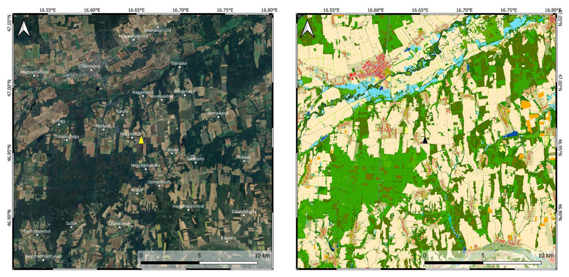
Figure 1 Google Earth satellite image (left – © Maxar Technologies/Google, 2025) and the NÖSZTÉP land cover map (right) of the region of the monitoring site (colors: shades of green – different types of forests and grasslands, yellow to pale orange – agricultural lands, bluish – wetlands, rivers, lakes, red/pink – buildings/residential areas, olive – green areas in residential environment; for detailed description see Tanács et al., 2021). The location of the tower is indicated by a yellow (left) and black (right) triangle.

The neighboring villages near Hegyhátsál are about 3 km away from the tower to the northwest (Katafa), west (Nádasd), and south (Hegyháthodász). The nearest settlement worth mentioning in the eastern sector is Gersekarát, located more than 7 km from the tower (Fig. 1). There is hardly any commercial or industrial activity in this predominantly agricultural region. The local roads connecting the small settlements carry little traffic (300–600 vehicle units per day). The only major road in the region is the 2×1-lane trans-European E65 running northwest–southeast with 5200 vehicle units per day (Magyar Közút, 2025). Its closest point to the monitoring site is about 500 m to the southwest.

2.2 Instrumentation

CO concentration has been monitored using an Enhanced Performance fast-response ${\mathrm{N}}_{\mathrm{2}}\mathrm{O}/\mathrm{CO}/{\mathrm{H}}_{\mathrm{2}}\mathrm{O}$ analyzer (Model 913-0014, Los Gatos Research Ltd., San Jose, CA, U.S.A.) with fast-flow optional accessories, which records at 5 Hz frequency continuously since July 2015. The analyzer is located at ground level in an air-conditioned room of the transmitter building. Air to be analyzed is taken from 82 m on the tower through an approximately 100 m-long $\mathrm{3}/\mathrm{8}$ in. OD Synflex 1300 tube (Eaton Corporation Plc, Dublin, Ireland). The flow rate of about 3.5 L min⁻¹ is maintained by a diaphragm vacuum pump (KNF Type N 880.3 AN.22E, Neuberger, Inc., Trenton, NJ, U.S.A.). The analyzer is regularly calibrated against four CO-in-natural air standards (48–513 nmol mol⁻¹) produced and certified by Max Planck Institute for Biogeochemistry, Jena, Germany, to meet the high accuracy requirements of the monitoring of the temporal variation in the concentration (long-term trend, seasonal and daily variations, etc.) (WMO, 2024). The standards are traceable to the WMO CO X2014A scale. The drifts of the standards were linearly corrected between the recalibrations of the standards, and we continuously compared the measurement results with those obtained from NOAA flask air samples to detect any significant drift. The EC system also includes a GILL R3-50 research ultrasonic anemometer. The ultrasonic anemometer and the air inlet are mounted at the end of a 4.4 m long north-looking instrument arm at 82 m above the ground, where the diameter of the steel-tube tower is 1.8 m. The distance of the air inlet from the center of the ultrasonic anemometer is 80 cm. Considering the high elevation of the EC system above the ground, where the characteristic size of the eddies is larger than that at the elevation of the usual EC systems (typically a few meters above the ground), the 5 Hz sampling frequency and the 3.5 L min⁻¹ flow rate proved sufficient for reliable flux calculations (Haszpra et al., 2018).

2.3 Auxiliary data

Since the monitoring system was originally designed for CO concentration rather than for a CO exchange study, only a few CO-flux-relevant auxiliary measurements are available from the site.

Instead of the standard height of 2 m, air temperature is available at 10 m elevation above the ground (until November 2022: Vaisala Model HMP35D; from December 2022: Vaisala Model HMP155; Vaisala Oyj, Helsinki, Finland), following the requirements of another research project (Haszpra et al., 2001). A Model LI-190SZ (LI-COR Inc., Lincoln, Nebraska, USA) quantum sensor was available until March 2021, followed by an Apogee SQ-100X-SS sensor (Apogee Instruments, Inc., Logan, Utah, USA) from December 2022 for recording the incoming photosynthetically active radiation (0.4–0.7 µm) at 2 m above the ground.

UV radiation and soil water content (SWC) measurements are not available at the tower. These variables are mentioned in the literature as potential drivers of the CO exchange between the surface (vegetation + soil) and the atmosphere (Bruhn et al., 2013; Murphy et al., 2023; Laasonen et al., 2025); therefore, we turned to the ERA5 reanalysis dataset of the European Centre for Medium-Range Weather Forecasts (Copernicus Climate Change Service, 2022). Downward UV radiation at the surface (0.20–0.44 µm) and volumetric soil water content in layer 0–7 cm data were downloaded for the nearest two grid points to the monitoring station (47.0° N, 16.5° E; 47.0° N, 16.75° E), and were then averaged.

A disadvantage of tall-tower EC systems is that they may be decoupled from the surface by low-level inversions from time to time (Desai et al., 2015; Chi et al., 2019). In these situations, the EC systems cannot provide the actual surface–atmosphere flux data. To remove decoupled measurements in cases of low-level inversion, information on the height of the boundary layer was also derived from the ERA5 reanalysis dataset.

2.4 Flux calculation

The basic theory of the EC flux measurement technique is discussed in the scientific literature in detail (see e.g. Aubinet et al., 2012, for summary and review). The methodology applied for the calculation of the hourly turbulent fluxes of CO at our tall tower monitoring site was originally developed for CO₂ flux derivation (Barcza, 2001; Haszpra et al., 2005; Barcza et al., 2020), and has been adapted to calculate the exchange of CO. In the following, we provide a brief summary of the methodology. For more details, the reader is referred to Barcza (2001), Haszpra et al. (2018), and Barcza et al. (2020).

As a first step, the lag time caused by the ∼100 m long air intake tube is determined. The H₂O lag time is used as an indicator for the identification of the CO lag time. It is typically 5–10 s longer than the lag time for CO due to the adsorption/desorption of water vapor on the inlet tube wall. For each day, the lag time is manually determined by visualizing the lagged covariance data for all 24 h. This method was chosen because the covariance maximization would frequently lead to erroneous lag time values for days with low turbulent flux (cf. Supplementary material S2 in Haszpra et al., 2018). Assuming a constant lag time for each particular day is supported by the relatively constant performance of the pump and the visual inspection of the dataset over the 10-year-long measurement period. For low flux days, the lag time can be determined from the lag time from previous days with larger fluxes, and with careful visual selection of some of the lagged covariance curves that correctly indicate the true value (e.g. associated with occasional higher fluxes).

Angle-of-attack dependent calibration is applied to the raw sonic anemometer data (van der Molen et al., 2004). Since the EC system is located at a height of 82 m, the slight tilt of the sonic anemometer, the tower body structure, and the surrounding terrain can affect the mean airflow that is sampled by the anemometer. We hence chose the three-dimensional wind vector rotation to align the coordinate system with the prevailing streamlines (Lee, 1998). This method performed better for our site than the popular planar fit method and the simple 2D rotation (Aubinet et al., 2012). Using the technique detailed in Barcza (2001), rotation coefficients are calculated for each 3° wind direction sector using data from long time periods. The length of the time periods is determined by the timing of interventions when the tilt of the anemometer might have changed due to maintenance work. These coefficients are used to determine the rotation angle of the 3D wind for a given wind direction (see Fig. 2.12 in Barcza, 2001), which means that the rotated coordinate system matches the mean streamlines (but allows non-zero mean vertical wind speed – Lee, 1998). Linear detrending is applied to the wind and CO mole fraction time series.

The hourly means of the turbulent fluxes are calculated taking into account the predetermined lag times and rotated 3D wind data described above. As the system derives fluxes from dry air mole fractions of CO, the Webb-Pearman-Leuning correction (Webb et al., 1980) was not applied. As part of the postprocessing, spectral corrections are applied to account for flux losses caused by the fluctuation damping caused by the intake tube, lateral sensor separation, sensor line averaging, etc. (Moore, 1986; Massman, 1991). Finally, several quality control indicators are derived (Vickers and Mahrt, 1997; Kroon et al., 2010).

An EC system measures the mass transport through a horizontal plane at its elevation above the ground, which is 82 m in our case. In situations of limited vertical mixing, the EC system may become decoupled from the surface, leading to measurements that are no longer representative of the actual surface processes. To avoid such values, we rejected fluxes when the boundary layer height was below 100 m. The layer below the EC system may become enriched (surface source) or depleted (surface sink) in the trace gas studied without recording. After the decoupling (i.e., during the breakup of the nighttime inversion after sunrise), the accumulated excess or deficiency in the surface layer appears in the measured flux (storage flux). Although the temporary decoupling may distort the measured diurnal variation, the daily total flux properly reflects the daily surface-atmosphere exchange (as there is no long-term accumulation or depletion below the measurement level; cf. Haszpra et al., 2005). Unlike in the case of CO₂, we hypothesize that emitted CO is neither taken up nor reemitted during the time of decoupling, i.e., there should not be any distortion of the net CO exchange estimations.

To test this hypothesis, we calculated the single-point concentration-based CO storage flux (assuming a constant vertical CO mole fraction profile up to the measurement level – Greco and Baldocchi, 1996). The result showed that the CO storage term at 82 m is relevant for the CO fluxes only in the winter season, redistributing the hourly fluxes slightly, but not affecting the total flux. It is important to mention that the variability of the fluxes is high (see Results), and as the single-point-based storage flux calculation is only a simple approximation of the true storage flux (where the latter is supposed to take into account the non-linear shape change of the CO profile as well), consideration of the storage flux increases the uncertainty. As the analysis is restricted to turbulent conditions ($u_{\ast }\ge \mathrm{0.2}$ m s⁻¹, PBLH≥100 m – see Sect. 2.5), to ensure that the surface fluxes are identical with the measured CO flux measured at 82 m elevation, the storage-prone hours are largely excluded beforehand. Thus, it seems reasonable to accept the aforementioned hypothesis on the negligible effect of CO storage flux on the results.

Considering quality control and data flagging based on the calculated quality indicators (Vickers and Mahrt, 1997; Kroon et al., 2010), an attempt was made to check their applicability to filter outliers. However, as there was no detectable relationship between the magnitude of the CO fluxes and the indicators, this filtering was not applied. Another approach would have been to filter the data based on statistical measures (e.g. removing data outside the ±3 standard deviation threshold or using percentile-based filtering, etc.). We rejected this approach because we expect significantly different fluxes from the different land cover types (arable lands, forests, villages, etc.) in the heterogeneous landscape surrounding the tower. Hence, no outlier filtering was applied during the flux calculation. It is important to note that the prerequisites for the footprint calculations inherently filter out low wind speed conditions (i.e. strong inversion during nighttime), which represents an alternative quality control.

2.5 Flux footprint calculation

The flux footprint function quantifies the relative contribution of each element of the upwind surface area to the measured flux as a probability density function. For the calculation of the source area (footprint) of the flux measurements, the two-dimensional Flux Footprint Prediction (FFP) model developed by Kljun et al. (2015) was applied. This model performed amongst the best in a test against data from a tracer release experiment involving several footprint models (Heidbach et al., 2017) and is, unlike other models, valid for tall tower fluxes.

The input parameters of the model are the measurement height above displacement height (z_m), the roughness length (z₀), the Monin-Obukhov length (L), the standard deviation of the lateral wind speed (σ_v), the friction velocity (u_∗), and the height of the boundary layer (h). The wind direction is an optional input parameter, but it is needed here for the spatial attribution of the source areas. As wind direction is affected by the tower body (see Barcza, 2001), we developed a wind direction correction method based on the co-located short-tower (3 m) EC system documented in Barcza et al. (2003). The wind direction measured at the height of 82 m is empirically adjusted based on the wind direction climatology of the short tower (3 m), taking into account the changes in wind direction with height. This method was successfully used in earlier studies (Barcza et al., 2009; Gelybó et al., 2013) focusing on footprint analysis based on the tower data.

As it was mentioned above, the tower body structure affects the airflow sampled by the eddy covariance system in the case of southerly winds (see Fig. 2.12 in Barcza, 2001). Although the wind direction correction aligns the footprint well facing the mean wind direction for a given hour, the distorted turbulence might affect the source region detection and also the measured CO flux itself due to possible modification of the spectral properties of the vertical wind speed. We have quantified the potential effects of the flow distortion within the wind sector in question (between 155 and 215°). It was found that although σ_v is systematically affected by the tower body within the sector, the footprint geometry remains largely unaffected (the width of the footprint changes slightly but does not affect the results). We also tested the option to drop all CO fluxes measured from wind directions between 155 and 215°. Statistical analysis indicated that CO flux filtering inevitably increases uncertainty but leads to the same conclusions, so keeping all data supports a more statistically sound estimation. It is important to note that southerly winds bring information from the (quasi)natural areas where the fluxes are considerably smaller than those originating from the populated areas (see Results).

Displacement height was considered to be negligible relative to the height of the measurements; thus, the observation height was used to approximate z_m. The listed parameters were either directly measured or could be calculated from the measurements. The boundary layer height was available from the ERA5 reanalysis dataset (see Sect. 2.3) for the region of the tower. The roughness length was assumed to be equal to 0.15 m based on estimates from an earlier study (Barcza et al., 2009).

In this study, following the recommendations for the application of the FFP model (Kljun et al., 2015), the model was used with the following restrictions: $\mathrm{20}{z}_{\mathrm{0}}<z_{\mathrm{m}}<h_{\mathrm{e}}$, $-\mathrm{15.5}\le z_{\mathrm{m}}/L$, where h_e is the height of the entrainment layer. h_e is typically around 0.8 h (Holtslag and Nieuwstadt, 1986). We also applied $u_{\ast }\ge \mathrm{0.2}$ m s⁻¹ to ensure turbulent forcing.

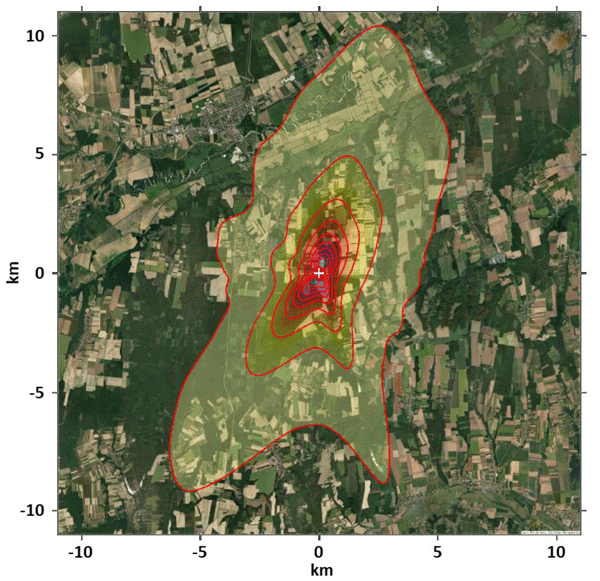
An example footprint climatology of the station for the year 2020 is presented in Fig. 2. It demonstrates that the prevailing wind directions at the station are northeasterly and southwesterly, and that the footprints for these wind directions typically extend up to 10 km from the tower.

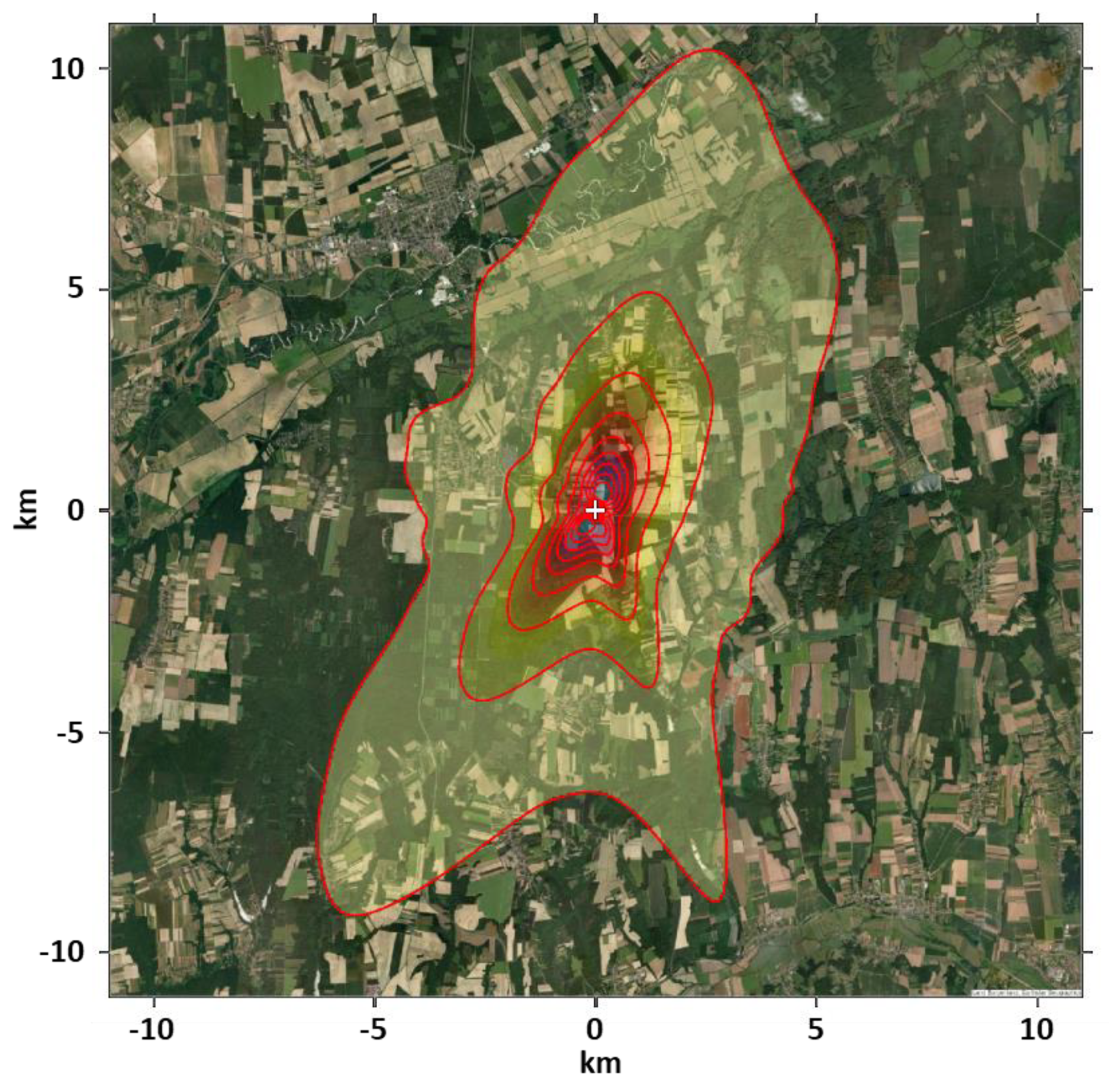
Figure 2 Flux footprint climatology of the monitoring site in 2020. For data selection, see Sect. 2.6. The footprint contour lines (red) show a 10 %–90 % contribution to the flux measurement in 10 % steps. The tower is at the origin (0,0) of the map, and it is indicated by a white “+” sign. Source of base map: Esri | Powered by Esri.

2.6 Data availability statistics

The measurements started on 1 July 2015, and the present study evaluates the data until 30 June 2025. The 10-year-long data series comprises 87 672 hourly values. During a total of 21 802 h, predominantly on summer nights and at any time of day in winter (see the boundary layer height statistics in Haszpra and Barcza, 2010), the boundary layer height was below 100 m. Due to the potential decoupling of the EC system from the surface, we rejected these data points for surface flux estimation. In the case of an additional 16 499 h, fluxes could not be calculated for technical reasons (power outage, lag time, instrument malfunction, data acquisition gaps, maintenance, etc.). Finally, 14 068 h did not satisfy the conditions for footprint calculations. In the absence of a solid theoretical basis, and also to avoid inclusion of modelled data, data gap filling was not applied.

Far-reaching flux footprints are increasingly uncertain and may cover distant anthropogenic sources, distorting the regional emission estimations. To decrease attribution uncertainty, we selected only those footprints for which the integral of the footprint transfer function over a radius of 5 km from the tower was ≥0.8, i.e., the footprint contribution to the fluxes measured at the tower was ≥80 %. Altogether, we had to exclude 70.4 % of the hourly data; that is, 25 917 hourly data remained available for the actual study.

2.7 Flux map, and separation of populated and (quasi)natural areas

In the case of most conventional EC towers, which are only a few meters tall, the heterogeneity of the footprint area is generally small. However, in the case of tall towers with an extensive footprint area, it can be significant. While tall towers are great for determining the average emissions of heterogeneous areas (Desai et al., 2015; Peltola et al., 2015; Chi et al., 2019) and allow more reliable upscaling of the results, attempts can also be made to separate fluxes from areas with different land cover types (Barcza et al., 2009; Helbig et al., 2017; Tuovinen et al., 2019; Hernandez Rodriguez et al., 2023; Tikkasalo et al., 2025; Molinier et al., 2026).

In this study, we use a simple method to determine the CO flux of populated grid cells and (quasi)natural grid cells separately. A grid cell is considered “populated” if it belongs to one of the following NÖSZTÉP land use categories: buildings, roads, other paved or unpaved artificial surfaces, as well as green fields in an artificial environment. The term “(quasi)natural grid cell” or “vegetation-covered grid cell” (these terms are used as synonyms in this paper) refers to the categories of arable land, forest, grassland, and wetland, where the anthropogenic emissions are assumed to be minimal. Due to the relatively small amount of data, we did not attempt to separate the fluxes from agricultural fields and forests.

Using the filtered CO fluxes, footprint-weighted flux maps were calculated. In these maps, each grid cell contains the average of the fluxes measured at the tower weighted by the value of the footprint transfer function at the given grid cell. To provide a robust estimation at low data availability, the quantification of CO flux from the populated areas and from the (quasi)natural areas was performed in monthly time steps. The hourly CO fluxes were combined with the footprint analysis and the land cover map to quantify the percentage of contribution from both the populated and (quasi)natural areas.

At any time, the measured flux (f) is assumed to be the sum of the flux from the populated areas (F) and that from the non-populated, (quasi)natural areas (f_bg). For the determination of the emissions from the populated areas, the following model was used:

$$\begin{array}{}\text{(1)}& F=(f-f_{\text{bg}}(\mathrm{1}-\mathit{\alpha }\left)\right)/\mathit{\alpha },\end{array}$$

where α is the contribution of the populated grid cells. Assuming at least an order of magnitude difference between the fluxes from the populated areas and from the (quasi)natural areas (“background flux”), we used the initial guess of f_bg = 0 for the calculation. We used the emission density estimated this way for the populated grid cells (F) to make a more realistic estimation of f_bg using an iterative procedure.

Using the estimated emission value from the populated grid cells (F), and rearranging Eq. (1), we can express the CO exchange of the (quasi)natural grid cells (f_bg):

$$\begin{array}{}\text{(2)}& f_{\text{bg}}=(f-\mathit{\alpha }F)/(\mathrm{1}-\mathit{\alpha }).\end{array}$$

Substituting the calculated f_bg value back into Eq. (1) yields a modified F value, which is then used again in Eq. (2). We repeated the process until F and f_bg no longer changed significantly from one iteration to the next.

If there are only a few populated grid cells within the footprint, they are not necessarily representative of the populated areas in general. Therefore, the higher the α-value, the more robust the estimation. On the other hand, a higher α-value implies that less data are available for the calculations, which reduces the accuracy of the estimations. To find a compromise, we examined how the value of F depends on the α-value. What is the α-value such that, if increased further, the value of F no longer changes significantly? This threshold value and the related F values were used in the further calculations.

3 Results

3.1 Directional distribution of carbon monoxide flux

Figure 3 shows the footprint-weighted flux maps for the summer and winter months separately for the entire measurement period. The figure shows that the flux is higher from the direction of the village (west-northwest) than from the sector dominated by agricultural fields and forests. This result provides a solid basis for the separation of the populated (i.e. anthropogenic emission related) and dominantly natural areas with vegetation cover.

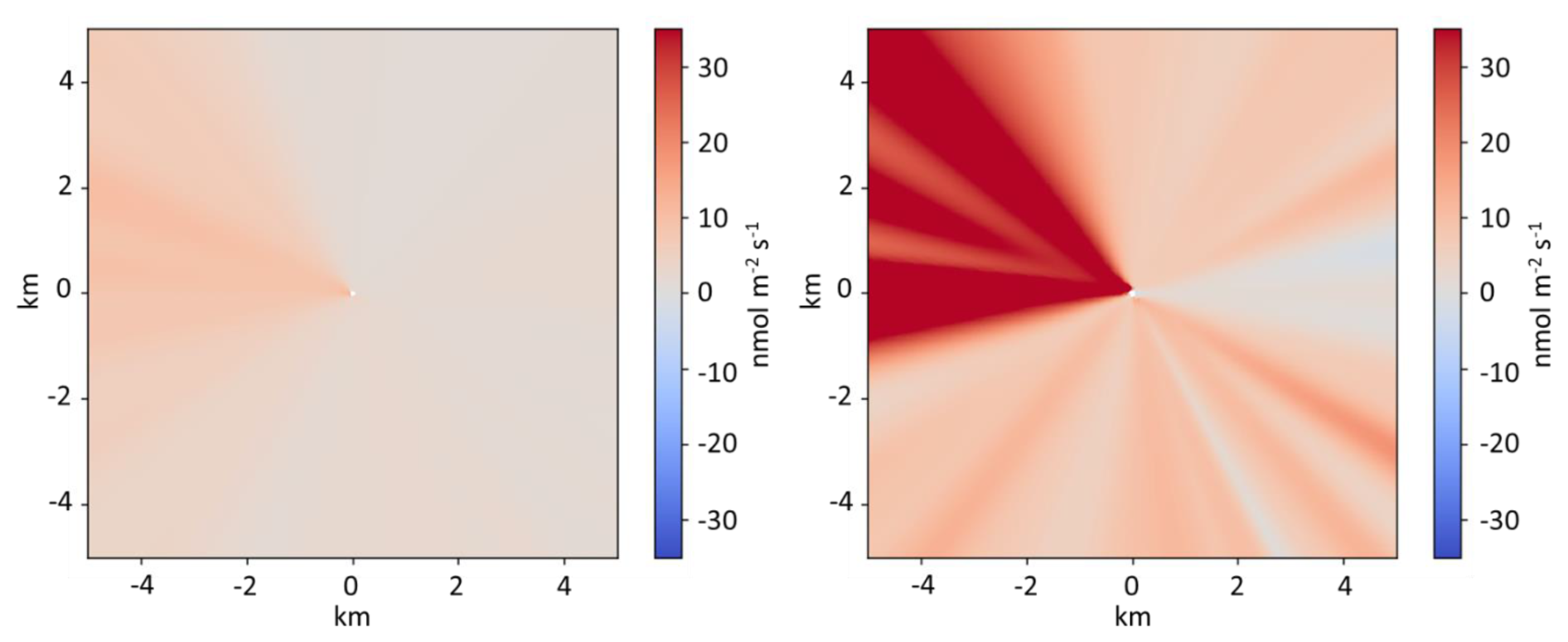
Figure 3 Footprint-weighted flux maps for the summer (June–August, 2015–2025, left) and winter months (December–February, 2015–2025, right). The maps are based on cases in which the footprint contribution over a radius of 5 km from the tower is at least 80 % of the measured fluxes. The tower is at the origin (0,0).

3.2 Carbon monoxide emission from the populated areas

Based on the data selection described in Sect. 2.6 and source area separation presented in Sect. 2.7, the flux contribution from the populated area of the nearby small village of Hegyhátsál can be up to 42 %. High values are typical when the wind blows from the west-northwest sector. In the same sector but farther from the tower (2.5–3.5 km), there is a larger village called Nádasd (population: 1300). In the case of far-reaching footprints in this direction, the flux contribution from this settlement may reach 14 %. Hegyháthodász, similar in population to Hegyhátsál, is located 1.8–2 km south of the tower. The flux contribution from this village may also reach 17 % during southerly winds. Neither of these settlements has notable industrial or commercial activities. Western Hungary, where the monitoring site is located, is not a fire-prone area; forest fires are rare, and open burning is prohibited in agricultural areas. Since CO measurements began in 2015, the closest fire event revealed by satellites (MODIS MCD64A1 Burned Area and MOD14 Active Fire products) was more than 20 km from the monitoring station, and even that was small in scale. Hence, CO emissions should primarily originate from domestic activities, such as residential heating, which is typical in winter, and from traffic year-round. Due to the absence of hot spots, it is assumed that anthropogenic emissions are uniformly distributed in the populated areas. Thus, the integrals of the footprint transfer function over these areas directly give their contributions to the measured flux.

Using the simple model presented in Sect. 2.7 (Eq. 1) to calculate monthly aggregated fluxes, a sensitivity analysis was performed to check the effect of flux contribution threshold selection on the aggregated CO flux. The calculated median emissions for the populated areas are presented in Fig. 4 for the cases when the flux contribution from the populated grid cells is ≥20 %, ≥25 %, ≥30 %, and ≥35 %, respectively. As can be seen in the figure, the differences are minimal. The significant seasonal variation and the small amount of available data for each month prevent the estimation of the diurnal variation of the fluxes. For the same reason, we could not estimate the 2015–2025 trend either. In the following, the calculations are based on the 2015–2025 median value calculated for those cases when the flux contribution from the populated grid cells is ≥25 %.

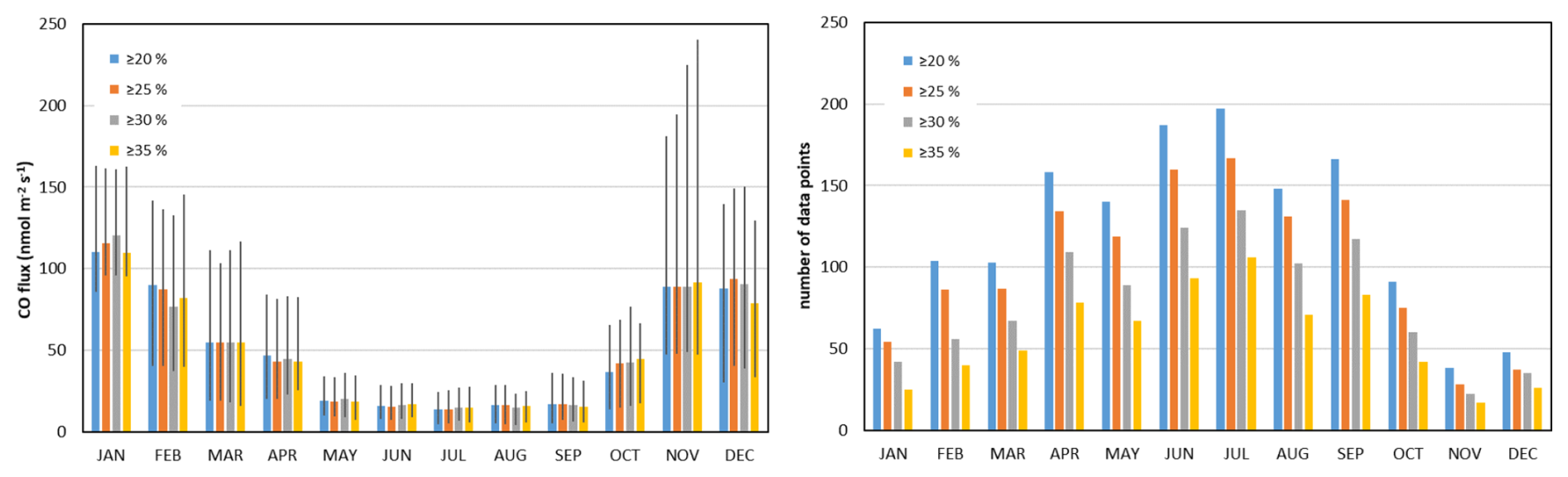
Figure 4 2015–2025 monthly mean carbon monoxide fluxes from the populated areas (left panel) and the number of data available for the calculations (right panel). The flux values are calculated for ≥20 %, ≥25 %, ≥30 %, and ≥35 % flux contribution from the populated grid cells (α-value), assuming zero net flux from the (quasi)natural grid cells. The whiskers indicate the lower and upper quartiles. The right panel shows the decreasing data availability with the increasing flux contribution (α-value).

3.3 Carbon monoxide exchange of the vegetation-dominated landscape, and the refinement of the emissions from populated areas

For flux measurements at a height of 82 m in a densely populated Central European region, it is practically impossible to exclude roads and small agricultural buildings from the footprints of the measurements in any direction. For the determination of the CO exchange of the vegetation-dominated, (quasi)natural landscape (agricultural fields, forests), we selected those hourly data points for which ≥80 % of flux footprint contribution came from within a 5 km radius of the tower (see also Sect. 2.6), and where the flux contribution from the so-called populated grid cells did not exceed 2.5 %. The median contribution of the populated grid cells to the measured fluxes over the 12 347 selected hours was 1.74 %. The contribution of arable land to the measured flux varied between 11 % and 78 %, while the corresponding values for forested areas were 7 % and 68 %, depending on the location and extent of the actual footprint. This sector characteristically corresponds to the wind directions of 350–150° and 190–230° (see Fig. 3).

Using the iterative method described in Sect. 2.7, Fig. 5 shows the changes in the calculated emissions from the populated grid cells in each month and in each iteration step. While the change in F was up to 13 % in the 1st iteration step, it was less than 0.4 % in the 2nd step, and less than 0.02 % in the 3rd step. It means that even after the 2nd round, the calculated fluxes for the populated areas hardly change. The results obtained in the 3rd iteration step are considered the actual emission densities of the populated grid cells, and are discussed further in Sect. 4.1. Using a ≥25 % threshold, the monthly CO fluxes range from 82–110 $\mathrm{nmol}{\mathrm{m}}^{-\mathrm{2}}{\mathrm{s}}^{-\mathrm{1}}$ in winter to 14–16 $\mathrm{nmol}{\mathrm{m}}^{-\mathrm{2}}{\mathrm{s}}^{-\mathrm{1}}$ in summer. Summer values are 85 % lower on average than the winter values, demonstrating the significant contribution from heating in the cold season.

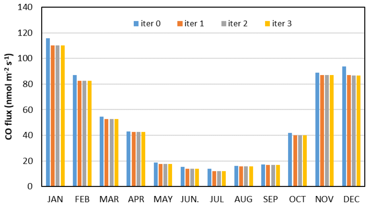
Figure 5 Iterative approximation of the emission density from the populated areas using the method described in the text. Iteration 0 (iter 0) represents the uncorrected data calculated in Sect. 3.2 (see Fig. 4). The flux values are calculated for the cases when the contribution of the populated grid cells to the measured fluxes at the tower is at least 25 %.

Figure 6 shows the mean diurnal variation of net CO exchange over the (quasi)natural grid cells for each month based on the converged data. Lacking an objective criterion for defining a data point as “extreme”, outlier removal was not applied during the quality control of the data (cf. Sect. 2.6). However, outliers (whether extreme or not) may distort the averages; therefore, Fig. 6 shows the median value for each hour of each month. The symbols in the figures indicate the confidence level of the deviations of the values from zero as determined by the Wilcoxon hypothesis test. It should be noted that significantly fewer data were available for nighttime hours than for daytime hours (especially in summer), affecting the confidence limits. As mentioned earlier, the limited data availability meant that the diurnal variation of the emission of the populated grid cells could not be derived. Therefore, the monthly average emissions were used to derive the natural CO flux, which can affect the estimated diurnal variation of the latter. Presumably, both anthropogenic and natural CO emissions are lower during night than during day; therefore, the limitation in the correction algorithm does not significantly alter the diurnal shape of the CO exchange over the arable land/forests.

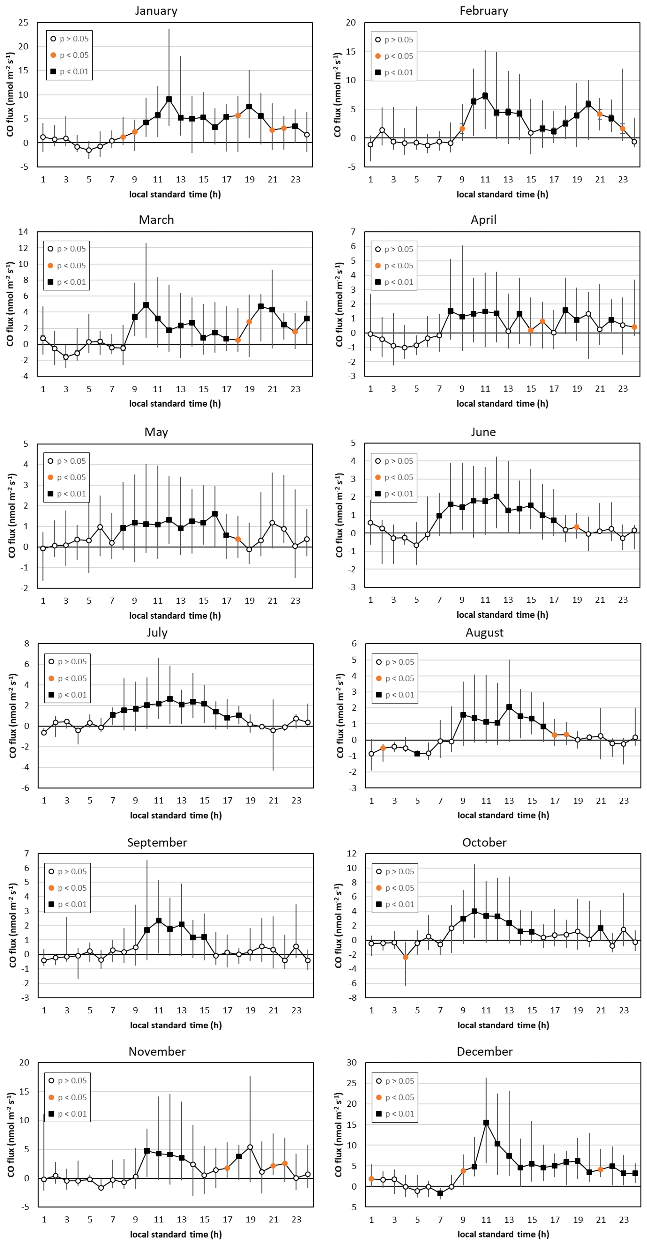
Figure 6 Mean diurnal variation of net CO exchange in the (quasi)natural grid cells (2015–2025) based on the converged data (α<2.5 %). Whiskers indicate the lower and upper quartiles, while the symbols give the probability level of the deviation of the median from zero. Note the different y axes.

The mean daily flux for each month can be calculated from the monthly mean diurnal variations of the hourly median fluxes (Fig. 7). Fluxes from the (quasi)natural grid cells are only a few percent (1 %–8 %) of those from the populated grid cells (Fig. 5). The winter maximum in the net exchange over the vegetated landscape cannot be explained by natural processes alone. It is hypothesized that our simple method cannot completely filter out the anthropogenic emissions. This question will be discussed further in Sect. 4.2.

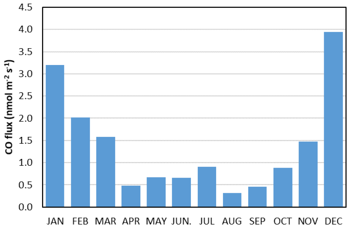
Figure 7 Seasonal variation of the monthly mean CO flux from the (quasi)natural grid cells (α<2.5 %).

The diurnal variation of the CO exchange in the arable land/forest (i.e. vegetation-covered) sector shows a daytime maximum, which is more pronounced during the summer half-year (Fig. 6). The nighttime net flux tends to be negative, though it does not deviate statistically significantly from zero throughout the year. The average emission for the summer half-year (April–September), when the unavoidable anthropogenic influence is the lowest, is 0.58 $\mathrm{nmol}{\mathrm{m}}^{-\mathrm{2}}{\mathrm{s}}^{-\mathrm{1}}$ based on the monthly averages calculated from the hourly median values. The range is 0.31–0.91 $\mathrm{nmol}{\mathrm{m}}^{-\mathrm{2}}{\mathrm{s}}^{-\mathrm{1}}$, with the highest value occurring in July. The daily peaks of the median hourly emissions range from 1.59 to 2.66 $\mathrm{nmol}{\mathrm{m}}^{-\mathrm{2}}{\mathrm{s}}^{-\mathrm{1}}$. The nighttime (20:00–04:00 LST) hourly median values range from −1.01 to +1.17 $\mathrm{nmol}{\mathrm{m}}^{-\mathrm{2}}{\mathrm{s}}^{-\mathrm{1}}$, respectively.

3.4 Possible drivers of the ecosystem carbon monoxide budget

We considered UV radiation, photosynthetically active radiation, daytime/nighttime air temperature, and soil water content as possible drivers. The correlation coefficients between these drivers and CO flux, as well as their probability levels, are presented in Fig. 8. The results suggest that solar radiation plays an important role in the CO emission of the soil/vegetation system. The correlation with air temperature at 10 m is not statistically significant at a reasonable probability level for most of the year (standard air temperature measurements or soil temperature data were not available at our site). The nighttime correlations between CO net flux and temperature are not significant either (Fig. 8), suggesting that the summer daytime correlation is the result of the high correlation between temperature and radiation (Fig. 9).

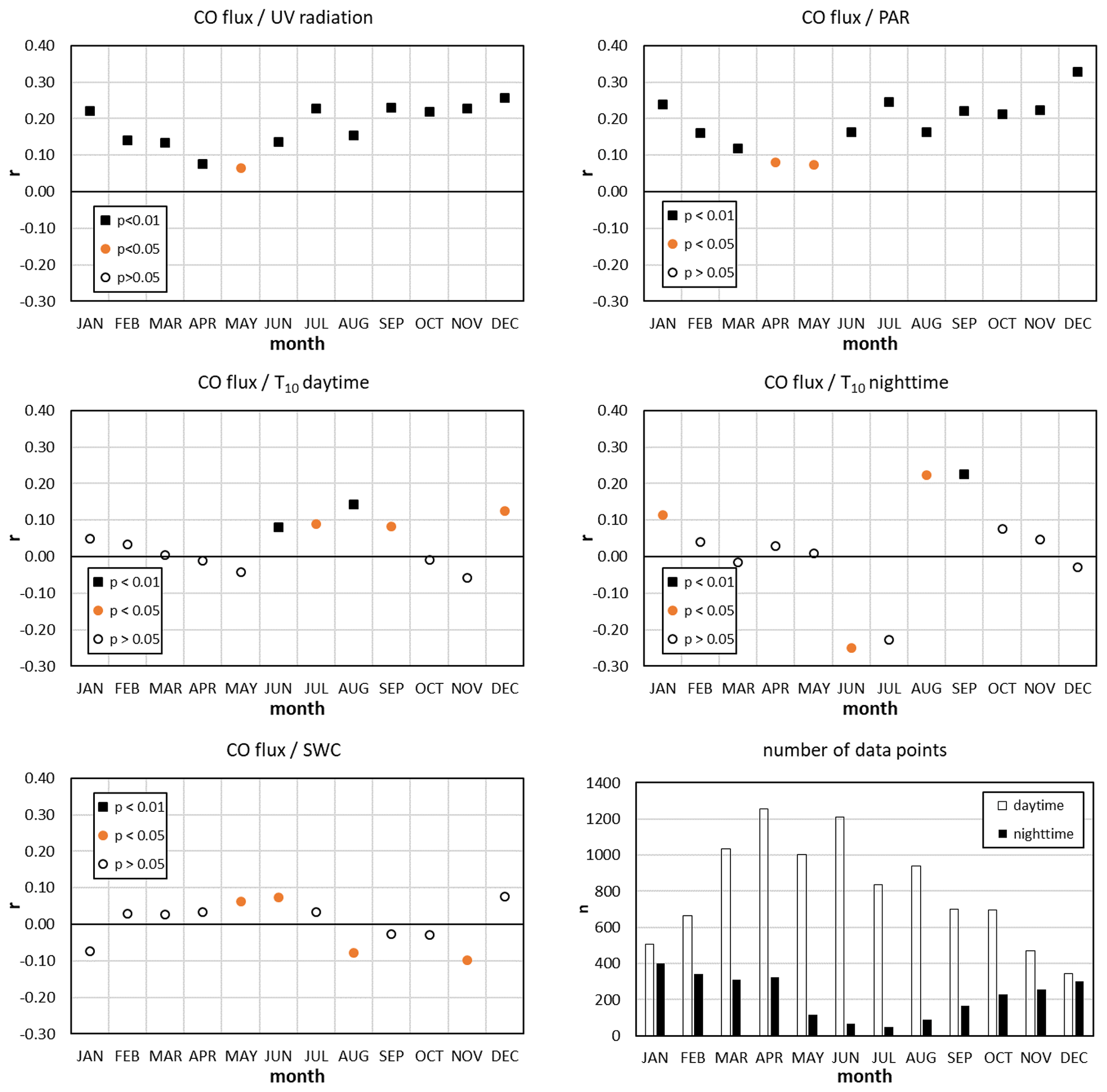
Figure 8 Monthly correlations (2015–2025) of CO fluxes with UV radiation, photosynthetically active radiation (PAR), air temperature at 10 m (T₁₀ – day and night), and soil water content, as well as the number of data points available for the correlation calculations. The different symbols indicate the confidence level of the correlation coefficients.

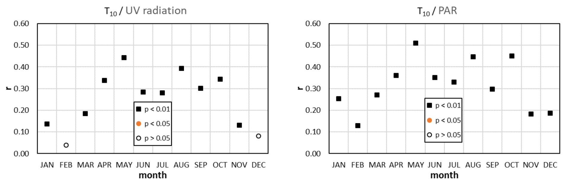
Figure 9 Correlations between air temperature and solar radiation. The wintertime low level of correlation is not a surprise. At this time of the year, clear sky is usually observed together with cold air mass intrusions.

Soil moisture or soil water content is occasionally also mentioned as one of the drivers of CO exchange (Laasonen et al., 2025). However, in our study, the correlation between CO flux and local soil water content (SWC) in the top 0–7 cm layer is not statistically significant (Fig. 8). This suggests that SWC may not be an important driver, at least with the given soil/vegetation characteristics. It should be emphasized, however, that we used data from the ERA5 database with a resolution of 0.25°×0.25° for the calculation, while there may be very significant variations in soil moisture content, soil types, and structure within an area of this size. Therefore, the fact that we do not observe a correlation between flux and soil moisture content in the present study does not mean that such a correlation cannot exist.

4 Discussion

4.1 Carbon monoxide emission from the populated areas

The fluxes originating from the populated grid cells show a remarkable seasonal variation: the winter values are an order of magnitude higher than the summer values (Fig. 5). Since traffic-related emissions may be similar throughout the year, and since there is no notable industrial activity in the region, the additional winter emissions can be attributed to residential heating in the villages with relatively high confidence. Although natural gas is available for residential heating, many households in this relatively poor, slowly depopulating region use biomass (wood, agricultural waste) or low-quality coal in technologically outdated, inefficient, poorly ventilated heating appliances. Unfortunately, illegal household waste burning is also rather common in such regions with poor socioeconomic conditions (Haszpra et al., 2022; Balogh et al., 2025). These circumstances can result in high CO emissions.

According to the EDGAR v8.1_AP database (Cripa et al., 2026) containing 0.1°×0.1° gridded CO emission data up to 2022, approximately 98 % of anthropogenic emissions from the EDGAR grid cell including the monitoring site origined from road transport (IPCC 2006 category: 1.A.3.b, IPCC, 2006) and residential (IPCC 2006 category: 1.A.4) emissions in 2015–2022. Transport emissions hardly change throughout the year. According to the database, the residential emissions in summer are only about 10 % of the transport emissions. Our measurement recorded 15.2 $\mathrm{nmol}{\mathrm{m}}^{-\mathrm{2}}{\mathrm{s}}^{-\mathrm{1}}$ CO emissions for May–September (non-heating season) on average, of which 13.7 $\mathrm{nmol}{\mathrm{m}}^{-\mathrm{2}}{\mathrm{s}}^{-\mathrm{1}}$ may be attributed to the transport sector (90 % of the total). The populated grid cells for which this value was calculated cover 12.8 % of the EDGAR grid cell (84.3 km²) including the tower. Considering the summer value to be valid for the entire year, the total CO emissions of transport origin are 131 Mg yr⁻¹ from the EDGAR grid cell. This value is twice as high as the EDGAR v8.1 average for the years 2015–2022 (60 Mg yr⁻¹).

The annual average flux over a populated grid cell is 48.1 $\mathrm{nmol}{\mathrm{m}}^{-\mathrm{2}}{\mathrm{s}}^{-\mathrm{1}}$ (see Fig. 5). Taking into account the total area of the populated grid cells within the EDGAR grid cell ($\mathrm{84.3}{\mathrm{km}}^{\mathrm{2}}\times \mathrm{0.128}=\mathrm{10.8}{\mathrm{km}}^{\mathrm{2}}$), and summing up the emissions for a year, we obtain that the total measured anthropogenic emissions expressed in mass of CO are around 460 Mg yr⁻¹, from which 330 Mg yr⁻¹ can be attributed to residential activity, primarily heating. Although we neglected small terms in the above estimation, including the few percentage shares of non-transport/non-residential emissions and the anthropogenic emissions recorded in the agricultural/forest areas, the EDGAR data for the residential sector (83 Mg yr⁻¹, averaged for 2015–2022) seems far too low. In addition, we cannot see the reasons for the 30 % reduction in emissions reported by EDGAR for the period from 2015 to 2022. Given the economic stagnation and deterioration between 2015 and 2022, including the impact of the COVID pandemic, we would expect an increase in the burning of biomass and other waste, and thus an increase in CO emissions, although this cannot be substantiated in the absence of surveys. Unfortunately, the small share of the populated grid cells in our monitoring area and the resulting limited amount of data prevent us from determining the actual emission trends.

4.2 Carbon monoxide exchange of the vegetation-dominated landscape

The dominant role of photodegradation in natural CO emission and the less intensive solar radiation during the winter months should result in less positive net CO exchange, even if the microbiological CO uptake must also be lower due to the lower temperature. However, the seasonal variation of CO exchange in the agricultural/forested areas shows a maximum in winter (Fig. 7). The elevated winter emissions over the vegetation-dominated areas are also reflected in Fig. 6. Murphy et al. (2023) also observed a winter increase in the CO fluxes over a grassland. Despite performing EC measurements on a 2.2 m-tall tower with a limited footprint, they identified the influence of distant anthropogenic sources. The area influencing our measurements performed at 82 m elevation can be about two orders of magnitude larger, and may cover different distant anthropogenic sources. This is true even when the “clean air” sector is carefully selected and constrained to footprints for which the contribution of the distant sources (outside of the 5 km radius of the tower) to the flux measured at the tower is less than 20 %. The wintertime emission in the populated grid cells can be two to three orders of magnitude larger than in the (quasi)natural grid cells. Even if the weighted footprint contribution from a distant grid cell is minor, the potentially huge emission from that cell may substantially influence the measured fluxes. This effect cannot be completely eliminated with our rather simple correction algorithm.

However, even with the unavoidable seasonally varying anthropogenic influence in mind, our measurements show that agricultural fields and forests are net sources of CO throughout the year. Our measurement results fall within the range of other measurements of −3– +14 $\mathrm{nmol}{\mathrm{m}}^{-\mathrm{2}}{\mathrm{s}}^{-\mathrm{1}}$ over grasslands and arable lands (van Asperen et al., 2015; Pihlatie et al., 2016; Cowan et al., 2018). Earlier longer-term EC measurements recorded diurnal CO flux variations similar to our measurements. Pihlatie et al. (2016) reported a distinct diurnal pattern with uptake at night and emission during the day. Their daytime maximum median emissions over the perennial reed canary grass reached 2.7 $\mathrm{nmol}{\mathrm{m}}^{-\mathrm{2}}{\mathrm{s}}^{-\mathrm{1}}$ around noon, while the nighttime values varied around −0.77 $\mathrm{nmol}{\mathrm{m}}^{-\mathrm{2}}{\mathrm{s}}^{-\mathrm{1}}$ throughout the measurement period. Cowan et al. (2018) also measured fluxes that showed a regular diurnal cycle peaking at noon (1–4 $\mathrm{nmol}{\mathrm{m}}^{-\mathrm{2}}{\mathrm{s}}^{-\mathrm{1}}$) and falling to around zero ($>-\mathrm{1}$ $\mathrm{nmol}{\mathrm{m}}^{-\mathrm{2}}{\mathrm{s}}^{-\mathrm{1}}$) at night. Laasonen (2021) recorded daytime net emission up to 3 $\mathrm{nmol}{\mathrm{m}}^{-\mathrm{2}}{\mathrm{s}}^{-\mathrm{1}}$ in forest, wetland, and cropland ecosystems in summer. These ecosystems showed zero flux or small uptake during nighttime. Murphy et al. (2023) observed a similar diurnal pattern, also in summer. During daytime, the measured fluxes were 1–5 $\mathrm{nmol}{\mathrm{m}}^{-\mathrm{2}}{\mathrm{s}}^{-\mathrm{1}}$, while the nighttime values were near zero or slightly negative ($>-\mathrm{2}$ $\mathrm{nmol}{\mathrm{m}}^{-\mathrm{2}}{\mathrm{s}}^{-\mathrm{1}}$). Recent measurements by Laasonen et al. (2025) over peatland also showed the characteristic daily cycle with a daytime maximum of 1.1 $\mathrm{nmol}{\mathrm{m}}^{-\mathrm{2}}{\mathrm{s}}^{-\mathrm{1}}$ and a nighttime minimum of −0.44 $\mathrm{nmol}{\mathrm{m}}^{-\mathrm{2}}{\mathrm{s}}^{-\mathrm{1}}$.

EC measurements at an elevation of 82 m would require the calculation of the storage term, i.e., the amount of CO accumulating below the measurement elevation in the cases of decoupling from the surface due to low-level temperature inversions (Haszpra et al., 2005). Ignoring the storage term can result in unrealistic flux values when the inversion layer breaks up and can also cause a slight bias during the formation of the nighttime inversion. Due to the lack of concentration profile measurements, we could not calculate the storage term. This could increase the uncertainty of the diurnal variation of the fluxes in the winter months during the hours when stable stratification forms or the inversion is breaking up. However, as there is no long-term accumulation or depletion of CO below the EC level, the storage flux is negligible already at the daily scale, and the missing storage term does not affect the total fluxes.

4.3 Drivers of the ecosystem carbon monoxide budget

Despite ongoing research, substantial uncertainty remains regarding the soil and vegetation processes that contribute to CO emission and uptake (King, 2000; Constant et al., 2008; Bruhn et al., 2013; Liu et al., 2018; Sun et al., 2018; Laasonen et al., 2025). This knowledge gap also hampers the development of process-based biogeochemical models of CO exchange (Liu et al., 2018). From the atmospheric point of view, the commonly studied drivers are solar radiation (see e.g. Bruhn et al., 2013; van Asperen et al., 2015; Pihlatie et al., 2016; Cowan et al., 2018; Murphy et al., 2023; Laasonen et al., 2025; and references therein), temperature (Constant et al., 2008; van Asperen et al., 2015; Murphy et al., 2023; van Asperen et al., 2024), and soil moisture (Cowan et al., 2018; Murphy et al., 2023; Laasonen et al., 2025). However, the results are uncertain and partly controversial, presumably due to the different climate and soil conditions, different vegetation types at the measurement sites, as well as the short measurement durations.

Most previous studies agree that photo- and/or thermal degradation of organic substances is/are the main driver(s) of the ecosystems' CO emissions. The key role of solar radiation (global radiation, UV or PAR spectra of the visible range) in CO emission has been confirmed already in the early studies on natural CO flux (see e.g. Seiler and Giehl, 1977; Tarr et al., 1995; Schade et al., 1999; Bruhn et al., 2013; Pihlatie et al., 2016; Murphy et al., 2023; Laasonen et al., 2025; and references therein). However, the importance of the role of thermal degradation is somewhat controversial. One of the reasons is that both emissions resulting from the abiotic thermal degradation and microbiological uptake are temperature-dependent (Whalen and Reeburgh, 2001). Some of the methods applied in the field (e.g. micrometeorological methods) measure the net surface-atmosphere exchange and cannot separate the emission and uptake processes. On the other hand, temperature is strongly correlated with solar insolation. According to the measurements of Laasonen et al. (2025), solar radiation is the primary driver of CO flux; the role of air temperature is limited. Murphy et al. (2023) and Cowan et al. (2018) found a variable relation between CO flux and temperature. On the contrary, the laboratory and field measurements of van Asperen et al. (2015) indicated a higher importance of thermal degradation than of photodegradation in CO flux.

Our measurements support the assumption that thermal decomposition either plays a minor role in CO emissions or is largely compensated by the microbiological uptake. The collinearity between temperature and solar radiation can lead to the incorrect identification of the causal relationships that may explain the controversy in the literature.

The role of SWC as a driver cannot be confirmed by our results. However, it should be noted that SWC may vary greatly within the footprint area due to the diversity of land use (presence of summer and winter crops with different phenophases, associated rooting depths, evapotranspiration rates, etc.). Therefore, the above conclusion should be treated with caution.

5 Conclusions

The evaluation of 10-year-long tall tower EC-based carbon monoxide flux measurements has revealed the advantages and challenges of such monitoring projects. The tall-tower EC measurements and their associated large flux footprints can provide information on heterogeneous, regionally characteristic landscapes that help the upscaling of the results. However, the high elevation causes gaps in the data series due to occasional decoupling from the surface. In principle, footprint modelling can separate the flux contribution from different land cover types. However, the emissions from populated areas are orders of magnitude larger than the CO exchange of natural or quasi-natural (agricultural fields, grasslands, forests) areas. Therefore, even distant anthropogenic sources can significantly influence measurements with footprints in areas covered almost exclusively by vegetation. This makes it difficult to study the dynamics of the CO exchange of the soil-vegetation system.

Despite the above-mentioned difficulties, our measurements support the theory that the primary driver of the CO exchange of the (quasi)natural ecosystems is solar radiation. The maximum emission can be observed in summer daytime (up to 2.66 $\mathrm{nmol}{\mathrm{m}}^{-\mathrm{2}}{\mathrm{s}}^{-\mathrm{1}}$, July hourly median at noon), while the nighttime exchange does not deviate statistically significantly from zero.

The measured emissions from the populated areas significantly exceed the emissions calculated using activity statistics. The discrepancies, ranging from a factor of 2 to 4, are far too large to be explained by uncertainties in the methodology or the input data alone and instead suggest that the real-world emission factors are substantially underestimated. It is hypothesized that the bottom-up method underestimates the fact that despite the supply of natural gas in this region, a significant proportion of the population heats their homes with technologically outdated heating appliances using wood, low-quality coal, agricultural or household waste for economic reasons. As the atmospheric impacts of CO depend on the amount of CO actually released into the air, it is of high importance to refine the emission factors applicable in real-life situations by field measurements. If the anthropogenic emission density recorded in the region of our measurement site were representative of the other rural regions in the country, the national total emissions reported to international organizations would need to be modified upward.