Simultaneous ground-based observations of a large quasi 26 d wave from three different measurement sites in northern mid-latitudes

We present simultaneous observations of a remarkable planetary wave event in mesospheric temperature observed by three different ground-based mid-latitude OH spectrometers at stations in Germany (Greifswald (54° N, 13° E), Wuppertal (51° N, 7° E), and Hohenpeißenberg (48° N, 11° E)) during boreal winter 2016/2017. Additionally, temperature profile observations with the satellite instruments SABER/TIMED and MLS/Aura are used for supporting information on the global distribution of the wave event.

The observed wave had a period of about 26 d and an amplitude of partly up to about 20 K. The satellite temperature observations confirmed that the wave signature exhibited all the characteristics of the well known Rossby (1,4) normal mode oscillation. To the best of our knowledge this is the first study reporting on such a strong Rossby (1,4) wave in the middle atmosphere of the Northern Hemisphere. The wave signature was also identified in atomic oxygen mixing ratios in the mesopause region and lower thermosphere observed with SABER illustrating the importance of such wave events not only for the temperature distribution but also for the temporal variation of trace-gas distributions.

1 Introduction

Planetary waves are large-scale phenomena that play a crucial role in the global circulation by transporting momentum from lower altitudes upward (e.g. Salby, 1984; Andrews et al., 1987; Volland, 1988). They are typically generated in the lower atmosphere and can propagate vertically, reaching also the mesosphere – lower thermosphere (MLT) region (50–110 km) under certain conditions (e.g. Holton, 1984; Laštovička, 1997; Smith, 2003; Sassi et al., 2012). Ground-based observations are known since decades to be particularly well suited for detecting such waves in the MLT region, employing a variety of techniques to monitor atmospheric parameters such as wind, temperature, and airglow, and they reveal periodicities that span from a few days to several weeks (e.g. Yoshida et al., 1999; Bittner et al., 2000; Espy et al., 2005; French et al., 2005; Stockwell et al., 2007; López-González et al., 2009; Day and Mitchell, 2010a, b; Takahashi et al., 2013; Zhao et al., 2019; Reisin, 2021). Within this broad spectrum, certain periodic fluctuations can be attributed to specific Rossby-wave modes, which, although modulated by the background wind field, emerge at relatively well-defined periods when typical background winds are present (e.g. Kasahara, 1980; Salby, 1981a, b). An observation of a large event with a period of about 28 d reported from an Antarctic station by Zhao et al. (2019) was interpreted as being associated with the Rossby-wave (1,4) mode, reinforcing the link between observed periodicities and underlying wave dynamics. Observations from the GRIPS instrument at the Wuppertal station have demonstrated the capability to also capture such wave events, and a previous analysis showed that a substantial proportion of detections fell within the 25 to 30 d period range (Kalicinsky et al., 2026). In the present study we extend this line of investigation by conducting a detailed analysis of one event within the same period band, incorporating additional ground-based stations and satellite observations to provide a more comprehensive view.

The paper first describes the instruments and datasets employed in Sect. 2, then presents the analysis of a specific winter 2016/17 event in Sect. 3, followed by a discussion of the results and their possible origin in Sect. 4, and finally offers a summary and conclusions.

2 Measurement data

2.1 OH*(3,1) rotational temperature observations

OH*(3,1) rotational temperatures in the mesopause region have been observed from the ground using GRIPS (GRound-based Infrared P-branch Spectrometer) instruments for several decades. The instruments measure three OH*(3,1) P-branch lines – P₁(2), P₁(3), and P₁(4) – in the near-infrared spectral range of 1.524 to 1.543 µm during night and cloud free conditions. The emission layer of excited hydroxyl molecules resides at approximately 87 km altitude with a thickness of about 9 km (Baker and Stair, 1988; Oberheide et al., 2006), but it can vary on different time scales (e.g. von Savigny, 2015; García-Comas et al., 2017). Rotational temperatures are then derived from the relative intensities of the three lines (see Bittner et al., 2000, and references therein) and these temperatures closely approximate kinetic temperatures in the mesopause region, particularly for the (3,1) vibrational band (Noll et al., 2015).

We use three different instruments located at the measurement sites Greifswald (54° N, 13° E), Wuppertal (51° N, 7° E), and Hohenpeißenberg (48° N, 11° E) in Germany (see Fig. 1). The measurements in Wuppertal started in the early 1980s, with continuous measurements since summer 1987. Two instruments conducted these measurements. GRIPS-II, a Czerny-Turner spectrometer with a liquid-nitrogen-cooled Ge detector (see Bittner et al., 2002, for a detailed instrument description), provided data until a detector failure in mid-2011. A new instrument was operated alongside GRIPS-II from early to mid-2011, yielding simultaneous measurements that revealed no significant differences between the systems. The new instrument, featuring similar optical properties but a thermoelectrically cooled InGaAs detector, faced technical issues causing data gaps in 2012 and 2013. After some final reconstructions the instrument called GRIPS-N has run reliably since early 2014 (Kalicinsky et al., 2016, 2024).

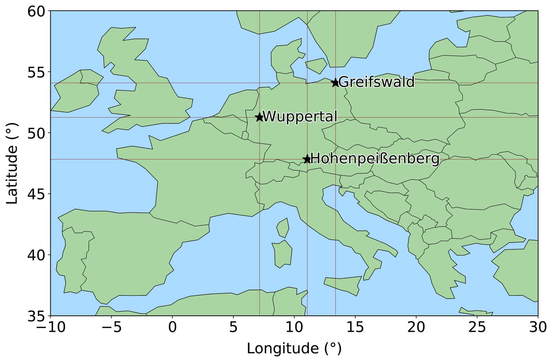
Figure 1 Geographical position of the three GRIPS instruments in Greifswald, Wuppertal, and Hohenpeißenberg.

The measurements in Hohenpeißenberg were done by GRIPS-I. This instrument is an Ebert–Fastie spectrometer with a liquid-nitrogen-cooled Ge detector (see Bittner et al., 2002, for a detailed instrument description). GRIPS-I started its operation in Hohenpeißenberg end of 2003 and the measurement time series ended in mid 2017 due to a final detector failure.

The observations in Greifswald are performed using an instrument largely identical in construction to the GRIPS 6 spectrometer described in Schmidt et al. (2013). The spectrometer in Greifswald has been operated continuously since 2015, with a single change in observation direction to the zenith in 2022. During the period relevant for the current analysis, the elevation angle was about 40°, so that the OH layer was observed roughly 100 km west of Greifswald.

The time resolution is best in Greifswald and worst in Hohenpeißenberg, because of the shorter and longer integration time (15 s vs. 270 s), respectively. Due to the longest integration time in Hohenpeißenberg, the possibility to encounter cloud influences within a single spectrum is enhanced. Thus, data gaps because of clouds are more frequently observed in Hohenpeißenberg than in Greifswald with Wuppertal (integration time 210 s) being in between.

The OH*(3,1) rotational temperatures exhibit a clear seasonal behaviour with lower temperatures in summer and higher temperatures in winter. This seasonal behaviour can be approximated via least-squares fitting of a model incorporating an annual, a semi-annual, and a ter-annual cycle:

$$\begin{array}{}\text{(1)}& T\left(t\right)=T_{\mathrm{0}}+\sum _{i=\mathrm{1}}^{\mathrm{3}}{A}_i\cdot \sin \left({\displaystyle \frac{\mathrm{2}\cdot \mathit{\pi }\cdot i}{\mathrm{365.25}}}(t+{\mathit{\varphi }}_i)\right),\end{array}$$

where t denotes the time in days, T₀ the annual mean temperature, and A_i, ϕ_i are amplitudes and phases of the sinusoids. Several previous studies have utilised this method and it proved to be a good concept (e.g. Bittner et al., 2000; Offermann et al., 2010; Perminov et al., 2014; Kalicinsky et al., 2016, 2024). The residual temperatures that will be analysed in this study are the difference of the measurements and the seasonal fit according to Eq. (1). As we analysed the winter 2016/2017 the fit was calculated from 1 July 2016 to 30 June 2017.

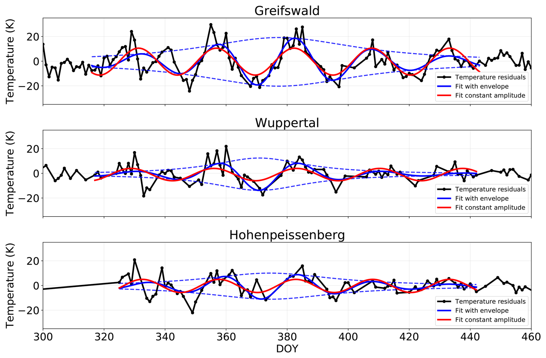
Figure 2 Temperature residuals of the OH*(3,1) rotational temperatures after subtraction of a seasonal fit at Greifswald, Wuppertal, and Hohenpeißenberg (top to bottom) during winter 2016/2017. The residuals are displayed as black curves together with fits to the data. First, a sinusoidal fit with amplitude modulation to the data from DOY 315 to 445 is shown as blue curve. The amplitude modulation follows a Lorentzian function and the envelope is shown as a blue dashed curve separately. Second, a sinusoidal fit with constant amplitude to the data in the same time interval is shown in red.

2.2 SABER observations

The Sounding of the Atmosphere using Broadband Emission Radiometry (SABER) instrument is an infrared limb radiometer positioned on the Thermosphere-Ionosphere-Mesosphere Energetics and Dynamics (TIMED) satellite. It started its scientific operation on 22 January 2002 and is active since. TIMED orbits the Earth in a non-sun-synchronous orbit (Russell et al., 1999; Esplin et al., 2023). For the current study, SABER Version 2.0 temperature and atomic oxygen profile measurements with a vertical resolution of about 2 km were used (Russell et al., 1999). Level 2A data was interpolated onto a regular 2 km geometric height grid and daily averaged in the region 48 to 57° N and 2° W to 28° E to compare it to temperature data sets over Greifswald (54° N, 13° E) and Wuppertal (51° N, 7° E). We restrict these direct comparisons to the two mentioned stations, as the number of data gaps is less compared to Hohenpeißenberg (see Sect. 2.1). Additionally, the SABER temperatures were also daily binned onto a global geographical grid with 5° latitude bins and 30° longitude bins.

2.3 MLS observations

Global temperature data was also used from the Earth Observing System Microwave Limb Sounder (MLS) that uses limb geometry to observe thermal emissions centered near 118, 190, 240 and 640 GHz as well as 2.5 THz. The instrument is located onboard the Aura satellite that performs a sun-synchronous orbit allowing latitude coverage between 82° N to 82° S. MLS started its scientific observations on 13 August 2004 (Waters et al., 2006). This study uses the Level 2 Version 5 temperature product that has an approximate bias with respect to SABER temperatures of +1 to −5 K between 1 and 0.1 hPa (ca. 50–65 km), 0 to −3 K between 0.1 and 0.01 hPa (65–80 km) and −10 at 0.001 hPa (ca. 95 km). The vertical resolution of MLS temperature profiles is 7–8 km at 1 to 0.1 hPa, 11 km at 0.01 hPa and 12 km between 0.0001 to 0.0002 hPa (ca. 105–110 km) (Livesey et al., 2022).

The temperature and geopotential height data used in this work were analysed according to the data documentation of Livesey et al. (2022). Only temperature profiles between a pressure range of 261 to 0.00046 hPa were used. Furthermore, the estimated precision of these profiles was required to be a positive number (to exclude data that is strongly impacted by the a priori information) and the status field (a quality metric provided for every profile containing a variety of flags) an even number. We only considered profiles with a data quality greater than 0.2 at 83 hPa and lower pressure levels, and a quality greater than 0.9 at 100 hPa or larger. The convergence field (describing how the fit of the radiances by the retrieval algorithm compares to the expected fit) needed to be less than 1.03 and we omitted profiles between 261 to 100 hPa with an ice water content larger than 0.005 g m⁻³ (at 215 hPa) to reduce the interference of clouds. The data was averaged for a global grid with 5° latitude bins and 30° longitude bins to investigate large scale wave patterns.

MLS geopotential height H is used to interpolate the MLS temperatures from a pressure grid to geometric altitudes z using the equation given by Guinn and Mosher (2015):

$$\begin{array}{}\text{(2)}& z={\displaystyle \frac{r\cdot H}{r-H}}\end{array}$$

Here, r is the mean Earth radius, set to 6 371 000 m.

3 Results

3.1 Ground-based observations of the wave event

The wave was simultaneously observed at three independent ground-based stations during the winter of 2016/2017. Pronounced temperature fluctuations are evident in the temperature residuals at all sites (see black curves in Fig. 2). The red curves in Fig. 2 additionally show fits of single sinusoids to the residual temperatures to illustrate the periodic behaviour. The determined amplitudes of the fits represent the mean amplitude of each fluctuation over the duration of the event. Within the interval of interest, the mean period is approximately 25 d at Hohenpeißenberg and Greifswald, and about 27 d at Wuppertal.

The corresponding moving Lomb–Scargle periodograms (LSP) (see Kalicinsky et al., 2020, 2024, for a description of the moving LSP) of the temperature residuals are presented in Fig. 3, where black contours mark regions of statistically significant spectral power. The significance is evaluated by use of the false alarm probability (FAP) that gives the probability that an observed flucutation is caused by chance, e.g. due to noise (see Kalicinsky et al., 2020, 2024, for more details). Obviously, the centre of the wave event at all three sites shows statistically significant results. Because of the larger amplitude at the station in Greifswald and the increased temporal coverage of the data due to weather conditions, the area of significant results is larger for Greifswald. Besides this systematic increase in amplitude of the flucuation with latitude, where the station farthest north shows the largest amplitude, also a distinct temporal amplitude modulation is evident.

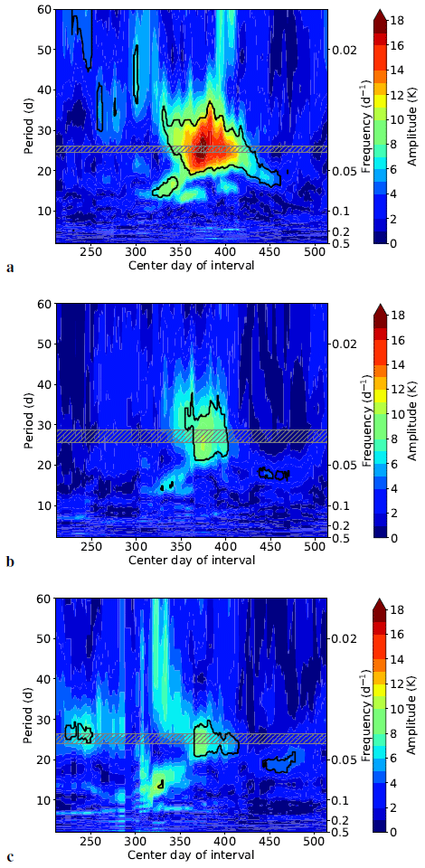
Figure 3 Moving-LSP results for (a) Greifswald, (b) Wuppertal, and (c) Hohenpeißenberg. The results have been obtained with a fixed window size of 60 d. The black lines mark the significant results and the gray hatched areas show the mean period ±2σ determined for the residual temperature time series between DOY 315 and 445 using the sinusoidal fit with fixed period (compare red curve in Fig. 2).

This temporal behaviour is most clearly demonstrated by fitting a sinusoidal function to the time series shown in Fig. 2, with the amplitude modulation parameterized by a Lorentzian-shaped envelope of the form:

$$\begin{array}{}\text{(3)}& {\displaystyle \frac{A_{max}}{\left(\mathrm{1}+{\left(\frac{(t-t_{\mathrm{0}})}{\mathit{\gamma }}\right)}^{\mathrm{2}}\right)}},\end{array}$$

where A_max is the maximum amplitude, t the time, t₀ the centre time, and γ the scale parameter.

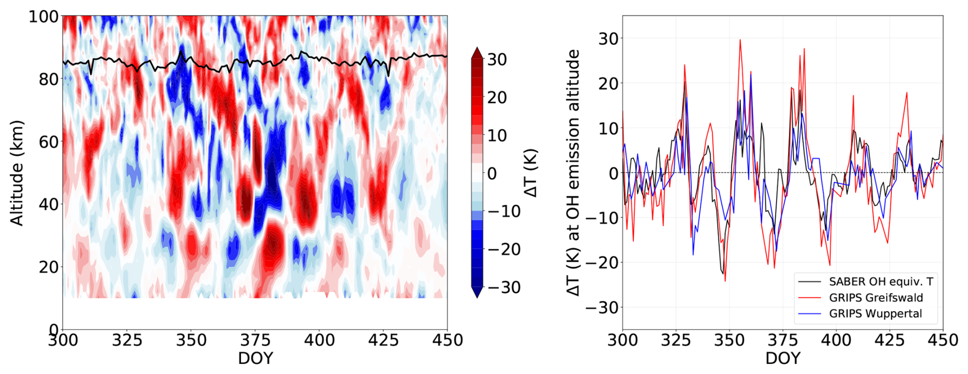
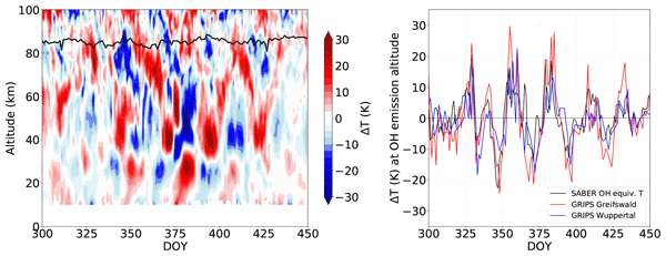
Figure 4 The left panel shows the SABER temperature anomalies for day and night time measurements in the latitude/longitude region 48–57° N and 2° W–28° E. The centroid altitude of the OH emission layer for the (3,1) band is displayed as a black curve. The right panel shows the time series of the temperature anomalies for the SABER OH equivalent temperatures as a black curve in comparison to the residual temperatures of the OH*(3,1) rotational temperatures observed from Greifswald (red curve) and Wuppertal (blue curve).

3.2 Satellite-based observations of the wave event

For comparison with the ground-based OH* rotational temperature measurements and to allow for a more comprehensive interpretation of the unusual dynamical situation during winter 2016/2017, which was the strongest wave event in this period range observed by our ground-based instruments in the last decade, we used mesospheric temperature observations derived from the MLS instrument as well as with SABER. The left panel of Fig. 4 shows the vertical and time dependence of temperature anomalies based on SABER temperature observations. Here the temperature anomalies were determined by subtracting a 41 d running mean from the SABER observations averaged over the Northern German longitude-latitude domain introduced above. The value of 41 is a subjective choice here, which is long enough for the mean to not follow the short periodic fluctuations but short enough to resemble the seasonal behaviour. Other values could also be used. Furthermore, a subtraction of a seasonal fit would be a possible way to obtain residuals, too, but it is omitted here as the exact description of such a fit describing the seasonal variations differs for each altitude level and depends also on the global region. Note that both daytime and nighttime SABER observations were used. In order to properly compare the temperature anomaly obtained from SABER observations with the temperature anomalies determined from the ground-based observations from Greifswald and Wuppertal, the corresponding SABER temperature profiles were averaged with weighting using the OH*(4–2) $/$ OH*(5–3) volume emission rate (VER) profiles also provided by SABER to obtain OH equivalent temperatures. Before this weighting the VER profiles were shifted downward by 0.75 km in order to consider that the OH centroid emission height increases by about 0.5 km per vibrational level (von Savigny et al., 2012a), because the ground-based instruments measure the OH*(3–1) band, while the SABER VER profiles correspond to the OH*(4–2) and OH*(5–3) bands. The shifted centroid OH emission altitude is shown as the black line in the left panel of Fig. 4. The right panel of Fig. 4 compares the temperature anomalies from the ground-based data sets with the corresponding SABER anomaly. Note here that the anomalies for the OH equivalent temperatures are determined in the same way as for the measured OH*(3,1) rotational temperatures by subtracting a seasonal fit (see Eq. 1). Apparently the overall agreement between the three anomalies is very good and all three data sets exhibit the remarkable quasi-periodic signature with an amplitude typically exceeding 10 K and partly even 20 K.

4 Discussion

A fluctuation with a period of 25–27 d lies within the range for which the maximum observation frequency for periodic fluctuations of OH*(3,1) rotational temperature was observed in more than 30 years of GRIPS measurements in Wuppertal (Kalicinsky et al., 2024). We hypothesize that a Rossby-wave (1,4) mode can account for a substantial portion of these observations and seek to demonstrate that the event presented in the current study indeed corresponds to such a mode. In the following paragraphs we investigate, whether the unusually large temperature perturbation during winter 2016/2017 discussed here exhibits all the characteristics of a Rossby wave (1,4) mode.

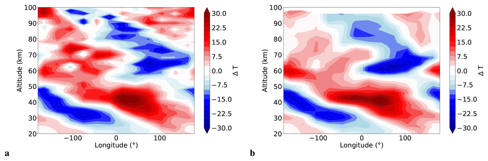
Figure 5 Vertical structure of the SABER (a) and MLS (b) temperature anomalies against the longitude in the latitude band 50–55° N on DOY 371.

First, a vertical cut through the temperature anomaly field along all longitudes in the latitude band 50–55° N on DOY 371, completing a global transect, is shown in Fig. 5a based on SABER observations and in Fig. 5b based on MLS observations. The figures reveal a clear zonal wave number 1 structure with antiphased behavior across different altitude regimes. Both satellite instruments concur here, although the MLS measurements exhibit reduced vertical resolution in the upper layers.

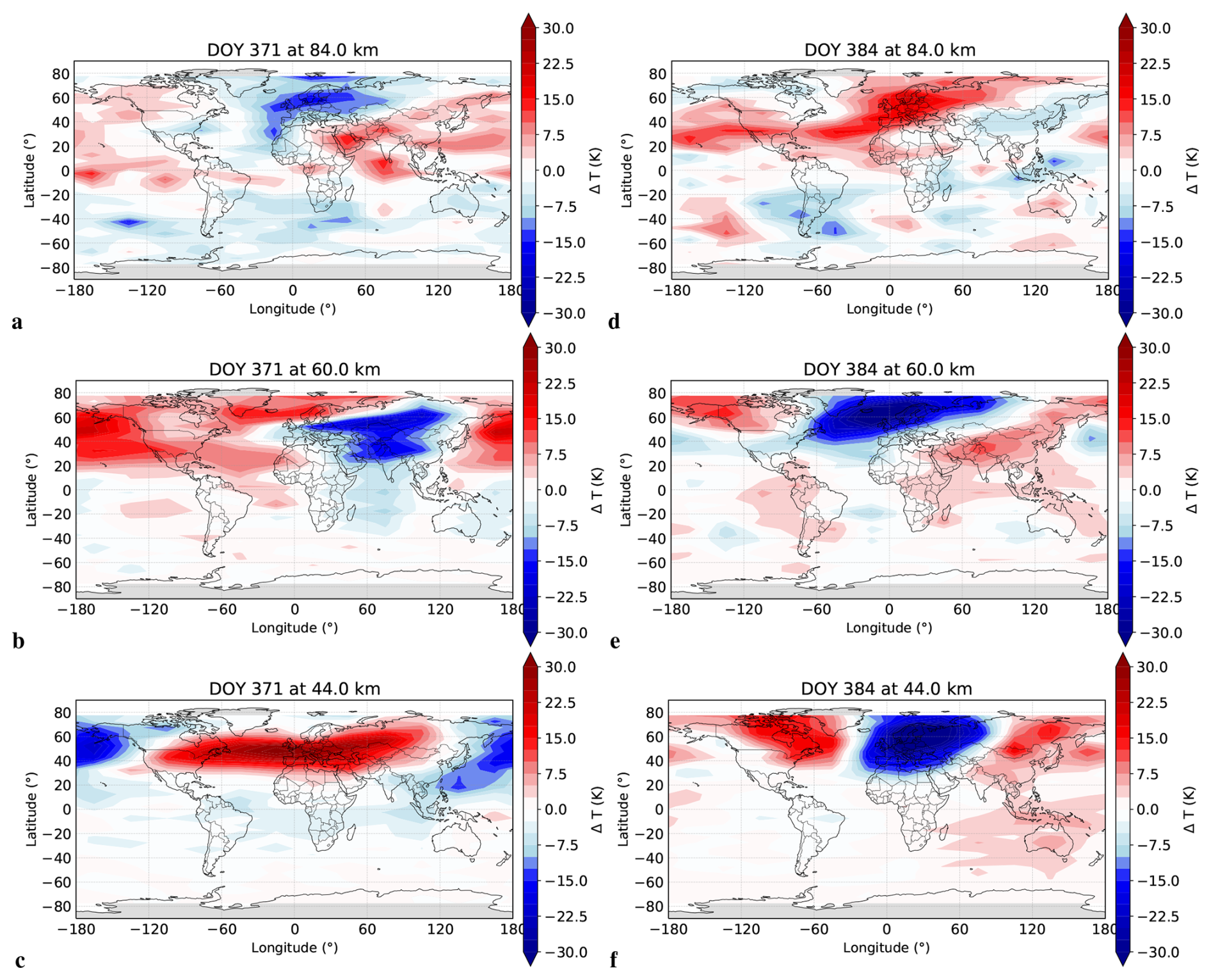
Figure 6 Horizontal maps of the MLS temperature anomalies at DOY 371 at the altitudes (a) 84 km, (b) 60 km, and (c) 44 km and the corresponding temperature anomalies at DOY 384 at the altitudes (d) 84 km, (e) 60 km, and (f) 44 km.

Second, horizontal maps of the MLS temperature anomalies at 84, 60, and 44 km on the same day display the same zonal wave number 1 pattern (see Fig. 6a–c). These maps are shown for MLS only as this instrument offers superior horizontal coverage but the temperature anomalies for SABER yield qualitatively identical results. Comparing DOY 371 with DOY 384 (see Fig. 6d–f), which is approximately half a period later, shows the temperature anomaly structures reversing colour (red to blue and vice versa) in many regions, indicating a periodicity of roughly 26 d.

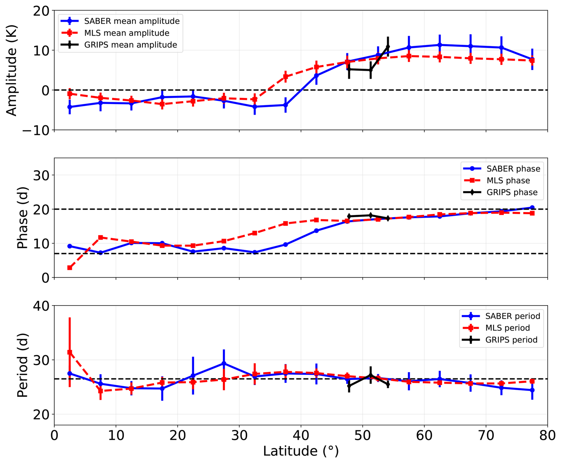
Figure 7 Latitude dependency of the mean amplitude, the phase, and the period of a sinusoidal fit to the data in the time interval DOY 315 to 445. The black curves show the results for the GRIPS OH*(3,1) rotational temperatures, the blue curves for the SABER temperature anomalies at 84 km in the longitude bin 0–30° E, and the red curves for the MLS temperature anomalies at the same altitude and longitude bin. The error bars mark the 2σ uncertainties.

Third, the meridional structure is less apparent in the horizontal maps but becomes discernible in parts of the 84 km height field, likely masked by other fluctuations. Consequently, we fitted sinusoids to the time series for all latitude boxes in the Northern Hemisphere in the longitude range 0–30°  E using both MLS and SABER temperature anomalies at 84 km to improve the determination of the meridional structure. The altitude and the geographical location were chosen according to the ground-based stations. The results for the periods, amplitudes, and phases are shown in Fig. 7. The mean fitted period is about 26.5 d. The sinusoid phases are expressed as the time lag in days of the first temperature maximum after a reference date, which is DOY 365. These phases cluster around 7 d and around 20 d, forming two groups roughly half a period apart, i.e. the oscillations are antiphased. The amplitudes of the fits are all taken as positive values in the first step and then assigned positive or negative according to the phases afterwards. In case of phases nearer to 20 d the amplitudes are assigned positive, whereas the amplitudes for phases nearer to 7 d are assigned negative. The latitudinal amplitude distribution exhibits two pronounced maxima of opposite sign in the Northern Hemisphere, consistent with a Rossby-wave (1,4) mode as proposed by Sassi et al. (2012) for the geopotential height (but the latitudinal distribution for the temperature is the same). The panels of Fig. 7 also show amplitude, phase and period of the wave event determined from the three ground-based OH*(3–1) temperature data sets used here. Apparently, the mean GRIPS amplitudes, periods, and phases agree well with the satellite observations. The latitudes of the GRIPS observations fall within the region of a steep amplitude increase with latitude in the satellite results, which can explain the observed differences at the ground-based measurement sites.

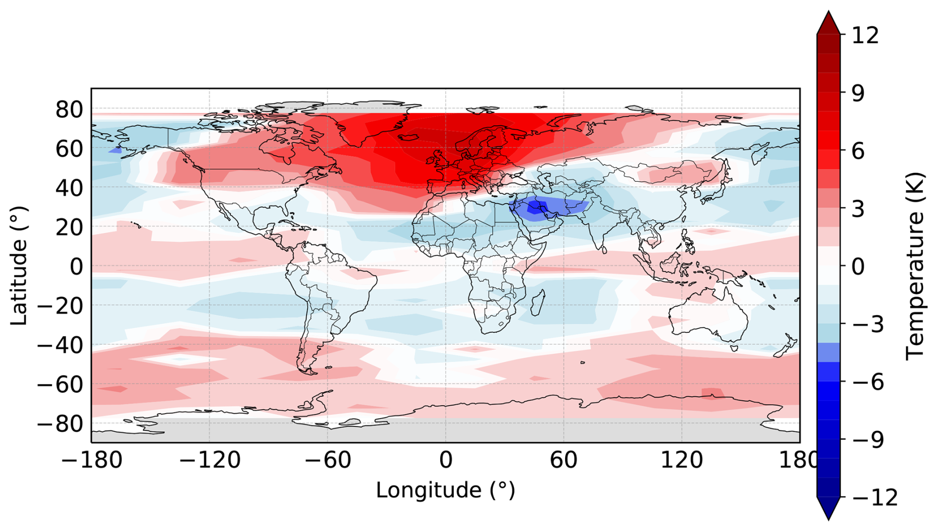
Figure 8 Global distribution of the amplitude of a sinusoidal fit to the MLS temperature anomalies in the time interval DOY 315 to 445. The positive and negative amplitudes are defined according to the phase. For details see text.

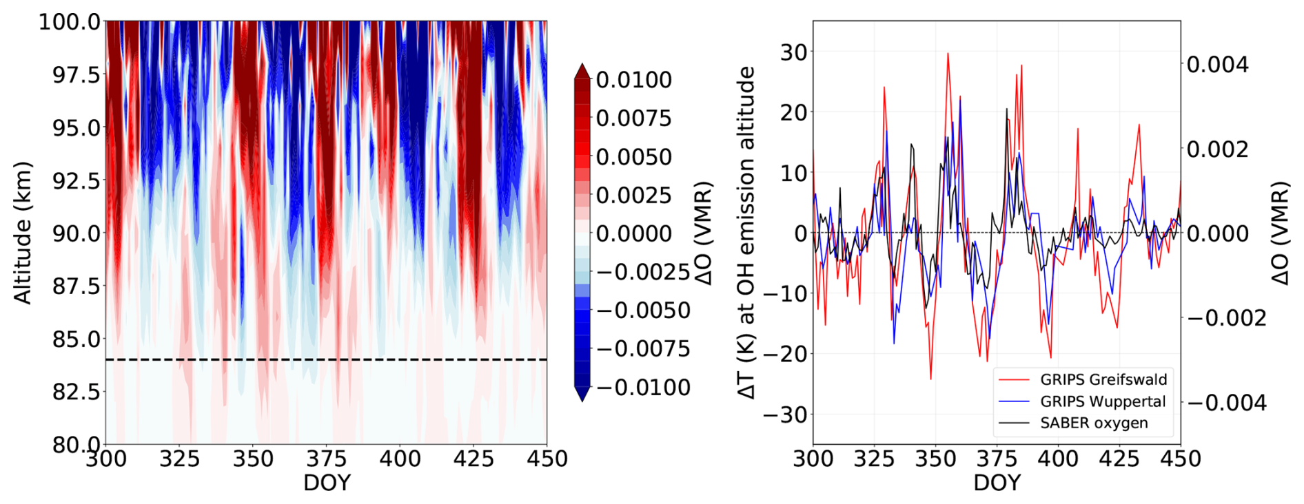
Figure 9 The left panel shows atomic oxygen anomalies derived from SABER observations in the latitude longitude region 48–57° N and 2° W–28° E. The right panel shows the anomalies at a height level of 84 km (corresponding to the dashed line in the left panel) in comparison to the OH*(3,1) rotational temperatures observed from Greifswald (red curve) and Wuppertal (blue curve).

Fourth, the same fitting procedure applied globally to the MLS temperature anomalies at 84 km reproduces the zonal wave number 1 structure in the Northern Hemisphere, with meridional amplitudes of opposite sign near the equator versus high latitudes (see Fig. 8). In the southern hemisphere, a complete sign reversal is evident at large western and eastern longitudes, though it is absent around 0° E. SABER anomalies show a comparable pattern when the sinusoid period is fixed at 26.5 d. Fits allowing a free period yield a noisier but qualitatively identical result, most likely due to data gaps at high northern and southern latitudes.

Collectively, these analyses substantiate that the observed 25–27 d temperature fluctuations are attributable to a Rossby-wave (1,4) mode.

The observed wave exhibits clear implications for other atmospheric constituents, as, e.g. atomic oxygen. Figure 9 illustrates the anomalies of atomic oxygen observed by SABER within the altitude range of 80–100 km in the left panel. The wave event is clearly detectable in atomic oxygen observations. Because the volume mixing ratios of atomic oxygen largely increase with altitude, the absolute effect of the wave intensifies at higher altitudes for the altitude range shown here. In the region of the centroid altitude of the OH layer the absolute effect is relatively small, but still visible. In the right panel of Fig. 9 a comparison between the oxygen anomalies at 84 km (approximately the centroid altitude of the OH layer during winter) and the OH*(3,1) rotational temperatures observed from Greifswald (red curve) and Wuppertal (blue curve) stations is presented. A pronounced correlation can be seen here: relatively higher rotational temperatures, which are indicative of downward motion of air masses and consequent adiabatic heating, coincide with relatively elevated oxygen values. This relationship can be interpreted as the result of downward transport of atomic oxygen from higher altitudes, where its volume mixing ratio is enhanced, whereas upward motions produce the opposite effect.

The results presented here possibly also have an effect on investigations of solar 27 d signatures in atmospheric parameters. Solar 27 d signatures have been identified in numerous middle atmospheric parameters including O₃ (Hood, 1986), OH (Shapiro et al., 2012), temperature (including OH* rotational temperature; von Savigny et al., 2012b) and noctilucent clouds (Robert et al., 2010). Usually, the solar 27 d signatures are identified either using cross-correlation analysis with a solar proxy variable (such as the solar F10.7 cm radio flux or the MgII index) or a superposed epoch analysis with a solar proxy time series as forcing time series. A Rossby wave (1,4) mode signature with amplitudes of 25 K and periods close to 27 d may interfere with the identification of solar 27 d signatures and lead to spurious identifications. The solar 27 d signature in stratospheric and mesospheric temperature has an amplitude of less than 1 K, i.e. much smaller than the possible amplitude of the Rossby wave (1,4) mode. With a superposed epoch analysis – for example – a large number of epochs is required to suppress a 25 K amplitude Rossby wave (1,4) mode signature with a similar period as the sun's rotation. We are not claiming that all previously identified solar 27 d signatures in middle atmospheric parameters are artifacts (see, e.g. Fig. 1 in von Savigny et al., 2012b or Fig. 3 in Stevens et al., 2026, where connections between temperature and the solar proxy are visible to the bare eye). However, future studies should investigate to what extent the detection and quantification of solar 27 d signatures in atmospheric parameters are affected by a Rossby wave (1,4) mode signature and how these different processes can be separated from each other.

5 Summary and conclusions

We presented observations of a remarkable planetary wave event in mesospheric temperature during boreal winter 2016/2017 with three different ground-based mid-latitude OH spectrometers and the satellite instruments SABER/TIMED and MLS/Aura. The wave signature had a period of about 26 days, an amplitude of up to about 20 K and covered almost four full cycles. Using the satellite temperature observations we confirmed that the wave signature exhibited all the characteristics of the well known Rossby (1,4) normal mode oscillation. Overall, we found very good agreement between the wave signature in temperatures retrieved from the ground-based and the satellite measurements. To the best of our knowledge this is the first study reporting on such a strong Rossby (1,4) wave in the middle atmosphere of the Northern Hemisphere. The wave signature was also identified in atomic oxygen mixing ratios in the mesopause region observed with SABER and can be expected to be present in other chemical species as well. Further research should clarify the impact of the Rossby (1,4) wave on investigations of solar 27 d signatures in middle atmospheric parameters.